Unsupervised Learning Layers for Video Analysis
Abstract
This paper presents two unsupervised learning layers (UL layers) for label-free video analysis: one for fully connected layers, and the other for convolutional ones. The proposed UL layers can play two roles: they can be the cost function layer for providing global training signal; meanwhile they can be added to any regular neural network layers for providing local training signals and combined with the training signals backpropagated from upper layers for extracting both slow and fast changing features at layers of different depths. Therefore, the UL layers can be used in either pure unsupervised or semi-supervised settings. Both a closed-form solution and an online learning algorithm for two UL layers are provided. Experiments with unlabeled synthetic and real-world videos demonstrated that the neural networks equipped with UL layers and trained with the proposed online learning algorithm can extract shape and motion information from video sequences of moving objects. The experiments demonstrated the potential applications of UL layers and online learning algorithm to head orientation estimation and moving object localization.
1 Introduction
Deep neural networks (DNNs) are powerful and flexible models that can extract hierarchical and discriminative features from large amounts of data. Despite their success in many supervised tasks such as image classification [16, 10], speech recognition [36] and machine translation [5], DNNs are data hungry which limits their applications in many domains where abundant annotated data are not available. This motivates us to explore almost infinite amount of unlabeled data for obtaining good representations that generalizes across tasks.
Learning from unlabeled data, often named as unsupervised learning, can be divided into four levels: learning from unlabeled images, from unlabeled videos, from virtual environment, or from the real environment directly. In this paper, we focus on unsupervised learning from label-free videos.
One of the main challenges of unsupervised learning is to derive good training signals. For supervised learning, we use the difference between the prediction from a DNN and the annotated ground truth as training signal. For unsupervised learning, there are two ways to obtain such signal: one is to design auxiliary tasks such as reconstructing the input image [12, 2, 17], predicting the next fewer frames given the first fewer frames in a video [31, 6, 20], reordering the shuffled video frames [23], generating fake images/videos in a generative adversarial network settings (GAN) [9], etc; another is to provide constraints [34, 11, 19, 32] that describe the desired structure of the output from a DNN. Our work belongs to the latter one.
Inspired by human visual system that can learn invariant representations and structures of objects from temporal experiences [7, 34], we design an objective function that constrains the output from a DNN to be temporally consistent meanwhile avoiding degenerated cases.
We evaluate our proposed algorithm in both synthetic and natural video settings. Experiments with end-to-end training on unlabeled-videos and applications to head orientation estimation and moving object localization demonstrated the effectiveness of the proposed algorithm.
The contributions of this paper are the following:
-
•
We design two unsupervised learning layers (UL layers) for label-free video analysis: one for fully connected layers, and the other for convolutional layers. The proposed UL layers can play two roles: they can be the cost function layer for providing global training signal; meanwhile they can be added to any regular neural network layers for providing local training signals and be combined with the training signals backpropagated from upper layers for extracting both slow and fast changing features at layers of different depths.
-
•
Both a closed-form solution and an online learning algorithm for the two proposed UL layers are provided.
-
•
The UL layers can be applied to any neural network architectures and can be used in either pure unsupervised or semi-supervised settings. We evaluated the proposed algorithm on both synthetic and real-world videos, and show that it has potential application to head orientation estimation, and moving object localization.
The rest of the paper is organized as follows. We briefly review related work in Section 2. The detailed description of the proposed methods is given in Section 3 followed by experimental results in Section 4 and conclusion in Section 5.
2 Related Work
Our work is closely related to representation learning, unsupervised learning and its application to label-free video analysis. Here, we briefly review some related work in these areas.
Representation Learning: Learning good data representations (or features) is one of the main goals for any machine learning algorithms – no matter whether it is a supervised or unsupervised one. For unsupervised learning, we want the learned representations of the data makes it easier to build classifiers or other predictors upon them. The question is how to evaluate the quality of learned representations. In [8], Goodfellow et al. proposed a number of empirical tests for directly measuring the degree to which learned representations are invariant to different transformations. In [11], Higgins et al. devised a protocol to quantify the degree of disentanglement learned by different models. In [1], Bengio et al. list some properties/attributes a good representation should possess, such as sparsity, distributed among multiple explanatory factors, hierarchical organization with more abstract and invariant concepts [14, 34] higher in the hierarchy, temporal and spatial coherence. The listed properties provide us guide to design appropriate objective functions for learning such representations.
Unsupervised Learning: Unsupervised learning of visual representations is a broad area with a rich history and a large volume of work – ranging from classical K-means clustering [21], dimensionality reduction [29, 13], sparse coding [24, 18], RBMs(Restricted Boltzmann Machines)[12], autoencoders [2, 17], single-layer analysis [4], to more recent work such as VAEs(Variational Auto-Encoders) [15], GANs(Generative Adversarial Networks) [9], pixelCNNs [25], and pixelRNNs [26]. The increase of computational capabilities [27] also makes large-scale deep unsupervised learning possible.
Our work is closely related to unsupervised learning from label-free video. Videos provide import temporal constraints for machine learning algorithms and they are abundant on websites. Most recent work employ video prediction as an auxiliary task for learning useful representations. The argument is that if the algorithm can predict the next fewer frames well, it has to learn some features related to objects’ shape, motion, etc. These algorithms usually predict next frames at pixel [31], interstate [33], object location [32] levels using language models [28], motion transformation [6], LSTM [31], GAN [22], or probabilistic models [35].
Unlike the above work that relies on auxiliary tasks for unsupervised learning, our work belongs to constraints-based unsupervised learning. We design an objective function that constrains the output from a DNN to be temporally consistent meanwhile avoiding degenerated cases. [32, 34, 3] are the most related work. In [32], the authors propose to employ laws of physics as constraints for supervising neural network training. For tracking an object in free fall, they constrain the outputs from the neural network which encodes the object’s height should form a parabola; while for tracking the position of a walking man, the outputs should satisfy the constant velocity constraint. Therefore, they have to design different loss functions for different types of object motion. In contrast, our objective function is more general and can be used to analyze videos of any smoothly moving objects. In [34], the authors propose a slow feature analysis algorithm for learning invariant or slowly varying features and demonstrate that the learned functions have a good match with complex cell properties. Similar to our closed-form solution method, their objective function also constrains the output should vary as slowly as possible but keep a unit variance. Like our work, they also proposed two neural network implementations of the algorithm. The difference is that we designed two unsupervised learning layers for implementing our online algorithms. The UL layers can be integrated into any neural networks seamlessly.
3 Methods
3.1 Problem Formulation
In our label-free learning setting, the training set is of training video sequences. Each sequence consists of image frames. The goal is to learn an internal representation of and a function such that
| (1) |
where the optimization is over a predefined class of functions . The first term in Eq. (1) enforces temporal consistency constraint, and the second term is used for avoiding degenerate case where .
3.2 Closed-form Solution
Consider the case where the dimensional mapping function can be any function for the temporal data.
Let the objective function be
| (2) |
Suppose the dynamics is a Markov chain on points , then Eq. (2) can be rewritten as
| (3) |
where is the stationary distribution of the Markov chain and is the stationary distribution of adjacent pairs.
Let be the Laplacian matrix defined as
| (4) |
Let be the diagonal matrix such that .
Eq. (2) has a closed-form solution for the internal representation :
| (5) |
where is the matrix whose column vectors are the generalized eigenvectors of and , which is equivalent to the normalized-cut solution [30], and is an arbitrary rotation matrix (i.e. ). See Appendix A.1 for the proof.
3.3 Online Learning Algorithm
Although the above closed-form solution is appealing, it is computationally expensive for long video sequences and is not practical for real world situations where frames are captured one at a time. Therefore, we derive an online learning algorithm that can be applied to a deep neural network (See Appendix A.2 for the derivation).
Let be the current output from the neural network, be the short-term moving average, and be the long-term moving average. Then and can be updated as follows:
| (6) | ||||
| (7) |
where .
And short-term covariance and long-term covariance can be updated as follows:
| (8) | ||||
| (9) |
The update rule for the parameters is:
| (10) |
where
| (11) |
3.4 Two unsupervised learning layers
We implemented the online learning algorithm with two unsupervised learning layers – one for fully connected layers and the other for convolutional layers. For the output from fully connected layers, the covariances are calculated with respect to the whole vector; while for the output from convolutional layers, the covariances are calculated with respect to each feature map channel.
These layers can be added to different deep learning models and at different layers for providing a way to directly improve feature representation in each layer in an unsupervised learning manner. The weight term in Eq. 3 is determined based on the distance between the unsupervised layer and the input layer. The closer it is to the input, the larger should be. This is because at lower level, the receptive field of a node is smaller and the corresponding input signal tends to change faster. Therefore, the proposed unsupervised learning layers can capture both fast and slow features at different depths of a DNN.
Unlike in regular DNN layers where all gradients are calculated at backward stages, in the unsupervised layers, the partial derivatives are calculated at forward stages and then combined with the gradient from the upper layers in the backward stage.
Algorithm 1 shows a summary of the algorithm.
In summary, the proposed UL layers can play two roles: they can be the cost function layer for providing global training signal; meanwhile they can be added to any regular neural network layers for providing local training signals and combined with the training signals backpropagated from upper layers for extracting features at different changing paces. Therefore, the UL layers can be used in either pure unsupervised or semi-supervised settings with a supervised cost function layer and several UL layers following the regular hidden layers.
4 Experiments
The proposed algorithm can be applied to any neural networks. We conducted the following experiments to evaluate the performance of the algorithm.
4.1 Synthetic sequence
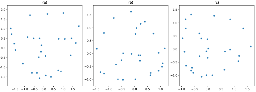
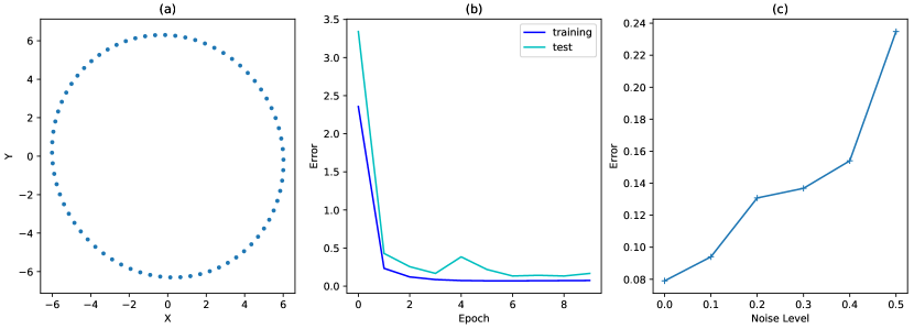
To evaluate the convergence speed and robustness of the proposed algorithm to noise, we generated synthetic video sequences consisting of a set of 28 randomly selected 2D points rotating around its centroid sampled at one frame per 5 degrees for training as shown in Fig. 1(a). The network consists of one fully connected layer followed by an unsupervised layer. The input size is 56 (=28 * 2) and the output 2. The hyperparameters are: learning rate=0.01, momentum=0.9, weight decay rate=0.1, . Fig. 1(b) and (c) visualize the two weight matrices learned in the fully connected layer which corresponds to the two major eigenvectors of the input sequence. Fig. 2(a) indicates that the output (each point corresponds to the output with respect to the input frame ) encodes the rotation angle of each frame in the sequence. This demonstrates that the neural network trained with our proposed algorithm can encode both input shape in the weights and motion in the output. We decoded the output using linear regression with respect to the sin function of rotation angles and calculated the total absolute errors between the output and the ground truth. Fig. 2(b) illustrates that the algorithm can converge within 10 epochs for both training and test set. To evaluate the noise sensitivity of the proposed algorithm, we tested the algorithm on five noise levels ranging from 0 to 50%. Fig. 2(c) demonstrates that the proposed algorithm exhibits a smooth degradation as the noise level is increased from 0 to 40%.
4.2 Head orientation estimation
To gain an understanding of the representations learned in the convolutional layers, we trained a neural network consisting of a regular convolutional and a fully connected layers, each followed by an unsupervised layer for predicting the head orientation from a video sequence (generated from Basel Face Model 111http://faces.cs.unibas.ch/bfm/?nav=1-0&id=basel_face_model. The hyperparameters are: learning rate=1e-5, L2 regularization weight decay rate = 0.01 and they are set the same for the rest of experiments.
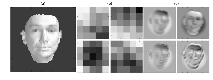
Fig. 3(a) shows one of the input image frame, Fig. 3(b) shows the learned four convolution kernels, and Fig. 3(c) shows the output from the convolutional layers which demonstrates that the learned representations captured the low-level features such as edges, corners and circles.
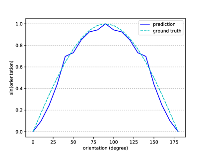
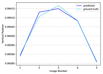
We also trained the network for video sequences (generated from QMUL Multiview Face Dataset222http://www.eecs.qmul.ac.uk/~sgg/QMUL_FaceDataset/ consisting heads doing pan rotation as shown in Fig. 4. and evaluated the accuracy of the output from the network which encodes the sin of head orientation as shown in Fig. 5.

4.3 Moving object localization
To gain an understanding of the performance of the proposed algorithm on DNN with real videos, we evaluated the algorithm on two datasets as the same as in [32]333https://github.com/Russell91/labelfree. The first task is to predict the location of a pillow tossed by a person as shown in Fig. 6. The dataset consists of 65 sequences of a pillow in flight, totaling 602 images. Images are resized to 56 x 56 pixels. For comparison purpose, we employ the same NN architecture as in [32] which consists of three convolutional layers followed by two fully connected layers and one unsupervised learning layer. Fig. 7(a) shows the qualitative results from our network after training on 32 sequences for 99 epochs. Since the author of [32] did not provide ground truth for this dataset, we did not perform quantitative performance evaluation for this dataset.


The second task is to predict the mask of a moving object in a video as shown in Fig. 8. The dataset consisted of color images of pixel size of (64, 64) with 10 sequences (261 frames) for training and 10 sequences (246 frames) for validation.
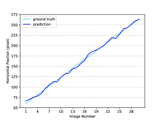
Fig. 8 shows the recovered masks and the centroids of the masks which locate the walking person correctly. Fig. 7(b) shows the comparison between the prediction and ground-truth. We estimate the correlation between our prediction and the ground truth which is 96.5% and is better than the one in [32] which is 95.4%.
5 Conclusion and future work
We presents two unsupervised learning layers (UL layers) for label-free video analysis: one for fully connected layers, and the other for convolutional layers. The proposed UL layers can play two roles: they can be the cost function layer for providing global training signal; meanwhile they can be added to any regular neural network layers for providing local training signals and combined with the training signals backpropagated from upper layers for extracting both slow and fast changing features at layers of different depths. Both a closed-form solution and an online learning algorithm implemented with two UL layers are provided. Experiments with training on both unlabeled synthetic and natural videos demonstrated the effectiveness of the proposed algorithm and its potential applications to head orientation estimation, moving object localization.
Several parts of the presented approach could be tuned and studied in more detail. The proposed unsupervised layers could be used in a semi-supervised setting. The temporal consistency constraint could be extended to spacial space. … We leave these questions for future research. We consider the present work as just a first step on the way to making an agent perform unsupervised learning in a real environment.
Acknowledgements
We thank our IDL members Haonan Yu, Zhuoyuan Chen, Haichao Zhang, Tianbing Xu, Yuanpeng Li, Peng Wang, Jianyu Wang, Xiaochen Lian and interns Qing Sun, Yaming Wang, Zhenheng Yang, Zihang Dai for their encouragement.
References
- [1] Y. Bengio, A. Courville, and P. Vincent. Representation learning: A review and new perspective. In TPAMI, 2013.
- [2] Y. Bengio, P. Lamblin, D. Popovici, and H. Larochelle. Greedy layer-wise training of deep networks. In NIPS, 2007.
- [3] P. Berkes and L. Wiskott. Slow feature analysis yields a rich repertoire of complex cell properties. In Journal of Vision, 2005.
- [4] A. Coates, A.Y. Ng, and H. Lee. An analysis of single-layer networks in unsupervised feature learning. In International conference on artificial intelligence and statistics, 2011.
- [5] Y. Wu et al. Google’s neural machine translation system: Bridging the gap between human and machine translation. In arXiv:1609.08144, 2016.
- [6] C. Finn, I. Goodfellow, and S. Levine. Unsupervised learning for phisical interaction through video prediction. In arXiv:1605.07157v2, 2016.
- [7] P. Foldiak. Learning invariance from transformation sequences. In Neural Computation, 1991.
- [8] I.J. Goodfellow, Q.V. Le, A.M. Saxe, H. Lee, and A.Y. Ng. Measuring invariances in deep networks. In NIPS, 2008.
- [9] I.J. Goodfellow, J. Pouget-Abadie, M. Mirza, B. Xu, D. Warde-Farley, S. Ozair, A.C. Courville, and Y. Bengio. Generative adversarial networks. In NIPS, 2014.
- [10] K. He, X. Zhang, S. Ren, and J. Sun. Deep residual learning for image recognition. In CVPR, 2016.
- [11] I. Higgins, L. Matthey, X. Glorot, A. Pal, B. Uria, C. Blundell, S. Mohamed, and A. Lerchner. Early visual concept learning with unsupervised deep learning. In arXiv:1606.05579v1, 2016.
- [12] G.E. Hinton, S. Osindero, and Y.W. Teh. A fast learning algorithm for deep belief nets. In Neural Computation, 2006.
- [13] G.E. Hinton and R.R. Salskhutdinov. Reducing the dimensionality of data with neural networks. In Science, 2006.
- [14] D.H. Hubel and T. Wiesel. Receptive fields, binocular interaction, and functional architecture in the cat’s visual cortex. In Journal of Physiology, 1962.
- [15] D.P. Kingma and M. Welling. Auto-encoding variational bayes. In ICLR, 2014.
- [16] A. Krizhevsky, I. Sutskever, and G.E. Hinton. Imagenet classification with deep convolutional neural networks. In NIPS, 2012.
- [17] Q.V. Le and et al. Building high-level features using large scale unsupervised learning. In ICML, 2012.
- [18] H. Lee, A. Battle, R. Raina, and A.Y. Ng. Efficient sparse coding algorithms. In NIPS, 2007.
- [19] K. Lin, J. Lu, C. Chen, and J. Zhou. Learning compact binary descriptors with unsupervised deep neural networs. In CVPR, 2016.
- [20] W. Lotter, G. Kreiman, and D. Cox. Deep predictive coding networks for video prediction and unsupervised learning. In arXiv:1605.08104v1, 2016.
- [21] J. MacQueen and et al. Some methods for classification and abalysis of multivariate observations. In the fifth Berkely symposium on mathematical statistics and probablity, 1967.
- [22] M. Mathieu, C. Couprie, and Y. LeCun. Deep multi-scale video prediction beyond mean square error. In arXiv:1511.05440v6, 2016.
- [23] I. Misra, C.L. Zitnick, and M. Hebert. Shuffle and learn: Upsupervised learning using temporal order verification. In ECCV, 2016.
- [24] B.A. Olshausen and D.J. Field. Emergence of simple-cell receptive field properties by learning a sparse code for natural images. In Nature, 1996.
- [25] A. Oord and et al. Conditional image generation with pixelcnn decoders. In arXiv:1606.05328, 2016.
- [26] A. Oord, N. Kalchbrenner, and K. Kavukcuoglu. Pixel recurrent neural networks. In ICML, 2016.
- [27] R. Raina, A. Madhavan, and A.Y. Ng. Large-scale deep unsupervised learning using graphics processors. In ICML, 2009.
- [28] M. Ranzato and et al. Video (language) modeling: a baseline for generative models of natural videos. In arXiv:1412.6604, 2014.
- [29] S. Roweis. Em algorithms for pca and sensible pca. In Techinical Report CNS-TR-97-02, 1997.
- [30] J. Shi and J. Malik. Normalized cuts and image segmentation. In TPAMI, 2000.
- [31] N. Srivastava, E. Mansimov, and R. Salakhutdinov. Unsupervised learning of video representation using lstms. In ICML, 2015.
- [32] R. Stewart and S. Ermon. Label-free supervision of neural networks with physics and domain knowledges. In AAAI, 2017.
- [33] C. Vondrick, H. Pirsiavash, and A. Torralba. Anticipating the future by watching unlabeled video. In arXiv:1504.08023, 2015.
- [34] L. Wiskott and T.J. Sejnowski. Slow feature analysis: Unsupervised learning of invariances. In Neural Computation, 2002.
- [35] T. Xue, J. Wu, K.L. Bouman, and W.T. Freeman. Visual dynamics: Probabilistic future frame synthesis via cross convolutional networks. In NIPS, 2016.
- [36] D. Yu and L. Deng. Automatic Speech Recognition. Springer, 2012.
Appendix A Appendix
A.1 Proof of the closed-form solution
Let be the vector , then Eq. (3) can be rewritten as
| (12) |
The minimum of is achieved when . That is
| (13) |
where .
This shows that is in a space spanned by generalized eigenvectors of and . Let the eigenvectors and corresponding eigenvalues be and , respectively. Then
| (14) |
where and .
And . Let , then Eq. (12) can be rewritten as
| (15) | ||||
| (16) | ||||
| (17) |
where , and .
is minimized when , and . Correspondingly,
| (18) |
Therefore in order to minimize , the eigenvalues should be the smallest ones except .
Let be a generalized eigenvector of and with eigenvalue . Note that vector whose all elements i are is also a generalized eigenvector of and with eigenvalue , therefore . Hence
| (19) |
which means that is also a generalized eigenvector of and and is equivalent to the normalized-cut solution [30].
In summary, the closed-form solution for Eq. 1 is:
| (20) |
where is an arbitrary rotation matrix (i.e. ).
A.2 Derivation of the online learning algorithm
We design the following cost function for the online learning algorithm:
| (21) |
where and denote the short-term and long-term covariances of the output from the neural network, respectively. The first term of Eq. 1 minimizes the entropy of short term distribution, while the second term maximizes the entropy of long term distribution. Therefore, the closer two input frames are, the closer their corresponding output representations would be; and the farther away the inputs are, the farther away their corresponding output representations should be.
Let be the short-term moving average, and be the long-term moving average. We have
| (22) | ||||
| (23) |
and we can derive
| (24) | ||||
| (25) | ||||
| (26) |
Similarly, we have
| (27) |
Hence,
| (28) | ||||
| (29) |
In summary,
| (30) | ||||
| (31) |
where and .