No snowball on habitable tidally locked planets
Abstract
The TRAPPIST-1, Proxima Centauri, and LHS 1140 systems are the most exciting prospects for future follow-up observations of potentially inhabited planets. All orbit nearby M-stars and are likely tidally locked in 1:1 spin-orbit states, which motivates the consideration of the effects that tidal locking might have on planetary habitability. On Earth, periods of global glaciation (snowballs) may have been essential for habitability and remote signs of life (biosignatures) because they are correlated with increases in the complexity of life and in the atmospheric oxygen concentration. In this paper we investigate the snowball bifurcation (sudden onset of global glaciation) on tidally locked planets using both an energy balance model and an intermediate-complexity global climate model. We show that tidally locked planets are unlikely to exhibit a snowball bifurcation as a direct result of the spatial pattern of insolation they receive. Instead they will smoothly transition from partial to complete ice coverage and back. A major implication of this work is that tidally locked planets with an active carbon cycle should not be found in a snowball state. Moreover, this work implies that tidally locked planets near the outer edge of the habitable zone with low CO2 outgassing fluxes will equilibrate with a small unglaciated substellar region rather than cycling between warm and snowball states. More work is needed to determine how the lack of a snowball bifurcation might affect the development of life on a tidally locked planet.
1 Introduction
M-dwarfs are the most common type of star in the galaxy, and in recent years there has been a large amount of work on whether tidally locked planets in the habitable zone of M-dwarf stars could host life (e.g., Joshi et al., 1997; Segura et al., 2005; Merlis & Schneider, 2010; Kite et al., 2011; Wordsworth et al., 2011; Pierrehumbert, 2011; Yang et al., 2013; Leconte et al., 2013; Menou, 2013; Hu & Yang, 2014; Yang et al., 2014; Hu & Yang, 2014; Kopparapu et al., 2016; Turbet et al., 2016; Ribas et al., 2016; Barnes et al., 2016; Meadows et al., 2016; Wolf, 2017; Bolmont et al., 2017). This topic is particularly timely given the recent discoveries of likely terrestrial planets in the habitable zones of three M-dwarfs within 40 light years of Earth (TRAPPIST-1e, Proxima Centauri b, and LHS 1140b, Anglada-Escudé et al., 2016; Gillon et al., 2017; Dittmann et al., 2017). One issue that influences planetary habitability is the occurrence of global glaciations, which are called snowball Earth events in Earth history (Kirschvink, 1992; Hoffman et al., 1998). Snowball Earth events are an acute stressor on life, but may actually increase the complexity of life through evolutionary pressure (Kirschvink, 1992; Hoffman et al., 1998) and by increasing the atmospheric oxygen concentration (Hoffman & Schrag, 2002; Laakso & Schrag, 2014, 2017). Oxygen itself is suggestive of life on a planet and complex life can emit various gases or other signals that might act as biosignatures to remote astronomers. Moreover, planets in the habitable zone with low levels of CO2 outgassing may experience limit cycles between habitable and snowball climate states (Kadoya & Tajika, 2014; Menou, 2015; Haqq-Misra et al., 2016; Batalha et al., 2016; Abbot, 2016; Paradise & Menou, 2017). It is therefore important to understand the transitions into and out of snowball events for tidally locked planets.
The difference in the top-of-atmosphere albedo between regions covered by ice or snow on the one hand and ocean or land on the other (henceforth simply the “ice/ocean albedo contrast”) creates a basic nonlinearity in the climate system (Budyko, 1969; Sellers, 1969). Both an ice-covered (snowball) and a mostly ice-free state like the modern climate can exist, even for the same external forcing (CO2, stellar flux, etc.). If the stellar flux is decreased in a climate model of modern Earth, eventually the replacement of surface water with highly-reflective ice (the ice-albedo feedback) overwhelms stabilizing feedbacks in the system (Roe & Baker, 2010). At this point the modern climate state ceases to exist and the climate plunges into a snowball state (Budyko, 1969; Sellers, 1969). This is an example of a saddle-node bifurcation (Strogatz, 1994), and we will call it the “snowball bifurcation” in this paper. The forcing parameter, such as stellar flux, must be increased beyond its value at the snowball bifurcation in order to deglaciate the snowball planet, which is a phenomenon called hysteresis. For a range of stellar fluxes both the warm and snowball states are possible, so the system is bistable.
When considering whether extrasolar planets orbiting stars different from the Sun might exhibit a snowball bifurcation, one important factor is that ice and snow absorb much better in the near infrared than in the visible (Joshi & Haberle, 2012; Shields et al., 2013). This means that the difference in albedo between ice and water will be smaller for an M-dwarf spectrum than for the Sun, which would decrease the range of insolation bistability associated with the snowball bifurcation (Shields et al., 2014). Another important aspect of temperate planets orbiting M-dwarf stars is that they are likely to be tidally influenced, and even tidally locked in 1:1 spin-orbit states (Kasting et al., 1993). Lucarini et al. (2013) performed simulations using PlaSim, an intermediate-complexity global climate model (GCM), for various planetary rotation rates, and found no snowball bifurcation as they varied the stellar flux for a tidally locked planet. However, they did not decrease the stellar flux enough to cause global glaciation (Boschi, R., personal communication, March 31, 2017), so we cannot rule out a snowball bifurcation based on these simulations. Hu & Yang (2014) performed simulations where they varied the stellar flux received by a tidally locked planet orbiting an M-dwarf in an atmospheric GCM (CAM3) coupled to either a mixed layer ocean or a dynamical ocean. They found a smooth transition from a partially to completely ice covered planet in both cases. This suggests the lack of a snowball bifurcation for tidally locked planets, although they did not show whether there was hysteresis in that paper.
In this paper we show that tidally locked planets are not required to have a snowball bifurcation, and in fact are unlikely to have one for realistic parameter assumptions. We show that a primary cause of this behavior is the steady increase in insolation as the substellar point is approached, which contrasts with the Earth-like case where the derivative of insolation with respect to latitude goes to zero as the equator is approached. An additional important factor is that the top-of-atmosphere ice/ocean albedo contrast is small for tidally locked planets because of strong cloud cover over open ocean on the day side. That said, it is possible for tidally locked planets to have a snowball bifurcation if they have very strong heat transport away from the substellar point or weaker day-side clouds. These conclusions are based on simulations using both an energy balance model (EBM, section 2) and PlaSim, an intermediate-complexity global climate model (GCM, section 3). We also discuss avenues for further pursuing work in this area in section 4 and conclude in section 5.
2 Energy Balance Model
2.1 Earth-like Planet
Here we will solve the Budyko-Sellers energy balance model (Budyko, 1969; Sellers, 1969) for an Earth-like, rapidly rotating planet. For more information see Abbot et al. (2011) and Roe & Baker (2010). This type of modeling is useful because it allows analytical solutions with clear interpretations. An EBM, however, should only be used to gain qualitative understanding of the climate system, rather than to make quantitative predictions.
Due to rapid rotation and a strong Coriolis force, we will assume that the planet is zonally (East-West) symmetric, as Earth approximately is. We will also assume that the planet is symmetric to reflection across the equator, so we only need to solve for one hemisphere. At steady-state, energy balance is given by
| (1) |
where is the solar constant, describes the meridional distribution of incoming solar radiation, is the surface temperature, is a linearization of the outgoing longwave radiation flux as a function of surface temperature, is a simple parameterization of the meridional redistribution of heat by the atmosphere and ocean, is a constant with the same units as , is the sine of the latitude with . is the albedo, with the form
| (2) |
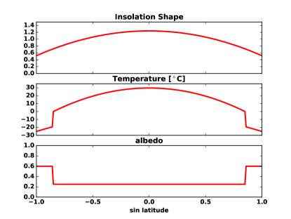
where is a low albedo representing open ocean regions, is a high albedo representing ice-covered regions, , and is the annual-mean surface temperature at which ice forms. We will use the insolation from North (1975), which we plot in Figure 1. The values assumed for the parameters are chosen for illustrative purposes.
We can solve the model to find the following relation for as a function of , the sine of the ice latitude,
| (3) |
where , the global mean albedo, is defined by
| (4) |
Eq. (3) represents the solution to the model containing both stable and unstable solutions (see Abbot et al. (2011) and Roe & Baker (2010) for a discussion of how to figure out which is which) and bifurcations when they join together (Figure 2). If we pick a particular value of Q, we can also plot the temperature as a function of latitude (Figure 1).
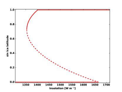
The snowball bifurcation in the Budyko-Sellers model corresponds to the ice latitude, , where =0. This condition can be written as
| (5) |
or simplifying
| (6) |
Physically, we can understand the snowball bifurcation as a competition between solar forcing and heat transport (Roe & Baker, 2010; Rose, 2015). Both the insolation (warming) and the divergence of the heat flux (cooling) increase as the equator is approached. If the ice latitude is such that when it is perturbed toward the equator the increase in absorbed insolation causes more warming than the increase in heat flux divergence causes cooling, then this ice latitude will be stable. If the opposite is true, then the ice latitude cannot be stable and a snowball bifurcation occurs. In the Earth-like configuration the derivative of insolation with latitude goes to zero at the equator. As long as (there is some poleward heat transport) and (there is some ice/ocean albedo contrast) this means that there will always be a point where the increase in the divergence of the heat flux exceeds the increase in insolation. A snowball bifurcation will occur at this point.
2.2 Tidally locked planet
We can easily modify the Budyko-Sellers model for the tidally locked configuration. We will use a coordinate system where the tidally locked latitude, , is the angle from the substellar point. The axis of symmetry here is from the substellar to the antistellar point. A tidally locked latitude of =0∘ corresponds to the substellar point, a latitude of =90∘ corresponds to the terminator, and a latitude of =180∘ corresponds to the antistellar point (Koll & Abbot, 2015, 2016). The insolation, , can be written
| (7) |
where is the solar zenith angle. First note that on the day side the solar zenith angle is equal to the tidally locked latitude as we have defined it (). We can therefore define the insolation shape function for use in Equation 1 as
| (8) |
where we are now using the variable , which is different from the Earth-like case. The tidally locked insolation profile is plotted in Figure 3.
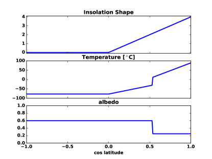
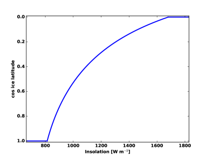
We can now apply the Budyko-Sellers model to this insolation profile. We calculate the global mean albedo by integrating over both the day and night sides as follows
| (9) |
Using Equation (3), the solution to the tidally locked Budyko-Sellers model is plotted in Figure 4. The first thing to note about the tidally locked solution is that for this set of parameters there is no snowball bifurcation. The reason is that the insolation keeps increasing strongly as the substellar point is approached (=1). This means the heat export has to be very strong for it to overwhelm the warming from increased insolation as the substellar point is approached. If we plug Eq. (8) into Eq. (6) we find that the ice latitude at which a snowball bifurcation occurs in the tidally locked model is
| (10) |
From Eq. (10) we can tell that for many parameter choices , so there is no snowball bifurcation. This is an important distinction from our condition for the snowball bifurcation in the Earth-like case (Eq. 6), which always yields a snowball bifurcation as long as and . We can set to solve for the critical value of , , that allows for a bifurcation
| (11) |
The tidally locked model will exhibit a snowball bifurcation for .
Eq. (11) has two important implications. First, it shows that if a tidally locked planet is efficient enough at moving heat from warm to cold regions ( is large enough), it is possible for a tidally locked planet to have a snowball bifurcation. This is important because one might assume that the same planet would have a higher value of if it were tidally locked because the strong heating and cooling anomalies on the day and night sides should force strong heat transport, and because the planetary rotation rate may be lower. Second, it shows that if the top-of-atmosphere ice/ocean albedo contrast is smaller, a planet is less likely to experience a snowball bifurcation ( increases). This is important because tidally locked terrestrial planets should have massive cloud decks on their day sides (Yang et al., 2013; Way et al., 2015; Kopparapu et al., 2016; Salameh et al., 2017). This should tend to increase the top-of-atmosphere albedo over open ocean regions, making the effective albedo contrast between ocean and ice/snow smaller. Moreover, planets orbiting M-stars should have smaller ice/snow albedos as a result of their stellar spectrum (Joshi & Haberle, 2012; Shields et al., 2013, 2014).
We can summarize the EBM results in the following way. As long as (the planet has an atmosphere) and (as it should generally be), an Earth-like planet will exhibit a snowball bifurcation. In contrast, the sharp increase in the insolation as the substellar point is approached means that a tidally locked planet will not have a snowball bifurcation for many parameter choices. Whether a tidally locked planet actually does exhibit a snowball bifurcation depends on planetary heat transport, ice/snow albedo, and cloud behavior.
3 Planet Simulator
3.1 Model
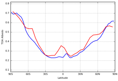
We use PlaSim (Fraedrich et al., 2005), an intermediate-complexity 3D global climate model (GCM), to explore the possibility of bifurcations and bistability for a tidally locked Earth-like planet. PlaSim solves the primitive equations for atmospheric dynamics and has schemes to calculate radiative transfer, convection and clouds, thermodynamic sea ice, and land-atmosphere interactions. One particular aspect of the sea ice scheme that will be relevant in later discussion is that it assumes a gridbox is either completely covered with sea ice or completely ice-free, so that partial sea ice coverage of a grid box is not allowed. We run the model at T21 horizontal resolution () with 10 vertical levels. We use modern Earth’s continental configuration and set the CO2 to 360 ppm. We use a 50 m slab ocean with zero imposed ocean heat transport. For the Earth configuration simulations we use modern Earth’s orbital configuration and rotation rate. For the tidally locked configuration simulations we set the orbital period (and rotation rate) to 10 Earth days and the eccentricity to zero. We set the obliquity to zero as is appropriate for planets in the habitable zone of M-dwarfs (Heller et al. 2011). We fix the time of day to a constant value in the shortwave radiation scheme. In order to isolate the effects of changes in orbital and rotational configuration, we use the Sun’s spectrum for all simulations, including the tidally locked ones. We accidentally used different versions of PlaSim’s modern Earth land-sea mask for the Earth and tidally locked configurations. Slight differences in the continental areas can be seen in Figure 6. We do not expect these slight differences to affect our conclusions. Given the importance of albedo for this paper, we tested PlaSim’s top-of-atmosphere albedo in the Earth configuration against modern Earth observations and found a good match (Figure 5).
Our methodology for exploring possible bifurcations, bistability, and hysteresis in PlaSim is as follows. For both the tidally locked and Earth configuration we perform a simulation at a high value of stellar flux that leads to a climate with no sea ice and a simulation at a low value of stellar flux that leads to a climate with an ocean that is 100% ice-covered. At various intermediate values of stellar flux we then start simulations from the equilibrated state of either the ice-free climate (henceforth Warm Start) or the ice-covered climate (henceforth Cold Start). We run all simulations until they reach top-of-atmosphere and surface energy balance, for a minimum of 50 years. We then average all displayed variables over the final 5 years of the simulations. If the equilibrated climates that result from Warm Start and Cold Start differ, then there is hysteresis. In the Earth configuration we will find hysteresis that is due to the snowball bifurcation and is associated with bistability. In the tidally locked configuration we will find a small amount of hysteresis that is an artifact of the sea ice scheme and is not related to the snowball bifurcation (Appendix A).
3.2 Results
3.2.1 Example equilibrated climates
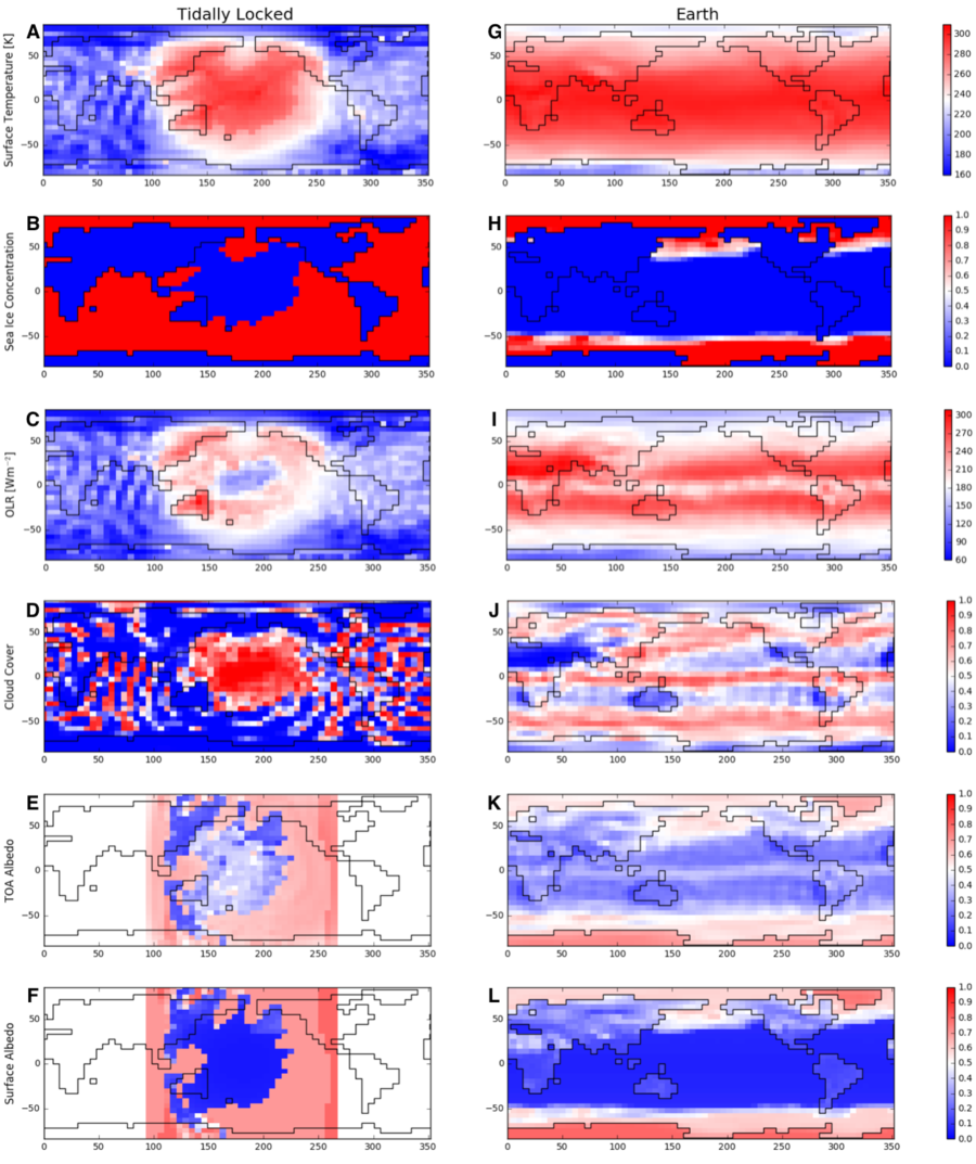
We first present maps of important model output for equilibrated annual mean climates of the tidally locked and Earth configurations (Figure 6). We used a stellar flux of 1367 W m-2, roughly modern Earth’s value, for the Earth simulation and initialize it from Warm Start conditions. We obtained a climate broadly similar to modern Earth’s, which confirms that the low resolution and approximations made by the PlaSim model are acceptable for this study. The features of PlaSim’s surface temperature simulation are remarkably similar to modern Earth given that it is an intermediate complexity GCM (Figure 6A). Sea ice is slightly more extensive than on modern Earth (Figure 6B), which may result from our neglect of ocean heat transport (Winton, 2003; Langen & Alexeev, 2004; Bitz et al., 2005; Rose, 2015). We should also note that partial sea ice coverage is possible in this plot because it is an annual mean. The cloud pattern (Figure 6D) shows the Inter-Tropical Convergence zone near the equator and the mid-latitude storm tracks, reflecting a reasonable simulation of atmospheric dynamics and clouds. The other variables are mostly determined by surface temperature, sea ice, and clouds, and they therefore approximate modern Earth well.
For the tidally locked reference simulation, we used a stellar flux of 1100 W m-2. The substellar surface temperature at this stellar flux is similar to the equatorial surface temperature on modern Earth, but the surface temperature is lower in some areas of the night side than at any point on modern Earth (Figure 6G). As a result, the ocean is covered in sea ice except for the region near the substellar point (Figure 6H). This is sometimes referred to as an “Eyeball” climate (Pierrehumbert, 2011). As expected for a tidally locked planet (Yang et al., 2013; Way et al., 2015; Kopparapu et al., 2016; Salameh et al., 2017) the open ocean region near the substellar point is mostly covered with clouds (Figure 6J). These clouds reflect stellar radiation and raise the top-of-atmosphere albedo (Figure 6K), so that the top-of-atmosphere albedo contrast between the sea-ice-free and sea-ice-covered regions is smaller in the tidally locked configuration than in the Earth configuration even though we use the same stellar spectrum for both configurations.
3.2.2 No tidally locked snowball bifurcation
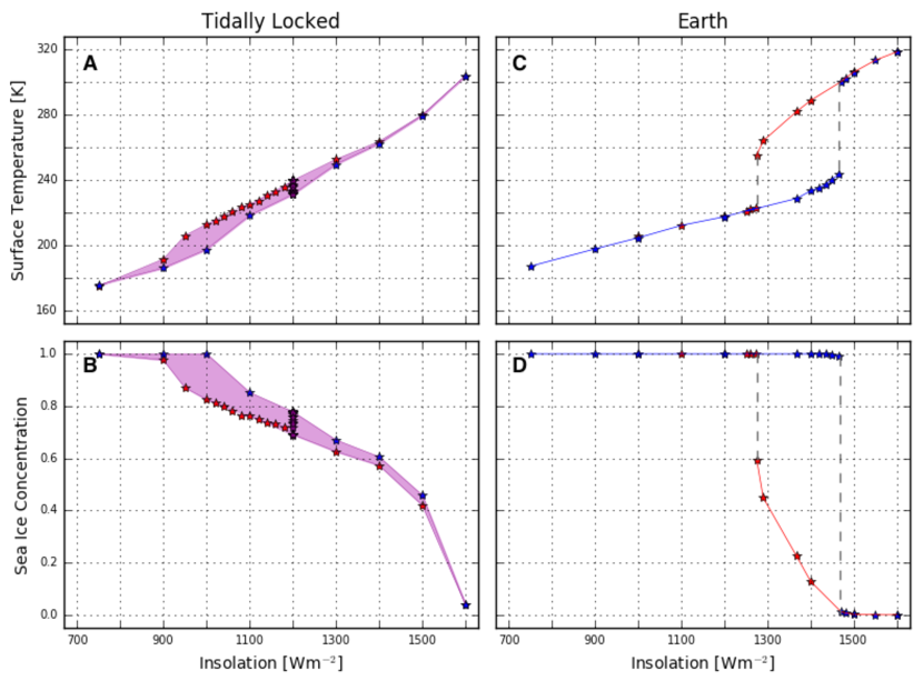
First we reproduce the well-known result that a snowball bifurcation exists for modern Earth including bistability and hysteresis (Budyko, 1969; Sellers, 1969; Voigt & Marotzke, 2010; Voigt et al., 2011; Yang et al., 2012a, b). Figures 7C and D show the global mean surface temperature and sea ice concentration for the Earth configuration for a range of stellar fluxes starting from both Warm Start and Cold Start conditions. For stellar fluxes between 1274 and 1470 W m-2, PlaSim is bistable, with both a snowball (ice-covered) state and a warm state accessible depending on initial conditions. This is similar to the range of bistability observed in the more complex GCM CAM3 with zero ocean heat transport (1275–1450 W m-2, Shields et al., 2014; Wolf et al., 2017). The snowball bifurcation corresponds to the onset of global glaciation in the warm state, where the warm state ceases to exist as the stellar flux is decreased.
Next let’s consider the tidally locked configuration (Figure 7A-B). As the stellar flux is decreased in the warm state, sea ice and temperature vary smoothly and fairly linearly (especially temperature) toward global glaciation. Similarly, sea ice and temperature vary smoothly out of global glaciation when the stellar flux is increased starting in the snowball state. This suggests that no snowball bifurcation exists in the tidally locked configuration. A small amount of hysteresis remains between simulations initialized from Warm Start and Cold Start conditions, but this is an artifact of the simple sea ice scheme used in PlaSim (Appendix A). We show in Appendix A that the apparently different warm and cold states in the tidally locked configuration are in fact a single continuum of states, as depicted by the shaded purple area in Figure 7A-B. The model exhibits no snowball bifurcation associated with a runaway ice-albedo feedback. We can therefore conclude that while PlaSim shows a clear snowball bifurcation and jump into globally glaciated conditions in the Earth configuration, it smoothly transitions to global glaciation with no snowball bifurcation in the tidally locked configuration.
3.2.3 Understanding the GCM results
In section 2 we showed that in an EBM a snowball bifurcation is not required in a tidally locked configuration as a result of the insolation pattern. Eq. (11) gives the condition for a snowball bifurcation in tidally locked configuration in the EBM. In the context of understanding the GCM results, the EBM results should be interpreted qualitatively. Specifically, we should expect that a snowball bifurcation is more likely if the horizontal heat transport is higher or if the top-of-atmosphere ice/ocean albedo contrast is higher.
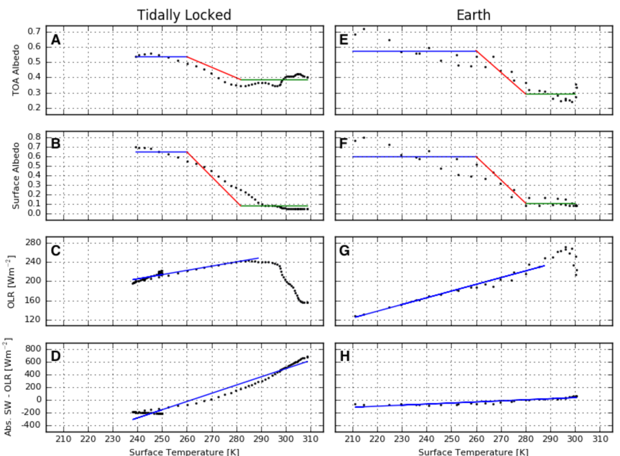
We infer effective EBM parameters by fitting the parameterizations used in the EBM to the example PlaSim simulations discussed in section 3.2.1. To do this we take the zonal mean of variables in the Earth configuration and the axial mean around the insolation axis in the tidally locked configuration (Koll & Abbot, 2015, 2016). The resulting parameters are displayed in Table 1 and the plots from which they are inferred are displayed in Figure 8. Figure 8 demonstrates that the fits are only approximate, as expected when fitting three-dimensional GCM results to a qualitative one-dimensional EBM. For example, the PlaSim albedo changes smoothly, rather than abruptly as in the EBM, between a high albedo in icy regions and a low albedo ice-free regions as a result of heterogeneities in clouds, land, snow, and the solar zenith angle (Figure 8A,B,E,F). The PlaSim outgoing longwave radiation is relatively linear in surface temperature only below 290-300 K (Figure 8C,G). Higher temperatures tend to be associated with deep convective clouds that significantly reduce the outgoing longwave radiation. Finally, the linearization of heat transport as a function of the surface temperature appears to be much better in the Earth configuration (Figure 8H) than in the tidally locked configuration (Figure 8D), where the heat transports are much larger and the night side has a fairly constant heat transport despite some variation in surface temperature.
Despite these limitations, the parameter values we infer for the Earth-like simulation are similar to those we used to obtain an Earth-like EBM simulation, which lends confidence to this methodology. Strikingly, we find that the effective value of , which represents atmospheric heat transport, is 7.6 times larger in tidally locked than in the Earth configuration (Table 1). As a result of the low rotation rate and strongly asymmetric stellar forcing, the tidally locked planet is significantly more efficient at transporting heat from the day to night side than Earth is at transporting heat from the equator to pole. This should tend to promote a snowball bifurcation. There is, however, a much smaller top-of-atmosphere ice/ocean albedo contrast in the tidally locked than the Earth configuration (Table 1), despite the fact that we use the Sun’s spectrum for both simulations. This results from strong cloud cover over the open ocean region in the tidally locked simulations (Figure 6J) and should tend to repress a snowball bifurcation. These two emergent properties of the PlaSim simulation therefore work in opposite directions.
If we simply plug our inferred tidally locked EBM parameters into the condition in Eq. (11), we find that it predicts that a snowball bifurcation should occur for a heat transport parameter above the critical value . From our tidally locked simulations we infer a heat transport parameter of (Table 1), yet PlaSim does not exhibit a snowball bifurcation in the tidally locked configuration (section 3.2.2). This underscores the fact that the EBM results should not be interpreted quantitatively. The EBM does, however, suggest that both the shape of the insolation and the decrease in ocean-ice albedo contrast as a result of cloud cover make a snowball bifurcation less likely in the tidally locked configuration, whereas the increase in the efficiency of heat transport makes a snowball bifurcation more likely.
| Parameter | Description | Tidally locked | Earth |
|---|---|---|---|
| lower TOA albedo | 0.4 | 0.3 | |
| upper TOA albedo | 0.55 | 0.55 | |
| lower surface albedo | 0.1 | 0.1 | |
| upper surface albedo | 0.65 | 0.6 | |
| OLR parameter | 0.9 W m-2 K-1 | 1.4 W m-2 K-1 | |
| heat transport parameter | 13.0 W m-2 K-1 | 1.7 W m-2 K-1 |
4 Discussion
An important implication of this work is that tidally locked planets in the habitable zone with a functioning silicate-weathering feedback (Walker et al., 1981) should not be able to exist in a snowball state for an extended period of time. If such a planet were somehow perturbed into a snowball state, weathering would shut down and the atmospheric CO2 would rise (Walker et al., 1981). With no snowball bifurcation and hysteresis, the planet would quickly warm enough to open up ocean at the substellar point or at continental margins if there were land at the substellar point. Further elaboration on this idea could be made using a coupled climate-weathering model. A snowball would only be possible for such a planet if it were located in the outer regions of the habitable zone and there was significant CO2 deposition on the night side. CO2 deposition has been calculated for Earth-like planets (Turbet et al., 2017), but not yet for tidally locked planets. Coincidentally, this implies that the location of the outer edge of the habitable zone is not well understood for tidally locked planets.
We only considered fully evolved tidally locked planets in a 1:1 spin-orbit state in this paper. Some M-star planets may be only partially tidally influenced (Leconte et al., 2015), or they could be trapped in higher order spin-eccentricity states (Wang et al., 2014). Considering the snowball bifurcation in other spin states would be an interesting topic of future research. A study of this issue would require global climate model simulations because many intermediate spin-orbit states lack a clear axis of symmetry to average around when using an EBM.
We found that the value of , the parameter governing horizontal heat transport in the EBM, helps determine whether a snowball bifurcation occurs for a tidally locked planet. The appropriate value of , which can be estimated from a GCM simulation, should be inversely proportional to planetary rotation rate (Williams & Kasting, 1997; Vallis & Farneti, 2009; Rose et al., 2017). Moreover, the value of necessary to cause a bifurcation (Eq. (11)) depends on the stellar spectrum because this affects the ice albedo (Joshi & Haberle, 2012; Shields et al., 2013, 2014). Both the stellar spectrum and the planetary rotation rate for a tidally locked planet receiving a given stellar flux depend on the mass of the M-dwarf. A topic of future work would therefore be to determine whether planets orbiting earlier M-dwarfs are more or less likely to exhibit a snowball bifurcation than those orbiting later M-dwarfs. In addition, many planetary parameters such as the atmospheric mass and the greenhouse gas complement will affect (as well as ) and could be explored in GCM simulations.
There has been a fair amount of recent work on the possibility of limit cycles between a snowball climate state and a warm climate state for planets in the habitable zone with a CO2 outgassing rate that is too low to maintain the warm climate state (Kadoya & Tajika, 2014; Menou, 2015; Haqq-Misra et al., 2016; Batalha et al., 2016; Abbot, 2016; Paradise & Menou, 2017). If tidally locked planets do not exhibit a snowball bifurcation, then they will not be subject to this type of climate limit cycle. Instead the planet would just comfortably settle into an Eyeball state.
Hu & Yang (2014) found that including a dynamic ocean causes the expansion of sea ice to be more sensitive to changes in the stellar flux. This motivates further research into the effect of ocean circulation on the snowball bifurcation for tidally locked planets. Since the ocean can transport heat in addition to the atmosphere, and since more heat transport makes a snowball bifurcation more likely, including a dynamic ocean could potentially make a snowball bifurcation more likely. But because ocean heat transport is a mechanical process and not a simple diffusive one, it may also lead to more complex bifurcation behavior with additional folds and stable states (Rose & Marshall, 2009; Ferreira et al., 2011; Pierrehumbert et al., 2011; Rose, 2015).
The substellar point in our simulations was located over the pacific ocean. We also tried aquaplanet simulations and achieved similar results. It would be interesting to test whether locating the substellar point over a large land mass such as Asia would significantly affects our results.
5 Conclusions
The main conclusions of this paper are:
-
1.
Tidally locked planets will not necessarily exhibit a snowball bifurcation. This is in contrast with planets with Earth-like rotation and orbit, which are required to exhibit a snowball bifurcation except in unrealistic edge cases.
-
2.
The reason tidally locked planets are not required to exhibit a snowball bifurcation is that the insolation increases strongly as the substellar point is approached.
-
3.
Whether a tidally locked planet actually does exhibit a snowball bifurcation depends on the heat transport and ice/ocean albedo contrast. Higher heat transport and a higher ice/ocean albedo contrast both favor a snowball bifurcation.
-
4.
We performed global climate model simulations that suggest that realistic tidally locked planets will not exhibit a snowball bifurcation. Although they should tend to have stronger heat transport, the top-of-atmosphere ice/ocean albedo contrast should tend to be smaller.
-
5.
This work suggests that we will not find habitable tidally locked exoplanets with an active carbon cycle in a snowball state. This should be verified with a model incorporating an active carbon cycle.
6 Acknowledgements
We thank Brian Rose for an excellent review. We acknowledge support from NASA grant number NNX16AR85G, which is part of the “Habitable Worlds” program and from the NASA Astrobiology Institutes Virtual Planetary Laboratory, which is supported by NASA under cooperative agreement NNH05ZDA001C. KM is supported by the Natural Sciences and Engineering Research Council of Canada.
Appendix A Artifact of Sea Ice Scheme
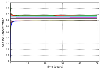
Interestingly and in contrast with Lucarini et al. (2013), we find a small separation between equilibrated states that were initialized from Warm and Cold Starts. The most likely reason Lucarini et al. (2013) did not observe this separation is that they started their Cold Start simulations from a significantly warmer climate state that was not globally glaciated. To further investigate this issue we show global mean sea ice concentration for a series of simulations with a stellar flux of 1200 W m-2 and initial conditions representing equilibrated climate states with different amounts of sea ice (Fig. 9). We find that states started within the apparent separation band are stable, rather than approaching separate stable warm and cold states at the upper and lower ends of the separation band. This means that the separation band actually represents a smeared state, which we can consider a continuum of states rather than two distinct “fixed points” with separate basins of attraction. This is clearly unrelated to a snowball bifurcation and does not alter our interpretation that there is no snowball bifurcation in PlaSim in the tidally locked configuration.
By further investigating the simulations that represent the continuum of states, we determined that the root cause of this behavior is the sea ice scheme, in which each grid cell must either be completely ice-covered or completely ice-free. A grid cell becomes completely ice-covered when the thickness of the sea ice in it exceeds m. The continuum of states is possible because within it an additional ocean grid cell can become ice-covered without leading to enough cooling in adjacent grid cells for them to become ice-covered as well. Therefore the climate is stable both with this additional grid box ice-covered and without it ice-covered. We tried to collapse the continuum of states from the PlaSim results into a single state by increasing the horizontal resolution, changing the ice thickness threshold for 100% ice coverage, removing continents, and adding ocean heat diffusion, but the continuum of states remained despite all of these modifications. The issue can therefore only be fully settled by simulations in a GCM that contains a more sophisticated sea ice scheme. Nevertheless we feel that our investigation has shown that the continuum of states in PlaSim in the tidally locked configuration is not related to a snowball bifurcation.
References
- Abbot (2016) Abbot, D. S. 2016, The Astrophysical Journal, 827, 117
- Abbot et al. (2011) Abbot, D. S., Voigt, A., & Koll, D. 2011, Journal of Geophysical Research, 116, D18103, doi:10.1029/2011JD015927
- Anglada-Escudé et al. (2016) Anglada-Escudé, G., Amado, P. J., Barnes, J., et al. 2016, Nature, 536, 437
- Barnes et al. (2016) Barnes, R., Deitrick, R., Luger, R., et al. 2016, arXiv preprint arXiv:1608.06919
- Batalha et al. (2016) Batalha, N. E., Kopparapu, R. K., Haqq-Misra, J., & Kasting, J. F. 2016, arXiv preprint arXiv:1609.00602
- Bitz et al. (2005) Bitz, C., Holland, M., Hunke, E., & Moritz, R. 2005, Journal of climate, 18, 2903
- Bolmont et al. (2017) Bolmont, E., Selsis, F., Owen, J. E., et al. 2017, Monthly Notices of the Royal Astronomical Society, 464, 3728
- Budyko (1969) Budyko, M. I. 1969, Tellus, 21, 611
- Dittmann et al. (2017) Dittmann, J. A., Irwin, J. M., Charbonneau, D., et al. 2017, Nature, 544, 333
- Donohoe & Battisti (2011) Donohoe, A., & Battisti, D. S. 2011, Journal of Climate, 24, 4402
- Ferreira et al. (2011) Ferreira, D., Marshall, J., & Rose, B. 2011, Journal of Climate, 24, 992
- Fraedrich et al. (2005) Fraedrich, K., Jansen, H., Kirk, E., Luksch, U., & Lunkeit, F. 2005, Meteorologische Zeitschrift, 14, 299
- Gillon et al. (2017) Gillon, M., Triaud, A. H., Demory, B.-O., et al. 2017, Nature, 542, 456
- Haqq-Misra et al. (2016) Haqq-Misra, J., Kopparapu, R. K., Batalha, N. E., Harman, C. E., & Kasting, J. F. 2016, arXiv preprint arXiv:1605.07130
- Hoffman et al. (1998) Hoffman, P. F., Kaufman, A. J., Halverson, G. P., & Schrag, D. P. 1998, Science, 281, 1342
- Hoffman & Schrag (2002) Hoffman, P. F., & Schrag, D. P. 2002, Terra Nova, 14, 129
- Hu & Yang (2014) Hu, Y., & Yang, J. 2014, Proceedings of the National Academy of Sciences, 111, 629
- Joshi et al. (1997) Joshi, M., Haberle, R., & Reynolds, R. 1997, Icarus, 129, 450
- Joshi & Haberle (2012) Joshi, M. M., & Haberle, R. M. 2012, Astrobiology, 12, 3
- Kadoya & Tajika (2014) Kadoya, S., & Tajika, E. 2014, The Astrophysical Journal, 790, 107
- Kasting et al. (1993) Kasting, J. F., Whitmire, D. P., & Reynolds, R. T. 1993, Icarus, 101, 108
- Kirschvink (1992) Kirschvink, J. 1992, in The Proterozoic Biosphere: A Multidisciplinary Study, ed. J. Schopf & C. Klein (Cambridge University Press, New York), 51–52
- Kite et al. (2011) Kite, E., Gaidos, E., & Manga, M. 2011, Astrophys Journal, 743, doi:10.1088/0004-637X/743/1/41
- Koll & Abbot (2015) Koll, D. D. B., & Abbot, D. S. 2015, The Astrophysical Journal, 802, 21, doi:10.1088/0004-637X/802/1/21
- Koll & Abbot (2016) —. 2016, The Astrophysical Journal, 825, 99
- Kopparapu et al. (2016) Kopparapu, R. K., Wolf, E. T., Haqq-Misra, J., et al. 2016, The Astrophysical Journal, 819, 84
- Laakso & Schrag (2014) Laakso, T. A., & Schrag, D. P. 2014, Earth and Planetary Science Letters, 388, 81
- Laakso & Schrag (2017) —. 2017, Geobiology, 15, 366
- Langen & Alexeev (2004) Langen, P. L., & Alexeev, V. A. 2004, Geophysical research letters, 31
- Leconte et al. (2013) Leconte, J., Forget, F., Charnay, B., et al. 2013, Astronomy & Astrophysics, 554, A69
- Leconte et al. (2015) Leconte, J., Wu, H., Menou, K., & Murray, N. 2015, Science, 347, 632
- Lucarini et al. (2013) Lucarini, V., Pascale, S., Boschi, R., Kirk, E., & Iro, N. 2013, Astronomische Nachrichten, 334, 576
- Meadows et al. (2016) Meadows, V. S., Arney, G. N., Schwieterman, E. W., et al. 2016, arXiv preprint arXiv:1608.08620
- Menou (2013) Menou, K. 2013, The Astrophysical Journal, 774, 51
- Menou (2015) —. 2015, Earth and Planetary Science Letters, 429, 20
- Merlis & Schneider (2010) Merlis, T. M., & Schneider, T. 2010, Journal of Advances in Modeling Earth Systems, 2, doi:10.3894/JAMES.2010.2.13
- North (1975) North, G. 1975, J Atmos Sci, 32, 1301
- Paradise & Menou (2017) Paradise, A., & Menou, K. 2017, arXiv preprint arXiv:1704.04535
- Pierrehumbert et al. (2011) Pierrehumbert, R., Abbot, D., Voigt, A., & Koll, D. 2011, Annual Review of Earth and Planetary Sciences, 39, 417
- Pierrehumbert (2011) Pierrehumbert, R. T. 2011, Astrophys J Lett, 726, L8, doi:10.1088/2041-8205/726/1/L8
- Ribas et al. (2016) Ribas, I., Bolmont, E., Selsis, F., et al. 2016, Astronomy & Astrophysics, 596, A111
- Roe & Baker (2010) Roe, G. H., & Baker, M. B. 2010, J Climate, 23, 4694, DOI:10.1175/2010JCLI3545.1
- Rose (2015) Rose, B. E. 2015, Journal of Geophysical Research: Atmospheres, 120, 1404
- Rose et al. (2017) Rose, B. E., Cronin, T. W., & Bitz, C. M. 2017, The Astrophysical Journal, submitted
- Rose & Marshall (2009) Rose, B. E., & Marshall, J. 2009, Journal of the Atmospheric Sciences, 66, 2828
- Salameh et al. (2017) Salameh, J., Popp, M., & Marotzke, J. 2017, Climate Dynamics, 1
- Segura et al. (2005) Segura, A., Kasting, J., Meadows, V., et al. 2005, Astrobiology, 5, 706
- Sellers (1969) Sellers, W. D. 1969, J of App Meteorology, 8, 392
- Shields et al. (2014) Shields, A. L., Bitz, C. M., Meadows, V. S., Joshi, M. M., & Robinson, T. D. 2014, The Astrophysical Journal Letters, 785, L9
- Shields et al. (2013) Shields, A. L., Meadows, V. S., Bitz, C. M., et al. 2013, Astrobiology, 13, 715
- Strogatz (1994) Strogatz, S. 1994, Nonlinear dynamics and chaos (Westview Press)
- Turbet et al. (2017) Turbet, M., Forget, F., Leconte, J., Charnay, B., & Tobie, G. 2017, arXiv preprint arXiv:1703.04624
- Turbet et al. (2016) Turbet, M., Leconte, J., Selsis, F., et al. 2016, Astronomy & Astrophysics, 596, A112
- Vallis & Farneti (2009) Vallis, G. K., & Farneti, R. 2009, Quarterly Journal of the Royal Meteorological Society, 135, 1643
- Voigt et al. (2011) Voigt, A., Abbot, D. S., Pierrehumbert, R. T., & Marotzke, J. 2011, Clim. Past, 7, 249, doi:10.5194/cp-7-249-2011
- Voigt & Marotzke (2010) Voigt, A., & Marotzke, J. 2010, Climate Dynamics, 35, 887, DOI:10.1007/s00382-009-0633-5
- Walker et al. (1981) Walker, J. C. G., Hays, P. B., & Kasting, J. F. 1981, Journal of Geophysical Research, 86, 9776
- Wang et al. (2014) Wang, Y., Tian, F., & Hu, Y. 2014, The Astrophysical Journal Letters, 791, L12
- Way et al. (2015) Way, M., Del Genio, A., Kelley, M., Aleinov, I., & Clune, T. 2015, arXiv preprint arXiv:1511.07283
- Williams & Kasting (1997) Williams, D. M., & Kasting, J. F. 1997, Icarus, 129, 254
- Winton (2003) Winton, M. 2003, Journal of climate, 16, 2875
- Wolf (2017) Wolf, E. T. 2017, The Astrophysical Journal Letters, 839, L1
- Wolf et al. (2017) Wolf, E. T., Shields, A. L., Kopparapu, R. K., Haqq-Misra, J., & Toon, O. B. 2017, The Astrophysical Journal, 837, 107
- Wordsworth et al. (2011) Wordsworth, R. D., Forget, F., Selsis, F., et al. 2011, Astrophys J Lett, 733, L48, doi:10.1088/2041-8205/733/2/L48
- Yang et al. (2013) Yang, J., Cowan, N. B., & Abbot, D. S. 2013, Astrophysical Journal Letters, 771, L45, DOI:10.1088/2041-8205/771/2/L45
- Yang et al. (2014) Yang, J., Liu, Y., Hu, Y., & Abbot, D. S. 2014, Astrophysical Journal Letters, 796, L22, doi:10.1088/2041-8205/796/2/L22
- Yang et al. (2012a) Yang, J., Peltier, W., & Hu, Y. 2012a, Journal of Climate, 25, 2711, doi: 10.1175/JCLI-D-11-00189.1
- Yang et al. (2012b) —. 2012b, Journal of Climate, 25, 2737, doi: 10.1175/JCLI-D-11-00190.1