Robust Block Preconditioners for Biot’s Model

Abstract

In this paper, we design robust and efficient block preconditioners for the two-field formulation of Biot’s consolidation model, where stabilized finite-element discretizations are used. The proposed block preconditioners are based on the well-posedness of the discrete linear systems. Block diagonal (norm-equivalent) and block triangular preconditioners are developed, and we prove that these methods are robust with respect to both physical and discretization parameters. Numerical results are presented to support the theoretical results.

1 Introduction

In this work, we study the quasi-static Biot’s model for soil consolidation. For linearly elastic, homogeneous, and isotropic porous medium, saturated by an incompressible Newtonian fluid, the consolidation is modeled by the following system of partial differential equations (see Biot1 ):

equilibrium equation: $$-{\rm div}\,\sigma^{\prime}+\alpha\nabla\,p={\bm{g}},\quad{\rm in}\,\Omega,$$ (1)

constitutive equation: $$\sigma^{\prime}=2\mu\varepsilon(\bm{u})+\lambda\operatorname{div}(\bm{u})I,\quad{\rm in}\,\Omega,$$ (2)

compatibility condition: $$\varepsilon({\bm{u}})=\frac{1}{2}(\nabla{\bm{u}}+\nabla{\bm{u}}^{t}),\quad{\rm in}\,\Omega,$$ (3)

Darcy’s law: $${\bm{w}}=-K\nabla p,\quad{\rm in}\,\Omega,$$ (4)

continuity equation: $$-\alpha\ {\operatorname{div}}\,\partial_{t}\bm{u}-{\operatorname{div}}\,{\bm{w}}=f,\quad{\rm in}\,\Omega,$$ (5)

where $\lambda$ and $\mu$ are the Lamé coefficients, $\alpha$ is the Biot-Willis constant (assumed to be one without loss of generality), $K$ is the hydraulic conductivity (ratio of the permeability of the porous medium to the viscosity of the fluid), $I$ is the identity tensor, ${\bm{u}}$ is the displacement vector, $p$ is the pore pressure, $\sigma^{\prime}$ and $\varepsilon$ are the effective stress and strain tensors for the porous medium, and ${\bm{w}}$ is the percolation velocity of the fluid relative to the soil. The right-hand-side term, ${\bm{g}}$, is the density of applied body forces and the source term $f$ represents a forced fluid extraction or injection process. Here, we consider a bounded open subset, $\Omega\subset{\mathbb{R}}^{d},\;d=2,3$ with regular boundary $\Gamma$.

Suitable discretizations yield a large-scale linear system of equations to solve at each time step, which are typically ill-conditioned and difficult to solve in practice. Thus, iterative solution techniques are usually considered. For the coupled poromechanics equations considered here, there are two typical approaches: fully-coupled or monolithic methods and iterative coupling methods. Monolithic techniques solve the resulting linear system simultaneously for all the involved unknowns. In this context, efficient preconditioners are developed to accelerate the convergence of Krylov subspace methods and special smoothers are designed in a multigrid framework. Examples of this approach for poromechanics is found in Bergamaschi2007 ; Ferronato2010 ; Gaspar2004 ; Luo2017 ; Gaspar2017sub ; Lee.J;Mardal.K;Winther.R2017a ; Baerland.T;Lee.J;Mardal.K;Winther.R2017a and the references therein. Iterative coupling Kim.J;Tchelepi.H;Juanes.R;others2009a ; Kim_PhD , in contrast, is a sequential approach in which either the fluid flow problem or the geomechanics part is solved first, followed by the solution of the other system. This process is repeated until a converged solution within a prescribed tolerance is achieved. The main advantage of iterative coupling methods is that existing software for simulating fluid flow and geomechanics can be reused. These type of schemes have been widely studied Mikelic.A;Wheeler.M2013a ; Both2017 ; Almani ; Bause . In particular, in Castelleto2015 and White.J;Castelletto.N;Tchelepi.H2016a a re-interpretation of the four commonly used sequential splitting methods as preconditioned-Richardson iterations with block-triangular preconditioning is presented. Such analysis indicates that a fully-implicit method outperforms the convergence rate of the sequential-implicit methods. Following this idea a family of preconditioners to accelerate the convergence of Krylov subspace methods was recently proposed for the three-field formulation of the poromechanics problem Castelleto2016 .

In this work, we take the monolithic approach and develop efficient block preconditoners for Krylov subspace methods for solving the linear systems of equations arising from the discretization of the two-field formulation of Biot’s model. These preconditioners take advantage of the block structure of the discrete problem, decoupling different fields at the preconditioning stage. Our theoretical results show their efficiency and robustness with respect to the physical and discretization parameters. Moreover, the techniques proposed here can also be used for designing fast solvers for the three-field formulation of the Biot’s model.

The paper is organized as follows. Section 2 introduces the stabilized finite-element discretizations for the two-field formulation and the basics of block preconditioners. The proposed block preconditioners are introduced in Section 3. Finally, in Section 4, we present numerical experiments illustrating the effectiveness and robustness of the proposed preconditioners and make concluding remarks in Section 5.

2 Two-Field Formulation

First, we consider the two-field formulation of Biot’s model (1)-(5), where the unknowns are the displacement $\bm{u}$ and the pressure $p$. By considering apropriate Sobolev spaces and integration by parts, we have the following variational form: find $\bm{u}(t)\in\bm{H}_{0}^{1}(\Omega)$ and $p(t)\in H_{0}^{1}(\Omega)$, such that

$$a(\bm{u},\bm{v})-\alpha(\operatorname{div}\bm{v},p)=(\bm{g},\bm{v}),\quad\forall\bm{v}\in\bm{H}_{0}^{1}(\Omega),$$ (6)

$$-\alpha(\operatorname{div}\partial_{t}\bm{u},q)-a_{p}(p,q)=(f,q),\quad\forall q\in H_{0}^{1}(\Omega),$$ (7)

where

$$a(\bm{u},\bm{v}) =2\mu\int_{\Omega}\varepsilon(\bm{u}):\varepsilon(\bm{v})+\lambda\int_{\Omega}\operatorname{div}\bm{u}\operatorname{div}\bm{v}\quad\text{and}\quad a_{p}(p,q) =\int_{\Omega}K\nabla p\cdot\nabla q.$$

The system is completed with suitable initial data $\bm{u}(0)$ and $p(0)$.

2.1 Finite-Element Method

We consider two stable discretizations for the two-field formulation of Biot’s model proposed in Rodrigo.C;Gaspar.F;Hu.X;Zikatanov.L2016a : $\mathbb{P}_{1}$-$\mathbb{P}_{1}$ elements and the Mini element with stabilization. The fully discretized scheme at time $t_{n}$, $n=1,2,\dots$ is as follows:
Find $\bm{u}_{h}^{n}\in\bm{V_{h}}\subset\bm{H}^{1}_{0}(\Omega)$ and $p_{h}^{n}\in Q_{h}\subset H^{1}_{0}(\Omega)$, such that,

$$a(\bm{u}_{h}^{n},\bm{v}_{h})-\alpha(\operatorname{div}\bm{v}_{h},p_{h}^{n})=(\bm{g}(t_{n}),\bm{v}_{h}),\quad\forall\bm{v}_{h}\in\bm{V}_{h},$$ (8)

$$-\alpha(\operatorname{div}\bar{\partial}_{t}\bm{u}_{h}^{n},q_{h})-a_{p}(p_{h}^{n},q_{h})-\eta h^{2}(\nabla\bar{\partial}_{t}p^{n}_{h},\nabla q_{h})=(f(t_{n}),q_{h}),\quad\forall q_{h}\in Q_{h},$$ (9)

where $\bar{\partial}_{t}\bm{u}_{h}^{n}:=(\bm{u}_{h}^{n}-\bm{u}_{h}^{n-1})/\tau$, $\bar{\partial}_{t}p_{h}^{n}:=(p_{h}^{n}-p_{h}^{n-1})/\tau$, and $\eta$ represents the stabilization parameter. Here, $\bm{V}_{h}$ and $Q_{h}$ come from the $\mathbb{P}_{1}$-$\mathbb{P}_{1}$ or Mini element. At each time step, the linear system has the following two-by-two block form:

$$\mathcal{A}\bm{x}=\bm{b},\quad\mathcal{A}=\begin{pmatrix}A_{\bm{u}}&~{}&\alpha B^{T}\\ \alpha B&~{}&-\tau A_{p}-\eta h^{2}L_{p}\end{pmatrix},\ \bm{x}=\begin{pmatrix}\bm{u}\\ p\end{pmatrix},\ \text{and}\ \bm{b}=\begin{pmatrix}\bm{f}_{\bm{u}}\\ f_{p}\end{pmatrix},$$ (10)

where $a(\bm{u},\bm{v})\rightarrow A_{\bm{u}}$, $-(\operatorname{div}\bm{u},q)\rightarrow B$, $a_{p}(\nabla p,\nabla q)\rightarrow A_{p}$, and $(\nabla p,\nabla q)\rightarrow L_{p}$ represent the discrete versions of the variational forms.

2.2 Block Preconditioners

Next, we introduce the general theory for designing block preconditioners of Krylov subspace iterative methods Loghin.D;Wathen.A2004 ; Mardal.K;Winther.R2010 . Let $\bm{X}$ be a real, separable Hilbert space equipped with norm $\|\cdot\|_{\bm{X}}$ and inner product $(\cdot,\cdot)_{\bm{X}}$. Also let $\mathcal{A}:\bm{X}\mapsto\bm{X}^{\prime}$ be a bounded and symmetric operator induced by a symmetric and bounded bilinear form $\mathcal{L}(\cdot,\cdot)$, i.e. $\langle\mathcal{A}\bm{x},\bm{y}\rangle=\mathcal{L}(\bm{x},\bm{y})$. We assume the bilinear form is bounded and satisfies an inf-sup condition:

$$|\mathcal{L}(\bm{x},\bm{y})|\leq\beta\|\bm{x}\|_{\bm{X}}\|\bm{y}\|_{\bm{X}},\ \forall\bm{x},\bm{y}\in\bm{X}\quad\mbox{and}\quad\inf_{\bm{x}\in\bm{X}}\sup_{\bm{y}\in\bm{X}}\frac{\mathcal{L}(\bm{x},\bm{y})}{\|\bm{x}\|_{\bm{X}}\|\bm{y}\|_{\bm{X}}}\geq\gamma>0.$$ (11)

Norm-equivalent Preconditioner

Consider a symmetric positive definite (SPD) operator $\mathcal{M}:\bm{X}^{\prime}\mapsto\bm{X}$ as a preconditioner for solving $\mathcal{A}\bm{x}=\bm{b}$. We define an inner product $(\bm{x},\bm{y})_{\mathcal{M}^{-1}}:=\langle\mathcal{M}^{-1}\bm{x},\bm{y}\rangle$ on $\bm{X}$ and the corresponding induced norm is $\|\bm{x}\|^{2}_{\mathcal{M}^{-1}}:=(\bm{x},\bm{x})_{\mathcal{M}^{-1}}$. It is easy to show that $\mathcal{MA}:\bm{X}\mapsto\bm{X}$ is symmetric with respect to $(\cdot,\cdot)_{\mathcal{M}^{-1}}$. Therefore, we can use $\mathcal{M}$ as a preconditioner for the MINRES algorithm and use the following theorem for the convergence rate of preconditioned MINRES.

Theorem 2.1

Greenbaum.A.1997a If $\bm{x}^{m}$ is the $m$-th iteration of MINRES and $\bm{x}$ is the exact solution, then,

$$\|\bm{r}^{m}\|_{\mathcal{M}}\leq 2\rho^{m}\|\bm{r}^{0}\|_{\mathcal{M}},\quad$$ (12)

where $\bm{r}^{k}=\mathcal{A}(x-x^{k})$ is the residual after the $k$-th iteration, $\rho=\frac{\kappa(\mathcal{MA})-1}{\kappa(\mathcal{MA})+1}$, and $\kappa(\mathcal{MA})$ denotes the condition number of $\mathcal{MA}$.

In Mardal.K;Winther.R2010 , Mardal and Winther show that, if the well-posedness conditions, (11), hold, and $\mathcal{M}$ satisfies

$$c_{1}\|\bm{x}\|_{\bm{X}}^{2}\leq\|\bm{x}\|_{\mathcal{M}^{-1}}^{2}\leq c_{2}\|\bm{x}\|_{\bm{X}}^{2},$$ (13)

then, $\mathcal{A}$ and $\mathcal{M}$ are norm-equivalent and $\kappa(\mathcal{MA})\leq\frac{c_{2}\beta}{c_{1}\gamma}$. This implies that $\rho\leq\frac{c_{2}\beta-c_{1}\gamma}{c_{2}\beta+c_{1}\gamma}$. Thus, if the original problem is well-posed and the constants $c_{1}$ and $c_{2}$ are independent of the physical and discretization parameters, then the convergence rate of preconditioned MINRES is uniform, hence $\mathcal{M}$ is a robust preconditioner.

FOV-equivalent Preconditioner

In this section we consider the class of field-of-values-equivalent (FOV-equivalent) preconditioners $\mathcal{M}_{L}:\bm{X}^{\prime}\mapsto\bm{X}$, for GMRES. We define the notion of FOV-equivalence after the following classical theorem on the convergence rate of the preconditioned GMRES method.

Theorem 2.2

Elman.H1982a ; Eisenstat.S;Elman.H;Schultz.M1983b If $\bm{x}^{m}$ is the $m$-th iteration of the GMRES method preconditioned with $\mathcal{M}_{L}$ and $\bm{x}$ is the exact solution, then

$$\|\mathcal{M}_{L}\mathcal{A}(\bm{x}-\bm{x}^{m})\|^{2}_{\mathcal{M}^{-1}}\leq\left(1-\frac{\Sigma^{2}}{\Upsilon^{2}}\right)^{m}\|\mathcal{M}_{L}\mathcal{A}(\bm{x}-\bm{x}^{0})\|^{2}_{\mathcal{M}^{-1}},$$ (14)

where, for any $\bm{x}\in\bm{X}$,

$$\Sigma\leq\frac{(\mathcal{M}_{L}\mathcal{A}\bm{x},\bm{x})_{\mathcal{M}^{-1}}}{(\bm{x},\bm{x})_{\mathcal{M}^{-1}}},\quad\frac{\|\mathcal{M}_{L}\mathcal{A}\bm{x}\|_{\mathcal{M}^{-1}}}{\|\bm{x}\|_{\mathcal{M}^{-1}}}\leq\Upsilon.$$ (15)

If the constants $\Sigma$ and $\Upsilon$ are independent of the physical and discretization parameters, then $\mathcal{M}_{L}$ is a uniform left preconditioner for GMRES and is referred to as an FOV-equivalent preconditioner. In Loghin.D;Wathen.A2004 , a block lower triangular preconditioner has been shown to satisfy (15) based on the well-posedness conditions, (11), for Stokes/Navier-Stokes equations. More recently, the same approach has been generalized to Maxwell’s equations Adler.J;Hu.X;Zikatanov.L2017a and Magnetohydrodynamics Ma.Y;Hu.K;Hu.X;Xu.J2016a .

Similar arguments also apply to right preconditioners for GMRES, $\mathcal{M}_{U}:\bm{X}^{\prime}\mapsto\bm{X}$, where the operators, $\mathcal{M}_{U}$ and $\mathcal{A}$, are FOV equivalent if, for any $\bm{x}^{\prime}\in\bm{X}^{\prime}$,

$$\Sigma\leq\frac{(\mathcal{A}\mathcal{M}_{U}\bm{x}^{\prime},\bm{x}^{\prime})_{\mathcal{M}}}{(\bm{x}^{\prime},\bm{x}^{\prime})_{\mathcal{M}}},\quad\frac{\|\mathcal{A}\mathcal{M}_{U}\bm{x^{\prime}}\|_{\mathcal{M}}}{\|\bm{x}^{\prime}\|_{\mathcal{M}}}\leq\Upsilon.$$ (16)

Again, if $\Sigma$ and $\Upsilon$ are independent of the physical and discretization parameters, $\mathcal{M}_{U}$ is a uniform right preconditioner for GMRES. Such an approach leads to block upper triangular preconditioners.

3 Robust Preconditioners for Biot’s Model

In this section, following the framework proposed in Loghin.D;Wathen.A2004 ; Mardal.K;Winther.R2010 and techniques recently developed in Ma.Y;Hu.K;Hu.X;Xu.J2016a , we design block diagonal and triangular preconditioners based on the well-posedness of the discretized linear system at each time step. First, we study the well-posedness of the linear system (10). The analysis here is similar to the analysis in Rodrigo.C;Gaspar.F;Hu.X;Zikatanov.L2016a . However, we make sure that the constants arising from the analysis are independent of any physical and discretization parameters.

The choice of finite-element spaces give $\bm{X}=\bm{V}_{h}\times Q_{h}$, and the finite-element pair satisfies the following inf-sup condition,

$$\sup_{\bm{v}\in\bm{V}_{h}}\frac{(\operatorname{div}\bm{v},q)}{\|\bm{v}\|_{1}}\geq\gamma^{0}_{B}\|q\|-\xi^{0}h\|\nabla q\|,\quad\forall\,q\in Q_{h}.$$ (17)

Here, $\gamma_{B}^{0}>0$ and $\xi^{0}\geq 0$ are constants that do not depend on the mesh size. Moreover, if we use the Mini-element, $\xi^{0}=0$.

For $\bm{x}=(\bm{u},p)^{T}$, we define the following norm,

$$\|\bm{x}\|^{2}_{\bm{X}}:=\|\bm{u}\|^{2}_{A_{\bm{u}}}+\tau\|p\|_{A_{p}}^{2}+\eta h^{2}\|p\|_{L_{p}}^{2}+\frac{\alpha^{2}}{\zeta^{2}}\|p\|^{2},$$ (18)

where $\|\bm{u}\|^{2}_{A_{\bm{u}}}:=a(\bm{u},\bm{u})$, $\|p\|^{2}_{A_{p}}:=a_{p}(\nabla p,\nabla p)$, $\|p\|^{2}_{L_{p}}:=(\nabla p,\nabla p)$, $\zeta=\sqrt{\lambda+\frac{2\mu}{d}}$, and $d=2$ or $3$ is the dimension of the problem. With $\zeta$ defined above, we have $\|\bm{v}\|_{A_{\bm{u}}}\leq\sqrt{d}\zeta\|\bm{v}\|_{1}$, and can reformulate the inf-sup condition, (17), as follows,

$$\sup_{\bm{v}\in\bm{V}_{h}}\frac{(B\bm{v},q)}{\|\bm{v}\|_{A_{\bm{u}}}}\geq\sup_{\bm{v}\in\bm{V}_{h}}\frac{(B\bm{v},q)}{\sqrt{d}\zeta\|\bm{v}\|_{1}}\geq\frac{\gamma_{B}^{0}}{\sqrt{d}\zeta}\|q\|-\frac{\xi^{0}}{\sqrt{d}\zeta}h\|\nabla q\|=:\frac{\gamma_{B}}{\zeta}\|q\|-\frac{\xi}{\zeta}h\|\nabla q\|,$$ (19)

where $\gamma_{B}:=\gamma_{B}^{0}/\sqrt{d}$ and $\xi=\xi^{0}/\sqrt{d}$.

Noting that for $d=2,3$, $2\mu(\varepsilon(\bm{v}),\varepsilon(\bm{v}))\leq a(\bm{v},\bm{v})\leq(2\mu+d\lambda)(\varepsilon(\bm{v}),\varepsilon(\bm{v}))$. Thus, $(\operatorname{div}\bm{v},\operatorname{div}\bm{v})\leq d(\varepsilon(\bm{v}),\varepsilon(\bm{v}))$ and,

$$\zeta^{2}\|B\bm{v}\|^{2}=(\lambda+\frac{2\mu}{d})\|\operatorname{div}\bm{v}\|^{2}\leq\|\bm{v}\|^{2}_{A_{\bm{u}}}\Longrightarrow\|B\bm{v}\|\leq\frac{1}{\zeta}\|\bm{v}\|_{A_{\bm{u}}}.$$ (20)

This allows us to show that linear system (10) is well-posed.

Theorem 3.1

For $\bm{x}=(\bm{u},p)$ and $\bm{y}=(\bm{v},q)$, let

$$\mathcal{L}(\bm{x},\bm{y})=(A_{\bm{u}}\bm{u},\bm{v})+\alpha(B\bm{v},p)+\alpha(B\bm{u},q)-\tau(K\nabla p,\nabla q)-\eta h^{2}(\nabla p,\nabla q).$$ (21)

Then, (11) holds and $\mathcal{A}$ defined in (10) is an isomorphism from $\bm{X}$ to $\bm{X}^{\prime}$ provided the stabilization parameter $\eta=\delta\frac{\alpha^{2}}{\zeta^{2}}$ with $\delta>0$. Moreover, the constants $\gamma$ and $\beta$ are independent of the physical and discretization parameters.

Proof

Based on the inf-sup condition (17) and (19), for any $p$, there exist $\bm{w}\in\bm{V}_{h}$ such that $(B\bm{w},p)\geq\left(\frac{\gamma_{B}}{\zeta}\|p\|-\frac{\xi}{\zeta}h\|\nabla p\|\right)\|\bm{w}\|_{A_{\bm{u}}}$ and $\|\bm{w}\|_{A_{\bm{u}}}=\|p\|$. For given $(\bm{u},p)\in\bm{V}_{h}\times Q_{h}$, we choose $\bm{v}=\bm{u}+\theta\bm{w}$, $\theta=\vartheta\frac{\gamma_{B}\alpha}{\zeta}$ and $q=-p$ and then have,

$$\mathcal{L}(\bm{x},\bm{y}) =(A_{\bm{u}}\bm{u},\bm{u}+\theta\bm{w})+\alpha(B(\bm{u}+\theta\bm{w}),p)-\alpha(B\bm{u},p)$$

$$\quad+\tau(K\nabla p,\nabla p)+\eta h^{2}(\nabla p,\nabla p)$$

$$\geq\|\bm{u}\|^{2}_{A_{\bm{u}}}-\vartheta\|\bm{u}\|_{A_{\bm{u}}}\frac{\gamma_{B}\alpha}{\zeta}\|p\|+\vartheta\frac{\gamma_{B}^{2}\alpha^{2}}{\zeta^{2}}\|p\|^{2}-\vartheta\frac{\gamma_{B}\alpha^{2}}{\zeta^{2}}\xi h\|\nabla p\|\|p\|$$

$$\quad+\tau\|p\|^{2}_{A_{p}}+\frac{\delta}{\xi^{2}}\frac{\alpha^{2}}{\zeta^{2}}\xi^{2}h^{2}\|\nabla p\|^{2}$$

$$\geq\begin{pmatrix}\|\bm{u}\|_{A_{\bm{u}}}\\ \frac{\gamma_{B}\alpha}{\zeta}\|p\|\\ \frac{\alpha}{\zeta}\xi h\|\nabla p\|\\ \sqrt{\tau}\|p\|_{A_{p}}\end{pmatrix}^{T}\begin{pmatrix}1&-\vartheta/2&0&0\\ -\vartheta/2&\vartheta&-\vartheta/2&0\\ 0&-\vartheta/2&\delta/\xi^{2}&0\\ 0&0&0&1\end{pmatrix}\begin{pmatrix}\|\bm{u}\|_{A_{\bm{u}}}\\ \frac{\gamma_{B}\alpha}{\zeta}\|p\|\\ \frac{\alpha}{\zeta}\xi h\|\nabla p\|\\ \sqrt{\tau}\|p\|_{A_{p}}\end{pmatrix}.$$

If $0<\vartheta<\min\{2,\frac{2\delta}{\xi^{2}}\}$, the matrix in the middle is SPD and there exists $\gamma_{0}$ such that

$$\mathcal{L}(\bm{x},\bm{y}) \geq\gamma_{0}\left(\|\bm{u}\|^{2}_{A_{\bm{u}}}+\frac{\gamma^{2}_{B}\alpha^{2}}{\zeta^{2}}\|p\|^{2}+\frac{\alpha^{2}}{\zeta^{2}}\xi^{2}h^{2}\|\nabla p\|^{2}+\tau\|p\|^{2}_{A_{p}}\right)\geq\tilde{\gamma}\|\bm{x}\|_{\bm{X}}^{2},$$

where $\tilde{\gamma}=\gamma_{0}\min\{\gamma_{B}^{2},\xi^{2}/\delta\}$. Also, it is straightforward to verify $\|(\bm{v},q)\|_{\bm{X}}^{2}\leq\bar{\gamma}^{2}\|(\bm{u},p)\|_{\bm{X}}^{2}$, and the boundedness of $\mathcal{L}$ by continuity of each term and the Cauchy-Schwarz inequality. Therefore, $\mathcal{L}$ satisfies (11) with $\gamma=\tilde{\gamma}/\bar{\gamma}$.

Remark 1

Note that the choice of $\zeta=\sqrt{\lambda+2\mu/d}$ is essential to the proof, but is consistent with previous practical choice in implementations Aguilar2008 ; Rodrigo.C;Gaspar.F;Hu.X;Zikatanov.L2016a . Additionally, choosing any $\delta>0$ is sufficient to show the well-posedness of the stabilized discretization. However, for eliminating non-physical oscillations of the pressure approximation seen in practice Aguilar2008 , this is not sufficient, and $\delta$ should be sufficiently large. For example, in 1D, we choose $\delta=1/4$.

3.1 Block Diagonal Preconditioner

Now that we have shown (11) and that the system is well-posed, we find SPD operators such that (13) is satisfied. One natural choice is the Reisz operator corresponding to the inner product $(\cdot,\cdot)_{\bm{X}}$, $(\mathcal{B}\bm{f},\bm{x})_{\bm{X}}=\langle\bm{f},\bm{x}\rangle,\ \forall\bm{f}\in\bm{X}^{\prime},\ \bm{x}\in\bm{X}.$ For the two-field stabilized discretization and the norm $\|\cdot\|_{\bm{X}}$ defined in (18), we get

$$\mathcal{B}_{D}=\begin{pmatrix}A_{\bm{u}}&0\\ 0&\tau A_{p}+\eta h^{2}L_{p}+\frac{\alpha^{2}}{\zeta^{2}}M\end{pmatrix}^{-1},$$ (22)

where $M$ is the mass matrix of the pressure block. Since $\mathcal{B}_{D}$ satisfies the norm-equivalent condition with $c_{1}=c_{2}=1$, by Theorem 3.1, we have $\kappa(\mathcal{B}_{D}\mathcal{A})=\mathcal{O}(1)$.

In practice, applying the preconditioner $\mathcal{B}_{D}$ involves the action of inverting the diagonal blocks exactly, which is very expensive and infeasible. Therefore, we replace the diagonal blocks by their spectral equivalent SPD approximations,

$$\mathcal{M}_{D}=\begin{pmatrix}H_{\bm{u}}&0\\ 0&H_{p}\end{pmatrix},$$

where

$$c_{1,\bm{u}}(H_{\bm{u}}\bm{u},\bm{u})\leq(A_{\bm{u}}^{-1}\bm{u},\bm{u})\leq c_{2,\bm{u}}(H_{\bm{u}}\bm{u},\bm{u})$$ (23)

$$c_{1,p}(H_{p}p,p)\leq((\tau A_{p}+\eta h^{2}L_{p}+\frac{\alpha^{2}}{\zeta^{2}}M)^{-1}p,p)\leq c_{2,p}(H_{p}p,p).$$ (24)

Again, $\mathcal{M}_{D}$ and $\mathcal{A}$ are norm-equivalent and $\kappa(\mathcal{M}_{D}\mathcal{A})=\mathcal{O}(1)$ by Theorem 3.1.

3.2 Block Triangular Preconditioners

Next, we consider block triangular preconditioners for the stabilized scheme, $\mathcal{A}$. For simplicity of the analysis, we modify $\mathcal{A}$ slightly by negating the second equation.

We consider two kinds of block triangular preconditioners,

$$\mathcal{B}_{L}=\begin{pmatrix}A_{\bm{u}}&0\\ -\alpha B&\tau A_{p}+\eta h^{2}L_{p}+\frac{\alpha^{2}}{\zeta^{2}}M\end{pmatrix}^{-1}\ \text{and}\ \mathcal{M}_{L}=\begin{pmatrix}H_{\bm{u}}^{-1}&0\\ -\alpha B&H_{p}^{-1}\end{pmatrix}^{-1},$$ (25)

and block upper triangular preconditioners,

$$\mathcal{B}_{U}=\begin{pmatrix}A_{\bm{u}}&\alpha B^{T}\\ 0&\tau A_{p}+\eta h^{2}L_{p}+\frac{\alpha^{2}}{\zeta^{2}}M\end{pmatrix}^{-1}\ \text{and}\ \mathcal{M}_{U}=\begin{pmatrix}H_{\bm{u}}^{-1}&\alpha B^{T}\\ 0&H_{p}^{-1}\end{pmatrix}^{-1}.$$ (26)

According to Theorem 2.2, we need to show those block preconditioners satisfies the FOV-equivalence, (15) and (16). We first consider the block lower triangular preconditioner, $\mathcal{B}_{L}$.

Theorem 3.2

There exists constants $\Sigma$ and $\Upsilon$, independent of discretization or physical parameters, such that, for any $\bm{x}=(\bm{u},p)^{T}\neq\bm{0}$,

$$\Sigma\leq\frac{(\mathcal{B}_{L}\mathcal{A}\bm{x},\bm{x})_{(\mathcal{B}_{D})^{-1}}}{(\bm{x},\bm{x})_{(\mathcal{B}_{D})^{-1}}},\ \frac{\|\mathcal{B}_{L}\mathcal{A}\bm{x}\|_{(\mathcal{B}_{D})^{-1}}}{\|\bm{x}\|_{(\mathcal{B}_{D})^{-1}}}\leq\Upsilon,$$

provided that $\eta=\delta\frac{\alpha^{2}}{\zeta^{2}}$ with $\delta>0$.

Proof

By direct computation, we have

$$(\mathcal{B}_{L}\mathcal{A}\bm{x},\bm{x})_{(\mathcal{B}_{D})^{-1}} =(\bm{u},\bm{u})_{A_{\bm{u}}}+\alpha(B^{T}p,\bm{u})+\tau(p,p)_{A_{p}}$$

$$\quad+\eta h^{2}(L_{p}p,p)+\alpha^{2}(BA_{\bm{u}}^{-1}B^{T}p,p)$$

$$\geq\Sigma_{0}\left(\|\bm{u}\|_{A_{\bm{u}}}^{2}+\tau\|p\|_{A_{p}}^{2}+\eta h^{2}\|p\|_{L_{p}}^{2}+\alpha^{2}\|B^{T}p\|^{2}_{A_{\bm{u}}^{-1}}\right).$$

Note that, due to the inf-sup condition (17),

$$\|B^{T}p\|_{A_{\bm{u}}^{-1}}=\sup_{\bm{v}}\frac{(B\bm{v},p)}{\|\bm{v}\|_{A_{\bm{u}}}}\geq\frac{\gamma_{B}}{\zeta}\|p\|-\frac{\xi}{\zeta}h\|\nabla p\|.$$

Therefore, since $\eta=\delta\frac{\alpha^{2}}{\zeta^{2}}$ with $\delta>0$ and by choosing $\frac{1}{1+\delta/\xi^{2}}<\theta<1$, we have,

$$(\mathcal{B}_{L}\mathcal{A}\bm{x},\bm{x})_{(\mathcal{B}_{D})^{-1}} \geq\Sigma_{0}\left[\|\bm{u}\|_{A_{\bm{u}}}^{2}+\tau\|p\|_{A_{p}}^{2}+\eta h^{2}\|p\|_{L_{p}}^{2}\right.$$

$$\quad\left.+\alpha^{2}\left(\frac{\gamma_{B}}{\zeta}\|p\|-\frac{\xi}{\zeta}h\|\nabla p\|\right)^{2}\right]$$

$$\geq\Sigma_{0}\left[\|\bm{u}\|_{A_{\bm{u}}}^{2}+\tau\|p\|_{A_{p}}^{2}\right.$$

$$\quad\left.+(1-\theta)\frac{\gamma_{B}^{2}\alpha^{2}}{\zeta^{2}}\|p\|^{2}+\left(1+\frac{\delta}{\xi^{2}}-\frac{1}{\theta}\right)\frac{\alpha^{2}}{\zeta^{2}}\xi^{2}h^{2}\|\nabla p\|^{2}\right]$$

$$\geq\Sigma_{0}\Sigma_{1}\left(\|\bm{u}\|_{A_{\bm{u}}}^{2}+\tau\|p\|_{A_{p}}^{2}+\frac{\alpha^{2}}{\zeta^{2}}h^{2}\|p\|_{L_{p}}^{2}+\frac{\alpha^{2}}{\zeta^{2}}\|p\|^{2}\right)$$

$$=:\Sigma(\bm{x},\bm{x})_{(\mathcal{B}_{D})^{-1}},$$

where $\Sigma_{1}:=\min\{1,(1-\theta)\gamma_{B}^{2},\left(1+\frac{\delta}{\xi^{2}}-\frac{1}{\theta}\right)\frac{\xi^{2}}{\delta}\}$. This gives the lower bound. The upper bound $\Upsilon$ can be obtain directly from the continuity of each term, the Cauchy-Schwarz inequality, and the fact that $\|B^{T}p\|_{A_{\bm{u}}^{-1}}\leq\frac{1}{\zeta}\|p\|$ obtained by (20).

Similarly, we can show that the other three block preconditioners are also FOV-equivalent with $\mathcal{A}$ and, therefore, can be used as preconditioners for GMRES. Due to the length constraint of this paper and the fact that the proofs are similar, we only state the results here.

Theorem 3.3

If the conditions (23) and (24) hold and $\|I-H_{\bm{u}}A_{\bm{u}}\|_{A_{\bm{u}}}\leq\rho$ with $0\leq\rho<1$, and there exists constants $\Sigma$ and $\Upsilon$, independent of discretization or physical parameters, such that, for any $\bm{x}=(\bm{u},p)^{T}\neq\bm{0}$, we have

$$\Sigma\leq\frac{(\mathcal{M}_{L}\mathcal{A}\bm{x},\bm{x})_{(\mathcal{M}_{D})^{-1}}}{(\bm{x},\bm{x})_{(\mathcal{M}_{D})^{-1}}},\ \frac{\|\mathcal{M}_{L}\mathcal{A}\bm{x}\|_{(\mathcal{M}_{D})^{-1}}}{\|\bm{x}\|_{(\mathcal{M}_{D})^{-1}}}\leq\Upsilon,$$

provided that $\eta=\delta\frac{\alpha^{2}}{\zeta^{2}}$ with $\delta>0$.

Theorem 3.4

There exists constants $\Sigma$ and $\Upsilon$, independent of discretization or physical parameters, such that, for any $\bm{0}\neq\bm{x}^{\prime}\in\bm{X}^{\prime}$, we have

$$\Sigma\leq\frac{(\mathcal{A}\mathcal{B}_{U}\bm{x}^{\prime},\bm{x}^{\prime})_{\mathcal{B}_{D}}}{(\bm{x}^{\prime},\bm{x}^{\prime})_{\mathcal{B}_{D}}},\ \frac{\|\mathcal{A}\mathcal{B}_{U}\bm{x}^{\prime}\|_{\mathcal{B}_{D}}}{\|\bm{x}^{\prime}\|_{\mathcal{B}_{D}}}\leq\Upsilon,$$

provided that $\eta=\delta\frac{\alpha^{2}}{\zeta^{2}}$ with $\delta>0$.

Theorem 3.5

If the conditions (23) and (24) hold and $\|I-H_{\bm{u}}A_{\bm{u}}\|_{A_{\bm{u}}}\leq\rho$ with $0\leq\rho<1$, and there exists constants $\Sigma$ and $\Upsilon$, independent of discretization or physical parameters, such that, for any $\bm{0}\neq\bm{x}^{\prime}\in\bm{X}^{\prime}$, we have

$$\Sigma\leq\frac{(\mathcal{A}\mathcal{M}_{U}\bm{x}^{\prime},\bm{x}^{\prime})_{\mathcal{M}_{D}}}{(\bm{x}^{\prime},\bm{x}^{\prime})_{\mathcal{M}_{D}}},\ \frac{\|\mathcal{A}\mathcal{M}_{U}\bm{x}^{\prime}\|_{\mathcal{M}_{D}}}{\|\bm{x}^{\prime}\|_{\mathcal{M}_{D}}}\leq\Upsilon,$$

provided that $\eta=\delta\frac{\alpha^{2}}{\zeta^{2}}$ with $\delta>0$.

Remark 2

The block upper preconditioner $\mathcal{B}_{U}$ here is related to the well-known fixed-stress split scheme Kim.J;Tchelepi.H;Juanes.R;others2009a . In fact, without the stabilization term, i.e., $\eta=0$, it is exactly a re-cast of the fixed-stress split scheme White.J;Castelletto.N;Tchelepi.H2016a . Moveover, $\zeta^{2}=\lambda+2\mu/d=:K_{\mathrm{dr}}$, where $K_{\mathrm{dr}}$ is the drained bulk modulus of the solid. This is exactly the choice suggested in Kim.J;Tchelepi.H;Juanes.R2011a . Here, we give a rigorous theoretical analysis when the fixed-stress split scheme is used as a preconditioner. Our analysis is more general in the sense that $\mathcal{M}_{U}$ is a inexact version of the fixed-stress split scheme, and we have generalized it to the finite-element discretization with stabilizations.

4 Numerical Experiments

Finally, we provide some preliminary numerical results to demonstrate the robustness of the proposed preconditioners. As a discretization, we use the stabilized $\mathbb{P}_{1}$-$\mathbb{P}_{1}$ scheme described in Rodrigo.C;Gaspar.F;Hu.X;Zikatanov.L2016a and implemented in the HAZMATH library Adler.J;Hu.X;Zikatanov.La .

We consider a 3D footing problem as in Gaspar.F;Gracia.J;Lisbona.F;Oosterlee.C2008 , on the domain, $\Omega=(-32,32)\times(-32,32)\times(0,64)$. This is shown in Figure 1, and represents a block of porous soil. A uniform load of intensity $0.1N/m^{2}$ is applied in a square of size $32\times 32m^{2}$ at the middle of the top of the domain. The base of the domain is assumed to be fixed while the rest of the domain is free to drain. For the material properties, the Lame coefficients are computed in terms of the Young modulus, $E$, and the Poisson ratio, $\nu$: $\lambda=\frac{E\nu}{(1-2\nu)(1+\nu)}$ and $\mu=\frac{E}{1+2\nu}$. Since we want to study the robustness of the preconditioners with respect to the physical parameters, we fix $E=3\times 10^{4}\,N/m^{2}$ and let $\nu$ change in the experiments. The right side of Figure 1 shows the results of the simulation, demonstrating the deformation due to a uniform load.

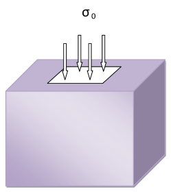
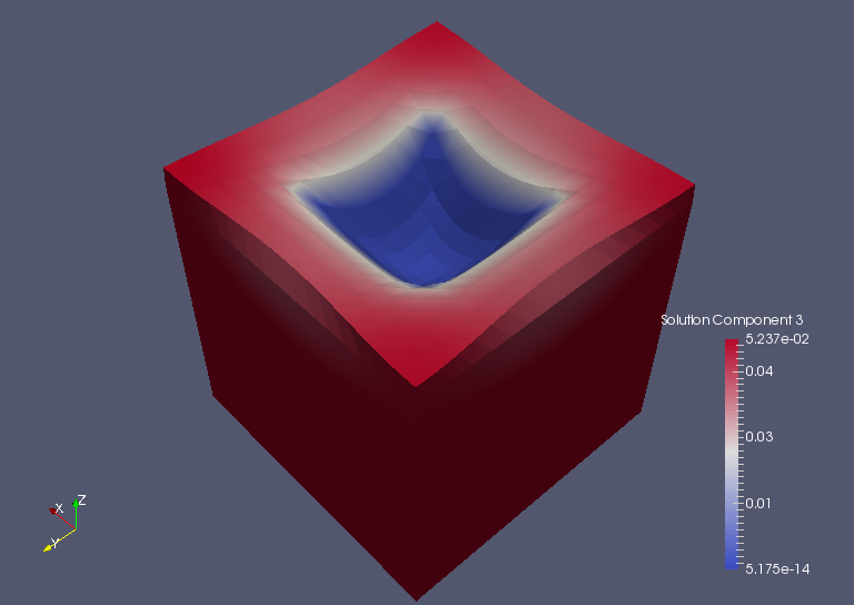
Figure 1: Computational domain and boundary conditions

We first study the performance of the preconditioners with respect to the mesh size $h$ and time step size $\tau$. Therefore, we fix $K=10^{-6}\,m^{2}$ and $\nu=0.2$. We use flexible GMRES as the outer iteration with a relative residual stopping criteria of $10^{-6}$. For $\mathcal{M}_{D}$, $\mathcal{M}_{L}$, and $\mathcal{M}_{U}$, the diagonal blocks are solved inexactly by preconditioned GMRES with a tolerance of $10^{-2}$. The results are shown in Figure 1. We see that the block preconditioners are effective and robust with respect to the discretization parameters $h$ and $\tau$.

Table 1: Iteration counts for the block preconditioners ($*$ means the direct method for solving diagonal blocks is out of memory)

	$\mathcal{B}_{D}$
	$\frac{1}{4}$	$\frac{1}{8}$	$\frac{1}{16}$	$\frac{1}{32}$
$0.1$	7	7	8	*
$0.01$	7	7	8	*
$0.001$	7	7	8	*
$0.0001$	7	7	8	*

$\mathcal{B}_{L}$
$\frac{1}{4}$	$\frac{1}{8}$	$\frac{1}{16}$	$\frac{1}{32}$
5	5	6	*
5	5	6	*
5	5	6	*
5	5	6	*

$\mathcal{B}_{U}$
$\frac{1}{4}$	$\frac{1}{8}$	$\frac{1}{16}$	$\frac{1}{32}$
4	4	4	*
4	4	5	*
5	5	6	*
5	5	6	*

$\mathcal{M}_{D}$
$\frac{1}{4}$	$\frac{1}{8}$	$\frac{1}{16}$	$\frac{1}{32}$
8	8	9	9
8	8	9	9
8	8	9	9
8	8	9	9

$\mathcal{M}_{L}$
$\frac{1}{4}$	$\frac{1}{8}$	$\frac{1}{16}$	$\frac{1}{32}$
6	6	8	8
6	6	8	8
6	6	8	8
7	6	8	8

$\mathcal{M}_{U}$
$\frac{1}{4}$	$\frac{1}{8}$	$\frac{1}{16}$	$\frac{1}{32}$
6	6	8	8
6	6	8	8
6	6	8	8
6	7	8	8

Next, we investigate the robustness of the block preconditioners with respect to the physical parameters $K$ and $\nu$. We fix the mesh size $h=1/16$ and time step size $\tau=0.01$. The results are shown Table 2. From the iteration counts, we can see that the proposed preconditioners are quite robust respect to the physical parameters.

Table 2: Iteration counts when varying $K$ or $\nu$

	$\nu=0.2$ and varying $K$
	$1$	$10^{-2}$	$10^{-4}$	$10^{-6}$	$10^{-8}$	$10^{-10}$
$\mathcal{B}_{D}$	4	7	8	8	8	8
$\mathcal{B}_{L}$	2	5	6	6	6	6
$\mathcal{B}_{U}$	3	4	5	5	5	5
$\mathcal{M}_{D}$	5	8	9	9	9	9
$\mathcal{M}_{L}$	5	7	8	8	8	8
$\mathcal{M}_{U}$	5	7	8	8	9	8

$K=10^{-6}$ and varying $\nu$
$0.1$	$0.2$	$0.4$	$0.45$	$0.49$	$0.499$
7	8	11	11	12	12
5	6	8	8	8	9
4	5	6	6	5	4
8	9	12	13	14	13
7	8	11	11	12	12
7	8	7	8	17	11

5 Conclusions

We have shown that the stability of the discrete problem, using stabilized finite elements, provides the means for designing robust preconditioners for the two-field formulation of Biot’s consolidation model. Our analysis shows uniformly bounded condition numbers and uniform convergence rates of the Krylov subspace methods for the preconditioned linear systems. More precisely, we prove that the convergence is independent of mesh size, time step, and the physical parameters of the model.

Current work includes extending this to non-conforming (and conforming) three-field formulations as in Hu.X;Rodrigo.C;Gaspar.F;Zikatanov.L2016a . For discretizations that are stable independent of the physical parameters, uniform block diagonal preconditioners can be designed using the framework developed here. Block lower and upper triangular preconditioners for GMRES can also be constructed in a similar fashion. In addition to their excellent convergence properties, the triangular preconditioners naturally provide an (inexact) fixed-stress split scheme for the three-field formulation.

References

• [1] James H. Adler, Xiaozhe Hu, and Ludmil T. Zikatanov. HAZMATH: A simple finite element, graph, and solver library.
• [2] James H Adler, Xiaozhe Hu, and Ludmil T Zikatanov. Robust solvers for Maxwell’s equations with dissipative boundary conditions. SIAM J. Sci. Comput., to appear.
• [3] G. Aguilar, F. Gaspar, F. Lisbona, and C. Rodrigo. Numerical stabilization of Biot’s consolidation model by a perturbation on the flow equation. Internat. J. Numer. Methods Engrg., 75(11):1282–1300, 2008.
• [4] T. Almani, K. Kumar, A. Dogru, G. Singh, and M.F. Wheeler. Convergence analysis of multirate fixed-stress split iterative schemes for coupling flow with geomechanics. Comput. Methods Appl. Mech. Engrg., 311(1):180 – 207, 2016.
• [5] Trygve Baerland, Jeonghun J Lee, Kent-Andre Mardal, and Ragnar Winther. Weakly imposed symmetry and robust preconditioners for biot’s consolidation model. arXiv preprint arXiv:1703.07792, 2017.
• [6] M. Bause, F.A. Radu, and U. Kocher. Space-time finite element approximation of the Biot poroelasticity system with iterative coupling. Computer Methods in Applied Mechanics and Engineering, 320:745 – 768, 2017.
• [7] L. Bergamaschi, M. Ferronato, and G. Gambolati. Block-partitioned solvers for coupled poromechanics: A unified framework. Comput. Methods Appl. Mech. Engrg., 196:2647 – 2656, 2007.
• [8] Maurice A. Biot. General theory of three‐dimensional consolidation. Journal of Applied Physics, 12(2):155–164, 1941.
• [9] Jakub Wiktor Both, Manuel Borregales, Jan Martin Nordbotten, Kundan Kumar, and Florin Adrian Radu. Robust fixed stress splitting for Biot’s equations in heterogeneous media. Applied Mathematics Letters, 68:101 – 108, 2017.
• [10] N. Castelleto, J. A. White, and M. Ferronato. Scalable algorithms for three-field mixed finite element coupled poromechanics. Journal of Computational Physics, 327:894 – 918, 2016.
• [11] N. Castelleto, J. A. White, and H. A. Tchelepi. Accuracy and convergence properties of the fixed-stress iterative solution of two-way coupled poromechanics. Int. J. Numer. Anal. Meth. Geomech., 39:1593 – 1618, 2015.
• [12] Stanley C Eisenstat, Howard C Elman, and Martin H Schultz. Variational iterative methods for nonsymmetric systems of linear equations. SIAM Journal on Numerical Analysis, 20(2):345–357, 1983.
• [13] Howard C Elman. Iterative methods for large, sparse, nonsymmetric systems of linear equations. PhD thesis, Yale University New Haven, Conn, 1982.
• [14] M. Ferronato, L. Bergamaschi, , and G. Gambolati. Performance and robustness of block constraint preconditioners in finite element coupled consolidation problems. Int. J. Numer. Meth. Engng, 81:381 – 402, 2010.
• [15] F. J. Gaspar, J. L. Gracia, F. J. Lisbona, and C. W. Oosterlee. Distributive smoothers in multigrid for problems with dominating grad-div operators. Numer. Linear Algebra Appl., 15(8):661–683, 2008.
• [16] F. J. Gaspar, F. J. Lisbona, C.W. Oosterlee, and R. Wienands. A systematic comparison of coupled and distributivesmoothing in multigrid for the poroelasticity system. Numer Linear Algebra Appl, 11:93–113, 2004.
• [17] Francisco J. Gaspar and Carmen Rodrigo. On the fixed-stress split scheme as smoother in multigrid methods for coupling flow and geomechanics. Submitted, 2017.
• [18] A. Greenbaum. Iterative Methods for Solving Linear Systems. SIAM, 1997.
• [19] Xiaozhe Hu, Carmen Rodrigo, Francisco J Gaspar, and Ludmil T Zikatanov. A nonconforming finite element method for the Biot’s consolidation model in poroelasticity. Journal of Computational and Applied Mathematics, 310:143–154, 2017.
• [20] J. Kim. Sequential methods for coupled geomechanics and multiphase flow. Stanford University, 2010.
• [21] J Kim, HA Tchelepi, and R Juanes. Stability and convergence of sequential methods for coupled flow and geomechanics: Fixed-stress and fixed-strain splits. Computer Methods in Applied Mechanics and Engineering, 200(13):1591–1606, 2011.
• [22] Jihoon Kim, Hamdi A Tchelepi, Ruben Juanes, et al. Stability, accuracy and efficiency of sequential methods for coupled flow and geomechanics. In SPE reservoir simulation symposium. Society of Petroleum Engineers, 2009.
• [23] Jeonghun J Lee, Kent-Andre Mardal, and Ragnar Winther. Parameter-robust discretization and preconditioning of biot’s consolidation model. SIAM Journal on Scientific Computing, 39(1):A1–A24, 2017.
• [24] D. Loghin and A. J. Wathen. Analysis of preconditioners for saddle-point problems. SIAM J. Sci. Comput., 25(6):2029–2049 (electronic), 2004.
• [25] P. Luo, C. Rodrigo, F. J. Gaspar, and C.W. Oosterlee. On an Uzawa smoother in multigrid for poroelasticity equations. Numer Linear Algebra Appl, page e2074.doi:10.1002/nla.2074, 2017.
• [26] Yicong Ma, Kaibo Hu, Xiaozhe Hu, and Jinchao Xu. Robust preconditioners for incompressible MHD models. Journal of Computational Physics, 316:721–746, 2016.
• [27] K.A. Mardal and R. Winther. Preconditioning discretizations of systems of partial differential equations. Numerical Linear Algebra with Applications, 2010.
• [28] Andro Mikelić and Mary F Wheeler. Convergence of iterative coupling for coupled flow and geomechanics. Computational Geosciences, 17(3):455–461, 2013.
• [29] C Rodrigo, FJ Gaspar, Xiaozhe Hu, and LT Zikatanov. Stability and monotonicity for some discretizations of the Biot’s consolidation model. Computer Methods in Applied Mechanics and Engineering, 298:183–204, 2016.
• [30] Joshua A White, Nicola Castelletto, and Hamdi A Tchelepi. Block-partitioned solvers for coupled poromechanics: A unified framework. Computer Methods in Applied Mechanics and Engineering, 303:55–74, 2016.