Grand-canonical Monte-Carlo simulation of solutions of salt mixtures: theory and implementation

Abstract

A Grand-canonical Monte-Carlo simulation method extended to simulate a mixture of salts is presented. Due to charge neutrality requirement of electrolyte solutions, ions must be added to or removed from the system in groups. This leads to some complications compared to regular Grand Canonical simulation. Here, a recipe for simulation of electrolyte solution of salt mixture is presented. It is then implemented to simulate solution of 1:1, 2:1 and 2:2 salts or their mixtures at different concentrations using the primitive ion model. The osmotic pressures of the electrolyte solutions are calculated and shown to depend linearly on the salt concentrations within the concentration range simulated. We also show that at the same concentration of divalent anions, the presence of divalent cations make it easier to insert monovalent cations into the system. This can explain some quantitative differences observed in experiments of the MgCl₂ salt mixture and MgSO₄ salt mixture.

I Introduction

Computer simulation is an integral part of many areas of modern interdisciplinary research in physics, chemistry, biology and material science Allen and Tildesley (1987). This is especially true for computer simulation of biological systems in medicine such as drug design and bioinspired novel materials and nanotechnology for medicine Coveney (2014). For such systems, molecular dynamics has been an important computational tool to understand physical characteristics of ligand-receptor binding processes, and to predict structural, dynamical and thermodynamic properties of biological molecules. However, although computing hardware has been steadily improved over the year, the large amount of atoms (correspondingly, the number of degrees of freedoms) in such system has rendered traditional molecular dynamics simulation to limited applications within few hundred nanoseconds and tens of nanometer scales. This computing requirement is even more demanding and challenging when the physics phenomenon involved require quantum mechanical simulation. To overcome such limitation and to bridge to larger time and spatial scales, multi-scale simulation strategies have been an active research. Among them, methods of hybrid Quantum mechanics/Molecular mechanics or Coarse-grained/Molecular Mechanics simulation, or Adaptive resolution simulation have been proposed with limited successPraprotnik and Site (2013); Potestio et al. (2013); Neri et al. (2005); Noid (2013); Brunk and Rothlisberger (2015).

The general idea behind multiscale simulation is to focus in molecular details to only a small, well-defined region (MM region) of interest while the rest of the system can be simulated at a coarser scale, making the computation more efficient. The bridging of macromolecules (such as protein or DNA) between two different scaled regions can be handled adequately in such hybrid simulation with suitable choice of coarse-grained model such as the Gō model Ueda et al. (1978); Hoang and Cieplak (2000) for protein or similar coarse-grained model for DNA Villa et al. (2005). This multiscale strategy also helps to avoid unnecessary bias due to potentially wrong orientations of the side chains far from the binding site. However, the simulation of mobile molecules, especially mobile ions, into and out of the MM region is still an open question which is not trivial to handle in a molecular dynamic simulation. In fact, one usually forbids the mobile ions to move in and out of the MM region in such simulation. One idea to overcome this is to look beyond molecular dynamics. Specifically, in addition to molecular dynamics simulation, one could try to implement a Monte-Carlo simulation in the Grand canonical ensemble. In such simulation, mobile ions could be inserted and removed from the MM region in such a way that their chemical potentials are fixed, and controlled by coupling to a particle reservoir with the correct concentration. This is actually desirable because all biological systems function in equilibrium with water solutions at given pH and salinity. Of course, developing and implementing such scheme for application in computational biomedicine or pharmaceutical nanotechnology require large amount of time and resources and it is a very active research area.

In this paper, as a first step in such direction, we present a Grand canonical Monte-Carlo (GCMC) simulation of electrolyte solutions for different salinity expanding upon a preliminary study of single salt electrolyte solution Valleau and Cohen (1980). We generalize them to different salt mixtures and present a detailed implementation of 1:1, 2:1, and 2:2 salt solutions and their mixture (such as both divalent and monovalent anions and cations are present). The fugacities of various type of salts in different solution and their osmotic pressure are studied. Additionally, the effect of additional salts on the fugacity of a given salt is studied. Our results show that, in asymmetric salt mixture, divalent cations can make it easier to insert monovalent cations into the solution.

The Grand-Canonical Monte-Carlo method was developed and used in several recent papers in our group to study the condensation of DNA inside bacteriophages in the presence of mixture of different salts, MgSO₄, MgCl₂, NaCl Lee et al. (2010); Nguyen (2013, 2016); Nguyen et al. (2017). However, detail of the method was never presented, only the simulation results of DNA system were shown. In this paper, the methodology and implementation of this GCMC method generalized for salt mixture is presented systematically and in detail. This allows for extension to any systems, not just DNA systems, and for potential integration in various multiscale simulation schemes.

The paper is organized as follows. In Sec. II, the Grand-canonical Monte-Carlo is formulated to simulate a system of salts mixture. In Sec. III, the detail implementation of this method for various salts and salt mixtures are presented. Result for the fugacities and osmotic pressure are reported and discussed. We conclude in Sec. IV.

II Grand canonical Monte$-$Carlo Simulation of electrolyte solutions : theoretical aspect

In a Grand Canonical Monte-Carlo (GCMC) simulation, the number of ions is not constant during the simulation. Instead their chemical potentials are fixed. To show how this is done, let us consider a state $i$ of the system that is characterized by the locations of $N_{iZ+}$ multivalent counterions, $N_{i+}$ monovalent counterions, $N_{iZ-}$ multivalent counterions, $N_{i-}$ coions (in the next section where we focus on divalent counterions and coions, $Z=2$). In the grand canonical ensemble of unlabeled particles, the probability of such state is given by

$$\pi_{i} = \frac{1}{\cal Z}\frac{1}{\Lambda_{Z+}^{3N_{iZ+}}\Lambda_{+}^{3N_{i+}}\Lambda_{Z-}^{3N_{iZ-}}\Lambda_{-}^{3N_{i-}}}$$ (1)

$$\quad\exp\left[\beta(\mu_{Z+}N_{iZ+}+\mu_{+}N_{i+}+\mu_{-}N_{i-}+\mu_{Z-}N_{iZ-}-U_{i}\right]$$

Here, $\cal Z$ is the grand canonical partition function, $\beta=1/k_{B}T$, $\Lambda_{x}\equiv h/\sqrt{2\pi m_{x}k_{B}T}$ are the thermal wavelength of the corresponding ion type (here $x$ are either $Z+,\ Z-,\ -$ or $+$), $U_{i}$ is the interaction energy of the state $i$, and $\mu_{x}$ are the corresponding chemical potential of the ions.

In a standard Monte Carlo simulation, one would like to generate a Markov chain of system states $i$ with a limiting probability distribution proportional to $\pi_{i}$. To do this, given a state $i$, one tries to move to state $j$ with probability $p_{ij}$. A sufficient condition for the Markov chain to have the correct limiting distribution is:

$$\frac{p_{ij}}{p_{ji}}=\frac{\pi_{i}}{\pi_{j}}$$ (2)

As usual, at each step of the chain, a “trial” move to change the system from state $i$ to state $j$ is attempted with probability $q_{ij}$ and is accepted with probability $f_{ij}$. Clearly,

$$p_{ij}=q_{ij}f_{ij}$$ (3)

It is convenient to regard the simulation box as consisting of $V$ discrete sites ($V$ is very large). Then for a trial move where $\nu_{\alpha}$ particles of species $\alpha$ are added to the system:

$$q_{ij}=\frac{1}{V^{\nu_{\alpha}}\nu_{\alpha}!}$$ (4)

Conversely, if $\nu_{\alpha}$ particles of species $\alpha$ are removed from the system:

$$q_{ij}=\frac{(N_{\alpha}-\nu_{\alpha})!}{N_{\alpha}!\nu_{\alpha}!}$$ (5)

Putting everything together, equations (1)$-$(5) give us a recipe to calculate the Metropolis acceptance probability of a particle insertion/deletion move in GCMC simulation. For example, if in a transition from state $i$ to state $j$, a multivalent salt molecule (one $Z-$ion and $Z$ coions) is added to the system, the Metropolis probability of acceptance of such move can be chosen as:

$$f_{M}=\min\{1,~{}f_{ij}/f_{ji}\}$$ (6)

where

$$\frac{f_{ij}}{f_{ji}}=\frac{B_{Z:1}}{(N_{iZ+}+1)(N_{i-}+1)...(N_{i-}+Z)}\exp[\beta(U_{i}-U_{j})],$$ (7)

with

$$B_{Z:1}=\exp(\beta\mu_{Z:1})\frac{V^{Z+1}}{\Lambda_{Z+}^{3}\Lambda_{-}^{3Z}},$$ (8)

and $\mu_{Z:1}=\mu_{Z+}+Z\mu_{-}$ is the combined chemical potential of a $Z:1$ salt molecule. On the other hand, if a multivalent salt molecule (one $Z-$ion and $Z$ coions) is removed from the system, we have:

$$\frac{f_{ij}}{f_{ji}}=\frac{N_{iZ+}N_{i-}...(N_{i-}-Z+1)}{B_{Z:1}}\exp[\beta(U_{i}-U_{j})],$$ (9)

Similar expressions are easily obtained from addition/removal of $Z:Z$ salt. For addition,

$$\frac{f_{ij}}{f_{ji}}=\frac{B_{Z:Z}}{(N_{iZ+}+1)(N_{iZ-}+1)}\exp[\beta(U_{i}-U_{j})],$$ (10)

and for removal,

$$\frac{f_{ij}}{f_{ji}}=\frac{N_{iZ+}N_{iZ-}}{B_{Z:Z}}\exp[\beta(U_{i}-U_{j})],$$ (11)

where

$$B_{Z:Z} = \exp(\beta\mu_{Z:Z})\frac{V^{2}}{\Lambda_{Z+}^{3}\Lambda_{Z-}^{3}}.$$ (12)

and $\mu_{Z:Z}=\mu_{Z+}+\mu_{Z-}$ is the combined chemical potential of $Z:Z$ salt molecule.

For the addition of monovalent $1:1$ salt to the system

$$\frac{f_{ij}}{f_{ji}}=\frac{B_{1:1}}{(N_{i+}+1)(N_{i-}+1)}\exp[\beta(U_{i}-U_{j})],$$ (13)

and for removal of $1:1$ salt,

$$\frac{f_{ij}}{f_{ji}}=\frac{N_{i+}N_{i-}}{B_{1:1}}\exp[\beta(U_{i}-U_{j})],$$ (14)

where

$$B_{1:1} = \exp(\beta\mu_{1:1})\frac{V^{2}}{\Lambda_{+}^{3}\Lambda_{-}^{3}},$$ (15)

and $\mu_{1:1}=\mu_{+}+\mu_{-}$ is the combined chemical potential of $1:1$ salt molecule.

Because we are trying to simulate a mixture of salts, to improve the system relaxation and to improve the sampling of the system’s phase space, in addition to adding/removing of salt molecules, one could add mixed Monte Carlo moves by both removing and adding ions of different species in a single step, so long as to maintain the charge neutrality. Most simple MC moves that one can add in the simulation is following: (a) one $Z+$ multivalent anion is added to (or removed from) the system and $Z$ monovalent anions are removed from (or added to) the system; (b) one $Z-$ multivalent cation is added to (or removed from) the system and $Z$ monovalent cations are removed from (or added to) the system. The acceptance probabilities of such moves are also easily calculated in the same manner. For example, if one $Z+$ anions is added to the system and $Z$ monovalent anions are removed the system, the Metropolis acceptance ratio is:

$$\frac{f_{ij}}{f_{ji}}=\frac{B_{1:1}^{Z}N_{i+}...(N_{i+}-Z+1)}{B_{Z:1}(N_{iZ+}+1)}\exp[\beta(U_{i}-U_{j})],$$ (16)

Vice versa, for a “trial” Monte-Carlo move where one $Z-$ cation is removed from the system and $Z$ monovalent cation are added to the system, the Metropolis acceptance ratio is:

$$\frac{f_{ij}}{f_{ji}}=\frac{B_{Z:1}N_{iZ+}}{B_{1:1}^{Z}(N_{i+}+1)...(N_{i+}+Z)}\exp[\beta(U_{i}-U_{j})].$$ (17)

Note that, in all the Metropolis acceptance above, one only needs 3 chemical potentials for the combined salts $\mu_{Z:1}$, $\mu_{Z:Z}$, and $\mu_{1:1}$, instead of four chemical potentials for individual ion species, $\mu_{x}$. This is because the system must maintain charge neutrality in all addition/deletion moves so all four chemical potentials are not independent. In our actual implementation, the scaled fugacities $B_{Z:1}$, $B_{Z:Z}$ and $B_{1:1}$, are used instead of the chemical potentials.

Beside particle addition/deletion moves, one also tries standard particle translation moves. They are carried out exactly like in the case of a canonical Monte-Carlo simulation. In a “trial” move from state $i$ to state $j$, an ion is chosen at random and is moved to a random position in a volume element surrounding its original position. The standard Metropolis probability is used for the acceptance of such “trial” move:

$$f_{M}=\min\{1,~{}\exp[\beta(U_{i}-U_{j})]\}.$$ (18)

III Grand canonical Monte$-$Carlo Simulation of electrolyte solution: implementation for different salt mixtures

In this section, the application of the grand$-$canonical Monte$-$Carlo simulation detailed in previous section to simulate a bulk concentration of electrolyte mixtures is presented. We will focus on the cases of 1:1, 2:1 and 2:2 salt solution and their mixtures. For simplicity, all ions have radius of $\sigma_{x}=2$Å. The primitive ion model is used. The aquaous solution is modeled implicitly as a continous medium with dielectric constant, $\varepsilon$. The interaction between two ions $\alpha$ and $\beta$ with radii $\sigma_{\alpha,\beta}$ and charges $Q_{\alpha,\beta}$ is given by

$$U=\left\{\begin{array}[]{l l}\dfrac{Q_{\alpha}Q_{\beta}}{\varepsilon r_{\alpha\beta}}&\quad\mbox{if $r_{\alpha\beta}>\sigma_{\alpha}+\sigma_{\beta}$}\\ \infty&\quad\mbox{if $r_{\alpha\beta}<\sigma_{\alpha}+\sigma_{\beta}$}\\ \end{array}\right.$$ (19)

where $r_{\alpha\beta}=|\mathbf{r}_{\alpha}-\mathbf{r}_{\beta}|$ is the distance between the ions.

The simulation is carried out using the periodic boundary condition. The long-range electrostatic interactions between charges in neighboring cells are treated using the standard Ewald summation method Ewald (1921).

To be able to calculate the pressure of the system, the Expanded Ensemble method Lyubartsev and Nordenskiöld (1995); Guldbrand et al. (1986) is implemented. This method allows us to calculate the difference of the system free energies at different volumes by sampling these volumes simultaneously in a simulation run. By sampling two nearly equal volumes, $V$ and $V+\Delta V$, and calculate the free energy difference $\Delta\Omega$, we can calculate the total pressure of the system:

$$P(T,V,\{\mu_{x}\})=-\left.\frac{\partial\Omega(T,V,\{\mu_{x}\})}{\partial V}\right|_{T,\{\mu_{x}\}}\simeq-\frac{\Delta\Omega}{\Delta V}$$ (20)

The volume derivative are taken at constant values of all four chemical potentials, $\{\mu_{x}\}\equiv\{\mu_{Z+},\mu_{Z-},\mu_{+},\mu_{-}\}$.

For each simulation run, 100 million MC moves are carried out depending on the average number of ions in the system. To ensure thermalization, 10 million initial moves are discarded before doing statistical analysis of the result of the simulation. All simulations are done using the physics simulation library SimEngine develop by one of the author (TTN). This library use OpenCL and OpenMP extensions of the C programming language to distribute computational workloads on multi-core CPU and GPGPU to speed up the simulation time. Both molecular dynamics and Monte-Carlo simulation methods are supported. In this paper the Monte-Carlo module of the library is used.

III.1 Finite size effect

The first question one asks is the limit of application of this GCMC method. For large system where the fluctuation in the particle number is fractionally small, the simulation result should give the same statistical property of canonical system. However, for small system where the particle number fluctuation is large, one might question of validity of the proposed method. To investigate this finite size effect, we simulate a salt mixture at the same chemical potentials (resulting in the same expected salt concentrations), but with different volume dimensions. Specifically, the scaled fugacities are $B_{2:2}/V^{2}=2.05\times 10^{-10}\mbox{\AA}^{-2}$, $B_{2:1}/V^{3}=1.14\times 10^{-14}\mbox{\AA}^{-3}$ and $B_{1:1}/V^{2}=5.50\times 10^{-10}\mbox{\AA}^{-2}$. These values are chosen so that, the solution contains a mixture of three different salts, 2:2 salts, 2:1 salt and 1:1 salt with the corresponding desired concentrations of approximately 200mM, 10mM and 50mM (note that, the scaled fugacities $B_{m:n}$, eqs. (8), (12) and (15) must be scaled appropriately for different volumes). The simulation box is a cubic box with side length varying from 20Å to 120Å, corresponds to the average number of particle of divalent anions from 0.7 to about 215.6. In Figure 1, the resultant concentrations at a given chemical potential is plotted as function of simulation box lengths. Similarly, Table 1 shows the numerical values obtained from our simulation for the averaged concentrations, particle numbers and osmotic pressures as function of the simulation box lengths.

Box length (Å)	$c_{2:2}$(mM)	$c_{2:1}$(mM)	$c_{1:1}$(mM)	$N_{2+}$	$N_{1+}$	$P_{b}$ (atm)
120	$197.2\pm 12.6$	$10.0\pm 42.7$	$50.1\pm 6.8$	$215.60\pm 13.16$	$52.11\pm 7.11$	$8.66\pm 0.20$
100	$197.0\pm 16.7$	$9.9\pm 16.9$	$50.2\pm 8.9$	$124.64\pm 10.16$	$30.21\pm 5.37$	$8.59\pm 0.10$
80	$196.4\pm 23.6$	$10.1\pm 24.1$	$50.0\pm 12.5$	$63.67\pm 7.44$	$15.43\pm 3.84$	$8.73\pm 0.15$
60	$197.6\pm 37.2$	$10.1\pm 15.8$	$50.0\pm 19.2$	$27.00\pm 4.86$	$6.51\pm 2.50$	$8.55\pm 0.16$
40	$197.1\pm 68.5$	$9.9\pm 68.9$	$50.2\pm 35.3$	$7.98\pm 2.65$	$1.93\pm 1.36$	$8.76\pm 0.04$
30	$193.9\pm 104.7$	$9.5\pm 105.5$	$48.0\pm 54.9$	$3.31\pm 1.72$	$0.78\pm 0.89$	$8.53\pm 0.18$
20	$144.5\pm 175.6$	$3.3\pm 178.1$	$18.7\pm 70.4$	$0.71\pm 0.86$	$0.09\pm 0.34$	$3.84\pm 0.10$

Table 1: The result salt concentrations and osmotic pressure of the solution as function of the length of the cubic simulation box. The chemical potential are fixed to have the desired mixture of concentrations of 200mM, 10mM and 50mM for 2:2 salt, 2:1 salt and 1:1 salt correspondingly.

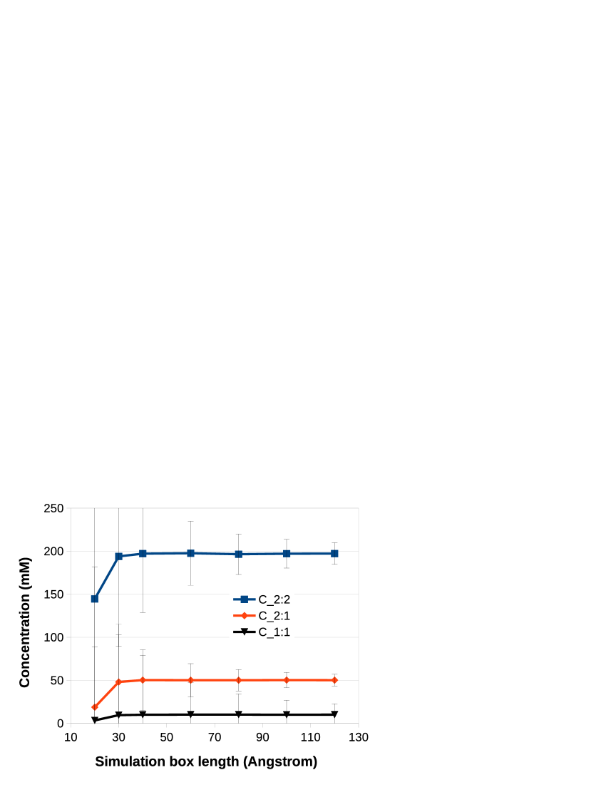
Figure 1: The concentrations of various component salt in a mixture of three different salts: 2:2, 2:1 and 1:1 salts. The chemical potentials of salt molecules are fixed. The size of the simulation box varies from 120Å down to 20Å. Size dependent effect is only observed for very small simulation volume such that, on average, there is less than one salt particle in the volume.

We can see that, within the uncertainty of the results, all concentrations are independent of simulation box length down to a very small box length. One only sees the finite size effect at simulation box length of about 30Å or smaller. At these small volumes, the average number of salt molecules in the simulation box is even smaller than one for some types (such as the number of $+1$ ions as shown in Table. 1 ). This suggests that as long as the simulation box are large enough to have a few ions in it on average, the grandcanonical Monte$-$Carlo method presented is reliable. For a given desired concentration, the chemical potential of the salts are independent on the sizes and shapes of the simulation box.

It should be mentioned here the obvious effect of reducing the simulation box size is the increase in the relative fluctuation in concentrations. This is inline with statistical theory which says that the particle number fluctuation increases as $\sqrt{N}$ with the number of particle, $N$. The columns 5 and 6 of Table 1 clearly show this quantitative trend. Because of this, the number fluctuation increases relatively as $1/\sqrt{N}$ as $N$ decreases. The error bar in Fig. 1 becomes very large at small simulation box size. Impressively, colume 5 and 6 of Table 1 show that the $\sqrt{N}$ estimate for fluctuation in the number of particles works even for the case the average number of ions is smaller than one.

In the rest of this paper, the simulation box volume is fixed $V=2.650\times 10^{3}\mbox{ nm}^{3}$, corresponding to a box length of 138.4Å, more than enough to eliminate possible finite size effects even at some small salt concentrations simulated.

III.2 Single salt solution

Let us present the result of our GCMC simulations for solution containing a single type of salt, either 1:1, 2:1 or 2:2 salt. Some concentrations simulated are already performed independently by the authors of Ref. Valleau and Cohen, 1980. For these concentrations, our results agree with their results. Thus, this section also serves as a check on the correctness of our code implementation.

Tables 2, 3, and 4 show the scaled fugacity $B$ and the resultant averaged concentration of the solution obtained from simulation using these parameters. Three different salts, $1:1$ salt, $2:1$ salt and $2:2$ salt are listed. Standard deviations in the concentration are about 10% in our simulation. This relative error is in line with those of previous GCMC simulations of Ref. Valleau and Cohen, 1980.

Additionally, the omotic pressure of the solution obtained from simulation is presented in column 3. These values are also plotted in Fig. 2 for easier comparison.

$B_{1:1}/V^{2}$ (Å-2)	$c$ (mM)	$P_{b}$ (atm)
$4.00\times 10^{-11}$	$11.7\pm 1.9$	$0.552\pm 0.003$
$1.15\times 10^{-10}$	$20.3\pm 2.6$	$0.954\pm 0.007$
$6.60\times 10^{-10}$	$51.99\pm 4.2$	$2.40\pm 0.012$
$2.30\times 10^{-9}$	$101.4\pm 5.7$	$4.683\pm 0.023$
$8.80\times 10^{-9}$	$206.2\pm 10.2$	$9.572\pm 0.001$

Table 2: The scaled fugacity, $B_{1:1}$ of the 1:1 salt at different concentrations. Columns 2 and 3 show the corresponding salt concentration and osmotic pressure of the salt bulk solution obtained from simulation.

$B_{2:1}/V^{3}$ (Å-3)	$c$ (mM)	$P_{b}$ (atm)
$3.22\times 10^{-16}$	$10.03\pm 1.56$	$0.066\pm 0.005$
$1.80\times 10^{-15}$	$19.60\pm 2.19$	$1.26\pm 0.008$
$1.90\times 10^{-14}$	$50.75\pm 3.69$	$3.16\pm 0.03$
$1.00\times 10^{-13}$	$100.80\pm 7.71$	$6.16\pm 0.05$
$8.90\times 10^{-13}$	$245.57\pm 9.63$	$15.03\pm 0.07$

Table 3: The scaled fugacity, $B_{2:1}$ of the 2:1 salt for different concentrations. Columns 2 and 3 show the corresponding salt concentration and osmotic pressure of the bulk salt solution obtained from simulation.

$B_{2:2}/V^{2}$ (Å-2)	$c$ (mM)	$P_{b}$ (atm)
$6.36\times 10^{-12}$	$10.03\pm 2.26$	$0.379\pm 0.003$
$1.50\times 10^{-11}$	$20.81\pm 3.07$	$0.709\pm 0.028$
$4.45\times 10^{-11}$	$50.56\pm 5.37$	$1.60\pm 0.016$
$9.70\times 10^{-11}$	$100.81\pm 7.29$	$2.96\pm 0.033$
$2.50\times 10^{-10}$	$241.39\pm 14.68$	$6.82\pm 0.130$

Table 4: The scaled fugacity, $B_{2:2}$ of the 2:2 salt for different salt concentrations. Columns 2 and 3 show the corresponding salt concentration and osmotic pressure of the bulk salt solution obtained from simulation.

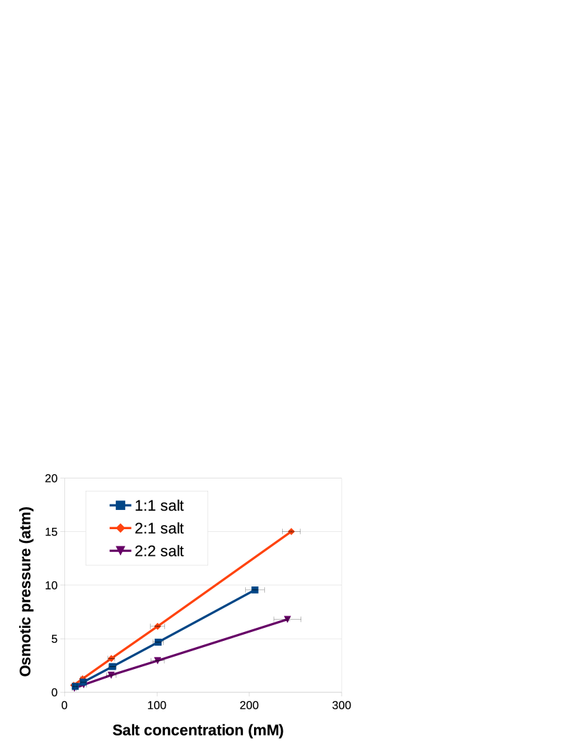
Figure 2: The osmotic pressure of the electrolyte solution containing a single type of salt. The pressure increases linearly with concentration within the range studied.

As one can see, at the same concentration, the osmotic pressure of 2:2 salt solution is lowest, while that of 2:1 salt is highest. This behaviour can be understood. Figure 2 shows that, for the concentration range studied, the osmotic pressure increases linearly with concentration. At these low concentrations, our solution should follow the van der Waals equation of stateLandau and Lifshitz (2013):

$$\left(P+\frac{n^{2}a}{V^{2}}\right)(V-nb)=nRT,$$ (21)

where $n$ is the number of moles of the particles and $a$, and $b$ are the pressure and volume corrections due to non-ideality. The volume correction parameter, $b$, of this equation is small for our system. However, the pressure correction parameter, $a$, of the van der Waals equation of state depends on interactions among different ions. This is why, at the same concentration, both 1:1 salt and 2:2 salt contain the same number of ions but the pressure of 2:2 salt solution is lower due to much stronger attraction among cations and anions. On the other hand, for 2:1 salt, there are 3 ions dissolved per molecule compared to 2 ions dissolved for the other two salts. As a result, the number of moles of particles are 1.5 times higher than other solution, $n_{2:1}=1.5n_{1:1}$, leading to higher pressure.

III.3 Mixture of two salts

Next steps, we demonstrate the application of our general GCMC method to simulate the system of two salts, 1:1 salt and 2:1 salt. In a typical physiological experimental setup with 2:1 divallent salt, one usually has a buffer solution containing 50mM monovalent salt to maintain pH of the solution. Therefore, in the simulation, we simulate a solution mixture of 50mM 1:1 salt with varying 2:1 salt concentration.

$B_{2:1}/V^{3}$ (Å${}^{-3})$	$B_{1:1}/V^{2}$ (Å${}^{-2})$	$c_{2:1}$ (mM)	$c_{1:1}$ (mM)	$P_{b}$ (atm)
$4.00\times 10^{-15}$	$8.71\times 10^{-10}$	$13.9\pm 3.2$	$50.0\pm 5.9$	$3.18\pm 0.001$
$1.38\times 10^{-14}$	$1.15\times 10^{-9}$	$29.9\pm 3.5$	$50.2\pm 5.0$	$4.17\pm 0.001$
$7.78\times 10^{-14}$	$1.86\times 10^{-9}$	$74.7\pm 5.1$	$50.2\pm 5.3$	$6.87\pm 0.003$
$1.42\times 10^{-13}$	$2.25\times 10^{-9}$	$99.8\pm 5.7$	$50.3\pm 5.4$	$8.39\pm 0.006$
$3.45\times 10^{-13}$	$3.03\times 10^{-9}$	$150.2\pm 8.4$	$50.6\pm 6.7$	$11.4\pm 0.02$
$1.74\times 10^{-12}$	$5.29\times 10^{-9}$	$299.6\pm 11.2$	$49.4\pm 6.8$	$20.8\pm 0.04$

Table 5: The scaled fugacities $B_{2:1}$ and $B_{1:1}$ of 1:1 and 2:1 two-salt mixture. Columns 3 and 4 show the corresponding salt concentrations of the simulated bulk solution, the 1:1 salt concentration is kept approximately constant at 50mM. Column 5 shows the osmotic pressure of the bulk solution.

In columns 3 and 4 of table 5, the resultant salt concentrations, $c_{2:1}$ and $c_{1:1}$, of the bulk solution obtained from simulations are listed. The divalent salt concentration is varied from 10 mM to 300 mM while the monovalent salt concentration is kept at approximately 50 mM. Note that, even though $c_{1:1}$ is kept constant, $B_{1:1}$, (and correspondingly the monovalent salt chemical potential $\mu_{1:1}$) is not a constant but actually increases with $c_{2:1}$, being smallest at $c_{2:1}=0$. This is expected because in the system simulated here we use the same type of monovalent cation for both salts. Increasing 2:1 salt concentration leads to an increase in the accompanied concentration of the $-1$ cations. As a result, the chemical potential of 1:1 salt (which is the sum of the chemical potentials of both $+1$ anions and $-1$ cations) increases. The linear dependence of the fugacity $B_{1:1}$ on $c_{2:1}$ shown in Fig. 3 agrees with this argument.

III.4 Mixture of three different salts

$B_{2:2}/V^{2}$ (Å${}^{-2})$	$B_{2:1}/V^{3}$ (Å${}^{-3})$	$B_{1:1}/V^{2}$ (Å${}^{-2})$	$c_{2:2}$ (mM)	$c_{2:1}$ (mM)	$c_{1:1}$ (mM)	$P_{b}$ (atm)
$5.86\times 10^{-12}$	$3.86\times 10^{-15}$	$7.58\times 10^{-10}$	$9.9\pm 3.0$	$10.1\pm 3.9$	$49.9\pm 6.2$	$3.26\pm 0.04$
$1.36\times 10^{-11}$	$4.70\times 10^{-15}$	$7.15\times 10^{-10}$	$20.2\pm 4.3$	$9.8\pm 4.9$	$49.8\pm 6.4$	$3.54\pm 0.03$
$4.13\times 10^{-11}$	$6.74\times 10^{-15}$	$6.63\times 10^{-10}$	$49.9\pm 6.7$	$10.1\pm 7.0$	$49.9\pm 6.5$	$4.40\pm 0.01$
$9.45\times 10^{-11}$	$8.75\times 10^{-15}$	$6.02\times 10^{-10}$	$99.7\pm 9.3$	$9.9\pm 9.5$	$50.0\pm 6.7$	$5.86\pm 0.02$
$1.50\times 10^{-10}$	$1.03\times 10^{-14}$	$5.71\times 10^{-10}$	$150.1\pm 11.4$	$10.2\pm 11.5$	$50.0\pm 6.8$	$7.25\pm 0.03$
$2.05\times 10^{-10}$	$1.14\times 10^{-14}$	$5.50\times 10^{-10}$	$200.0\pm 15.5$	$10.1\pm 15.5$	$50.2\pm 6.8$	$8.33\pm 0.30$
$3.30\times 10^{-10}$	$1.35\times 10^{-14}$	$5.22\times 10^{-10}$	$307.7\pm 15.0$	$9.9\pm 19.4$	$50.1\pm 6.8$	$11.4\pm 0.05$

Table 6: The scaled fugacities, $B_{2:2}$, $B_{2:1}$ and $B_{1:1}$, of the three salts in the mixture. Columns 4, 5 and 6 show the corresponding salt concentrations. The 1:1 salt concentration is kept approximately constant at 50mM. The 2:1 salt concentration is kept approximately constant at 10mM. Column 7 shows the osmotic pressure of the bulk solution obtained from simulation.

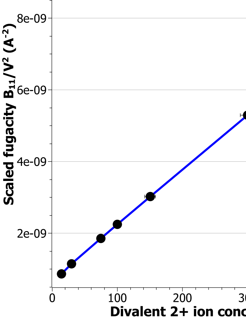
a)

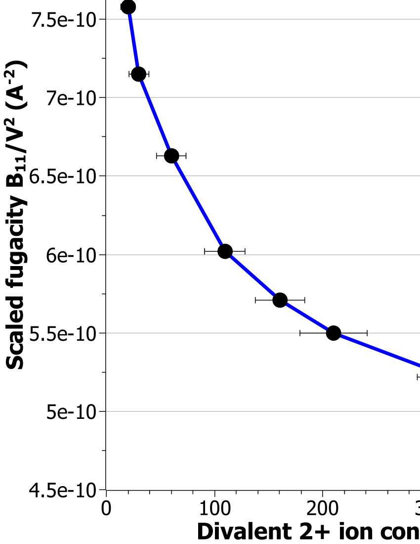
b)

Figure 3: The scaled fugacity $B_{11}$ of 1:1 monovalent salt as function of the divalent anion concentrations. It increases with increasing divalent anion concentrations for the case of no divalent cations (a); it decreases with increasing divalent anions in the presence of divalent cations (b). In both case, the simulated solution contains about 50mM monovalent salt. The opposite behaviors of $B_{11}$ shows that divalent cations make it easier to insert monovalent cations into solution (see text for more discussion).

Lastly, we report on the more complicated but experimentally relevant case of an electrolyte solution where all three 2:2, 2:1 and 1:1 salts are present. Such a mixture is used in studying the effect of MgSO₄ salt on DNA ejection from bacteriophages such as that done in Ref. Evilevitch et al. (2008). While the MgSO₄ salt (2:2 salt) concentration varies, the pH of the solution is maintained using a buffer solution of 10mM MgCl₂ and 50mM NaCl. Consequently, in this section, we report on simulation of solution containing varying concentration of 2:2 salt, while keeping the 1:1 salt concentration fixed at 50mM, and 2:1 salt concentration fixed at 10mM. The monovalent cations are assumed to be the same for both salts (Cl^-1 ions in experiments). Table 6 list the corresponding fugacity parameters $B$ of the three salts in solution. Similar to previous sections, the resultant concentrations of the ion species are reported in columns 4, 5 and 6. The osmotic pressure of the solution is reported in the last columns. A very important physical observation for this three salt mixture is the fact that, in the presence of divalent cations, the fugacity of monovalent salt decreases with increasing divalent anion concentrations. In other words, divalent cations make it easier to insert monovalent cations into the solution. This is show clearly in Fig. 3 where the scale fugacity $B_{11}$ is plotted for different divalent anion concentrations without (Fig. 3a) and with (Fig. 3b) the presence of divalent cations.

The opposite behaviors of $B_{11}$ shows that divalent cations make it easier to insert monovalent cations into solution. Physically, one could explain this behaviour by the fact that it takes one divalent cations instead of two monovalent cations to conpensate for the charges of divalent anions. Entropically, this leaves “room” in the system to add more monovalent salt to the solution. Experimentally, there is quantitative difference between DNA ejection from bacteriophages in MgCl₂+NaCl solution and MgSO₄+MgCl₂+NaCl solution Evilevitch et al. (2008). Our simulation showing monovalent salt can enter bacteriophages easier in the presence of MgSO₄ (2:2) salt qualitatively agrees with the experimental fact that that MgSO₄ make DNA ejection easier. Nevertheless, more detail investigation is needed. This will be studied in a future work.

Before conluding this section, let us show some preliminary result on the effect of ion sizes on the fugacities and the pressure of electrolyte solution. Mixture of 2:1 and 1:1 salts is studied with the 1:1 salt concentration approximately 50mM. The 2:1 salt concentration is varied from about 20mM to 500mM. The radius of the divalent cation is simulated at 2Å, 2.5Åand 3Å respectively.

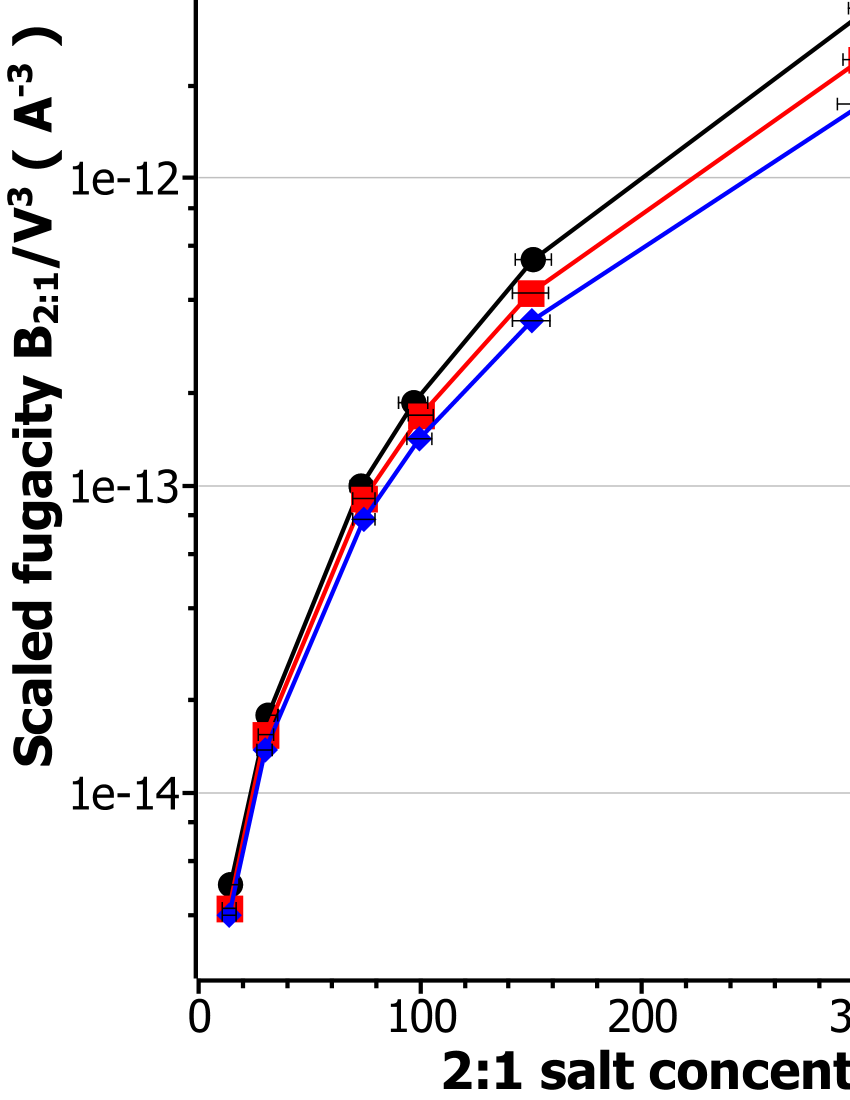
a)

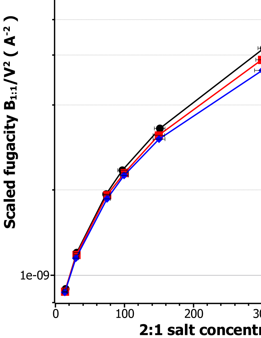
b)

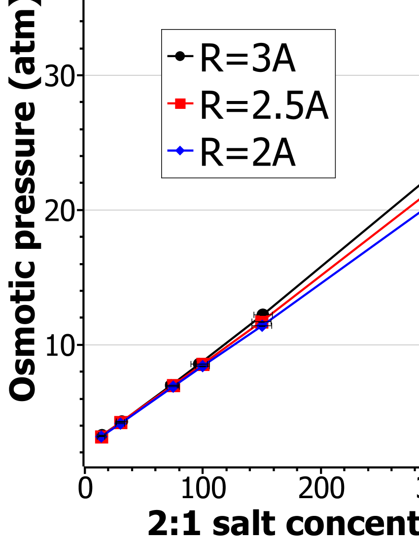
c)

Figure 4: The scaled fugacity $B_{11}$ of 1:1 monovalent salt (a) and $B_{21}$ of 2:1 divalent salt (b) and the osmotic pressure (c) in a mixture of the two salts as function of the divalent anion concentrations. Different curves corresponding to different value of the radius of the divalent anion, 2Å, 2.5Å, and 3Å. (see text for more discussion).

In Fig. 4, the fugacities of 2:1 salt and 1:1 salt in the mixture and the osmotic pressure is plotted. They show that increasing the size of $+2$ anions leads to increased fugacities and pressure at higher concentrations. This is inline with the van der Waals equation of state where the volume correction terms $b$ becomes larger for larger ions. Nevertheless, within the size range studied, this leads to about less than 10% corrections to the fugacity and pressure up to 500mM divalent salt concentration.

IV Conclusion

In this paper, we presented an extensive study of the Grand-Canonical Monte-Carlo simulation for electrolyte solutions using a primitive ion mode. Application of this method to simulate various solutions containing single salt, two salt mixture and three salt mixture are carried out. The fugacities of individual salt species for different solutions at typical concentrations are reported. The result of osmotic pressure of the electrolyte solution are calculated and shown to be linearly proportional to the salt concentration within the range of concentrations considered. However, the pressure differs for different type of salt because the non-ideal gas corrections are different for different ion valence.

Comparing the solution without and with divalent cations, it is shown that divalent cations make it easier to insert monovalent cations in solution. This agrees qualitatively with experimental result of DNA ejection from bacteriophages in MgSO₄ salt mixtures and MgCl₂ salt mixtures.

In this paper, the aqueous solution is simulated implicitly. It appears only in the dielectric constant of the medium. Our method is suitable therefore for a coarse-grained region in a multiscale simulation setup. If one simulates the solvent molecules explicitly, it is likely that a full particle insertion or deletion would be impractical due to a large change in the system energy. In such case, partial deletion/insertion of particle is preferable. Nevertheless, it is very unlikely one would practically need grand-canonical simulation in the atomistic region in a multiscale simulation.

V Acknowledgments

We would like to thank Drs. T. X. Hoang and Paolo Carloni for valuable discussions. TTN acknowledges the financial support of the Vietnam National University grant number QG.16.01 and, partially by the USA National Science Foundation grant NFS CBET-1134398. The authors are indebted to Dr A. Lyubartsev for providing us with the Fortran source code of their Expanded Ensemble Method.

References

- Allen and Tildesley (1987) M. P. Allen and D. J. Tildesley, Computer Simulation of Liquids (Clarendon Press, Oxford, 1987).
- Coveney (2014) P. Coveney, Computational biomedicine: modelling the human body (Oxford University Press, Oxford, 2014).
- Praprotnik and Site (2013) M. Praprotnik and L. D. Site, Biomolecular Simulations: Methods and Protocols , 567 (2013).
- Potestio et al. (2013) R. Potestio, S. Fritsch, P. Español, R. Delgado-Buscalioni, K. Kremer, R. Everaers, and D. Donadio, Phys. Rev. Lett. 110, 108301 (2013).
- Neri et al. (2005) M. Neri, C. Anselmi, M. Cascella, A. Maritan, and P. Carloni, Phys. Rev. Lett. 95, 218102 (2005).
- Noid (2013) W. Noid, J. Chem. Phys. 139, 090901 (2013).
- Brunk and Rothlisberger (2015) E. Brunk and U. Rothlisberger, Chemical reviews 115, 6217 (2015).
- Ueda et al. (1978) Y. Ueda, H. Taketomi, and N. Gō, Biopolymers 17, 1531 (1978).
- Hoang and Cieplak (2000) T. X. Hoang and M. Cieplak, J. Chem. Phys. 112, 6851 (2000).
- Villa et al. (2005) E. Villa, A. Balaeff, and K. Schulten, Proc. Nat. Acad. Science USA 102, 6783 (2005), http://www.pnas.org/content/102/19/6783.full.pdf .
- Valleau and Cohen (1980) J. P. Valleau and L. K. Cohen, J. Chem. Phys. 72, 5935 (1980).
- Lee et al. (2010) S. Lee, T. T. Le, and T. T. Nguyen, Phys. Rev. Lett. 105, 248101 (2010).
- Nguyen (2013) T. T. Nguyen, J. Biol. Phys. 39, 247 (2013).
- Nguyen (2016) T. T. Nguyen, J. Chem. Phys. 144, 065102 (2016).
- Nguyen et al. (2017) V. D. Nguyen, T. T. Nguyen, and P. Carloni, J. Biol. Phys. (2017), 10.1007/s10867-017-9443-x.
- Ewald (1921) P. P. Ewald, Ann. Phys. 64, 253 (1921).
- Lyubartsev and Nordenskiöld (1995) A. P. Lyubartsev and L. Nordenskiöld, J. Phys. Chem. 99, 10373 (1995).
- Guldbrand et al. (1986) L. Guldbrand, L. G. Nilsson, and L. Nordenskiöld, J. Chem. Phys. 85, 6686 (1986).
- Landau and Lifshitz (2013) L. Landau and E. Lifshitz, Statistical Physics, tập 5 (Elsevier Science, 2013).
- Evilevitch et al. (2008) A. Evilevitch, L. T. Fang, A. M. Yoffe, M. Castelnovo, D. C. Rau, V. A. Parsegian, W. M. Gelbart, and C. M. Knobler, Biophys. J. 94, 1110 (2008).