On-Shell Gauge Invariant Three-Point Amplitudes

Abstract

Assuming locality, Lorentz invariance and parity conservation we obtain a set of differential equations governing the 3-point interactions of massless bosons, which in turn determines the polynomial ring of these amplitudes. We derive all possible 3-point interactions for tensor fields with polarisations that have total symmetry and mixed symmetry under permutations of Lorentz indices. Constraints on the existence of gauge-invariant cubic vertices for totally symmetric fields are obtained in general spacetime dimensions and are compared with existing results obtained in the covariant and light-cone approaches.
Expressing our results in spinor helicity formalism we reproduce the perhaps mysterious mismatch between the covariant approach and the light cone approach in 4 dimensions. Our analysis also shows that there exists a mismatch, in the 3-point gauge invariant amplitudes corresponding to cubic self-interactions, between a scalar field $\phi$ and an antisymmetric rank-2 tensor field $A_{\mu\nu}$. Despite the well-known fact that in 4 dimensions rank-2 anti-symmetric fields are dual to scalar fields in free theories, such duality does not extend to interacting theories.

1 Introduction

The gauge principle has evolved over the past century from an insight of Weyl to being held as a guiding principle for constructing quantum theories that describe the interactions of elementary particles. The current paradigm of particle physics is summed up in the Standard Model (SM) with $SU(3)\times SU(2)\times U(1)$ gauge bosons interacting with the observed multiplets of quarks and leptons. While there are numerous attempts to extend this paradigm, the most noticeable being supersymmetry [1, 2], there are also efforts to extend the gauge interactions to higher spin fields [12, 13, 6, 20, 5, 16, 17, 18, 21, 19, 7, 23, 22]. The difficulty of constructing interacting theories involving only finitely many spins were already noticed in some of these early works [14]. The most recent attempts to extend the gauge sector to infinitely higher spins can be found in, e.g. [3, 4]; see also works in this directions from the string perspective [16, 17].

Since the 1980s there have been various approaches to determine the possible higher-spin interactions, the first attempts being by Bengtsson et al [12, 13] in which three-point higher-spin vertices, unique for a particular set of spins, were obtained in the light-cone formalism. A more general result was later obtained in [6] by a similar method, in which Metsaev used commutators of the Poincaré algebra to obtain the parity-even cubic vertices for massless fields in four dimensions, the cubic vertices for massless totally-symmetric fields in five dimensions and the cubic vertices for massless fields in six dimensions. The covariant approach was initiated in [14], as they constructed the unique self-interactions for massless spin-1, 2, 3 fields and interactions of two scalars with a spin-$s$ boson using the Fronsdal fields. This line of research was recently completed by Manvelyan et al. [15]. Sagnotti et al. [16] and Fotopoulos et al. [17] derived the same results from the string theory.

On the 3-point amplitudes Benincasa and Cachazo [5] exploited the technique of spinor helicity to derive a general form of helicity amplitudes for three massless particles. But this construction does not manifest the gauge symmetry, since spinors transform trivially under the translations (the gauge transformations in this case) in the little group. Therefore given a spinor helicity amplitude in [5] it is not clear whether there exists a Lagrangian description of a gauge theory which could lead to such an amplitude or not. It is, nevertheless, possible to include gauge transformations in the spinor helicity formalism (for example, see [11]). Benincasa and Cachazo used BCFW to investigate a class of “constructible” theories and found that there are no nontrivial amplitudes of different species of spin-2 particles or particles with spin larger than 2 among this class of theories, while a theory with a single kind of spin-2 particles is unique. Lately Boels and Medina [7] have obtained the three-point amplitudes using the constraints of on-shell gauge invariance. Their results are expressed in terms of polarization tensors with the gauge transformations manifest; these have been done for polarization vectors and rank-2 polarization tensors, but not for general polarizations.

There emerges a series of works combining these two approaches to study the spinor helicity amplitudes [19, 22, 23], the most notable discovery being a mismatch between the light-cone and covariant approaches: there are cubic vertices existing in light-cone approach but are absent in the covariant approach [19, 22, 23, 21]. As it turns out, the missing part is crucial for the existence of the higher-spin theory in 4d Minkowski spacetime, as pointed out by [19] and [23].

In this paper we study the 3-point gauge-invariant amplitudes which are expressed in terms of polarization tensors. Lorentz invariance and locality give strong constraints on the amplitudes in gauge theories so it is natural to use these constraints to select the possible theories. We focus on the parity conserved theories.

Let us first clarify what we mean by gauge invariance. We use the term gauge in the situation where the descriptions in a theory have redundancies. For example two polarization vectors $e_{\mu}(p)$ and $e_{\mu}(p)+p_{\mu}$ describe the same physical state of a massless spin-1 boson. This is a redundancy in the description. We use the term gauge invariance to refer to the fact that all physical quantities, such as scattering amplitudes, do not depend on how we describe a particular physical state. Although in the following discussion, we only consider the variation of the polarization tensors, our discussion is still valid for Non-Abelian Gauge theories: at the zeroth order (in coupling constant $g$) the gauge transformation does not change the color of the external states (the term containing $f^{abc}$ also has a factor $g$). Therefore we can simply drop the factor $f^{abc}$ in the following discussion on the gauge invariance of 3-point amplitudes.

With these theoretical assumptions we start with the 3-point gauge-invariant amplitudes of totally symmetric fields whose polarizations can be written as $\epsilon^{\pm}(p)=\bigotimes_{i=1}^{s}e^{\pm}(p)$. We find four basic gauge-invariant amplitudes, from which all possible the 3-point gauge-invariant amplitudes of three totally symmetric tensor fields can be constructed. We are able to give constraints on the total number of derivatives that are allowed to appear in a 3-point gauge-invariant vertex. Although we present our work in 3+1 dimensions, our analysis of the totally symmetric fields is valid for d+1 dimensions ($d\geq 3$): since changing the dimensions changes neither the form of polarization tensors nor their gauge transformations for totally symmetric tensor [20]. Whereas the number of polarization directions can change, the polarization tensors in this case are tensor products of polarization vectors in the same direction. One special thing, nevertheless, arises in four dimensions: many of the otherwise allowed amplitudes may vanish due to a Schouten-like identity.

The general results are summarized as follows,

$$A(\epsilon_{1},\epsilon_{2},\epsilon_{3};N)$$ (1.1)

$$= (e_{1}\cdot p_{2})^{\frac{s_{1}-s_{2}-s_{3}+N}{2}}(e_{2}\cdot p_{1})^{\frac{s_{2}-s_{1}-s_{3}+N}{2}}(e_{3}\cdot p_{1})^{\frac{s_{3}-s_{1}-s_{2}+N}{2}}A_{\text{YM}}(e_{1},e_{2},e_{3})^{\frac{s_{1}+s_{2}+s_{3}-N}{2}}$$

where $N$ is the total number of derivatives in the cubic vertex and

$$A_{\text{YM}}(e_{1},e_{2},e_{3})\equiv(e_{1}\cdot p_{2})(e_{2}\cdot e_{3})-(e_{2}\cdot p_{1})(e_{1}\cdot e_{3})+(e_{3}\cdot p_{1})(e_{1}\cdot e_{2})$$ (1.2)

In 4-dimension, however, due to a Schouten type identity, the non-trivial amplitudes are given by (assuming $s_{1}\leq s_{2}\leq s_{3}$ for convenience)

$$(e_{1}\cdot p_{2})^{s_{1}}(e_{2}\cdot p_{1})^{s_{2}}(e_{3}\cdot p_{1})^{s_{3}}～，$$ (1.3)

and

$$(e_{2}\cdot p_{1})^{s_{2}-s_{1}}(e_{3}\cdot p_{1})^{s_{3}-s_{1}}A_{YM}^{s_{1}}~{}.$$ (1.4)

Next we turn our attention to the 3-point gauge-invariant amplitudes of fields with mixed symmetries. We show that, like in the case of totally symmetric fields, there are certain basic amplitudes which can be used to construct all other amplitudes; we provide a detailed recipe to do so. It is known (for example, see [20]) that all massless mixed-symmetry fields are dual to totally-symmetric fields in the free theory in 4-dimension. Our result shows that this duality does not extend to the interacting theory: there exists a mismatch between the 3-point amplitudes upon introduction of interaction. Expressing our results in spinor helicity formalism we show that in two representations of the same helicity if the 3-point amplitudes for a given set of momenta do exist in both theories, these two amplitudes must be the same (up to coupling constants). This is because the 3-point amplitudes in spinor helicity formalism only depend on their helicities. Also in the spinor-helicity formalism, we can derive the conditions for non-vanishing amplitudes. This constraint is, however, missing in the light-cone approach. Therefore we can reproduce, and perhaps help to elucidate, the mismatch between the covariant approach and the light-cone approach.

The article is organized as follows: In the next section, we briefly review polarizations and gauge transformations to set notations. In Section 3 we discuss the gauge invariant 3-point amplitudes of higher-spin fields with total symmetry and mixed symmetry in their Lorentz indices. In Section 4 we present an example of how to construct a specific amplitude. And Section 5 is a brief conclusion and a short discussion. A straight forward derivation for all possible gauge invariant 3-point amplitudes in the case of totally-symmetric tensors is presented in Appendix.

2 Polarizations and Gauge Transformations

In the construction of a Hamiltonian with field operators that leads to a Lorentz invariant S-matrix, a generic field operator $\psi_{l}$ is required to transform according to a representation of the Lorentz group [8, 9]:

$$U(\Lambda,a)\psi_{l}(x)U^{-1}(\Lambda,a)=\sum_{l^{\prime}}D_{ll^{\prime}}(\Lambda^{-1})\psi_{l^{\prime}}(\Lambda x+a)$$ (2.1)

where $U(\Lambda,a)$ is the operator corresponding to the Poincaré transformation $x^{\prime}=\Lambda x+a$. In the case of a rank-$r$ tensor field $\phi^{\mu_{1}\cdots\mu_{r}}$ describing a massless spin $s$ particle, the condition (2.1) is fulfilled if the field operator is of the form

$$\phi^{\mu_{1}\cdots\mu_{r}}=\frac{1}{(2\pi)^{3/2}}\sum_{\sigma=\pm s}\int\frac{d^{3}p}{\sqrt{2p^{0}}}\left[\epsilon^{\mu_{1}\cdots\mu_{r}}(\mathbf{p},\sigma)a(\mathbf{p},\sigma)e^{ip\cdot x}+\epsilon^{\mu_{1}\cdots\mu_{r}}(\mathbf{p},\sigma)^{*}{a^{c}}^{\dagger}(\mathbf{p},\sigma)e^{-ip\cdot x}\right]$$ (2.2)

with the polarization tensor satisfying [8]

$${D\left[R(\theta)\right]^{\mu^{\prime}_{1}\cdots\mu^{\prime}_{r}}}_{\mu_{1}\cdots\mu_{r}}\epsilon^{\mu_{1}\cdots\mu_{r}}(\mathbf{k},\sigma)=\epsilon^{\mu^{\prime}_{1}\cdots\mu^{\prime}_{r}}(\mathbf{k},\sigma)e^{i\sigma\theta}\quad(\sigma=\pm s)$$ (2.3)

$${D\left[S(\alpha,\beta)\right]^{\mu^{\prime}_{1}\cdots\mu^{\prime}_{r}}}_{\mu_{1}\cdots\mu_{r}}\epsilon^{\mu_{1}\cdots\mu_{r}}(\mathbf{k},\sigma)=\epsilon^{\mu^{\prime}_{1}\cdots\mu^{\prime}_{r}}(\mathbf{k},\sigma)$$ (2.4)

where $k=(1,0,0,1)$ is a standard momentum and $R(\theta)$, $S(\alpha,\beta)$ are the little group transformations:

$${R(\theta)^{\mu}}_{\nu} =\begin{bmatrix}1&0&0&0\\ 0&\cos\theta&\sin\theta&0\\ 0&-\sin\theta&\cos\theta&0\\ 0&0&0&1\\ \end{bmatrix}$$ (2.5)

$${S(\alpha,\beta)^{\mu}}_{\nu} =\begin{bmatrix}1-\dfrac{\alpha^{2}+\beta^{2}}{2}&\alpha\,\,\,\,&\beta&-\dfrac{\alpha^{2}+\beta^{2}}{2}\\ \alpha&1\,\,\,\,&0&-\alpha\\ \beta&0\,\,\,\,&1&-\beta\\ \dfrac{\alpha^{2}+\beta^{2}}{2}&\alpha\,\,\,\,&\beta&1-\dfrac{\alpha^{2}+\beta^{2}}{2}\end{bmatrix}$$ (2.6)

and $D\left[R(\theta)\right],D\left[S(\alpha,\beta)\right]$ are the tensor representation matrices. Equation (2.4) requires that the translations of the little group act trivially to exclude continuous internal quantum numbers (For example, see [20]). Usually the above equations cannot be simultaneously satisfied. In such cases, we require only Equation (2.3) to hold and that any physical quantities (for example, the scattering amplitudes) must be invariant under translations of the $ISO(2)$ (which we loosely call the “gauge transformation”):

$$\epsilon^{\mu^{\prime}_{1}\cdots\mu^{\prime}_{r}}(\mathbf{k},\sigma)\rightarrow{D\left[S(\alpha,\beta)\right]^{\mu^{\prime}_{1}\cdots\mu^{\prime}_{r}}}_{\mu_{1}\cdots\mu_{r}}\epsilon^{\mu_{1}\cdots\mu_{r}}(\mathbf{k},\sigma)$$ (2.7)

which, nevertheless, ensures Lorentz invariance of the amplitudes.

In order to solve (2.3) and determine the gauge transformation (2.7), let $J_{z}$ be the generator of the transformations $R(\theta)$ and $I+\tilde{S}(\alpha,\beta)$ be the infinitesimal version of $S(\alpha,\beta)$:

$${(J_{z})^{\mu}}_{\nu}=\begin{bmatrix}0&0&0&0\\ 0&0&-i&0\\ 0&i&0&0\\ 0&0&0&0\end{bmatrix},\quad{\tilde{S}(\alpha,\beta)^{\mu}}_{\nu}=\begin{bmatrix}0&\alpha&\beta&0\\ \alpha&0&0&-\alpha\\ \beta&0&0&-\beta\\ 0&\alpha&\beta&0\\ \end{bmatrix}$$ (2.8)

Then the tensor condition (2.3) and the gauge transformation (2.7) become

$$(J_{z}\otimes I\otimes\cdots\otimes I\,+I\otimes J_{z}\otimes\cdots\otimes I\,+\cdots+I\otimes\cdots\otimes I\otimes J_{z})\epsilon(\mathbf{k},\sigma)=\sigma\epsilon(\mathbf{k},\sigma)~{},$$ (2.9)

$$\delta\epsilon(\mathbf{k},\sigma)=\left[\tilde{S}(\alpha,\beta)\otimes I\otimes\cdots\otimes I+I\otimes\tilde{S}(\alpha,\beta)\otimes\cdots\otimes I+\cdots+I\otimes\cdots\otimes I\otimes\tilde{S}(\alpha,\beta)\right]\epsilon(\mathbf{k},\sigma)~{}.\,\,$$ (2.10)

The eigenvectors of $J_{z}$ are, in turn, $e^{\mu}(\mathbf{k},1)=(0,1,i,0)$, $e^{\mu}(\mathbf{k},-1)=(0,1,-i,0)$, $k^{\mu}=(1,0,0,1)$, $\bar{k}^{\mu}=(1,0,0,-1)$ with the following properties:

$$J_{z}e(\mathbf{k},1)=e(\mathbf{k},1),\,J_{z}e(\mathbf{k},-1)=-e(\mathbf{k},-1),\,J_{z}k=J_{z}\bar{k}=0$$ (2.11)

$$\tilde{S}(\alpha,\beta)e(\mathbf{k},1)=\xi k,\,\tilde{S}(\alpha,\beta)e(\mathbf{k},-1)=\zeta k,\,\tilde{S}(\alpha,\beta)k=0,$$

$$\tilde{S}(\alpha,\beta)\bar{k}=\zeta e(\mathbf{k},1)+\xi e(\mathbf{k},-1)$$

where $\xi\equiv\alpha+i\beta,\zeta\equiv\alpha-i\beta$.

The set of tensor products of $e(\mathbf{k},1)$, $e(\mathbf{k},-1),k$ and $\bar{k}$ forms a basis of the linear space of rank-$r$ tensors. By expressing $\epsilon(\mathbf{k},\sigma)$ as a linear combination of these tensor products, using (2.9) and (2.11), we can thus obtain the general form of the polarization tensors:

$$\epsilon(\mathbf{k},\sigma)=\sum_{\pi}\lambda_{\pi}\bigotimes_{i=1}^{r}e(\mathbf{k},\pi(i))$$ (2.12)

where the functions $\pi$: $\{1,2,\cdots,r\}\rightarrow\{1,-1\}$ satisfy $\sum_{i=1}^{r}\pi(i)=\sigma$. The infinitesimal gauge transformations are given by (2.10):

$$\delta_{\xi,\zeta}\epsilon(\mathbf{k},\sigma) =\big{[}\xi(\Delta^{+}\otimes I\otimes\cdots\otimes I+I\otimes\Delta^{+}\otimes I\otimes\cdots\otimes I+\cdots+I\otimes\cdots\otimes I\otimes\Delta^{+})+$$ (2.13)

$$\phantom{=[}\zeta(\Delta^{-}\otimes I\otimes\cdots\otimes I+I\otimes\Delta^{-}\otimes I\otimes\cdots\otimes I+\cdots+I\otimes\cdots\otimes I\otimes\Delta^{-})\big{]}\epsilon(\mathbf{k},\sigma)$$

$$\equiv(\xi\delta^{+}+\zeta\delta^{-})\epsilon(\mathbf{k},\sigma)~{},$$

with the linear operators $\Delta^{+},\Delta^{-}$ defined by

$$\Delta^{\pm}e(\mathbf{k},\pm 1)=k,\quad\Delta^{\pm}e(\mathbf{k},\mp 1)=0~{}.$$

3 Gauge Invariant 3-Point Amplitudes

In this section, we shall use on-shell gauge invariance to determine the three-point amplitudes of massless bosons with integral spins. Lorentz invariance, locality and parity conservation are assumed throughout this paper. We shall also assume that the invariance of amplitudes under transformations (2.13) holds for complex momenta. This may be a general property of the amplitude: analytic continuation in the momenta does not break the on-shell gauge invariance. We do not have a proof and we take it as an assumption. With complex momenta, $p_{1},\,p_{2},\,p_{3}$ are not forced to be collinear, even though momentum conservation ($p_{1}+p_{2}+p_{3}=0$) and the massless on-shell condition ($p_{i}^{2}=0$) imply $p_{i}\cdot p_{j}=0$. As a result, $e_{i}\cdot p_{j}\neq 0$ for $i\neq j$ in general.

In subsection 3.1, we write down the general amplitudes for totally symmetric fields constructed from Lorentz invariant pieces and then compute (in Appendix) explicitly the variation of the amplitudes under gauge transformations (2.13). Demanding the variations be zero, one can determine the coefficients in the amplitudes. This method is straight forward, but not appropriate to apply it to the case with mixed symmetry. In subsections 3.2 and 3.3 we turn the on-shell gauge invariance conditions into a set of differential equations to determine the amplitudes, which applies conveniently to both the totally symmetric case and the case with mixed-symmetry.

3.1 Amplitudes of Totally Symmetric Polarizations

Consider three massless particles whose polarization tensors $\epsilon_{1}(p_{1})$, $\epsilon_{2}(p_{2})$ and $\epsilon_{3}(p_{3})$, with $(p_{1}+p_{2}+p_{3}=0)$, are given by,

$$\epsilon^{\pm}_{1}(p_{1})=\bigotimes_{i=1}^{s_{1}}e^{\pm}_{1}(p_{1}),\quad\epsilon^{\pm}_{2}(p_{2})=\bigotimes_{i=1}^{s_{2}}e^{\pm}_{2}(p_{2}),\quad\epsilon^{\pm}_{3}(p_{3})=\bigotimes_{i=1}^{s_{3}}e^{\pm}_{3}(p_{3})$$ (3.1)

where $s_{i}$ denote the spins of the particles and, $e_{i}(p_{i})$, the polarization vectors (sometimes denoted by $e_{i}^{\pm}(p_{i}){{\equiv e_{i}(\boldsymbol{p}_{i},\pm s_{i})}}$ to emphasize the positive or the negative helicities respectively, $\pm$ is omitted when there is no ambiguity.).

A complete set of gauge invariant amplitudes is obtained with a straightforward calculation, presented in the Appendix. Each independent amplitude is labelled by, $N$, the number of derivatives:

$$A(\epsilon_{1},\epsilon_{2},\epsilon_{3};N)$$ (3.2)

$$= (e_{1}\cdot p_{2})^{\frac{s_{1}-s_{2}-s_{3}+N}{2}}(e_{2}\cdot p_{1})^{\frac{s_{2}-s_{1}-s_{3}+N}{2}}(e_{3}\cdot p_{1})^{\frac{s_{3}-s_{1}-s_{2}+N}{2}}A_{\text{YM}}(e_{1},e_{2},e_{3})^{\frac{s_{1}+s_{2}+s_{3}-N}{2}}$$

where

$$A_{\text{YM}}(e_{1},e_{2},e_{3})\equiv(e_{1}\cdot p_{2})(e_{2}\cdot e_{3})-(e_{2}\cdot p_{1})(e_{1}\cdot e_{3})+(e_{3}\cdot p_{1})(e_{1}\cdot e_{2})$$ (3.3)

and $N$ satisfies

$$s_{1}+s_{2}+s_{3}-2\min(s_{1},s_{2},s_{3})\leqslant N\leqslant s_{1}+s_{2}+s_{3}~{}.$$ (3.4)

Note that in the above discussion we consider only the 4-dimensional case. We can, nevertheless, generalize our results to any D-dimensions ($D\geq 4$), because our derivation in the Appendix only depends on the transversality of the polarization vectors, the absence of self-contractions $e_{i}\cdot e_{i}$ and the form of the on-shell gauge transformations, $\delta e_{i}\propto p_{i}$. These still hold in dimensions larger than four, see, e.g. section 5.3.1 of [20]. The range of allowed momenta, of the generalized results, agrees with the corresponding results in the light-cone approach [6] and the results obtained in the covariant approach [15, 16].

In 4-dimensions, however, there are only 4 linearly independent vectors. As a result, a Schouten-like identity makes some of the amplitudes acquired in the generic dimensions vanish. To see this, consider the following 5-by-5 matrix,

$$M_{ij}=\begin{pmatrix}&e_{1}\cdot e_{1}&e_{1}\cdot e_{2}&e_{1}\cdot e_{3}&e_{1}\cdot p_{1}&e_{1}\cdot p_{2}\\ &e_{2}\cdot e_{1}&e_{2}\cdot e_{2}&e_{2}\cdot e_{3}&e_{2}\cdot p_{1}&e_{2}\cdot p_{2}\\ &e_{3}\cdot e_{1}&e_{3}\cdot e_{2}&e_{3}\cdot e_{3}&e_{3}\cdot p_{1}&e_{3}\cdot p_{2}\\ &p_{1}\cdot e_{1}&p_{1}\cdot e_{2}&p_{1}\cdot e_{3}&p_{1}\cdot p_{1}&p_{1}\cdot p_{2}\\ &p_{2}\cdot e_{1}&p_{2}\cdot e_{2}&p_{2}\cdot e_{3}&p_{2}\cdot p_{1}&p_{2}\cdot p_{2}\\ \end{pmatrix}=\begin{pmatrix}&0&e_{1}\cdot e_{2}&e_{1}\cdot e_{3}&0&e_{1}\cdot p_{2}\\ &e_{2}\cdot e_{1}&0&e_{2}\cdot e_{3}&e_{2}\cdot p_{1}&0\\ &e_{3}\cdot e_{1}&e_{3}\cdot e_{2}&0&e_{3}\cdot p_{1}&e_{3}\cdot p_{2}\\ &0&p_{1}\cdot e_{2}&p_{1}\cdot e_{3}&0&0\\ &p_{2}\cdot e_{1}&0&p_{2}\cdot e_{3}&0&0\\ \end{pmatrix}~{}.$$ (3.5)

Since only 4 of these vectors are linearly independent, the determinant of this 5-by-5 matrix must vanish:

$$\det{M_{ij}}=-2(e_{1}\cdot p_{2})(e_{2}\cdot p_{1})(e_{3}\cdot p_{1})\bigg{[}(e_{1}\cdot p_{2})(e_{2}\cdot e_{3})+(e_{3}\cdot e_{1})(e_{2}\cdot p_{3})+(e_{1}\cdot e_{2})(e_{3}\cdot p_{1})\bigg{]}=0~{}.$$ (3.6)

This implies that $(e_{1}\cdot p_{2})\,(e_{2}\cdot p_{1})\,(e_{3}\cdot p_{1})\,A_{YM}=0$, and thus the only non-vanishing amplitudes in 4D are:

$$(e_{1}\cdot p_{2})^{s_{1}}(e_{2}\cdot p_{1})^{s_{2}}(e_{3}\cdot p_{1})^{s_{3}}~{},$$ (3.7)

and

$$(e_{2}\cdot p_{1})^{s_{2}-s_{1}}(e_{3}\cdot p_{1})^{s_{3}-s_{1}}A_{YM}^{s_{1}}~{},$$ (3.8)

taking $s_{1}\leq s_{2}\leq s_{3}$.

Another way to see this is to express the amplitudes in the spinor helicity formalism. The non-vanishing amplitudes satisfying (3.4) are given by (taking $s_{1}\leq s_{2}\leq s_{3}$):

$$A(\epsilon_{1}^{+},\epsilon_{2}^{+},\epsilon_{3}^{+};N=s_{1}+s_{2}+s_{3}) \propto[12]^{s_{1}+s_{2}-s_{3}}[23]^{s_{3}+s_{2}-s_{1}}[31]^{s_{1}+s_{3}-s_{2}}$$ (3.9)

$$A(\epsilon_{1}^{-},\epsilon_{2}^{-},\epsilon_{3}^{-};N=s_{1}+s_{2}+s_{3}) \propto\langle 12\rangle^{s_{1}+s_{2}-s_{3}}\langle 23\rangle^{s_{3}+s_{2}-s_{1}}\langle 31\rangle^{s_{1}+s_{3}-s_{2}}$$

$$A(\epsilon_{2}^{+},\epsilon_{3}^{+},\epsilon_{1}^{-};N=s_{2}+s_{3}-s_{1}) \propto[23]^{s_{2}+s_{3}+s_{1}}[31]^{s_{3}-s_{1}-s_{2}}[ki]^{s_{2}-s_{1}-s_{3}}$$

$$A(\epsilon_{2}^{-},\epsilon_{3}^{-},\epsilon_{1}^{+};N=s_{2}+s_{3}-s_{1}) \propto\langle 23\rangle^{s_{2}+s_{3}+s_{1}}\langle 31\rangle^{s_{3}-s_{1}-s_{2}}\langle 12\rangle^{s_{2}-s_{1}-s_{3}}~{}.$$

In a nutshell there can be only 1 type of bracket appearing in the 3-point amplitudes in 4-D due to momentum conservation; and it is not hard to see that these non-vanishing amplitudes are the only ones satisfying the constraint.

3.2 Polynomial Ring of Gauge Invariant Amplitudes

3.2.1 The Totally Symmetric Case: Yet Another Way

We propose a different method to otain (3.2). This method can be applied to the analysis of gauge invariant amplitudes of tensor fields with polarizations of mixed symmetry. Let us first define

$$\left\{\begin{array}[]{lll}X_{1}\equiv e_{1}\cdot p_{2},&X_{2}\equiv e_{2}\cdot p_{3},&X_{3}\equiv e_{3}\cdot p_{1},\\ Y_{1}\equiv e_{2}\cdot e_{3},&Y_{2}\equiv e_{3}\cdot e_{1},&Y_{3}\equiv e_{1}\cdot e_{2}.\end{array}\right.$$ (3.10)

The gauge invariance of the amplitude $A[\bigotimes e_{1},\bigotimes e_{2},\bigotimes e_{3}]$ requires that

$$\left\{\begin{aligned} &\left(X_{3}\frac{\partial}{\partial Y_{2}}-X_{2}\frac{\partial}{\partial Y_{3}}\right)A=0\\ &\left(X_{1}\frac{\partial}{\partial Y_{3}}-X_{3}\frac{\partial}{\partial Y_{1}}\right)A=0\\ &\left(X_{2}\frac{\partial}{\partial Y_{1}}-X_{1}\frac{\partial}{\partial Y_{2}}\right)A=0~{}.\end{aligned}\right.$$ (3.11)

Setting $\mathbf{X}\equiv(X_{1},X_{2},X_{3})$ and $\mathbf{Y}\equiv(Y_{1},Y_{2},Y_{3})$, these equations can be combined into a single vectorial equation:

$$\mathbf{X}\times\nabla_{\mathbf{Y}}A=0~{},$$ (3.12)

yielding $\nabla_{\mathbf{Y}}A\propto\mathbf{X}\Rightarrow A=f_{X}(\mathbf{X}\cdot\mathbf{Y})$, where $f_{X}$ is a functions that depends on $(X_{1},X_{2},X_{3})$. For this solution to be a proper amplitude, it should be a polynomial in $\mathbf{X}$ and $\mathbf{Y}$. This requirement can be fulfilled iff $A\in\mathbb{C}[\mathbf{X}][\mathbf{X}\cdot\mathbf{Y}]=\mathbb{C}[\mathbf{X},\mathbf{X}\cdot\mathbf{Y}]$, with $K[\xi]$ denoting a polynomial ring over $K$. Note that $\mathbf{X}\cdot\mathbf{Y}$ is nothing but the Yang-Mills amplitude. We thus conclude that the full set of gauge invariant amplitudes consists of all polynomials in ($X_{1},X_{2},X_{3}$) and $\mathbf{X}\cdot\mathbf{Y}=A_{\text{YM}}(e_{1},e_{2},e_{3})$, consistent with (3.2).

3.2.2 The Generic Case

Similarly if we allow the polarizations $\epsilon_{1},\epsilon_{2},\epsilon_{3}$ to be general (2.12) with mixed symmetry. By definitions,

$$\left\{\begin{array}[]{lll}X_{1}^{\pm}\equiv e_{1}^{\pm}\cdot p_{2},&X_{2}^{\pm}\equiv e_{2}^{\pm}\cdot p_{3},&X_{3}^{\pm}\equiv e_{3}^{\pm}\cdot p_{1},\\ Y_{1}^{\pm,\pm}\equiv e_{2}^{\pm}\cdot e_{3}^{\pm},&Y_{2}^{\pm,\pm}\equiv e_{3}^{\pm}\cdot e_{1}^{\pm},&Y_{3}^{\pm,\pm}\equiv e_{1}^{\pm}\cdot e_{2}^{\pm}\end{array}\right.$$ (3.13)

the gauge invariance conditions become:

$$\left\{\begin{aligned} &\left(X_{3}^{+}\frac{\partial}{\partial Y_{2}^{++}}+X_{3}^{-}\frac{\partial}{\partial Y_{2}^{-+}}-X_{2}^{+}\frac{\partial}{\partial Y_{3}^{++}}-X_{2}^{-}\frac{\partial}{\partial Y_{3}^{+-}}\right)A=0\\ &\left(X_{3}^{+}\frac{\partial}{\partial Y_{2}^{+-}}+X_{3}^{-}\frac{\partial}{\partial Y_{2}^{--}}-X_{2}^{+}\frac{\partial}{\partial Y_{3}^{-+}}-X_{2}^{-}\frac{\partial}{\partial Y_{3}^{--}}\right)A=0\\ &\left(X_{1}^{+}\frac{\partial}{\partial Y_{3}^{++}}+X_{1}^{-}\frac{\partial}{\partial Y_{3}^{-+}}-X_{3}^{+}\frac{\partial}{\partial Y_{1}^{++}}-X_{3}^{-}\frac{\partial}{\partial Y_{1}^{+-}}\right)A=0\\ &\left(X_{1}^{+}\frac{\partial}{\partial Y_{3}^{+-}}+X_{1}^{-}\frac{\partial}{\partial Y_{3}^{--}}-X_{3}^{+}\frac{\partial}{\partial Y_{1}^{-+}}-X_{3}^{-}\frac{\partial}{\partial Y_{1}^{--}}\right)A=0\\ &\left(X_{2}^{+}\frac{\partial}{\partial Y_{1}^{++}}+X_{2}^{-}\frac{\partial}{\partial Y_{1}^{-+}}-X_{1}^{+}\frac{\partial}{\partial Y_{1}^{-+}}-X_{1}^{-}\frac{\partial}{\partial Y_{2}^{+-}}\right)A=0\\ &\left(X_{2}^{+}\frac{\partial}{\partial Y_{1}^{+-}}+X_{2}^{-}\frac{\partial}{\partial Y_{1}^{--}}-X_{1}^{+}\frac{\partial}{\partial Y_{2}^{-+}}-X_{1}^{-}\frac{\partial}{\partial Y_{2}^{--}}\right)A=0\end{aligned}~{}.\right.$$ (3.14)

We have assumed that the amplitudes contain no self contractions $e_{i}^{+}\cdot e_{i}^{-}$, without loss of generality.

Only 5 of the above equations are linearly independent and because the number of $Y$’s is 12, there are 7 independent solutions for $A$. By “independent solutions” we mean the functions of $Y$’s whose degrees of freedom lie along the independent directions in the $Y$-space. We need not solve these equations. From the previous results we know that the following Yang-Mills-type functions are gauge invariant:

$$\left\{\begin{aligned} &A_{\text{YM}}^{+++}\equiv X_{1}^{+}Y_{1}^{++}+X_{2}^{+}Y_{2}^{++}+X_{3}^{+}Y_{3}^{++}\\ &A_{\text{YM}}^{++-}\equiv X_{1}^{+}Y_{1}^{+-}+X_{2}^{+}Y_{2}^{-+}+X_{3}^{-}Y_{3}^{++}\\ &A_{\text{YM}}^{--+}\equiv X_{1}^{-}Y_{1}^{-+}+X_{2}^{-}Y_{2}^{+-}+X_{3}^{+}Y_{3}^{--}\\ &A_{\text{YM}}^{+-+}\equiv X_{1}^{+}Y_{1}^{-+}+X_{2}^{-}Y_{2}^{++}+X_{3}^{+}Y_{3}^{+-}\\ &A_{\text{YM}}^{-+-}\equiv X_{1}^{-}Y_{1}^{+-}+X_{2}^{+}Y_{2}^{--}+X_{3}^{-}Y_{3}^{-+}\\ &A_{\text{YM}}^{-++}\equiv X_{1}^{-}Y_{1}^{++}+X_{2}^{+}Y_{2}^{+-}+X_{3}^{+}Y_{3}^{-+}\\ &A_{\text{YM}}^{+--}\equiv X_{1}^{+}Y_{1}^{--}+X_{2}^{-}Y_{2}^{-+}+X_{3}^{-}Y_{3}^{+-}\\ &A_{\text{YM}}^{---}\equiv X_{1}^{-}Y_{1}^{--}+X_{2}^{-}Y_{2}^{--}+X_{3}^{-}Y_{3}^{--}\end{aligned}~{},\right.$$ (3.15)

and 7 of which are linearly independent. We will choose the first 7 functions to be independent in 3.16. A general solution can thus be written as

$$A=f_{X}(A_{\text{YM}}^{+++},A_{\text{YM}}^{++-},A_{\text{YM}}^{--+},A_{\text{YM}}^{+-+},A_{\text{YM}}^{-+-},A_{\text{YM}}^{-++},A_{\text{YM}}^{+--})~{}.$$ (3.16)

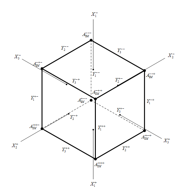
Figure 1: The relations (3.15) represented by a cuboid, in which the $X$’s are represented by the faces of the cuboid, the $Y$’s are represented by the edges, and the functions $A_{\text{YM}}^{\chi_{1}\chi_{2}\chi_{3}}$ ($\chi_{i}=+$ or $-$) are represented by the vertices. Each $A_{\text{YM}}^{\chi_{1}\chi_{2}\chi_{3}}$ is associated with three faces and three edges to which the corresponding vertex is attached. Each vertex is a sum of the associated faces multiplied by perpendicular edges.

Although we have obtained the solution (3.16), we still need to impose the condition that $f_{X}(A_{\text{YM}}^{\chi_{1}\chi_{2}\chi_{3}})$ be a polynomial in $X$’s and $Y$’s. We can set 5 of the $Y$’s to zero such that the 7 of the $A_{\text{YM}}^{\chi_{1}\chi_{2}\chi_{3}}$ are still linearly independent. In this way the remaining $Y$’s can be expressed as linear combinations of the $A_{\text{YM}}^{\chi_{1}\chi_{2}\chi_{3}}$, and $f_{X}(A_{\text{YM}}^{\chi_{1}\chi_{2}\chi_{3}})$ must be a polynomial in $A_{\text{YM}}^{\chi_{1}\chi_{2}\chi_{3}}$, with rational functions of $X$’s as coefficients. Furthermore the amplitude is homogeneous in $e_{i}^{\pm}$, these rational coefficient functions must therefore be homogeneous in $X_{i}^{\pm}$ and must be of the form

$$\prod_{i=1}^{3}(X_{i}^{+})^{n_{i}^{+}}(X_{i}^{-})^{n_{i}^{-}}~{},$$ (3.17)

where $n_{i}^{\pm}$ being integers. The amplitude can finally be expressed as

$$A=P\left(X,A_{\text{YM}}^{\chi_{1}\chi_{2}\chi_{3}}\right)+\frac{Q\left(X,A_{\text{YM}}^{\chi_{1}\chi_{2}\chi_{3}}\right)}{\displaystyle\prod_{i=1}^{3}(X_{i}^{+})^{m_{i}^{+}}(X_{i}^{-})^{m_{i}^{-}}}$$ (3.18)

where $m_{i}^{+},m_{i}^{-}$ are non-negative integers and $P,Q$ are polynomials in the $X$s and $A_{\text{YM}}^{\chi_{1}\chi_{2}\chi_{3}}$. The polynomial $Q(X,A_{\text{YM}}^{\chi_{1}\chi_{2}\chi_{3}})$ is required not to contain a factor of $X_{i}^{\pm}$.

Let us consider the case where the only non-vanishing $m$ in (3.18) is $m_{3}^{+}=1$:

$$A_{3}^{+}=P_{3}^{+}\left(X,A_{\text{YM}}^{\chi_{1}\chi_{2}\chi_{3}}\right)+\frac{Q_{3}^{+}\left(X,A_{\text{YM}}^{\chi_{1}\chi_{2}\chi_{3}}\right)}{X_{3}^{+}}$$ (3.19)

We note the following identity:

$$X_{1}^{-}X_{2}^{-}{A}_{\text{YM}}^{+++}+X_{1}^{+}X_{2}^{+}{A}_{\text{YM}}^{--+}-X_{1}^{-}X_{2}^{+}{A}_{\text{YM}}^{+-+}-X_{1}^{+}X_{2}^{-}{A}_{\text{YM}}^{-++}\equiv 0\quad(\text{mod }X_{3}^{+})$$

which means that the LHS (denoted by $K_{3}^{+}$) contains a factor $X_{3}^{+}$ when viewed as a polynomial in the $X$s and the $Y$s. Expressing $A_{\text{YM}}^{-++}$ in terms of the other linearly independent $A_{\text{YM}}$’s and $K_{3}^{+}$:

$$A_{\text{YM}}^{-++}=\frac{X_{1}^{-}X_{2}^{-}{A}_{\text{YM}}^{+++}+X_{1}^{+}X_{2}^{+}{A}_{\text{YM}}^{--+}-X_{1}^{-}X_{2}^{+}{A}_{\text{YM}}^{+-+}-K_{3}^{+}}{X_{1}^{+}X_{2}^{+}}$$

we can rewrite $Q_{3}^{+}$ as

$$Q_{3}^{+}(X,A_{\text{YM}}^{+++},A_{\text{YM}}^{++-},A_{\text{YM}}^{--+},A_{\text{YM}}^{+-+},A_{\text{YM}}^{-+-},A_{\text{YM}}^{-++},A_{\text{YM}}^{+--})$$

$$= \sum_{k=0}^{k_{\max}}(K_{3}^{+})^{k}\widetilde{Q}_{k}(X,A_{\text{YM}}^{+++},A_{\text{YM}}^{++-},A_{\text{YM}}^{--+},A_{\text{YM}}^{+-+},A_{\text{YM}}^{-+-},A_{\text{YM}}^{+--})$$

where $\widetilde{Q}_{k}$ are polynomials in $A_{\text{YM}}^{+++},\,A_{\text{YM}}^{++-},\,A_{\text{YM}}^{--+}$, and $A_{\text{YM}}^{+-+},\,A_{\text{YM}}^{-+-},A_{\text{YM}}^{+--}$ , which do not contain a factor $X_{3}^{+}$. Let ${A^{\prime}}_{\text{YM}}^{\chi_{1}\chi_{2}\chi_{3}}\equiv A_{\text{YM}}^{\chi_{1}\chi_{2}\chi_{3}}|_{X_{3}^{+}\rightarrow 0}$, then ${A^{\prime}}_{\text{YM}}^{+++}$, ${A^{\prime}}_{\text{YM}}^{++-}$, ${A^{\prime}}_{\text{YM}}^{--+}$, ${A^{\prime}}_{\text{YM}}^{+-+}$, ${A^{\prime}}_{\text{YM}}^{-+-}$ and ${A^{\prime}}_{\text{YM}}^{+--}$ are linearly independent. Therefore if the coefficients of $\widetilde{Q}_{0}$ are not all zero, we would have

$$\widetilde{Q}_{0}\left(X\big{|}_{X_{3}^{+}\rightarrow 0},{A^{\prime}}_{\text{YM}}^{+++},{A^{\prime}}_{\text{YM}}^{++-},{A^{\prime}}_{\text{YM}}^{--+},{A^{\prime}}_{\text{YM}}^{+-+},{A^{\prime}}_{\text{YM}}^{-+-},{A^{\prime}}_{\text{YM}}^{+--}\right)\neq 0~{}.$$

This indicates that $\widetilde{Q}_{0}\not\equiv 0\,\,(\text{mod }X_{3}^{+})\Rightarrow Q_{3}^{+}\not\equiv 0\,\,(\text{mod }X_{3}^{+})$ which violates our assumption. Hence the term $\widetilde{Q}_{0}$ must vanish and $Q_{3}^{+}$ contains a factor $K_{3}^{+}$. So we have proved that $A_{3}^{+}$ can be written as

$$A_{3}^{+}=P_{3}^{+}\left(X,A_{\text{YM}}^{\chi_{1}\chi_{2}\chi_{3}}\right)+\beta_{3}^{+}\widetilde{P}_{3}^{+}\left(X,A_{\text{YM}}^{\chi_{1}\chi_{2}\chi_{3}}\right)$$ (3.20)

where $\widetilde{P}_{3}^{+}$ is a polynomial in the $X$s and $A_{\text{YM}}^{\chi_{1}\chi_{2}\chi_{3}}$, and $\beta_{3}^{+}$ is defined by

$$\beta_{3}^{+} \equiv\frac{X_{1}^{-}X_{2}^{-}A_{\text{YM}}^{+++}+X_{1}^{+}X_{2}^{+}A_{\text{YM}}^{--+}-X_{1}^{-}X_{2}^{+}A_{\text{YM}}^{+-+}-X_{1}^{+}X_{2}^{-}A_{\text{YM}}^{-++}}{X_{3}^{+}}$$

$$=(e_{1}^{+}\cdot p_{2})(e_{2}^{+}\cdot p_{3})(e_{1}^{-}\cdot e_{2}^{-})-(e_{1}^{-}\cdot p_{2})(e_{2}^{+}\cdot p_{3})(e_{1}^{+}\cdot e_{2}^{-})$$

$$-\,(e_{1}^{+}\cdot p_{2})(e_{2}^{-}\cdot p_{3})(e_{1}^{-}\cdot e_{2}^{+})+(e_{1}^{-}\cdot p_{2})(e_{2}^{-}\cdot p_{3})(e_{1}^{+}\cdot e_{2}^{+})$$

Likewise we can show that a generic amplitude (3.18) can be cast into the following form,

$$A=P\left(X,A_{\text{YM}}^{\chi_{1}\chi_{2}\chi_{3}}\right)+\prod_{i=1}^{3}(\beta_{i}^{+})^{m_{i}^{+}}(\beta_{i}^{-})^{m_{i}^{-}}\widetilde{P}\left(X,A_{\text{YM}}^{\chi_{1}\chi_{2}\chi_{3}}\right)$$ (3.21)

where $m_{i}^{\pm}$ are non-negative integers, $\widetilde{P}$ is a polynomial in the $X$’s and $A_{\text{YM}}^{\chi_{1}\chi_{2}\chi_{3}}$, and

$$\left\{\begin{aligned} &\beta_{1}^{\pm}\equiv\frac{X_{2}^{-}X_{3}^{-}A_{\text{YM}}^{\pm++}-X_{2}^{+}X_{3}^{-}A_{\text{YM}}^{\pm-+}+X_{2}^{+}X_{3}^{+}A_{\text{YM}}^{\pm--}-X_{2}^{-}X_{3}^{+}A_{\text{YM}}^{\pm+-}}{X_{1}^{\pm}}\\ &\beta_{2}^{\pm}\equiv\frac{X_{1}^{-}X_{3}^{-}A_{\text{YM}}^{+\pm+}-X_{1}^{+}X_{3}^{-}A_{\text{YM}}^{-\pm+}+X_{1}^{+}X_{3}^{+}A_{\text{YM}}^{-\pm-}-X_{1}^{-}X_{3}^{+}A_{\text{YM}}^{+\pm-}}{X_{2}^{\pm}}\\ &\beta_{3}^{\pm}\equiv\frac{X_{1}^{-}X_{2}^{-}A_{\text{YM}}^{++\pm}-X_{1}^{-}X_{2}^{+}A_{\text{YM}}^{+-\pm}+X_{1}^{+}X_{2}^{+}A_{\text{YM}}^{--\pm}-X_{1}^{+}X_{2}^{-}A_{\text{YM}}^{-+\pm}}{X_{3}^{\pm}}\\ \end{aligned}\right.$$ (3.22)

Staring at the figure 1, the form of the other $\beta$’s can be easily inferred from $\beta_{3}^{+}$. Since $\beta_{i}^{+}=\beta_{i}^{-}$, we can set $\beta_{i}\equiv\beta_{i}^{+}=\beta_{i}^{-}$. We can conclude from (3.21) that the set of all gauge invariant 3-point amplitudes are thus given by

$$A\in\mathbb{C}[A_{\text{YM}}^{\chi_{1}\chi_{2}\chi_{3}},X_{i}^{\pm},\beta_{i}]~{}.$$ (3.23)

With $\beta_{i}$ being antisymmetric in $e_{j}^{+}$ and $e_{j}^{-}$, $j\neq i$. If we restrict to the totally symmetric case (3.1), the set (3.23) reduces to $\mathbb{C}\left[A_{\text{YM}}^{\chi_{1}\chi_{2}\chi_{3}},X_{i}^{\chi_{i}}\right]$, with fixed $\chi_{1},\chi_{2},\chi_{3}$. That’s why $\beta_{i}$ does not show up in equation (3.2).

3.2.3 Helicity Amplitudes

Now let us express the amplitudes in terms of helicity spinors. If there is no $\beta_{i}$ or self contraction terms $e^{+}_{i}\cdot e^{-}_{i}$, then an amplitude $A[\epsilon_{1}(r_{1},\sigma_{1};\lambda_{1}),\epsilon_{2}(r_{2},\sigma_{2};\lambda_{2}),\epsilon_{3}(r_{3},\sigma_{3};\lambda_{3})]$ can be expressed as a polynomial in $X_{i}^{\pm}$ and $A_{\text{YM}}(e_{1}^{\pm},e_{2}^{\pm},e_{3}^{\pm})$. Adopting the convention in the literature [10],

$$p^{\alpha\dot{\alpha}}=p\rangle[p,\quad\quad\left[\epsilon_{p}^{-}(r)\right]^{\alpha\dot{\alpha}}=\sqrt{2}\frac{p\rangle[r}{[pr]},\quad\quad\left[\epsilon_{p}^{+}(r)\right]^{\alpha\dot{\alpha}}=\sqrt{2}\frac{r\rangle[p}{\langle rp\rangle},$$

we have,

$$\begin{array}[]{lll}X_{1}^{+}\propto\dfrac{[12][31]}{[23]},&X_{2}^{+}\propto\dfrac{[12][23]}{[31]},&X_{3}^{+}\propto\dfrac{[31][23]}{[12]}\\ X_{1}^{-}\propto\dfrac{\langle 12\rangle\langle 31\rangle}{\langle 23\rangle},&X_{2}^{-}\propto\dfrac{\langle 12\rangle\langle 23\rangle}{\langle 31\rangle},&X_{3}^{-}\propto\dfrac{\langle 31\rangle\langle 23\rangle}{\langle 12\rangle}\\ A_{\text{YM}}(e_{1}^{+},e_{2}^{+},e_{3}^{-})\propto\dfrac{[12]^{3}}{[31][23]}&A_{\text{YM}}(e_{1}^{+},e_{2}^{-},e_{3}^{+})\propto\dfrac{[31]^{3}}{[12][23]}&A_{\text{YM}}(e_{1}^{-},e_{2}^{+},e_{3}^{+})\propto\dfrac{[23]^{3}}{[12][31]}\\ A_{\text{YM}}(e_{1}^{-},e_{2}^{-},e_{3}^{+})\propto\dfrac{\langle 12\rangle^{3}}{\langle 31\rangle\langle 23\rangle}&A_{\text{YM}}(e_{1}^{-},e_{2}^{+},e_{3}^{-})\propto\dfrac{\langle 31\rangle^{3}}{\langle 12\rangle\langle 23\rangle}&A_{\text{YM}}(e_{1}^{+},e_{2}^{-},e_{3}^{-})\propto\dfrac{\langle 23\rangle^{3}}{\langle 12\rangle\langle 31\rangle}\\ A_{\text{YM}}(e_{1}^{+},e_{2}^{+},e_{3}^{+})=0&A_{\text{YM}}(e_{1}^{-},e_{2}^{-},e_{3}^{-})=0&\end{array}$$ (3.24)

From (3.24) we can see that a term in the polynomial can be a product of only square brackets (the first and the third row of (3.24)), or a product of only angle brackets (the second and the fourth row of (3.24)), or a product of square brackets and angle brackets. The last type vanishes on-shell because the three on-shell momenta satisfy momentum conservation.

The amplitudes can, thus, be written in the form

$$A[\epsilon_{1}(r_{1},\sigma_{1};\lambda_{1}),\epsilon_{2}(r_{2},\sigma_{2};\lambda_{2}),\epsilon_{3}(r_{3},\sigma_{3};\lambda_{3})]$$ (3.25)

$$= \alpha_{S}{X_{1}^{+}}^{a_{1}^{+}}{X_{2}^{+}}^{a_{2}^{+}}{X_{3}^{+}}^{a_{3}^{+}}A_{\text{YM}}(e_{1}^{+},e_{2}^{+},e_{3}^{-})^{b^{++-}}A_{\text{YM}}(e_{1}^{+},e_{2}^{-},e_{3}^{+})^{b^{+-+}}A_{\text{YM}}(e_{1}^{-},e_{2}^{+},e_{3}^{+})^{b^{-++}}$$

$$+\alpha_{A}{X_{1}^{-}}^{a_{1}^{-}}{X_{2}^{-}}^{a_{2}^{-}}{X_{3}^{-}}^{a_{3}^{-}}A_{\text{YM}}(e_{1}^{-},e_{2}^{-},e_{3}^{+})^{b^{--+}}A_{\text{YM}}(e_{1}^{-},e_{2}^{+},e_{3}^{-})^{b^{-+-}}A_{\text{YM}}(e_{1}^{+},e_{2}^{-},e_{3}^{-})^{b^{+--}}$$

$$+\text{VT...}$$

$$= \alpha^{\prime}_{S}[12]^{\sigma_{1}+\sigma_{2}-\sigma_{3}}[23]^{\sigma_{2}+\sigma_{3}-\sigma_{1}}[31]^{\sigma_{3}+\sigma_{1}-\sigma_{2}}+\alpha^{\prime}_{A}\langle 12\rangle^{-\sigma_{1}-\sigma_{2}+\sigma_{3}}\langle 23\rangle^{-\sigma_{2}-\sigma_{3}+\sigma_{1}}\langle 31\rangle^{-\sigma_{3}-\sigma_{1}+\sigma_{2}}$$

where $\alpha_{S},\alpha_{A},\alpha^{\prime}_{S},\alpha^{\prime}_{A}$ are numerical constants to be specified by the underlying theories, and

$$\left\{\begin{aligned} &b^{++-}=\frac{r_{3}-\sigma_{3}}{2},b^{+-+}=\frac{r_{2}-\sigma_{2}}{2},b^{-++}=\frac{r_{1}-\sigma_{1}}{2}\\ &a_{i}^{+}=r_{i}-\frac{\sum_{i}r_{i}-\sum_{i}\sigma_{i}}{2}\qquad(i=1,2,3)\end{aligned}\right.$$ (3.26)

$$\left\{\begin{aligned} &b^{--+}=\frac{r_{3}+\sigma_{3}}{2},b^{-+-}=\frac{r_{2}+\sigma_{2}}{2},b^{+--}=\frac{r_{1}+\sigma_{1}}{2}\\ &a_{i}^{-}=r_{i}-\frac{\sum_{i}r_{i}+\sum_{i}\sigma_{i}}{2}\qquad(i=1,2,3)\end{aligned}\right.$$ (3.27)

and $\{VT...\}$ stands for “terms vanishing on-shell”. This coincides with the general form of three point amplitudes given by Benincasa and Cachazo [5].

The requirement, $a_{1}^{+},a_{2}^{+},a_{3}^{+},b^{++-},b^{+-+},b^{-++}\geqslant 0$, yields

$$\left\{\begin{aligned} &\sigma_{i}\leqslant r_{i}\quad(i=1,2,3)\\ &\sum_{i}\sigma_{i}\geqslant\sum_{i}r_{i}-2\min(r_{1},r_{2},r_{3})\end{aligned};\right.$$ (3.28)

and $a_{1}^{-},a_{2}^{-},a_{3}^{-},b^{--+},b^{-+-},b^{+--}\geqslant 0$ yields

$$\left\{\begin{aligned} &\sigma_{i}\geqslant-r_{i}\quad(i=1,2,3)\\ &\sum_{i}\sigma_{i}\leqslant-\left[\sum_{i}r_{i}-2\min(r_{1},r_{2},r_{3})\right]\end{aligned}\right.$$ (3.29)

The second inequalities in (3.28) and (3.29) cannot be simultaneously satisfied (unless in the trivial case, $r_{1}=r_{2}=r_{3}=0$, which is not being considered here). This indicates that either $\alpha_{S}$ or $\alpha_{A}$ vanishes. In the case where the coefficient $\alpha_{A}$ vanishes, (3.28) leads to

$$\sum_{i}\sigma_{i}\geqslant\max(s_{1},s_{2},s_{3})\quad(s_{i}\equiv|\sigma_{i}|)~{}.$$ (3.30)

With $\sigma_{1},\sigma_{2},\sigma_{3}$ held fixed, this is a necessary and sufficient condition for the existence of non-vanishing $\alpha_{S}$: if we choose $r_{1}=r_{2}=r_{3}=\max(s_{1},s_{2},s_{3})$, then the condition (3.30) implies  (3.28).

Similarly, the necessary and sufficient condition for the existence of non-vanishing $\alpha_{A}$ is

$$\sum_{i}\sigma_{i}\leqslant-\max(s_{1},s_{2},s_{3})~{}.$$ (3.31)

And (3.30) and (3.31) further indicate that the signs of helicities can only be $+++$ or $++-$ for non-vanishing $\alpha_{S}$  (In the latter case, the absolute value of the negative helicity should be less than or equal to the other two helicities.); for non-vanishing $\alpha_{A}$, the signs can only be $---$ or $--+$ (in the latter case, the positive helicity should be less than or equal to the absolute values of the other two helicities).

We pause here to make a few remarks. (3.28) and (3.29) imply that in the case of non-vanishing $\alpha_{S}$, the ranks of the polarization tensors cannot exceed $\sum\sigma_{i}$ and in the case of non-vanishing $\alpha_{A}$, the ranks cannot exceed $-\sum\sigma_{i}$. The inclusion of $\beta_{i}$ has no influence on our discussion since $\beta_{i}$ vanishes in the spinor helicity formalism and will only appear in the $\{VT...\}$ terms. Because a self contraction term $e_{i}^{+}\cdot e_{i}^{-}$ does not affect the helicity, it will not affect (3.30) and (3.31).

The two constraints in (3.30) and (3.31) are absent in the light-cone approach. Thus, we reproduce the mismatch between the covariant approach and the light-cone approach. For further discussions on this mismatch, the readers are referred [19, 21, 23, 22].

One can easily see from (3.25) that the amplitudes are independent of $r_{i}$. This suggests that different representations with the same helicity can give the same amplitudes, as long as the amplitudes for the particular representation exist. But equation (3.25) does not guarantee the existence of non-trivial amplitudes for the representations with mixed symmetries.

3.3 Amplitudes of Polarizations with Mixed Symmetry

We now turn our attention to scattering amplitudes involving tensors with mixed symmetries upon permuting their Lorentz indices. We denote $\bigotimes_{i=1}^{r}e(\mathbf{p},\pi(i))$ by $\hat{\epsilon}(r,\sigma;\pi)$ (with $\sum_{i=1}^{r}\pi(i)=\sigma$ and $\pi$ defined by (2.12)), and denote a general polarization $\sum_{\pi}\lambda(\pi)\hat{\epsilon}(r,\sigma;\pi)$ by $\epsilon(r,\sigma;\lambda)$. Sometimes $\pi$ will also be used to denote the permutations that takes the canonically ordered polarizations

$$\hat{\epsilon}^{0}(r,\sigma)\equiv e(\mathbf{p},+1)\otimes e(\mathbf{p},+1)\cdots e(\mathbf{p},-1)\otimes e(\mathbf{p},-1)$$

into $\hat{\epsilon}(r,\sigma;\pi)$.

From (3.23) we know that the amplitude $A[\hat{\epsilon}_{1}(r_{1},\sigma_{1};\pi_{1}),\hat{\epsilon}_{2}(r_{2},\sigma_{2};\pi_{2}),\hat{\epsilon}_{3}(r_{3},\sigma_{3};\pi_{3});N]$ can be written as a linear combination of the following expressions with functions, $\tau_{i}$ and $\theta_{i}$, and integers, $d_{i}$:

$$\prod_{k=1}^{\frac{r^{\prime}_{1}-r^{\prime}_{2}-r^{\prime}_{3}+N^{\prime}}{2}}e_{1}(\mathbf{p}_{1},\tau_{1}(k))\cdot p_{2}\prod_{k=1}^{\frac{r^{\prime}_{2}-r^{\prime}_{1}-r^{\prime}_{3}+N^{\prime}}{2}}e_{2}(\mathbf{p}_{2},\tau_{2}(k))\cdot p_{1}\prod_{k=1}^{\frac{r^{\prime}_{3}-r^{\prime}_{1}-r^{\prime}_{2}+N^{\prime}}{2}}e_{3}(\mathbf{p}_{3},\tau_{3}(k))\cdot p_{1}\times$$ (3.32)

$$\prod_{k=1}^{\frac{r^{\prime}_{1}+r^{\prime}_{2}+r^{\prime}_{3}-N^{\prime}}{2}}A_{\text{YM}}\left[e_{1}(\mathbf{p}_{1},\theta_{1}(k)),e_{2}(\mathbf{p}_{2},\theta_{2}(k)),e_{3}(\mathbf{p}_{3},\theta_{3}(k))\right]\cdot\beta_{1}^{d_{1}}\beta_{2}^{d_{2}}\beta_{3}^{d_{3}}$$

where

$$0\leqslant d_{1}+d_{2}\leqslant\frac{r_{3}-|\sigma_{3}|}{2},\,\,0\leqslant d_{1}+d_{3}\leqslant\frac{r_{2}-|\sigma_{2}|}{2},\,\,0\leqslant d_{2}+d_{3}\leqslant\frac{r_{1}-|\sigma_{1}|}{2}$$

$$r^{\prime}_{i}\equiv r_{i}+2d_{i}-2\sum_{j=1}^{3}d_{j},\,\,N^{\prime}\equiv N-2\sum_{j=1}^{3}d_{i}$$

and $\pi_{i},\theta_{i}$ being any functions

$$\tau_{i}:\left\{1,2,\cdots,\frac{2r^{\prime}_{i}-(r^{\prime}_{1}+r^{\prime}_{2}+r^{\prime}_{3}-N^{\prime})}{2}\right\}\rightarrow\{+1,-1\}$$ (3.33)

$$\theta_{i}:\left\{1,2,\cdots,\frac{r^{\prime}_{1}+r^{\prime}_{2}+r^{\prime}_{3}-N^{\prime}}{2}\right\}\rightarrow\{+1,-1\}$$ (3.34)

that satisfy

$$\sum_{k=1}^{\frac{2r^{\prime}_{i}-(r^{\prime}_{1}+r^{\prime}_{2}+r^{\prime}_{3}-N^{\prime})}{2}}\tau_{i}(k)\quad+\sum_{k=1}^{\frac{r^{\prime}_{1}+r^{\prime}_{2}+r^{\prime}_{3}-N^{\prime}}{2}}~{}.\theta_{i}(k)=\sigma_{i}~{}.$$

In order to determine the gauge invariant amplitudes of general polarizations $\epsilon_{1}(r_{1},\sigma_{1};\lambda_{1})$, $\epsilon_{2}(r_{2},\sigma_{2};\lambda_{2})$ and $\epsilon_{3}(r_{3},\sigma_{3};\lambda_{3})$, we first write the amplitudes in the following forms,

$$A[\hat{\epsilon}_{1}(r_{1},\sigma_{1};\pi_{1}),\hat{\epsilon}_{2}(r_{2},\sigma_{2};\pi_{2}),\hat{\epsilon}_{3}(r_{3},\sigma_{3};\pi_{3});N] \equiv\hat{\epsilon}_{1}^{\mu_{1}\cdots\mu_{r_{1}}}\hat{\epsilon}_{2}^{\nu_{1}\cdots\nu_{r_{2}}}\hat{\epsilon}_{3}^{\rho_{1}\cdots\rho_{r_{3}}}\hat{K}_{\mu_{1}\cdots\mu_{r_{1}}\nu_{1}\cdots\nu_{r_{2}}\rho_{1}\cdots\rho_{r_{3}}}$$ (3.35)

$$A[\epsilon_{1}(r_{1},\sigma_{1};\lambda_{1}),\epsilon_{2}(r_{2},\sigma_{2};\lambda_{2}),\,\epsilon_{3}(r_{3},\sigma_{3};\lambda_{3});N] \equiv\epsilon_{1}^{\mu_{1}\cdots\mu_{r_{1}}}\epsilon_{2}^{\nu_{1}\cdots\nu_{r_{2}}}\epsilon_{3}^{\rho_{1}\cdots\rho_{r_{3}}}K_{\mu_{1}\cdots\mu_{r_{1}}\nu_{1}\cdots\nu_{r_{2}}\rho_{1}\cdots\rho_{r_{3}}}$$

then the gauge invariance conditions read

$$\delta_{i}^{\pm}(\hat{\epsilon}_{1}^{\mu_{1}\cdots\mu_{r_{1}}}\hat{\epsilon}_{2}^{\nu_{1}\cdots\nu_{r_{2}}}\hat{\epsilon}_{3}^{\rho_{1}\cdots\rho_{r_{3}}})\hat{K}_{\mu_{1}\cdots\mu_{r_{1}}\nu_{1}\cdots\nu_{r_{2}}\rho_{1}\cdots\rho_{r_{3}}}=0\qquad(i=1,2,3)$$ (3.36)

$$\delta_{i}^{\pm}(\epsilon_{1}^{\mu_{1}\cdots\mu_{r_{1}}}\epsilon_{2}^{\nu_{1}\cdots\nu_{r_{2}}}\epsilon_{3}^{\rho_{1}\cdots\rho_{r_{3}}})K_{\mu_{1}\cdots\mu_{r_{1}}\nu_{1}\cdots\nu_{r_{2}}\rho_{1}\cdots\rho_{r_{3}}}=0\qquad(i=1,2,3)$$ (3.37)

which are linear equations in $\hat{K}$ and $K$.

The solutions to equations (3.36) are given by the linear combinations of (3.32) and equations (3.37), yielding

$$0= \delta_{i}^{\pm}\left[\sum_{\pi_{1}}\lambda_{1}(\pi_{1})\pi_{1}(\hat{\epsilon}^{0}_{1})^{\mu_{1}\cdots\mu_{r_{1}}}\sum_{\pi_{2}}\lambda_{2}(\pi_{2})\pi_{2}(\hat{\epsilon}^{0}_{2})^{\nu_{2}\cdots\nu_{r_{2}}}\sum_{\pi_{3}}\lambda_{3}(\pi_{3})\pi_{3}(\hat{\epsilon}^{0}_{3})^{\rho_{3}\cdots\rho_{r_{3}}}\right]$$ (3.38)

$$\times K_{\mu_{1}\cdots\mu_{r_{1}}\nu_{1}\cdots\nu_{r_{2}}\rho_{1}\cdots\rho_{r_{3}}}$$

$$= \delta_{i}^{\pm}\left[(\hat{\epsilon}_{1}^{0})^{\mu_{1}\cdots\mu_{r_{1}}}(\hat{\epsilon}_{2}^{0})^{\nu_{1}\cdots\nu_{r_{2}}}(\hat{\epsilon}_{3}^{0})^{\rho_{1}\cdots\rho_{r_{3}}}\right]\sum_{\pi_{1}}\sum_{\pi_{2}}\sum_{\pi_{3}}\bigg{\{}\lambda_{1}(\pi_{1})\lambda_{2}(\pi_{2})\lambda_{3}(\pi_{3})$$

$$\times(\pi_{1})^{-1}(\pi_{2})^{-1}(\pi_{3})^{-1}K_{\mu_{1}\cdots\mu_{r_{1}}\nu_{1}\cdots\nu_{r_{2}}\rho_{1}\cdots\rho_{r_{3}}}\bigg{\}}~{}.$$

Comparing these equations with (3.36) we find that the solution space for $K$ can be obtained by acting with the linear operators $\sum_{\pi_{1}}\sum_{\pi_{2}}\sum_{\pi_{3}}\lambda_{1}(\pi_{1})\lambda_{2}(\pi_{2})\lambda_{2}(\pi_{2})(\pi_{1})^{-1}(\pi_{2})^{-1}(\pi_{3})^{-1}$ (which can be singular) on the solution space of (3.36). We thus have

$$A\left[\epsilon_{1}(r_{1},\sigma_{1};\lambda_{1}),\epsilon_{2}(r_{2},\sigma_{2};\lambda_{2}),\epsilon_{3}(r_{3},\sigma_{3};\lambda_{3});N\right]$$ (3.39)

$$= \epsilon_{1}^{\mu_{1}\cdots\mu_{r_{1}}}\epsilon_{2}^{\nu_{1}\cdots\nu_{r_{2}}}\epsilon_{3}^{\rho_{1}\cdots\rho_{r_{3}}}\hat{K}_{\mu_{1}\cdots\mu_{r_{1}}\nu_{1}\cdots\nu_{r_{2}}\rho_{1}\cdots\rho_{r_{3}}}$$

$$= \sum_{\pi_{1}}\sum_{\pi_{2}}\sum_{\pi_{3}}\lambda_{1}(\pi_{1})\lambda_{2}(\pi_{2})\lambda_{3}(\pi_{3})A[\hat{\epsilon}_{1}(r_{1},\sigma_{1};\pi_{1}),\hat{\epsilon}_{2}(r_{2},\sigma_{2};\pi_{2}),\hat{\epsilon}_{3}(r_{3},\sigma_{3};\pi_{3});N]~{}.$$

4 Examples

In this section we present a few concrete examples to illustrate our procedure of constructing gauge invariant amplitudes. With the polarizations denoted by $\epsilon_{1},\epsilon_{2},\epsilon_{3}$, the amplitudes can be classified into different categories labelled by ($\overline{L},\overline{M},\overline{N}$), where $\overline{L}$ denotes the number of Lorentz contractions, $e_{i}^{+}\cdot e_{i}^{-}=\text{const}$, $\overline{M}$ the number of $\beta_{i}$ and $\overline{N}$ the number of $A_{\text{YM}}^{\chi_{1}\chi_{2}\chi_{3}}$ in each term of a given amplitude. This classification includes all possible amplitudes, but those of different types may not be linearly independent (as we will discuss further below). The number of derivatives (denoted by $N$) in each term of an amplitude of type ($\overline{L},\overline{M},\overline{N}$) is given by

$$N=r_{1}+r_{2}+r_{3}-2(\overline{L}+\overline{M}+\overline{N})$$ (4.1)

where $r_{1},r_{2},r_{3}$ are the ranks of the polarizations.

Let us first consider the case

$$\epsilon_{1}=e_{1}^{+}\otimes e_{1}^{-},\epsilon_{2}=e_{2}^{+}\otimes e_{2}^{-},\epsilon_{3}=e_{3}^{+}\otimes e_{3}^{-}~{}.$$ (4.2)

Amplitudes $A(\epsilon_{1},\epsilon_{2},\epsilon_{3})$ are thus (where $C_{i}\equiv e_{i}^{+}\cdot e_{i}^{-}$) classified:

$\begin{array}[]{|c|c|}\hline\cr\text{Categories}&\text{Amplitudes}\\ \hline\cr(0,0,0)&X_{1}^{+}X_{1}^{-}X_{2}^{+}X_{2}^{-}X_{3}^{+}X_{3}^{-}\\ \hline\cr(0,0,1)&\begin{aligned} &X_{1}^{-}X_{2}^{-}X_{3}^{-}A_{\text{YM}}^{+++},\quad X_{1}^{+}X_{2}^{-}X_{3}^{-}A_{\text{YM}}^{-++},\quad X_{1}^{-}X_{2}^{+}X_{3}^{-}A_{\text{YM}}^{+-+},\quad X_{1}^{-}X_{2}^{-}X_{3}^{+}A_{\text{YM}}^{++-}\\ &X_{1}^{-}X_{2}^{+}X_{3}^{+}A_{\text{YM}}^{+--},\quad X_{1}^{+}X_{2}^{-}X_{3}^{+}A_{\text{YM}}^{-+-},\quad X_{1}^{+}X_{2}^{+}X_{3}^{-}A_{\text{YM}}^{--+}\end{aligned}\\ \hline\cr(0,0,2)&A_{\text{YM}}^{+++}A_{\text{YM}}^{---},\quad A_{\text{YM}}^{-++}A_{\text{YM}}^{+--},\quad A_{\text{YM}}^{+-+}A_{\text{YM}}^{-+-},\quad A_{\text{YM}}^{++-}A_{\text{YM}}^{--+}\\ \hline\cr(0,1,0)&\beta_{1}X_{1}^{+}X_{1}^{-},\quad\beta_{2}X_{2}^{+}X_{2}^{-},\quad\beta_{3}X_{3}^{+}X_{3}^{-}\\ \hline\cr(1,0,0)&C_{1}X_{2}^{+}X_{2}^{-}X_{3}^{+}X_{3}^{-},\quad C_{2}X_{3}^{+}X_{3}^{-}X_{1}^{+}X_{1}^{-},\quad C_{3}X_{1}^{+}X_{1}^{-}X_{2}^{+}X_{2}^{-}\\ \hline\cr(1,1,0)&C_{1}\beta_{1},\quad C_{2}\beta_{2},\quad C_{3}\beta_{3}\\ \hline\cr(2,0,0)&C_{2}C_{3}X_{1}^{+}X_{1}^{-},\quad C_{1}C_{3}X_{2}^{+}X_{2}^{-},\quad C_{1}C_{2}X_{3}^{+}X_{3}^{-}\\ \hline\cr(3,0,0)&C_{1}C_{2}C_{3}\\ \hline\cr\end{array}$

Table 1: List$(+-,+-,+-)$

We refer to this list as List$(+-,+-,+-)$.

One may attempt to include another amplitude $X_{1}^{+}X_{2}^{+}X_{3}^{+}A_{\text{YM}}^{---}$ of type (0,0,1) in the above list but, as we have mentioned before, it has linear dependence on the other seven amplitudes of the same type, namely,

$$X_{1}^{+}X_{2}^{+}X_{3}^{+}A_{\text{YM}}^{---} =X_{1}^{-}X_{2}^{-}X_{3}^{-}A_{\text{YM}}^{+++}-X_{1}^{+}X_{2}^{-}X_{3}^{-}A_{\text{YM}}^{-++}-X_{1}^{-}X_{2}^{+}X_{3}^{-}A_{\text{YM}}^{+-+}-X_{1}^{-}X_{2}^{-}X_{3}^{+}A_{\text{YM}}^{++-}$$

$$+X_{1}^{-}X_{2}^{+}X_{3}^{+}A_{\text{YM}}^{+--}+X_{1}^{+}X_{2}^{-}X_{3}^{+}A_{\text{YM}}^{-+-}+X_{1}^{+}X_{2}^{+}X_{3}^{-}A_{\text{YM}}^{--+}$$

Categories that have a common number $\overline{L}+\overline{M}+\overline{N}$ (or in other words, have the same number of derivatives) contain linearly dependent amplitudes. This happens when amplitudes with a term $\beta_{i}X_{i}^{\pm}$ appear in the list: $\beta_{i}X_{i}^{\pm}$ is a polynomial in $X$s and $A_{\text{YM}}^{\chi_{1}\chi_{2}\chi_{3}}$. Therefore we need to remove all the amplitudes of type (0,1,0).

Let us now determine the gauge invariant amplitudes for the following cases:

$$(1) \epsilon_{1}=e_{1}^{+}\otimes e_{1}^{-}-e_{1}^{-}\otimes e_{1}^{+},\quad\epsilon_{2}=e_{2}^{\chi_{2}}\otimes e_{2}^{\chi_{2}},\quad\epsilon_{3}=e_{3}^{\chi_{3}}\otimes e_{3}^{\chi_{3}}$$ (4.3)

$$(2) \epsilon_{1}=e_{1}^{+}\otimes e_{1}^{-}-e_{1}^{-}\otimes e_{1}^{+},\quad\epsilon_{2}=e_{2}^{+}\otimes e_{2}^{-}-e_{2}^{-}\otimes e_{2}^{+},\quad\epsilon_{3}=e_{3}^{\chi_{3}}\otimes e_{3}^{\chi_{3}}$$

$$(3) \epsilon_{1}=e_{1}^{+}\otimes e_{1}^{-}-e_{1}^{-}\otimes e_{1}^{+},\quad\epsilon_{2}=e_{2}^{+}\otimes e_{2}^{-}-e_{2}^{-}\otimes e_{2}^{+},\quad\epsilon_{3}=e_{3}^{+}\otimes e_{3}^{-}-e_{3}^{-}\otimes e_{3}^{+}~{}.$$

In Case (1), we substitute $e_{2}^{+}\otimes e_{2}^{-}$, in List$(+-,+-,+-)$, by $e_{2}^{\chi_{2}}\otimes e_{2}^{\chi_{2}}$ and $e_{3}^{+}\otimes e_{3}^{-}$ by $e_{3}^{\chi_{3}}\otimes e_{3}^{\chi_{3}}$ to obtain List$(+-,\chi_{2}\chi_{2},\chi_{3}\chi_{3})$, where in each amplitude:

$$\#(e_{1}^{+})=\#(e_{1}^{-})=1,\#(e_{2}^{\chi_{2}})=\#(e_{3}^{\chi_{3}})=2,\#(e_{2}^{\bar{\chi}_{2}})=\#(e_{3}^{\bar{\chi}_{3}})=0~{}.$$

$\chi_{i}$ can be either $+$ or $-$, and $\bar{\chi}_{i}$ denotes the sign opposite to $\chi_{i}$.

We then delete from List$(+-,\chi_{2}\chi_{2},\chi_{3}\chi_{3})$ the amplitudes that are symmetric in $e_{1}^{+}$ and $e_{1}^{-}$ to get the following truncated list,

$\begin{array}[]{|c|c|}\hline\cr\text{Categories}&\text{Amplitudes}\\ \hline\cr(0,0,1)&X_{1}^{-}X_{2}^{\chi_{2}}X_{3}^{\chi_{3}}A_{\text{YM}}^{+\chi_{2}\chi_{3}},\quad X_{1}^{+}X_{2}^{\chi_{2}}X_{3}^{\chi_{2}}A_{\text{YM}}^{-\chi_{2}\chi_{3}}\\ \hline\cr\end{array}$

Table 2: Truncation of List$(+-,\chi_{2}\chi_{2},\chi_{3}\chi_{3})$

A general gauge invariant amplitude of the polarizations in (1) can be obtained by anti-symmetrizing the amplitudes in the list over the indices of $\epsilon_{1}$:

$$A^{(1)}= X_{1}^{-}X_{2}^{\chi_{2}}X_{3}^{\chi_{3}}A_{\text{YM}}^{+\chi_{2}\chi_{3}}-X_{1}^{+}X_{2}^{\chi_{2}}X_{3}^{\chi_{3}}A_{\text{YM}}^{-\chi_{2}\chi_{3}}$$ (4.4)

$$= (p_{3}\cdot\epsilon_{2}\cdot p_{3})(p_{1}\cdot\epsilon_{3}\cdot\epsilon_{1}\cdot p_{2})+(p_{2}\cdot\epsilon_{3}\cdot p_{2})(p_{1}\cdot\epsilon_{2}\cdot\epsilon_{1}\cdot p_{3})$$

Similarly, the gauge invariant amplitudes for Case (2) can be obtained by anti-symmetrizing the amplitudes in the following list over the indices of $\epsilon_{1}$ and then over the indices of $\epsilon_{2}$,

$\begin{array}[]{|c|c|}\hline\cr\text{Categories}&\text{Amplitudes}\\ \hline\cr(0,0,1)&\begin{aligned} &X_{1}^{-}X_{2}^{-}X_{3}^{\chi_{3}}A_{\text{YM}}^{++\chi_{3}},\,\,X_{1}^{+}X_{2}^{-}X_{3}^{\chi_{3}}A_{\text{YM}}^{-+\chi_{3}},\,\,X_{1}^{-}X_{2}^{+}X_{3}^{\chi_{3}}A_{\text{YM}}^{+-\chi_{3}},\,\,X_{1}^{+}X_{2}^{+}X_{3}^{\chi_{3}}A_{\text{YM}}^{--\chi_{3}}\end{aligned}\\ \hline\cr(0,0,2)&A_{\text{YM}}^{++\chi_{3}}A_{\text{YM}}^{--\chi_{3}},\quad A_{\text{YM}}^{-+\chi_{3}}A_{\text{YM}}^{+-\chi_{3}}\\ \hline\cr\end{array}$

Table 3: Truncation of List$(+-,+-,\chi_{3}\chi_{3})$

The result is:

$$\left\{\begin{aligned} &\begin{aligned} A^{(2)}_{\,\,1}=&X_{1}^{+}X_{2}^{+}X_{3}^{\chi_{3}}A_{\text{YM}}^{--\chi_{3}}-X_{1}^{-}X_{2}^{+}X_{3}^{\chi_{3}}A_{\text{YM}}^{+-\chi_{3}}-X_{1}^{+}X_{2}^{-}X_{3}^{\chi_{3}}A_{\text{YM}}^{-+\chi_{3}}+X_{1}^{-}X_{2}^{-}X_{3}^{\chi_{3}}A_{\text{YM}}^{++\chi_{3}}\\ =&(p_{1}\cdot\epsilon_{3}\cdot p_{1})(p_{2}\cdot\epsilon_{1}\cdot\epsilon_{2}\cdot p_{3}),\end{aligned}\\ &\begin{aligned} A^{(2)}_{\,\,2}=&A_{\text{YM}}^{++\chi_{3}}A_{\text{YM}}^{--\chi_{3}}-A_{\text{YM}}^{+-\chi_{3}}A_{\text{YM}}^{-+\chi_{3}}\\ =&2(p_{2}\cdot\epsilon_{1}\cdot\epsilon_{3}\cdot\epsilon_{2}\cdot p_{3}-p_{1}\cdot\epsilon_{3}\cdot\epsilon_{2}\cdot\epsilon_{1}\cdot p_{2}-p_{1}\cdot\epsilon_{3}\cdot\epsilon_{1}\cdot\epsilon_{2}\cdot p_{3})+(\epsilon_{1}^{\mu\nu}\epsilon_{2\mu\nu})(p_{1}\cdot\epsilon_{3}\cdot p_{1})\end{aligned}\end{aligned}\right.$$ (4.5)

Furthermore the amplitudes for Case (3) (if exists) can be obtained from the following list. But as one can check, the amplitudes listed below all vanish upon anti-symmetrization over the indices of $\epsilon_{1}$, $\epsilon_{2}$ and $\epsilon_{3}$.

$\begin{array}[]{|c|c|}\hline\cr\text{Categories}&\text{Amplitudes}\\ \hline\cr(0,0,1)&\begin{aligned} &X_{1}^{-}X_{2}^{-}X_{3}^{-}A_{\text{YM}}^{+++},\quad X_{1}^{+}X_{2}^{-}X_{3}^{-}A_{\text{YM}}^{-++},\quad X_{1}^{-}X_{2}^{+}X_{3}^{-}A_{\text{YM}}^{+-+},\quad X_{1}^{-}X_{2}^{-}X_{3}^{+}A_{\text{YM}}^{++-}\\ &X_{1}^{-}X_{2}^{+}X_{3}^{+}A_{\text{YM}}^{+--},\quad X_{1}^{+}X_{2}^{-}X_{3}^{+}A_{\text{YM}}^{-+-},\quad X_{1}^{+}X_{2}^{+}X_{3}^{-}A_{\text{YM}}^{--+}\end{aligned}\\ \hline\cr(0,0,2)&A_{\text{YM}}^{+++}A_{\text{YM}}^{---},\quad A_{\text{YM}}^{-++}A_{\text{YM}}^{+--},\quad A_{\text{YM}}^{+-+}A_{\text{YM}}^{-+-},\quad A_{\text{YM}}^{++-}A_{\text{YM}}^{--+}\\ \hline\cr\end{array}$

Table 4: Truncation of List$(+-,+-,+-)$

Although in four dimensions an anti-symmetric rank-2 tensor field $A_{\mu\nu}$ is dual to the scalar field $\phi$ in the free theory, as they both describe a spin-0 degree of freedom, they are no longer dual to each other once interaction is introduced. Whereas non-trivial 3-point amplitudes for $A_{\mu\nu}$ self interaction is absent, $\phi^{3}$ can exist and lead to non-trivial amplitudes. This is the result of different gauge transformations for these two fields. As a matter of fact we can view the polarization of the scalar field $\phi$ as $1$ as it does not have any gauge transformations. We could write down an amplitude $1^{3}$ for $\phi^{3}$ (up to a coupling constant). For $A_{\mu\nu}$, its polarization tensor is $\epsilon_{1}=e_{1}^{+}\otimes e_{1}^{-}-e_{1}^{-}\otimes e_{1}^{+}$ in the equivalence class of the 2-dim Levi-Civita tensor. One could contract three Levi-Civita tensors to obtain a non-zero result which could potentially be the amplitudes dual to $\phi^{3}$. But when we express the contraction in terms of $\epsilon_{1\mu\nu}$ $\epsilon_{2\mu\nu}$ $\epsilon_{3\mu\nu}$ , none are gauge invariant. Even if we relax the constraint of parity conservation, allowing the 4-d Levi-Civita tensor $\epsilon_{\mu\nu\rho\sigma}$ to appear in the amplitudes, non-trivial gauge invariant 3-point amplitudes describing $A_{\mu\nu}$ self-interaction do not exist.

If we, however, only consider expressions with many $\epsilon_{\mu\nu}$’s which are polarization tensors for the same momentum $p$, then as long as we contract all indices to obtain scalars, the resultant expressions are always gauge invariant. But this case only appears in the free theory and is not true for an interactive theory since with interaction we always need to construct scalars from different $\epsilon_{i\mu\nu}$ corresponding to momenta $p_{i}$. This is yet another way to see that the duality between rank-2 antisymmetric tensor and scalar fields does not extend to an interactive theory.

Having determined the gauge invariant 3-point amplitudes in the above examples, we shall find the cubic interaction terms from which these amplitudes can be derived. Here we assume that particles with the same kind of polarization tensors are identical and that the polarizations $\epsilon_{1},\epsilon_{2},\epsilon_{3}$ in (4.3) correspond to the fields $\phi_{a}$,$\phi_{b}$,$\phi_{c}$ which satisfy the Lorenz gauge condition:

$$\partial^{\mu}\phi_{k\mu\nu}=\partial^{\nu}\phi_{k\mu\nu}=0\quad(k=a,b,c)$$ (4.6)

This gauge condition is implicitly imposed by equation (2.9). Carrying out the following replacement (where the subscript $i$ of $(\partial_{\mu})_{i}$ indicates which field the partial derivative acts upon),

$$\begin{array}[]{lll}\epsilon_{1\mu\nu}\rightarrow\phi_{a\mu\nu}&\epsilon_{2\mu\nu}\rightarrow\phi_{b\mu\nu}&\epsilon_{3\mu\nu}\rightarrow\phi_{c\mu\nu}\\ \,\,p_{\mu}\,\,\rightarrow(\partial_{\mu})_{a}&\,\,q_{\mu}\,\,\rightarrow(\partial_{\mu})_{b}&\,\,k_{\mu}\,\,\rightarrow(\partial_{\mu})_{c}\end{array}$$ (4.7)

we obtain the interaction terms tabulated below,

$$\begin{array}[]{|c|c|}\hline\cr\text{amplitude}&\text{interaction term}\\ \hline\cr A^{(1)}&f^{abc}\left[(\partial^{\kappa}\phi_{b}^{\mu\nu})(\partial_{\nu}\partial_{\mu}\phi_{c}^{\rho\sigma})(\partial_{\rho}\phi_{a\sigma\kappa})+(\partial^{\kappa}\phi_{c}^{\mu\nu})(\partial_{\nu}\partial_{\mu}\phi_{b}^{\rho\sigma})(\partial_{\rho}\phi_{a}^{\sigma\kappa})\right]\\ \hline\cr A^{(2)}_{\,\,1}&f^{abc}(\partial_{\mu}\partial_{\nu}\phi_{a}^{\rho\sigma})(\partial_{\rho}\phi_{b\sigma\kappa})(\partial^{\kappa}\phi_{c}^{\mu\nu})\\ \hline\cr A^{(2)}_{\,\,2}&\begin{aligned} f^{abc}&\Big{[}2\phi_{a\mu\nu}(\partial^{\mu}\phi_{b\rho\sigma})(\partial^{\sigma}\phi_{c}^{\nu\rho})-2\phi_{c\mu\nu}(\partial^{\mu}\phi_{a\rho\sigma})(\partial^{\sigma}\phi_{b}^{\nu\rho})-2\phi_{b\rho\sigma}(\partial^{\mu}\phi_{a}^{\nu\rho})(\partial^{\sigma}\phi_{c\mu\nu})\\ &+(\partial_{\rho}\partial_{\sigma}\phi_{a}^{\mu\nu})\phi_{b\mu\nu}\phi_{c}^{\rho\sigma}\Big{]}\end{aligned}\\ \hline\cr\end{array}$$

Because of the gauge condition (4.6), the form of these interaction terms is not unique – a term

$$(\cdots\phi_{a}^{\cdots\mu\cdots}\cdots\partial_{\mu}\phi_{b}^{\cdots}\cdots\phi_{c}^{\cdots})$$

can be changed into

$$-(\cdots\phi_{a}^{\cdots\mu\cdots}\cdots\phi_{b}^{\cdots}\cdots\partial_{\mu}\phi_{c}^{\cdots})$$

by integration by parts. This corresponds to the fact that $p_{2\mu}\epsilon_{1}^{\cdots\mu\cdots}=-p_{3\mu}\epsilon_{1}^{\cdots\mu\cdots}$.

Our previous discussions are all based on on-shell gauge invariance. If we go off-shell, then further information about the interactions can be obtained. For example, we have obtained from on-shell gauge invariance the Yang-Mills amplitude, which allows us to determine the Yang-Mills Lagrangian up to cubic terms:

$$\mathcal{L}=-\frac{1}{4}(\partial_{\mu}A_{\nu}^{a}-\partial_{\nu}A_{\mu}^{a})(\partial^{\mu}A^{a\nu}-\partial^{\nu}A^{a\mu})-gf^{abc}(\partial_{\mu}A^{a}_{\nu})A^{b\mu}A^{c\nu}$$ (4.8)

with $f^{abc}$ being antisymmetric. Under the off-shell version of the leading order gauge transformation we have mentioned, the second term in the Lagrangian will not be invariant:

$$\delta\left[-gf^{abc}(\partial_{\mu}A^{a}_{\nu})A^{b\mu}A^{c\nu}\right]$$ (4.9)

$$\rightarrow gf^{abc}\left[2\xi^{c}\partial_{\mu}\partial_{\nu}(A^{b\mu}A^{a\nu})+\xi^{c}\partial^{\mu}(\partial_{\mu}A_{\nu}^{b}A^{a\nu})-\xi^{c}\partial_{\nu}(\partial_{\mu}A^{b\mu}A^{a\nu})\right]$$

$$= gf^{abc}\xi^{c}(\partial^{2}A_{\nu}^{b})A^{a\nu}$$

where the right arrow indicates that we have performed integration by parts. To compensate for this term, we have to add in the gauge transformation an extra term to make the change of the kinetic term first order in $g$. This extra term must be bilinear in $A_{\mu}^{a}$ and $\xi^{a}$:

$$\delta A_{\mu}^{a}=\partial_{\mu}\xi^{a}+gF^{abc}A_{\mu}^{b}\xi^{c}$$ (4.10)

where $F^{abc}$ are constants to be determined. Then the variation of the kinetic term becomes

$$\delta\left[-\frac{1}{4}(\partial_{\mu}A_{\nu}^{a}-\partial_{\nu}A_{\mu}^{a})(\partial^{\mu}A^{a\nu}-\partial^{\nu}A^{a\mu})\right]$$ (4.11)

$$\rightarrow gF^{abc}\xi^{c}\left\{\partial^{2}A^{a\nu}A_{\nu}^{b}-\left[\partial_{\mu}\partial_{\nu}A^{a\mu}A^{b\nu}+(\mu\leftrightarrow\nu)]\right]\right\}$$

Now that (4.9)+(4.11)=0, we have $F^{abc}=f^{abc}$. We only focus on the on-shell case and will not explore this further. For more discussions on this topic, see e.g. [14].

5 Conclusion and Discussion

We found that under the assumptions of locality, Lorentz invariance and parity conservation, a general three-point amplitude of massless higher-spin gauge bosons can be written as a polynomial in $A_{\text{YM}}^{\chi_{1}\chi_{2}\chi_{3}}$, $X_{i}=e_{i}\cdot p_{j}^{\pm}$, $\beta_{i}$ (as defined by (3.22)), and self contraction terms $e_{i}^{+}\cdot e_{i}^{-}$. For a quantum field theory in four dimensional flat spacetime – either renormalizable or non-renormalizable–the interaction terms are narrowed down (at least in cubic vertices) by the Lorentz invariance and locality properties to only a few choices. This is not only a perturbative, but also a non-perturbative constraint.

If the polarizations are totally symmetric, then the $\beta_{i}$ terms vanish. For three particular polarizations, the possible amplitudes are determined by equation (3.39) as illustrated in Section 4. We also computed explicitly the helicity amplitudes to show that the helicities must satisfy (3.30) or (3.31) for the amplitudes to be nontrivial.

The amplitudes for totally symmetric polarizations $\epsilon^{\pm}_{i}(p)=\bigotimes_{i=1}^{s}e^{\pm}_{i}(p)$ are given by

$$A(\epsilon_{1},\epsilon_{2},\epsilon_{3};N)$$ (5.1)

$$= (e_{1}\cdot p_{2})^{\frac{s_{1}-s_{2}-s_{3}+N}{2}}(e_{2}\cdot p_{1})^{\frac{s_{2}-s_{1}-s_{3}+N}{2}}(e_{3}\cdot p_{1})^{\frac{s_{3}-s_{1}-s_{2}+N}{2}}A_{\text{YM}}(e_{1},e_{2},e_{3})^{\frac{s_{1}+s_{2}+s_{3}-N}{2}}$$

where $N$ is the total number of derivatives in the cubic vertex and

$$A_{\text{YM}}(e_{1},e_{2},e_{3})\equiv(e_{1}\cdot p_{2})(e_{2}\cdot e_{3})-(e_{2}\cdot p_{1})(e_{1}\cdot e_{3})+(e_{3}\cdot p_{1})(e_{1}\cdot e_{2})$$ (5.2)

In 4-dimension, however, due to a Schouten-like identity, the non-trivial amplitudes are given by (assuming $s_{1}\leq s_{2}\leq s_{3}$ for convenience)

$$(e_{1}\cdot p_{2})^{s_{1}}(e_{2}\cdot p_{1})^{s_{2}}(e_{3}\cdot p_{1})^{s_{3}},\quad(e_{2}\cdot p_{1})^{s_{2}-s_{1}}(e_{3}\cdot p_{1})^{s_{3}-s_{1}}A_{YM}^{s_{1}}$$ (5.3)

The amplitudes involving the second rank totally symmetric polarizations $e_{i}\otimes e_{i}\,\,(i=1,2,3)$ are of particular interest, because they are related to gravity.

$$A_{\text{YM}}^{2}(e_{1},e_{2},e_{3}),\quad(e_{1}\cdot p_{2})^{2}(e_{2}\cdot p_{3})^{2}(e_{3}\cdot p_{1})^{2}$$

with momentum number $N=2$, $N=6$, respectively. A few remarks are due:

• In the case of $N=2$, the amplitude can be written as a product of two Yang-Mills amplitudes, which is consistent with the Einstein-Hilbert action. It was shown by Boels and Medina [7] that higher-point Einstein-Hilbert amplitudes can be obtained from the 3-point amplitude by imposing the symmetry and unitarity conditions. Furthermore this is the only amplitude (among the two possible ones that we found here) that corresponds to a constructible theory [5], and as predicted by the famous KLT relation between open and closed strings [24].

• In the case of $N=6$, the amplitude–similar to the Einstein-Hilbert case–is symmetric under permutations of the particles, thus the particle can be a singlet.

Similar to the case of rank-2 tensors, the possible amplitudes of three totally symmetric polarizations of rank-$r$ tensors are given by

$$A_{\text{YM}}^{r}(e_{1},e_{2},e_{3}),\quad(e_{1}\cdot p_{2})^{r}(e_{2}\cdot p_{3})^{r}(e_{3}\cdot p_{1})^{r}$$ (5.4)

When $r$ is even, (5.4) is symmetric under permutations of the particles and the particles in the theory can be a singlet; when $r$ is odd, (5.4) is antisymmetric and the theory is Yang-Mills like, i.e. carrying color indices.

In 4-dimension, massless mixed-symmetry fields can be dualized to totally symmetric fields in the free theory. Our analysis shows that this duality does not extend to the interacting theory. There exists a mismatch between the 3-point amplitudes and thus the cubic interactions of these two fields cannot be dual to each other. To be more precise, in the case of the antisymmetric rank-2 field $A_{\mu\nu}$, although it is dual to the scalar field $\phi$ which enjoys a non-trivial 3-point amplitude, we cannot find a non-trivial 3-point amplitude for $A_{\mu\nu}$, even if we relax our assumption on the parity conservation. Furthermore by expressing our results in spinor helicity formalism we can show that if, for two representations of the same helicity, the 3-point amplitudes for a given total number of derivatives do exist on both sides, then we do expect these particular cubic interactions to be dual to each other, as the 3-point amplitudes in spinor helicity formalism only depend on the helicity.

To obtain, within this framework, further information about the underlying field theories, e.g. the Jacobi identity satisfied by the coupling constants in a Yang-Mills-like theory, it is necessary to extend our method and investigation to four- or higher-point amplitudes. Also, it is interesting to relax the assumption of parity conservation to study the 3-point amplitudes for both totally symmetric fields and the mixed-symmetric fields. We will report our findings in a forthcoming paper.

6 Appendix

In this Appendix, we shall use on-shell gauge invariance to determine the possible 3-point amplitudes of totally symmetric polarizations. Consider three massless particles whose polarization tensors $\epsilon_{1}(p_{1})$, $\epsilon_{2}(p_{2})$, $\epsilon_{3}(p_{3})$ $(p_{1}+p_{2}+p_{3}=0)$ are given by,

$$\epsilon^{\pm}_{1}(p_{1})=\bigotimes_{i=1}^{s_{1}}e^{\pm}_{1}(p_{1}),\quad\epsilon^{\pm}_{2}(p_{2})=\bigotimes_{i=1}^{s_{2}}e^{\pm}_{2}(p_{2}),\quad\epsilon^{\pm}_{3}(p_{3})=\bigotimes_{i=1}^{s_{3}}e^{\pm}_{3}(p_{3})$$ (6.1)

where $s_{i}$ are the spins of the particles and $e_{i}^{\pm}(p_{i})$ the polarization vectors.

A general Lorentz invariant amplitude of these three particles is a homogeneous function of $e_{1}$, $e_{2}$, $e_{3}$ and the momenta of degree $s_{1}$, $s_{2}$, $s_{3}$ and $N$, respectively, which has the form

$$A(\epsilon_{1},\epsilon_{2},\epsilon_{3};N)=\sum_{(l,m,n)\in E}\lambda_{l,m,n}(e_{2}\cdot e_{3})^{l}(e_{1}\cdot e_{3})^{m}(e_{1}\cdot e_{2})^{n}(e_{1}\cdot p_{2})^{s_{1}-m-n}(e_{2}\cdot p_{1})^{s_{2}-l-n}(e_{3}\cdot p_{1})^{s_{3}-l-m}$$ (6.2)

where $N$ satisfies $2|(s_{1}+s_{2}+s_{3}+N)$(that is, $(s_{1}+s_{2}+s_{3}+N)$ is even), $N\leqslant s_{1}+s_{2}+s_{3}$, and

$$E=\left\{(l,m,n)\,\vrule\,m,n,l\in\mathbb{N},l+m+n=\frac{s_{1}+s_{2}+s_{3}-N}{2},m+n\leqslant s_{1},l+n\leqslant s_{2},l+m\leqslant s_{3}\right\}$$

We have included in the amplitude only $N$ number of derivatives because the gauge invariance of the linear combination $\sum_{N}\kappa_{N}A(\epsilon_{1},\epsilon_{2},\epsilon_{3};N)$ is equivalent to the invariance of each $A(\epsilon_{1},\epsilon_{2},\epsilon_{3};N)$. We claim that the necessary and sufficient condition for the existence of a non-vanishing gauge invariant amplitude $A(\epsilon_{1},\epsilon_{2},\epsilon_{3};N)$ is

$$N\geqslant s_{1}+s_{2}+s_{3}-2\min(s_{1},s_{2},s_{3})$$

The proof is as follows.

To simplify the notation, we define

$$\overline{l,m,n}\equiv(e_{2}\cdot e_{3})^{l}(e_{1}\cdot e_{3})^{m}(e_{1}\cdot e_{2})^{n}(e_{1}\cdot p_{2})^{s_{1}-m-n}(e_{2}\cdot p_{1})^{s_{2}-l-n}(e_{3}\cdot p_{1})^{s_{3}-l-m}$$ (6.3)

then the amplitude (6.2) becomes

$$A(\epsilon_{1},\epsilon_{2},\epsilon_{3};N)=\sum_{(l,m,n)\in E}\lambda_{l,m,n}\cdot\overline{l,m,n}$$ (6.4)

The constraints on the integers $l,m,n$ in the set $E$ are equivalent to the following conditions:

$$n =\frac{s_{1}+s_{2}+s_{3}-N}{2}-l-m\equiv n(l,m)$$ (6.5)

$$l \geqslant\max\left(0,\frac{s_{1}+s_{2}+s_{3}-N}{2}-s_{1}\right)$$ (6.6)

$$m \geqslant\max\left(0,\frac{s_{1}+s_{2}+s_{3}-N}{2}-s_{2}\right)$$ (6.7)

$$l +m\leqslant\min\left(s_{3},\frac{s_{1}+s_{2}+s_{3}-N}{2}\right)~{}.$$ (6.8)

We can rewrite the above inequalities in the form

$$\left\{\begin{aligned} l_{\min}^{N}\equiv&\max\left(0,\frac{s_{1}+s_{2}+s_{3}-N}{2}-s_{1}\right)\leqslant l\leqslant\min\left(s_{3},\frac{s_{1}+s_{2}+s_{3}-N}{2}\right)\equiv l_{\max}^{N}\\ m_{\min}^{N}\equiv&\max\left(0,\frac{s_{1}+s_{2}+s_{3}-N}{2}-s_{2}\right)\leqslant m\leqslant\min\left(s_{3},\frac{s_{1}+s_{2}+s_{3}-N}{2}\right)-l\equiv m_{\max}^{N}(l)\end{aligned}\right.$$ (6.9)

Now the equation (6.4) becomes

$$A(\epsilon_{1},\epsilon_{2},\epsilon_{3};N)=\sum_{l=l_{\min}^{N}}^{l_{\max}^{N}}\sum_{m=m_{\min}^{N}}^{m_{\max}^{N}(l)}\lambda_{l,m,n}\cdot\overline{l,m,n}=\sum_{l=l_{\min}^{N}}^{l_{\max}^{N}}A_{l}$$ (6.10)

where

$$A_{l}\equiv\sum_{m=m_{\min}^{N}}^{m_{\max}^{N}(l)}\lambda_{l,m,n}\cdot\overline{l,m,n}$$

The amplitude is invariant under the gauge transformation, $\delta_{1}e_{1}=p_{1},\delta_{1}e_{2}=\delta_{1}e_{3}=0$, (the notation $\delta_{i}e_{j}$ being defined in (2.13)). Because $\delta_{1}A_{l}$ has the structure

$$\delta_{1}A_{l}=\sum_{m}\lambda^{\prime}_{l,m,n}\cdot\overline{l,\times,\times}$$

where $\times$ stands for some numeric constants, we have

$$\delta_{1}A=\sum_{l}\delta_{1}A_{l}=0\,\,\Leftrightarrow\,\,\delta_{1}A_{l}=0\quad(\text{for all }l)$$

Therefore

$$\delta_{1}A_{l} =\sum_{m=m_{\min}^{N}}^{m_{\max}^{N}(l)}(m\lambda_{l,m,n}\cdot\overline{l,m-1,n}+n\lambda_{l,m,n}\cdot\overline{l,m,n-1})$$ (6.11)

$$=\sum_{m=m_{\min}^{N}-1}^{m_{\max}^{N}(l)-1}(m+1)\lambda_{l,m+1,n-1}\cdot\overline{l,m,n-1}+\sum_{m=m_{\min}^{N}}^{m_{\max}^{N}(l)}n\lambda_{l,m,n}\cdot\overline{l,m,n-1}$$ (6.12)

$$=\sum_{m=m_{\min}^{N}}^{m_{\max}^{N}(l)-1}\big{[}(m+1)\lambda_{l,m+1,n-1}+n\lambda_{l,m,n}\big{]}\cdot\overline{l,m,n-1}$$ (6.13)

$$\quad+m_{\min}^{N}\lambda_{l,m_{\min}^{N},n(l,m_{\min}^{N})}\cdot\overline{l,m_{\min}^{N}-1,n(l,m^{N}_{\min})}$$ (6.14)

$$\quad+n(l,m_{\max}^{N}(l))\lambda_{l,m_{\max}^{N}(l),n(l,m_{\max}^{N}(l))}\cdot\overline{l,m_{\max}^{N}(l),n(l,m_{\max}^{N}(l))-1}$$ (6.15)

$$=0$$ (6.16)

which leads to

$$\left\{\begin{aligned} 0&=(m+1)\lambda_{l,m+1,n-1}+n\lambda_{l,m,n}\quad(m_{\min}^{N}\leqslant m\leqslant m_{\max}^{N}(l)-1)\\ 0&=m_{\min}^{N}\lambda_{l,m_{\min}^{N},n(l,m_{\min}^{N})}\\ 0&=n(l,m_{\max}^{N}(l))\lambda_{l,m_{\max}^{N}(l),n(l,m_{\max}^{N}(l))}\end{aligned}\right.$$ (6.17)

Now choose $l$ so that $A_{l}\neq 0$, then we must require

$$m_{\min}^{N}=n(l,m_{max}^{N}(l))=0~{},$$ (6.18)

otherwise we would have, $\lambda_{l,m_{\min}^{N},n(l,m_{\min}^{N})}=0$, or, $\lambda_{l,m_{\max}^{N}(l),n(l,m_{\max}^{N}(l))}=0$, and it follows from the recursion relation, $(m+1)\lambda_{l,m+1,n-1}+n\lambda_{l,m,n}=0$, that all $\lambda_{l,\times,\times}$ vanish. Equations (6.5), (6.9) and (6.18) yield

$$\frac{s_{1}+s_{2}+s_{3}-N}{2}-s_{2}\leqslant 0$$ (6.19)

$$\frac{s_{1}+s_{2}+s_{3}-N}{2}-s_{3}\leqslant 0$$ (6.20)

Similarly, by performing a gauge transformation on particle 2 (or 3) we obtain

$$\frac{s_{1}+s_{2}+s_{3}-N}{2}-s_{1}\leqslant 0$$ (6.21)

The inequalities (6.19), (6.20), and (6.21) can be combined into

$$N\geqslant s_{1}+s_{2}+s_{3}-2\min(s_{1},s_{2},s_{3})$$ (6.22)

which is what we intend to prove. Next we will show that for each $N$ satisfying the above inequality, the amplitude $A(s_{1},s_{2},s_{3};N)$ is unique (up to an overall factor).

With the help of $(\ref{range_of_N})$, the set $E$ becomes

$$E=\left\{(l,m,n)\,\vrule\,m,n,l\in\mathbb{N},l+m+n=\frac{s_{1}+s_{2}+s_{3}-N}{2}\right\}$$ (6.23)

According to equation (6.17) we have

$$\lambda_{l,m,n}\propto\lambda_{l,m+1,n-1}$$ (6.24)

Similarly, by performing a gauge transformation on particle 2 we have

$$\lambda_{l,m,n}\propto\lambda_{l+1,m,n-1}$$ (6.25)

From which we obtain

$$\lambda_{l,m,n}\propto\lambda_{l,0,M-l}\propto\lambda_{l^{\prime},0,M-l^{\prime}}\propto\lambda_{l^{\prime},m^{\prime},n^{\prime}}$$

where $\lambda_{l,m,n}$ and $\lambda_{l^{\prime},m^{\prime},n^{\prime}}$ are any two coefficients and

$$M=\frac{s_{1}+s_{2}+s_{3}-N}{2}~{}.$$

Therefore all the coefficients are proportional to each other. As a result, the amplitude, $A(\epsilon_{1},\epsilon_{2},\epsilon_{3};N)$, is unique up to an overall factor.

It turns out that there are four basic gauge invariant amplitudes, namely, the amplitudes $e_{1}\cdot p_{2}$, $e_{2}\cdot p_{1}$, $e_{3}\cdot p_{1}$ of a spin-1 particle (whose polarization vector is $e_{i},i=1,2,3$) scattering with two scalar particles and the Yang-Mills amplitude $A_{\text{YM}}$:

$$A_{\text{YM}}(e_{1},e_{2},e_{3})\equiv(e_{1}\cdot p_{2})(e_{2}\cdot e_{3})-(e_{2}\cdot p_{1})(e_{1}\cdot e_{3})+(e_{3}\cdot p_{1})(e_{1}\cdot e_{2})~{},$$ (6.26)

from which a general gauge invariant amplitude of particles whose polarizations are $\epsilon_{1},\epsilon_{2}$ and $\epsilon_{3}$ can be uniquely constructed:

$$A(\epsilon_{1},\epsilon_{2},\epsilon_{3};N)$$ (6.27)

$$= (e_{1}\cdot p_{2})^{\frac{s_{1}-s_{2}-s_{3}+N}{2}}(e_{2}\cdot p_{1})^{\frac{s_{2}-s_{1}-s_{3}+N}{2}}(e_{3}\cdot p_{1})^{\frac{s_{3}-s_{1}-s_{2}+N}{2}}A_{\text{YM}}(e_{1},e_{2},e_{3})^{\frac{s_{1}+s_{2}+s_{3}-N}{2}}$$

where the exponents are determined by the requirement that the amplitude have the correct numbers of polarization vectors and momenta: $\#(e_{1})=s_{1},\#(e_{2})=s_{2},\#(e_{3})=s_{3},\sum_{i}\#(p_{i})=N$.