Learning with Average Top-k Loss

Abstract

In this work, we introduce the average top-$k$ (AT_k) loss as a new aggregate loss for supervised learning, which is the average over the $k$ largest individual losses over a training dataset. We show that the AT_k loss is a natural generalization of the two widely used aggregate losses, namely the average loss and the maximum loss, but can combine their advantages and mitigate their drawbacks to better adapt to different data distributions. Furthermore, it remains a convex function over all individual losses, which can lead to convex optimization problems that can be solved effectively with conventional gradient-based methods. We provide an intuitive interpretation of the AT_k loss based on its equivalent effect on the continuous individual loss functions, suggesting that it can reduce the penalty on correctly classified data. We further give a learning theory analysis of MAT_k learning on the classification calibration of the AT_k loss and the error bounds of AT_k-SVM. We demonstrate the applicability of minimum average top-$k$ learning for binary classification and regression using synthetic and real datasets.

1 Introduction

Supervised learning concerns the inference of a function $f:\mathcal{X}\mapsto\mathcal{Y}$ that predicts a target $y\in\mathcal{Y}$ from data/features $\mathbf{x}\in\mathcal{X}$ using a set of labeled training examples $\{(\mathbf{x}_{i},y_{i})\}_{i=1}^{n}$. This is typically achieved by seeking a function $f$ that minimizes an aggregate loss formed from individual losses evaluated over all training samples.

To be more specific, the individual loss for a sample $(\mathbf{x},y)$ is given by $\ell(f(\mathbf{x}),y)$, in which $\ell$ is a nonnegative bivariate function that evaluates the quality of the prediction made by function $f$. For example, for binary classification (i.e., $y_{i}\in\{\pm 1\}$), commonly used forms for individual loss include the $0$-$1$ loss, $\mathbb{I}_{yf(\mathbf{x})\leq 0}$, which is $1$ when $y$ and $f(\mathbf{x})$ have different sign and $0$ otherwise, the hinge loss, $\max(0,1-yf(\mathbf{x}))$, and the logistic loss, $\log_{2}(1+\exp(-yf(\mathbf{x})))$, all of which can be further simplified as the so-called margin loss, i.e., $\ell(y,f(\mathbf{x}))=\ell(yf(\mathbf{x}))$. For regression, squared difference $(y-f(\mathbf{x}))^{2}$ and absolute difference $|y-f(\mathbf{x})|$ are two most popular forms for individual loss, which can be simplified as $\ell(y,f(\mathbf{x}))=\ell(|y-f(\mathbf{x})|)$. Usually the individual loss is chosen to be a convex function of its input, but recent works also propose various types of non-convex individual losses (e.g., he2011maximum ; masnadi2009design ; wu2007robust ; yang2010relaxed ).

The supervised learning problem is then formulated as $\min_{f}\left\{\mathcal{L}(L_{\bf z}(f))+\Omega(f)\right\}$, where $\mathcal{L}(L_{\bf z}(f))$ is the aggregate loss accumulates all individual losses over training samples, i.e., $L_{\bf z}(f)=\{\ell_{i}(f)\}_{i=1}^{n}$, with $\ell_{i}(f)$ being the shorthand notation for $\ell(f(\mathbf{x}_{i}),y_{i})$, and $\Omega(f)$ is the regularizer on $f$. However, in contrast to the plethora of the types of individual losses, there are only a few choices when we consider the aggregate loss:

• the average loss: $\mathcal{L}_{\text{avg}}(L_{\bf z}(f))={1\over n}\sum_{i=1}^{n}\ell_{i}(f)$, i.e., the mean of all individual losses;

• the maximum loss: $\mathcal{L}_{\text{max}}(L_{\bf z}(f))=\max_{1\leq k\leq n}\ell_{i}(f)$, i.e., the largest individual loss;

• the top-$k$ loss shalev2016minimizing : $\mathcal{L}_{\text{top-}k}(L_{\bf z}(f))=\ell_{[k]}(f)$ for $1\leq k\leq n$, i.e., the $k$-th largest (top-$k$) individual loss.

The average loss is unarguably the most widely used aggregate loss, as it is a unbiased approximation to the expected risk and leads to the empirical risk minimization in learning theory bartlett2006convexity ; de2005model ; steinwart2003optimal ; vapnik ; wu2006learning . Further, minimizing the average loss affords simple and efficient stochastic gradient descent algorithms bousquet2008tradeoffs ; srebro2010stochastic . On the other hand, the work in shalev2016minimizing shows that constructing learning objective based on the maximum loss may lead to improved performance for data with separate typical and rare sub-populations. The top-k loss shalev2016minimizing generalizes the maximum loss, as $\mathcal{L}_{\text{max}}(L_{\bf z}(f))=\mathcal{L}_{\text{top-}1}(L_{\bf z}(f))$, and can alleviate the sensitivity to outliers of the latter. However, unlike the average loss or the maximum loss, the top-k loss in general does not lead to a convex learning objective, as it is not convex of all the individual losses $L_{\bf z}(f)$.

In this work, we propose a new type of aggregate loss that we term as the average top-k (AT_k) loss, which is the average of the largest $k$ individual losses, that is defined as:

$$\textstyle\mathcal{L}_{\text{avt-}k}(L_{\bf z}(f))={1\over k}\sum_{i=1}^{k}\ell_{[i]}(f).$$ (1)

We refer to learning objectives based on minimizing the AT_k loss as MAT_k learning.

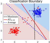
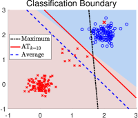
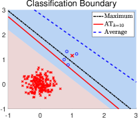
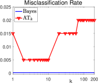
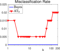
Figure 1: Comparison of different aggregate losses on 2D synthetic datasets with $n=200$ samples for binary classification on a balanced but multi-modal dataset and with outliers (top) and an imbalanced dataset with outliers (bottom) with logistic loss (left) and hinge loss (right). Outliers in data are shown as an enlarged $\times$ and the optimal Bayes classifications are shown as shaded areas. The figures in the second and fourth columns show the misclassification rate of AT_k vs. $k$ for each case.

The AT_k loss generalizes the average loss ($k=n$) and the maximum loss ($k=1$), yet it is less susceptible to their corresponding drawbacks, i.e., it is less sensitive to outliers than the maximum loss and can adapt to imbalanced and/or multi-modal data distributions better than the average loss. This is illustrated with two toy examples of synthesized 2D data for binary classification in Fig.1 (see Appendix  for a complete illustration). As these plots show, the linear classifier obtained with the maximum loss is not optimal due to the existence of outliers while the linear classifier corresponding to the average loss has to accommodate the requirement to minimize individual losses across all training data, and sacrifices smaller sub-clusters of data (e.g., the rare population of $+$ class in the top row and the smaller dataset of $-$ class in the bottom row). In contrast, using AT_k loss with $k=10$ can better protect such smaller sub-clusters and leads to linear classifiers closer to the optimal Bayesian linear classifier. This is also corroborated by the plots of corresponding misclassification rate of AT_k vs. $k$ value in Fig.1, which show that minimum misclassification rates occur at $k$ value other than $1$ (maximum loss) or $n$ (average loss).

The AT_k loss is a tight upper-bound of the top-$k$ loss, as $\mathcal{L}_{\text{avt-}k}(L_{\bf z}(f))\geq\mathcal{L}_{\text{top-}k}(L_{\bf z}(f))$ with equality holds when $k=1$ or $\ell_{i}(f)=$ constant, and it is a convex function of the individual losses (see Section 2). Indeed, we can express $\ell_{[k]}(f)$ as the difference of two convex functions $k\mathcal{L}_{\text{avt-}k}(L_{\bf z}(f))-(k-1)\mathcal{L}_{\text{avt-}(k-1)}(L_{\bf z}(f))$, which shows that in general $\mathcal{L}_{\text{top-}k}(L_{\bf z}(f))$ is not convex with regards to the individual losses.

In sequel, we will provide a detailed analysis of the AT_k loss and MAT_k learning. First, we establish a reformulation of the AT_k loss as the minimum of the average of the individual losses over all training examples transformed by a hinge function. This reformulation leads to a simple and effective stochastic gradient-based algorithm for MAT_k learning, and interprets the effect of the AT_k loss as shifting down and truncating at zero the individual loss to reduce the undesirable penalty on correctly classified data. When combined with the hinge function as individual loss, the AT_k aggregate loss leads to a new variant of SVM algorithm that we term as AT_k SVM, which generalizes the C-SVM and the $\nu$-SVM algorithms scholkopf2000new . We further study learning theory of MAT_k learning, focusing on the classification calibration of the AT_k loss function and error bounds of the AT_k SVM algorithm. This provides a theoretical lower-bound for $k$ for reliable classification performance. We demonstrate the applicability of minimum average top-$k$ learning for binary classification and regression using synthetic and real datasets.

The main contributions of this work can be summarized as follows.

• We introduce the AT_k loss for supervised learning, which can balance the pros and cons of the average and maximum losses, and allows the learning algorithm to better adapt to imbalanced and multi-modal data distributions.

• We provide algorithm and interpretation of the AT_k loss, suggesting that most existing learning algorithms can take advantage of it without significant increase in computation.

• We further study the theoretical aspects of AT_k loss on classification calibration and error bounds of minimum average top-$k$ learning for AT_k-SVM.

• We perform extensive experiments to validate the effectiveness of the MAT_k learning.

2 Formulation and Interpretation

The original AT_k loss, though intuitive, is not convenient to work with because of the sorting procedure involved. This also obscures its connection with the statistical view of supervised learning as minimizing the expectation of individual loss with regards to the underlying data distribution. Yet, it affords an equivalent form, which is based on the following result.

Lemma 1 (Lemma 1, Ogryczak:2003dl ).

$\sum_{i=1}^{k}x_{[i]}$ is a convex function of $(x_{1},\cdots,x_{n})$. Furthermore, for $x_{i}\geq 0$ and $i=1,\cdots,n$, we have $\sum_{i=1}^{k}x_{[i]}=\min_{\lambda\geq 0}\left\{k\lambda+\sum_{i=1}^{n}\left[x_{i}-\lambda\right]_{+}\right\}$, where $\left[a\right]_{+}=\max\{0,a\}$ is the hinge function.

For completeness, we include a proof of Lemma 1 in Appendix. Using Lemma 1, we can reformulate the AT_k loss (1) as

$$\mathcal{L}_{\text{avt-}k}(L_{\bf z}(f))={1\over k}\sum_{i=1}^{k}\ell_{[i]}(f)\propto\min_{\lambda\geq 0}\left\{{1\over n}\sum_{i=1}^{n}\left[\ell_{i}(f)-\lambda\right]_{+}+{k\over n}\lambda\right\}.$$ (2)

In other words, the AT_k loss is equivalent to minimum of the average of individual losses that are shifted and truncated by the hinge function controlled by $\lambda$. This sheds more lights on the AT_k loss, which is particularly easy to illustrate in the context of binary classification using the margin losses, $\ell(f(\mathbf{x}),y)=\ell(yf(\mathbf{x}))$.

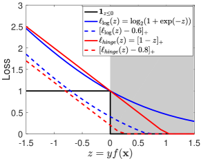
Figure 2: The AT_k loss interpreted at the individual loss level. Shaded area corresponds to data/target with correct classification.

In binary classification, the “gold standard” of individual loss is the $0$-$1$ loss $\mathbb{I}_{yf(\mathbf{x})\leq 0}$, which exerts a constant penalty $1$ to examples that are misclassified by $f$ and no penalty to correctly classified examples. However, the $0$-$1$ loss is difficult to work as it is neither continuous nor convex. In practice, it is usually replaced by a surrogate convex loss. Such convex surrogates afford efficient algorithms, but as continuous and convex upper-bounds of the $0$-$1$ loss, they typically also penalize correctly classified examples, i.e., for $y$ and $\mathbf{x}$ that satisfy $yf(\mathbf{x})>0$, $\ell(yf(\mathbf{x}))>0$, whereas $\mathbb{I}_{yf(\mathbf{x})\leq 0}=0$ (Fig.2). This implies that when the average of individual losses across all training examples is minimized, correctly classified examples by $f$ that are “too close” to the classification boundary may be sacrificed to accommodate reducing the average loss, as is shown in Fig.1.

In contrast, after the individual loss is combined with the hinge function, i.e., $\left[\ell(yf(\mathbf{x}))-\lambda\right]_{+}$ with $\lambda>0$, it has the effect of “shifting down” the original individual loss function and truncating it at zero, see Fig.2. The transformation of the individual loss reduces penalties of all examples, and in particular benefits correctly classified data. In particular, if such examples are “far enough” from the decision boundary, like in the $0$-$1$ loss, their penalty becomes zero. This alleviates the likelihood of misclassification on those rare sub-populations of data that are close to the decision boundary.

Algorithm: The reformulation of the AT_k loss in Eq.(2) also facilitates development of optimization algorithms for the minimum AT_k learning. As practical supervised learning problems usually use a parametric form of $f$, as $f(\mathbf{x};\mathbf{w})$, where $\mathbf{w}$ is the parameter, the corresponding minimum AT_k objective becomes

$$\min_{\mathbf{w},\lambda\geq 0}\left\{{1\over n}\sum_{i=1}^{n}\left[\ell(f(\mathbf{x}_{i};\mathbf{w}),y_{i})-\lambda\right]_{+}+{k\over n}\lambda+\Omega(\mathbf{w})\right\},$$ (3)

It is not hard to see that if $\ell(f(\mathbf{x};\mathbf{w}),y)$ is convex with respect to $\mathbf{w}$, the objective function of in Eq.(3) is a convex function for $\mathbf{w}$ and $\lambda$ jointly. This leads to an immediate stochastic (projected) gradient descent bousquet2008tradeoffs ; srebro2010stochastic for solving (3). For instance, with $\Omega(\mathbf{w})={1\over 2C}\|\mathbf{w}\|^{2}$, where $C>0$ is a regularization factor, at the $t$-th iteration, the corresponding MAT_k objective can be minimized by first randomly sampling $(\mathbf{x}_{i_{t}},y_{i_{t}})$ from the training set and then updating the parameters as

$$\begin{array}[]{ll}\mathbf{w}^{(t+1)}&\leftarrow\mathbf{w}^{(t)}-\eta_{t}\left(\partial_{\mathbf{w}}\ell(f(\mathbf{x}_{i_{t}};\mathbf{w}^{(t)}),y_{i_{t}})\cdot\mathbb{I}_{[\ell(f(\mathbf{x}_{i_{t}};\mathbf{w}^{(t)}),y_{i_{t}})>\lambda^{(t)}]}+{\mathbf{w}^{(t)}\over C}\right)\\ \lambda^{(t+1)}&\leftarrow\left[\lambda^{(t)}-\eta_{t}\left({k\over n}-\mathbb{I}_{[\ell(f(\mathbf{x}_{i_{t}};\mathbf{w}^{(t)},y_{i_{t}})>\lambda^{(t)}]}\right)\right]_{+}\end{array}$$ (4)

where $\partial_{\mathbf{w}}\ell(f(\mathbf{x};\mathbf{w}),y)$ denotes the sub-gradient with respect to $\mathbf{w},$ and $\eta_{t}\sim{1\over\sqrt{t}}$ is the step size.

AT_k-SVM: As a general aggregate loss, the AT_k loss can be combined with any functional form for individual losses. In the case of binary classification, the AT_k loss combined with the individual hinge loss for a prediction function $f$ from a reproducing kernel Hilbert space (RKHS) scholkopf2001learning leads to the AT_k-SVM model. Specifically, we consider function $f$ as a member of RKHS $\mathcal{H}_{K}$ with norm $\|\cdot\|_{K}$, which is induced from a reproducing kernel $K:\mathcal{X}\times\mathcal{X}\to\mathbb{R}$. Using the individual hinge loss, $[1-y_{i}f(\mathbf{x}_{i})]_{+}$, the corresponding MAT_k learning objective in RKHS becomes

$$\min_{f\in\mathcal{H}_{K},\lambda\geq 0}{1\over n}\sum_{i=1}^{n}\left[\left[1-y_{i}f(\mathbf{x}_{i})\right]_{+}-\lambda\right]_{+}+{k\over n}\lambda+\frac{1}{2C}\|f\|^{2}_{K},$$ (5)

where $C>0$ is the regularization factor. Furthermore, the outer hinge function in (5) can be removed due to the following result.

Lemma 2.

For $a\geq 0$, $b\geq 0$, there holds $\left[\left[a-\ell\right]_{+}-b\right]_{+}$ = $\left[a-b-\ell\right]_{+}$.

Proof of Lemma 2 can be found in the Appendix. In addition, note that for any minimizer $(f_{\bf z},\lambda_{\bf z})$ of (5), setting $f(\mathbf{x})=0,\lambda=1$ in the objective function of (5), we have ${k\over n}\lambda_{\bf z}\leq{1\over n}\sum_{i=1}^{n}\left[\left[1-y_{i}f_{\bf z}({\bf x}_{i})\right]_{+}-\lambda_{\bf z}\right]_{+}+{k\over n}\lambda_{\bf z}+\frac{1}{2C}\|f_{\bf z}\|^{2}_{K}\leq{k\over n}$, so we have $0\leq\lambda_{\bf z}\leq 1$ which means that the minimization can be restricted to $0\leq\lambda\leq 1.$ Using these results and introducing $\rho=1-\lambda$, Eq.(5) can be rewritten as

$$\min_{f\in\mathcal{H}_{K},0\leq\rho\leq 1}\ {1\over n}\sum_{i=1}^{n}[\rho-y_{i}f(\mathbf{x}_{i})]_{+}-{k\over n}\rho+\frac{1}{2C}\|f\|^{2}_{K}.$$ (6)

The AT_k-SVM objective generalizes many several existing SVM models. For example, when $k=n$, it equals to the standard C-SVM cortes1995support . When $C=1$ and with conditions $K(\mathbf{x}_{i},\mathbf{x}_{i})\leq 1$ for any $i$, AT_k-SVM reduces to $\nu$-SVM scholkopf2000new with $\nu={k\over n}$. Furthermore, similar to the conventional SVM model, writing in the dual form of (6) can lead to a convex quadratic programming problem that can be solved efficiently. See Appendix  for more detailed explanations.

Choosing $k$. The number of top individual losses in the AT_k loss is a critical parameter that affects the learning performance. In concept, using AT_k loss will not be worse than using average or maximum losses as they correspond to specific choices of $k$. In practice, $k$ can be chosen during training from a validation dataset as the experiments in Section 4. As $k$ is an integer, a simple grid search usually suffices to find a satisfactory value. Besides, Theorem 1 in Section 3 establishes a theoretical lower bound for $k$ to guarantee reliable classification based on the Bayes error. If we have information about the proportion of outliers, we can also narrow searching space of $k$ based on the fact that AT_k loss is the convex upper bound of the top-k loss, which is similar to shalev2016minimizing .

3 Statistical Analysis

In this section, we address the statistical properties of the AT_k objective in the context of binary classification. Specifically, we investigate the property of classification calibration bartlett2006convexity of the AT_k general objective, and derive bounds for the misclassification error of the AT_k-SVM model in the framework of statistical learning theory (e.g.  bartlett2006convexity ; de2005model ; steinwart2008support ; wu2006learning ).

3.1 Classification Calibration under AT_k Loss

We assume the training data ${\bf z}=\{(\mathbf{x}_{i},y_{i})\}_{i=1}^{n}$ are i.i.d. samples from an unknown distribution $p$ on $\mathcal{X}\times\{\pm 1\}$. Let $p_{\mathcal{X}}$ be the marginal distribution of $p$ on the input space $\mathcal{X}$. Then, the misclassification error of a classifier $f:\mathcal{X}\to\{\pm 1\}$ is denoted by ${\mathcal{R}}(f)=\Pr(y\neq f(\mathbf{x}))={\mathbb{E}}[\mathbb{I}_{yf(\mathbf{x})\leq 0}]$. The Bayes error is given by ${\mathcal{R}}^{\ast}=\inf_{f}{\mathcal{R}}(f),$ where the infimum is over all measurable functions. No function can achieve less risk than the Bayes rule $f_{c}(\mathbf{x})=\hbox{sign}(\eta(\mathbf{x})-{1\over 2})$, where $\eta(\mathbf{x})=\Pr(y=1|\mathbf{x})$ devroye2013probabilistic .

In practice, one uses a surrogate loss $\ell:\mathbb{R}\to[0,\infty)$ which is convex and upper-bound the $0$-$1$ loss. The population $\ell$-risk (generalization error) is given by ${\mathcal{E}}_{\ell}(f)={\mathbb{E}}[\ell(yf(x))]$. Denote the optimal $\ell$-risk by ${\mathcal{E}}^{\ast}_{\ell}=\inf_{f}{\mathcal{E}}_{\ell}(f)$. A very basic requirement for using such a surrogate loss $\ell$ is the so-called classification calibration (point-wise form of Fisher consistency) bartlett2006convexity ; lin . Specifically, a loss $\ell$ is classification calibrated with respect to distribution $p$ if, for any $x$, the minimizer $f^{\ast}_{\ell}=\inf_{f}{\mathcal{E}}_{\ell}(f)$ should have the same sign as the Bayes rule $f_{c}(\mathbf{x})$, i.e., $\hbox{sign}(f^{\ast}_{\ell}(\mathbf{x}))=\hbox{sign}(f_{c}(\mathbf{x}))$ whenever $f_{c}(\mathbf{x})\neq 0$.

An appealing result concerning the classification calibration of a loss function $\ell$ was obtained in bartlett2006convexity , which states that $\ell$ is classification calibrated if $\ell$ is convex, differentiable at $0$ and $\ell^{\prime}(0)<0$. In the same spirit, we investigate the classification calibration property of the AT_k loss. Specifically, we first obtain the population form of the AT_k objective using the infinite limit of (2)

$${1\over n}\sum_{i=1}^{n}\left[\ell(y_{i}f(\mathbf{x}_{i}))-\lambda\right]_{+}+{k\over n}\lambda\xrightarrow[n\to\infty]{{k\over n}\to\nu}{\mathbb{E}}\left[[\ell(yf(\mathbf{x}))-\lambda]_{+}\right]+\nu\lambda.$$

We then consider the optimization problem

$$(f^{\ast},\lambda^{\ast})=\arg\inf_{f,\lambda\geq 0}{\mathbb{E}}\left[[\ell(yf(\mathbf{x}))-\lambda]_{+}\right]+\nu\lambda,$$ (7)

where the infimum is taken over all measurable function $f:\mathcal{X}\to\mathbb{R}$. We say the AT_k (aggregate) loss is classification calibrated with respect to $p$ if $f^{\ast}$ has the same sign as the Bayes rule $f_{c}$. The following theorem establishes such conditions.

Theorem 1.

Suppose the individual loss $\ell:\mathbb{R}\to\mathbb{R}^{+}$ is convex, differentiable at $0$ and $\ell^{\prime}(0)<0$. Without loss of generality, assume that $\ell(0)=1$. Let $(f^{\ast},\lambda^{\ast})$ be defined in (7),

• If $\nu>{{\mathcal{E}}^{\ast}_{\ell}}$ then the AT_k loss is classification calibrated.

• If, moreover, $\ell$ is monotonically decreasing and the AT_k aggregate loss is classification calibrated then $\nu\geq\int_{\eta({\bf x})\neq{1\over 2}}\min(\eta(\mathbf{x}),1-\eta(\mathbf{x}))dp_{\mathcal{X}}(\mathbf{x})$.

The proof of Theorem 1 can be found in the Appendix. Part (i) and (ii) of the above theorem address respectively the sufficient and necessary conditions on $\nu$ such that the AT_k loss becomes classification calibrated. Since $\ell$ is an upper bound surrogate of the $0$-$1$ loss, the optimal $\ell$-risk ${\mathcal{E}}^{\ast}_{\ell}$ is larger than the Bayes error ${\mathcal{R}}^{\ast},$ i.e.,  ${\mathcal{E}}^{\ast}_{\ell}\geq{\mathcal{R}}^{\ast}$. In particular, if the individual loss $\ell$ is the hinge loss then ${\mathcal{E}}^{\ast}_{\ell}=2{\mathcal{R}}^{\ast}$. Part (ii) of the above theorem indicates that the AT_k aggregate loss is classification calibrated if $\nu=\lim_{n\to\infty}{k/n}$ is larger than the optimal generalization error ${\mathcal{E}}^{\ast}_{\ell}$ associated with the individual loss. The choice of $k>n{\mathcal{E}}^{\ast}_{\ell}$ thus guarantees classification calibration, which gives a lower bound of $k$. This result also provides a theoretical underpinning of the sensitivity to outliers of the maximum loss (AT_k loss with $k=1$). If the probability of the set $\{x:\eta(x)=1/2\}$ is zero, ${\mathcal{R}}^{\ast}=\int_{\mathcal{X}}\min(\eta(\mathbf{x}),1-\eta(\mathbf{x}))dp_{\mathcal{X}}(\mathbf{x})=\int_{\eta(\mathbf{x})\neq{1/2}}\min(\eta(\mathbf{x}),1-\eta(\mathbf{x}))dp_{\mathcal{X}}(x)$. Theorem 1 indicates that in this case, if the maximum loss is calibrated, one must have ${1\over n}\approx\nu\geq R^{\ast}$. In other words, as the number of training data increases, the Bayes error has to be arbitrarily small, which is consistent with the empirical observation that the maximum loss works well under the well-separable data setting but are sensitive to outliers and non-separable data.

3.2 Error bounds of AT_k-SVM

We next study the excess misclassification error of the AT_k-SVM model i.e.,  ${\mathcal{R}}(\hbox{sign}(f_{\bf z}))-{\mathcal{R}}^{\ast}$. Let $(f_{\bf z},\rho_{\bf z})$ be the minimizer of the AT_k-SVM objective (6) in the RKHS setting. Let $f_{\mathcal{H}}$ be the minimizer of the generalization error over the RKHS space $\mathcal{H}_{K}$, i.e.,  $f_{\mathcal{H}}=\mathop{\arg\!\min}_{f\in\mathcal{H}_{K}}{\mathcal{E}}_{h}(f)$, where we use the notation ${\mathcal{E}}_{h}(f)={\mathbb{E}}\left[[1-yf(\mathbf{x})]_{+}\right]$ to denote the $\ell$-risk of the hinge loss. In the finite-dimension case, the existence of $f_{\mathcal{H}}$ follows from the direct method in the variational calculus, as ${\mathcal{E}}_{h}(\cdot)$ is lower bounded by zero, coercive, and weakly sequentially lower semi-continuous by its convexity. For an infinite dimensional $\mathcal{H}_{K}$, we assume the existence of $f_{\mathcal{H}}$. We also assume that ${\mathcal{E}}_{h}(f_{\mathcal{H}})<1$ since even a naïve zero classifier can achieve ${\mathcal{E}}_{h}(0)=1$. Denote the approximation error by ${\mathcal{A}}(\mathcal{H}_{K})=\inf_{f\in\mathcal{H}_{K}}{\mathcal{E}}_{h}(f)-{\mathcal{E}}_{h}(f_{c})={\mathcal{E}}_{h}(f_{\mathcal{H}})-{\mathcal{E}}_{h}(f_{c})$, and let $\kappa=\sup_{\mathbf{x}\in\mathcal{X}}\sqrt{K(\mathbf{x},\mathbf{x})}$. The main theorem can be stated as follows.

Theorem 2.

Consider the AT_k-SVM in RKHS (6). For any $\varepsilon\in(0,1]$ and $\mu\in(0,1-{\mathcal{E}}_{h}(f_{\mathcal{H}}))$, choosing $k=\lceil n({\mathcal{E}}_{h}(f_{\mathcal{H}})+\mu)\rceil$. Then, it holds

$$\Pr\bigl{\{}{\cal R}(\hbox{sign}(f_{{\bf z}}))-{\mathcal{R}}^{\ast}\geq\mu+{\mathcal{A}}(\mathcal{H})+\varepsilon+{1+C_{\kappa,\mathcal{H}}\over\sqrt{n}\mu}\bigr{\}}\leq 2\exp\bigl{(}-{n\mu^{2}\varepsilon^{2}\over(1+C_{\kappa,\mathcal{H}})^{2}}\bigr{)},$$

where $C_{\kappa,\mathcal{H}}=\kappa(2\sqrt{2C}+4\|f_{\mathcal{H}}\|_{K})$.

The complete proof of Theorem 2 is given in the Appendix. The main idea is to show that $\rho_{\bf z}$ is bounded from below by a positive constant with high probability, and then bound the excess misclassification error ${\mathcal{R}}(\hbox{sign}(f^{\ast}_{\bf z}))-{\mathcal{R}}^{\ast}$ by ${\mathcal{E}}_{h}({f_{\bf z}/\rho_{\bf z}})-{\mathcal{E}}_{h}(f_{c})$. If $K$ is a universal kernel then ${\mathcal{A}}(\mathcal{H}_{K})=0$ steinwart2008support . In this case, let $\mu=\varepsilon\in(0,1-{\mathcal{E}}_{h}(f_{\mathcal{H}}))$, then from Theorem 2 we have

$$\Pr\bigl{\{}{\cal R}(\hbox{sign}(f_{{\bf z}}))-{\mathcal{R}}^{\ast}\geq 2\varepsilon+{1+C_{\kappa,\mathcal{H}}\over\sqrt{n}\varepsilon}\bigr{\}}\leq 2\exp\bigl{(}-{n\varepsilon^{4}\over(1+C_{\kappa,\mathcal{H}})^{2}}\bigr{)},$$

Consequently, choosing $C$ such that $\lim_{n\to\infty}{C/n}=0$, which is equivalent to $\lim_{n\to\infty}{(1+C_{\kappa,\mathcal{H}})^{2}/n}=0$, then ${\cal R}(\hbox{sign}(f_{{\bf z}}))$ can be arbitrarily close to the Bayes error ${\mathcal{R}}^{\ast}$, with high probability, as long as $n$ is sufficiently large.

4 Experiments

We have demonstrated that AT_k loss provides a continuum between the average loss and the maximum loss, which can potentially alleviates their drawbacks. A natural question is whether such an advantage actually benefits practical learning problems. In this section, we demonstrate the behaviors of MAT_k learning coupled with different individual losses for binary classification and regression on synthetic and real datasets, with minimizing the average loss and the maximum loss treated as special cases for $k=n$ and $k=1$, respectively. For simplicity, in all experiments, we use homogenized linear prediction functions $f(\mathbf{x})=\mathbf{w}^{T}\mathbf{x}$ with parameters $\mathbf{w}$ and the Tikhonov regularizer $\Omega(\mathbf{w})={1\over 2C}||\mathbf{w}||^{2}$ , and optimize the MAT_k learning objective with the stochastic gradient descent method given in (4).

Binary Classification: We conduct experiments on binary classification using eight benchmark datasets from the UCI and KEEL data repositories to illustrate the potential effects of using AT_k loss in practical learning to adapt to different underlying data distributions. A detailed description of the datasets is given in Appendix. The standard individual logistic loss and hinge loss are combined with different aggregate losses. Note that average loss combined with individual logistic loss corresponds to the logistic regression model and average loss combined with individual hinge loss leads to the C-SVM algorithm cortes1995support .

For each dataset, we randomly sample 50%, 25%, 25% examples as training, validation and testing sets, respectively. During training, we select parameters $C$ (regularization factor) and $k$ (number of top losses) on the validation set. Parameter $C$ is searched on grids of $\log_{10}$ scale in the range of $[10^{-5},10^{5}]$ (extended when optimal value is on the boundary), and $k$ is searched on grids of $\log_{10}$ scale in the range of $[1,n]$. We use $k^{\ast}$ to denote the optimal $k$ selected from the validation set.

We report the average performance over $10$ random splitting of training/validation/testing for each dataset with MAT_k learning objectives formed from individual logistic loss and hinge loss. Table 1 gives their experimental results in terms of misclassification rate (results in terms of other classification quality metrics are given in Appendix). Note that on these datasets, the average loss consistently outperforms the maximum loss, but the performance can be further improved with the AT_k loss, which is more adaptable to different data distributions. This advantage of the AT_k loss is particularly conspicuous for datasets Monk and Australian.

	Logistic Loss			Hinge Loss
	Maximum	Average	AT${}_{k^{\ast}}$	Maximum	Average	AT${}_{k^{\ast}}$
Monk	22.41(2.95)	20.46(2.02)	16.76(2.29)	22.04(3.08)	18.61(3.16)	17.04(2.77)
Australian	19.88(6.64)	14.27(3.22)	11.70(2.82)	19.82(6.56)	14.74(3.10)	12.51(4.03)
Madelon	47.85(2.51)	40.68(1.43)	39.65(1.72)	48.55(1.97)	40.58(1.86)	40.18(1.64)
Splice	23.57(1.93)	17.25(0.93)	16.12(0.97)	23.40(2.10)	16.25(1.12)	16.23(0.97)
Spambase	21.30(3.05)	8.36(0.97)	8.36(0.97)	21.03(3.26)	7.40(0.72)	7.40(0.72)
German	28.24(1.69)	25.36(1.27)	23.28(1.16)	27.88(1.61)	24.16(0.89)	23.80(1.05)
Titanic	26.50(3.35)	22.77(0.82)	22.44(0.84)	25.45(2.52)	22.82(0.74)	22.02(0.77)
Phoneme	28.67(0.58)	25.50(0.88)	24.17(0.89)	28.81(0.62)	22.88(1.01)	22.88(1.01)

Table 1: Average misclassification rate (%) of different learning objectives over $8$ datasets. The best results are shown in bold with results that are not significant different to the best results underlined.

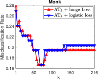
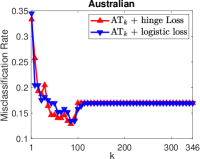
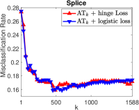
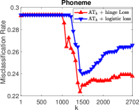
Figure 3: Plots of misclassification rate on testing set vs. $k$ on four datasets.

To further understand the behavior of MAT_k learning on individual datasets, we show plots of misclassification rate on testing set vs. $k$ for four representative datasets in Fig.3 (in which $C$ is fixed to $10^{2}$ and $k\in[1,n]$). As these plots show, on all four datasets, there is a clear range of $k$ value with better classification performance than the two extreme cases $k=1$ and $k=n$, corresponding to the maximum and average loss, respectively. To be more specific, when $k=1$, the potential noises and outliers will have the highest negative effects on the learned classifier and the related classification performance is very poor. As $k$ increases, the negative effects of noises and outliers will reduce and the classification performance becomes better, this is more significant on dataset Monk, Australian and Splice. However, if $k$ keeps increase, the classification performance may decrease (e.g., when $k=n$). This may because that as $k$ increases, more and more well classified samples will be included and the non-zero loss on these samples will have negative effects on the learned classifier (see our analysis in Section 2), especifically for dataset Monk, Australian and Phoneme.

Regression. Next, we report experimental results of linear regression on one synthetic dataset (Sinc) and three real datasets from chang2011libsvm , with a detailed description of these datasets given in Appendix. The standard square loss and absolute loss are adopted as individual losses. Note that average loss coupled with individual square loss is standard ridge regression model and average loss coupled with individual absolute loss reduces to $\nu$-SVR scholkopf2000new . We normalize the target output to $[0,1]$ and report their root mean square error (RMSE) in Table 2, with optimal $C$ and $k^{*}$ obtained by a grid search as in the case of classification (performance in terms of mean absolute square error (MAE) is given in Appendix). Similar to the classification cases, using the AT_k loss usually improves performance in comparison to the average loss or maximum loss.

	Square Loss			Absolute Loss
	Maximum	Average	AT${}_{k^{\ast}}$	Maximum	Average	AT${}_{k^{\ast}}$
Sinc	0.2790(0.0449)	0.1147(0.0060)	0.1139(0.0057)	0.1916(0.0771)	0.1188(0.0067)	0.1161(0.0060)
Housing	0.1531(0.0226)	0.1065(0.0132)	0.1050(0.0132)	0.1498(0.0125)	0.1097(0.0180)	0.1082(0.0189)
Abalone	0.1544(0.1012)	0.0800(0.0026)	0.0797(0.0026)	0.1243(0.0283)	0.0814(0.0029)	0.0811(0.0027)
Cpusmall	0.2895(0.0722)	0.1001(0.0035)	0.0998(0.0037)	0.2041(0.0933)	0.1170(0.0061)	0.1164(0.0062)

Table 2: Average RMSE on four datasets. The best results are shown in bold with results that are not significant different to the best results underlined.

5 Related Works

Most work on learning objectives focus on designing individual losses, and only a few are dedicated to new forms of aggregate losses. Recently, aggregate loss considering the order of training data have been proposed in curriculum learning bengio2009curriculum and self-paced learning kumar2010self ; spl2017 , which suggest to organize the training process in several passes and samples are included from easy to hard gradually. It is interesting to note that each pass of self-paced learning kumar2010self is equivalent to minimum the average of the $k$ smallest individual losses, i.e., ${1\over k}\sum_{i=n-k+1}^{n}\ell_{[i]}(f)$, which we term it as the average bottom-k loss in contrast to the average top-k losses in our case. In shalev2016minimizing , the pros and cons of the maximum loss and the average loss are compared, and the top-k loss, i.e., $\ell_{[k]}(f)$, is advocated as a remedy to the problem of both. However, unlike the AT_k loss, in general, neither the average bottom-k loss nor the top-k loss are convex functions with regards to the individual losses.

Minimizing top-$k$ errors has also been used in individual losses. For ranking problems, the work of rudin2009p ; usunier2009ranking describes a form of individual loss that gives more weights to the top examples in a ranked list. In multi-class classification, the top-$1$ loss is commonly used which causes penalties when the top-1 predicted class is not the same as the target class label crammer2001algorithmic . This has been further extended in lapin2015top ; lapin2016loss to the top-$k$ multi-class loss, in which for a class label that can take $m$ different values, the classifier is only penalized when the correct value does not show up in the top $k$ most confident predicted values. As an individual loss, these works are complementary to the AT_k loss and they can be combined to improve learning performance.

6 Discussion

In this work, we introduce the average top-$k$ (AT_k) loss as a new aggregate loss for supervised learning, which is the average over the $k$ largest individual losses over a training dataset. We show that the AT_k loss is a natural generalization of the two widely used aggregate losses, namely the average loss and the maximum loss, but can combine their advantages and mitigate their drawbacks to better adapt to different data distributions. We demonstrate that the AT_k loss can better protect small subsets of hard samples from being swamped by a large number of easy ones, especially for imbalanced problems. Furthermore, it remains a convex function over all individual losses, which can lead to convex optimization problems that can be solved effectively with conventional gradient-based methods. We provide an intuitive interpretation of the AT_k loss based on its equivalent effect on the continuous individual loss functions, suggesting that it can reduce the penalty on correctly classified data. We further study the theoretical aspects of AT_k loss on classification calibration and error bounds of minimum average top-$k$ learning for AT_k-SVM. We demonstrate the applicability of minimum average top-$k$ learning for binary classification and regression using synthetic and real datasets.

There are many interesting questions left unanswered regarding using the AT_k loss as learning objectives. Currently, we use conventional gradient-based algorithms for its optimization, but we are investigating special instantiations of MAT_k learning for which more efficient optimization methods can be developed. Furthermore, the AT_k loss can also be used for unsupervised learning problems (e.g., clustering), which is a focus of our subsequent study. It is also of practical importance to combine AT_k loss with other successful learning paradigms such as deep learning, and to apply it to large scale real life dataset. Lastly, it would be very interesting to derive error bounds of MAT_k with general individual loss functions.

7 Acknowledgments

This work was completed when the first author was a visiting student at SUNY Albany, supported by a scholarship from University of Chinese Academy of Sciences (UCAS). Siwei Lyu is supported by the National Science Foundation (NSF, Grant IIS-1537257) and Yiming Ying is supported by the Simons Foundation (#422504) and the 2016-2017 Presidential Innovation Fund for Research and Scholarship (PIFRS) program from SUNY Albany. This work is also partially supported by the National Science Foundation of China (NSFC, Grant 61620106003) for Bao-Gang Hu and Yanbo Fan.

Appendix A Proofs

A.1 Proofs of Lemma 1 and 2

Proof of Lemma 1

Notice that $\sum_{i=1}^{k}x_{[i]}$ is the solution of the following linear programming problem

$$\max_{\mathbf{p}}\ \mathbf{p}^{T}{\bf x},\ \ \text{s.t.}\ \ \mathbf{p}^{T}\mathbf{1}=k,\mathbf{0}\leq\mathbf{p}\leq\mathbf{1}.$$ (8)

The Lagrangian of this linear programming problem is

$$L(\mathbf{p},\mathbf{u},\mathbf{v},\lambda)=-\mathbf{p}^{T}{\bf x}-\mathbf{v}^{T}\mathbf{p}+\mathbf{u}^{T}(\mathbf{p}-\mathbf{1})+\lambda(\mathbf{p}^{T}\mathbf{1}-k),$$ (9)

where $\mathbf{u}\geq 0$, $\mathbf{v}\geq 0$ and t are Lagrangian multipliers. Taking its derivative w.r.t $\mathbf{p}$ and set it to be $\mathbf{0}$, we have $\mathbf{v}=\mathbf{u}-{\bf x}+\lambda\mathbf{1}$. Substituting this back into the Lagrangian to eliminate the primal variable, we obtain the dual problem of (8) as

$$\min_{\mathbf{u},\lambda}\ \mathbf{u}^{T}\mathbf{1}+k\lambda,\ \text{s.t.}\ \mathbf{u}\geq\mathbf{0},\mathbf{u}+\lambda\mathbf{1}-{\bf x}\geq\mathbf{0}.$$ (10)

This further means that

$$\sum_{i=1}^{k}x_{[i]}=\min_{\lambda}\Bigl{\{}k\lambda+\sum_{i=1}^{n}\left[x_{i}-\lambda\right]_{+}\Bigr{\}}.$$ (11)

The convexity of $\sum_{i=1}^{k}x_{[i]}$ follows directly from (11) and the fact that the partial minimum of a jointly convex function is convex. Furthermore, it is easy to see that $\lambda=x_{[k]}$ is always one optimal solution for (11), hence, for $x_{i}\geq 0,i=1,\cdots,n$, there holds

$$\sum_{i=1}^{k}x_{[i]}=\min_{\lambda\geq 0}\Bigl{\{}k\lambda+\sum_{i=1}^{n}\left[x_{i}-\lambda\right]_{+}\Bigr{\}}.$$ (12)

∎

Proof of Lemma 2

Denote $g(\ell)=\left[\left[a-\ell\right]_{+}-b\right]_{+}.$ For any $a\geq 0,b\geq 0$, we have $g(\ell)=0=\left[a-b-\ell\right]_{+}$ if $\ell\geq a$. In the Case of $\ell<a$, there holds $g(\ell)=\left[a-b-\ell\right]_{+}$. Thus $g(\ell)=\left[a-b-\ell\right]_{+}$ for any $a\geq 0,b\geq 0$.

∎

A.2 Proof of Theorem 1

Note that $\ell:\mathbb{R}\to\mathbb{R}^{+}$ is convex, differentiable at $0$ and $\ell^{\prime}(0)<0$ implies that $\ell(0)>0$. Hence, by normalization we can let $\ell(0)=1$. Indeed, the commonly used individual losses such as the least square loss $\ell(t)={(1-t)^{2}}$, the hinge loss $\ell(t)=(1-t)_{+}$, and the logistic loss $\ell(t)=\log_{2}(1+e^{-t})$ satisfy the conditions $\ell^{\prime}(0)<0$ and $\ell(0)=1$. The assumption in part (ii) of Theorem 1 implicitly assumes that ${\mathcal{E}}^{\ast}_{\ell}\leq 1$ because ${\mathcal{E}}^{\ast}_{\ell}\leq{\mathcal{E}}_{\ell}(0)=1$.

Since $(f^{\ast},\lambda^{\ast})$ is a minimizer, then, by choosing $f=0$ and $\lambda=\ell(0)=1$ there holds ${\mathbb{E}}[\ell(yf^{\ast}(x))-\lambda^{\ast})_{+}]+\nu\lambda^{\ast}\leq{\mathbb{E}}[(\ell(0)-\ell(0))_{+}]+\nu\ell(0)$ which implies that the minimizer $\lambda^{\ast}$ defined in (7) must satisfy $0\leq\lambda^{\ast}\leq\ell(0)=1$. This means that the minimization over $\lambda$ in (7) can be restricted to $0\leq\lambda\leq\ell(0)=1.$ Let $\beta=1-\lambda$ which implies that the minimization (7) is equivalent to the following

$$(f^{\ast},\beta^{\ast})=\arg\inf_{f,0\leq\beta\leq 1}\bigl{\{}{\mathbb{E}}[(\beta+\ell(yf(\mathbf{x}))-1)_{+}]-\nu\beta\bigr{\}}.$$ (13)

Let $(f^{\ast},\beta^{\ast})$ be the minimizer. We have, for any $f$ and choosing $\beta=\ell(0)=1$, that

$$-\nu\beta^{\ast}\leq\bigl{\{}{\mathbb{E}}[(\beta^{\ast}+\ell(yf^{\ast}(x))-1)_{+}]-\nu\beta^{\ast}\leq{\mathbb{E}}[(1+\ell(yf(\mathbf{x}))-1)_{+}]-\nu={\mathcal{E}}_{\ell}(f)-\nu.$$

This implies that $\nu\beta^{\ast}\geq\nu-{\mathcal{E}}_{\ell}(f)$. Since $f$ is arbitrary, $\beta^{\ast}\geq{\nu-{\mathcal{E}}^{\ast}_{\ell}\over\nu}>0$ if $\nu>{\mathcal{E}}^{\ast}_{\ell}$. Consequently, the above arguments show that $0\leq\lambda^{\ast}=1-\beta^{\ast}<1$ if $\nu>{\mathcal{E}}^{\ast}_{\ell}.$

Now observe that $f^{\ast}=\arg\inf_{f}\bigl{\{}{\mathbb{E}}[(\ell(yf(\mathbf{x}))-\lambda^{\ast})_{+}]+\nu\lambda^{\ast}\bigr{\}}=\arg\inf_{f}\bigl{\{}{\mathbb{E}}[(\ell(yf(\mathbf{x}))-\lambda^{\ast})_{+}]\bigr{\}}$. Define $\phi(t)=(\ell(t)-\lambda^{\ast})_{+}$. This means that $f^{\ast}=\arg\inf_{f}{\mathbb{E}}[\phi(yf(\mathbf{x}))]$ for standard classification. The result of Theorem 2 in bartlett2006convexity states that that the loss $\phi$ is classification calibrated if $\phi$ is differentiable at $0$ and $\phi^{\prime}(0)<0.$ Notice that $\lambda^{\ast}<\ell(0)=1$ as proved above, which implies that $\phi$ is differentiable at $0$ and $\phi^{\prime}(0)=\ell^{\prime}(0)<0$. This shows that $f^{\ast}$ has the same sign as the Bayes rule $\hbox{sign}(\Pr(y=1|\mathbf{x})-{1\over 2})$ if $\nu>{\mathcal{E}}^{\ast}_{\ell}.$ This completes the proof of the first part of the theorem.

We now move on to prove the proof of the second part of the theorem. To this end, observe that $\lambda^{\ast}=\mathop{\arg\!\inf}_{\lambda\geq 0}\bigl{\{}{\mathbb{E}}[\ell(yf^{\ast}(x))-\lambda)_{+}]+\nu\lambda\bigr{\}}.$ Assume that $\lambda^{\ast}=0$. Then, $f^{\ast}=f^{\ast}_{\ell}$ and choosing $f=0$ and $\lambda=1=\ell(0)$ in the objective function of (7) implies that $\nu={\mathbb{E}}[(\ell(0)-1)_{+}]+\nu\geq{\mathbb{E}}[\ell(yf^{\ast}(x))-\lambda^{\ast})_{+}]+\nu\lambda^{\ast}={\mathbb{E}}[\ell(yf^{\ast}_{\ell}(x))]\geq{\mathcal{R}}^{\ast}.$ Recall devroye2013probabilistic that the Bayes error ${\mathcal{R}}^{\ast}=\int_{\mathcal{X}}\min(\eta(\mathbf{x}),1-\eta(\mathbf{x}))\rho_{\mathcal{X}}(\mathbf{x}).$ This proves the Case $\lambda^{\ast}=0.$

Now it only suffices to prove the Case of $\lambda^{\ast}>0$. In this Case , by the first-order optimality condition, there exists a subgradient of ${\mathbb{E}}[\ell(yf^{\ast}(x))-\lambda)_{+}]+\nu\lambda$ of the variable $\lambda$ at $\lambda^{\ast}$ equals to zero. This implies that ${\mathbb{E}}[h(x,y)]+\nu=0,$ where $h(x,y)$ is some subgradient of $(\ell(yf^{\ast}(x))-\lambda)_{+}$ with respect to $\lambda$ at $\lambda^{\ast}$. Notice that $h(x,y)\leq-\mathbb{I}_{\ell(yf^{\ast}(x))>\lambda^{\ast}}.$ Consequently, $\nu\geq{\mathbb{E}}[\mathbb{I}_{\ell(yf^{\ast}(x))>\lambda^{\ast}}]\geq{\mathbb{E}}[\mathbb{I}_{\ell(yf^{\ast}(x))>\ell(0)}]$ since $\lambda^{\ast}\leq\ell(0)$ as proved in part (i). Since we assume that $\ell$ is monotonically decreasing, $\ell(yf^{\ast}(x))>\ell(0)$ is equivalent to $yf^{\ast}(x)<0.$ The calibration of AT_k models (i.e. $f^{\ast}$ has the sign as the Bayes rule) implies that $yf^{\ast}(x)<0$ is equivalent to $y(2\eta(x)-1)<0.$ Putting the above arguments together, we conclude that $\nu\geq{\mathbb{E}}[\mathbb{I}_{y(2\eta(x)-1)<0}]=\int_{\eta(x)\neq{1/2}}\min(\eta(x),1-\eta(x)).$ This completes the proof of the theorem.

A.3 Proof of Theorem 2

Steinwart steinwart2003optimal derived the bounds for the excess misclassification error for $\nu$-SVM under the assumption that the kernel is universal, i.e., the RKHS is dense in the space of continuous functions $\mathcal{C}(\mathcal{X})$ under the uniform norm $\|\cdot\|_{\infty}$ (See steinwart2008support for more details). The proof there depends on Urysohn’s lemma in topology which states any two disjoint closed subsets can be separated by a continuous function. In contrast, our result holds true without the assumption of universal kernels.

To prove Theorem 2, we need some technical lemmas. We say the function $F:\displaystyle\displaystyle\prod_{k=1}^{m}\Omega_{k}\rightarrow\mathbb{R}$ has bounded differences $\{c_{k}\}_{k=1}^{m}$ if, for all $1\leq k\leq m$,

$$\max_{z_{1},\cdots,z_{k},z^{\prime}_{k}\cdots,z_{m}}|F(z_{1},\cdots,z_{k-1},z_{k},z_{k+1},\cdots,z_{m})-F(z_{1},\cdots,z_{k-1},z^{\prime}_{k},z_{k+1},\cdots,z_{m})|\leq c_{k}.$$

Lemma 3.

(McDiarmid’s inequality mcdiarmid1989method) Suppose $f:\displaystyle\displaystyle\prod_{k=1}^{m}\Omega_{k}\rightarrow\mathbb{R}$ has bounded differences $\{c_{k}\}_{k=1}^{m}$ then , for all $\epsilon>0$, there holds

$$\Pr\biggl{\{}F({\bf z})-\mathbb{E}[F({\bf z})]\geq\epsilon\biggr{\}}\leq e^{-\frac{2\epsilon^{2}}{\sum_{k=1}^{m}c_{k}^{2}}}.$$

We need to use the the Rademacher average and its contraction property bartlett2002rademacher,meir-zhang.

Definition 1.

Let $\mu$ be a probability measure on $\Omega$ and $F$ be a class of uniformly bounded functions. For every integer $m$, the Rademacher average over a set of functions F on Ω

$$R_{m}(F):={\mathbb{E}}_{\mu}{\mathbb{E}}_{\epsilon}\Big{\{}{1\over{{m}}}\displaystyle\sup_{f\in F}\Big{|}\displaystyle\sum_{i=1}^{m}\sigma_{i}f(z_{i})\Big{|}\Big{\}}$$

where $\{z_{i}\}_{i=1}^{m}$ are independent random variables distributed according to $\mu$ and $\{\sigma_{i}\}_{i=1}^{m}$ are independent Rademacher random variables, i.e., $\Pr(\sigma_{i}=+1)=\Pr(\sigma_{i}=-1)=1/2$.

Lemma 4.

Let $F$ be a class of uniformly bounded real-valued functions on $(\Omega,\mu)$ and $m\in\mathbb{N}$. If for each $i\in\{1,\ldots,m\}$, $\Psi_{i}:\mathbb{R}\to\mathbb{R}$ is a function with a Lipschitz constant $c_{i}$, then for any $\{x_{i}\}_{i=1}^{m}$,

$${\mathbb{E}}_{\epsilon}\Big{(}\displaystyle\sup_{f\in F}\big{|}\displaystyle\sum_{i=1}^{m}\epsilon_{i}\Psi_{i}(f(x_{i}))\big{|}\Big{)}\leq 2{\mathbb{E}}_{\epsilon}\Big{(}\displaystyle\sup_{f\in F}\Big{|}\displaystyle\sum_{i=1}^{m}c_{i}\epsilon_{i}f(x_{i})\big{|}\Big{)}.$$ (14)

Using the standard techniques involving Rademacher averages bartlett2002rademacher, one can get the following estimation. For completeness, we give a self-contained proof. Let the empirical error related to the hinge loss be denoted by ${\mathcal{E}}_{h,{\bf z}}(f)={1\over n}\sum_{i=1}^{n}(1-yf(\mathbf{x}_{i}))_{+}.$

Lemma 5.

For any $\varepsilon>0$, there holds

$$\Pr\biggl{\{}\displaystyle\sup_{\|f\|_{K}\leq R}{\mathcal{E}}_{h}(f)-{\mathcal{E}}_{h,{\bf z}}(f)\geq\varepsilon+{2\kappa R\over\sqrt{n}}\biggr{\}}\leq e^{-{2n\varepsilon^{2}\over(1+\kappa R)^{2}}}.$$

Proof.

Let $F(z)=\displaystyle\sup_{\|f\|_{K}\leq R}[{\mathcal{E}}_{h}(f)-{\mathcal{E}}_{h,{\bf z}}(f)].$ Observe, for any $x,y$, that $(1-yf(x))_{+}\leq 1+|f(x)|\leq 1+|\langle K_{x},f\rangle_{K}|\leq 1+\|f\|{\langle K_{x},K_{x}\rangle_{K}}^{1\over 2}=1+\|f\|_{K}\sqrt{K(x,x)}\leq\kappa R.$ Then, one can easily get that the bounded differences are $c_{k}={1+\kappa R\over n}$ for any $1\leq k\leq n.$ By the McDiarmid inequality, we have

$${\Pr}\biggl{\{}\displaystyle\sup_{\|f\|_{K}\leq R}[{\mathcal{E}}_{h}(f)-{\mathcal{E}}_{h,{\bf z}}(f)]\geq{\mathbb{E}}_{\bf z}\displaystyle\sup_{\|f\|_{K}\leq R}[{\mathcal{E}}_{h}(f)-{\mathcal{E}}_{h,{\bf z}}(f)]+\varepsilon\biggr{\}}\geq\exp\Bigr{\{}-{2n\varepsilon^{2}\over(1+\kappa R)^{2}}\Bigl{\}}.$$

Let ${\bf z}^{\prime}=\{z_{1}^{\prime},z_{2}^{\prime},\ldots,z_{n}^{\prime}\}$ be i.i.d. copies of ${\bf z}.$ Then,

$${\mathbb{E}}_{\bf z}\displaystyle\sup_{\|f\|_{K}\leq R}[{\mathcal{E}}_{h}(f)-{\mathcal{E}}_{h,{\bf z}}(f)]={\mathbb{E}}_{\bf z}[\displaystyle\sup_{\|f\|_{K}\leq R}[{\mathbb{E}}_{{\bf z}^{\prime}}({\mathcal{E}}_{{\bf z}^{\prime}}(f))-{\mathcal{E}}_{h,{\bf z}}(f)]\leq{\mathbb{E}}_{\bf z}{\mathbb{E}}_{{\bf z}^{\prime}}\displaystyle\sup_{\|f\|_{K}\leq R}[{\mathcal{E}}_{{\bf z}^{\prime}}(f)-{\mathcal{E}}_{h,{\bf z}}(f)].$$

By standard symmetrization techniques bartlett2002rademacher, for any Rademacher variables $\{\sigma_{i}:i=1,\ldots,n\}$, we have that

$${\mathbb{E}}_{\bf z}{\mathbb{E}}_{{\bf z}^{\prime}}\displaystyle\sup_{\|f\|_{K}\leq R}[{\mathcal{E}}_{h}(f)-{\mathcal{E}}_{h,{\bf z}}(f)]={\mathbb{E}}_{\bf z}{\mathbb{E}}_{{\bf z}^{\prime}}{\mathbb{E}}_{\sigma}\displaystyle\sup_{\|f\|_{K}\leq R}[{1\over n}\displaystyle\sum_{i=1}^{n}\sigma_{i}((1-y^{\prime}_{i}f(x^{\prime}_{i}))_{+}-(1-y_{i}f(x_{i}))_{+})]$$

$$=2{\mathbb{E}}_{\bf z}{\mathbb{E}}_{\sigma}\displaystyle\sup_{\|f\|_{K}\leq R}\bigl{[}{1\over n}\displaystyle\sum_{i=1}^{n}\sigma_{i}(1-y_{i}f(x_{i}))_{+}\bigr{]}\leq 2{\mathbb{E}}_{\bf z}{\mathbb{E}}_{\sigma}\displaystyle\sup_{\|f\|_{K}\leq R}{1\over n}\Big{|}\displaystyle\sum_{i=1}^{n}\sigma_{i}(1-y_{i}f(x_{i}))_{+}\Big{|}.$$

Let $\Phi_{i}(t)=(1-y_{i}t)_{+}$ which has Lipschitz constant $1$. By the contraction property of Rademacher averages,

$${\mathbb{E}}_{\sigma}\displaystyle\sup_{\|f\|_{K}\leq R}{1\over n}\Big{|}\displaystyle\sum_{i=1}^{n}\sigma_{i}(1-y_{i}f(x_{i}))_{+}\Big{|} \leq{\mathbb{E}}_{\sigma}\displaystyle\sup_{\|f\|_{K}\leq R}{1\over n}\Big{|}\displaystyle\sum_{i=1}^{n}\sigma_{i}f(x_{i})\Big{|}={\mathbb{E}}_{\sigma}\displaystyle\sup_{\|f\|_{K}\leq R}\Big{|}\langle{1\over n}\displaystyle\sum_{i=1}^{n}\sigma_{i}K_{x_{i}},f\rangle\Big{|}$$

$$\leq{\mathbb{E}}_{\sigma}\displaystyle\sup_{\|f\|_{K}\leq R}\|{1\over n}\displaystyle\sum_{i=1}^{n}\sigma_{i}K_{x_{i}}\|_{K}\|f\|_{K}=R\>{\mathbb{E}}_{\sigma}\Big{[}\|{1\over n}\displaystyle\sum_{i=1}^{n}\sigma_{i}K_{x_{i}}\|_{K}\Big{]}$$

$$\leq R\>\Big{[}{\mathbb{E}}_{\sigma}\|{1\over n}\displaystyle\sum_{i=1}^{n}\sigma_{i}K_{x_{i}}\|^{2}_{K}\Big{]}^{1\over 2}\leq{R\over n}\Big{[}\displaystyle\sum_{i=1}^{n}K(x_{i},x_{i})\Big{]}^{1\over 2}\leq{\kappa R\over\sqrt{n}}.$$

Putting all the above estimations together yields the desired result. This completes the proof of the lemma. ∎

We also need the Höeffding’s inequality stated as follows.

Lemma 6.

Let $\xi$ be a random variable and, for any $i\in[m]$, $a_{i}\leq\xi\leq b_{i}.$ Then, for any $\varepsilon>0$, there holds

$${\Pr}\biggl{\{}{1\over m}\displaystyle\sum_{i=1}^{m}\xi_{i}-E\xi\geq\epsilon\biggr{\}}\leq\exp\biggl{\{}-{m\epsilon^{2}\over{2M^{2}}}\biggr{\}}.$$

To prove the main theorem, we need to establish a lower bound for $\rho_{\bf z}.$ Denote $\kappa=\sup_{x\in\mathcal{X}}\sqrt{K(x,x)}.$

Lemma 7.

For $\mu\in(0,1-{\mathcal{E}}_{h}(f_{\mathcal{H}}))$, let $\lceil n({\mathcal{E}}_{h}(f_{\mathcal{H}})+\mu)\rceil\leq k\leq n$, then we have

$$\Pr\biggl{\{}{\bf z}\in\mathcal{Z}^{n}:{\|f_{\bf z}\|_{K}\over\rho_{\bf z}}\leq{2k\over n}\max\Bigl{(}\sqrt{2C\over\mu},{2\|f_{\mathcal{H}}\|_{K}\over\mu}\Bigr{)}\biggr{\}}\geq 1-\exp\Bigl{\{}-{n\mu^{2}\over 2(1+\kappa\|f_{\mathcal{H}}\|_{K})^{2}}\Bigr{\}}.$$

Proof.

Since $(f_{\bf z},\rho_{\bf z})$ is a minimizer of formulation (6), for any $0<\rho\leq 1$ there holds

$${1\over n}\sum_{i=1}^{n}(\rho_{\bf z}-y_{i}f_{\bf z}(x_{i}))_{+}-{k\over n}\rho_{\bf z}+{1\over 2C}\|f_{\bf z}\|^{2}_{K} \leq{1\over n}\displaystyle\sum^{n}(\rho-y_{i}\rho f_{\mathcal{H}}(x_{i}))_{+}-{k\over n}\rho+{1\over 2C}\|\rho f_{\mathcal{H}}\|^{2}_{K}$$

$$=\rho{\mathcal{E}}_{h,{\bf z}}(f_{\mathcal{H}})-{k\over n}\rho+\frac{\rho^{2}}{2C}\|f_{\mathcal{H}}\|^{2}_{K}.$$ (15)

This implies, for any $0<\rho\leq 1$, that

$${k\over n}\rho_{\bf z}\geq-\rho{\mathcal{E}}_{h,{\bf z}}(f_{\mathcal{H}})+{k\over n}\rho-\frac{\rho^{2}}{2C}\|f_{\mathcal{H}}\|^{2}_{K}.$$

Applying the Hoeffding inequality (Lemma 6) yields that

$$\Pr\Bigl{\{}{\mathcal{E}}_{h,{\bf z}}(f_{\mathcal{H}})-{\mathcal{E}}_{h}(f_{\mathcal{H}})\leq{\mu\over 2}\Bigr{\}}\leq 1-\exp\Bigl{\{}-{n\mu^{2}\over 2(1+\kappa\|f_{\mathcal{H}}\|_{K})^{2}}\Bigr{\}}.$$ (16)

Then, on the event  $\mathcal{U}=\bigl{\{}{\bf z}\in\mathcal{Z}^{n}:{\mathcal{E}}_{h,{\bf z}}(f_{\mathcal{H}})-{\mathcal{E}}_{h}(f_{\mathcal{H}})\leq{\mu\over 2}\bigr{\}},$ we have $-\rho{\mathcal{E}}_{h,{\bf z}}(f_{\mathcal{H}})+{k\over n}\rho-\frac{\rho^{2}}{2C}\|f_{\mathcal{H}}\|^{2}_{K}\geq{\rho({k\over n}-{\mathcal{E}}(f_{\mathcal{H}})-{\mu\over 2})}-\frac{\rho^{2}}{2C}\|f_{\mathcal{H}}\|^{2}_{K}\geq\rho{\mu\over 2}-\frac{\rho^{2}}{2C}\|f_{\mathcal{H}}\|^{2}_{K}.$ Define $g(\rho)={\rho\mu\over 2}-\frac{\rho^{2}}{2C}\|f_{\mathcal{H}}\|^{2}_{K}.$ It is easy to observe that

$$\max_{0<\rho\leq 1}g(\rho)\geq\left\{\begin{array}[]{ll}{C\mu^{2}\over 8\|f_{\mathcal{H}}\|^{2}_{K}},&C\mu\leq 2\|f_{\mathcal{H}}\|_{K}^{2},\\ {\mu\over 4},&C\mu>2\|f_{\mathcal{H}}\|_{K}^{2}.\end{array}\right.$$

Consequently, on the event $\mathcal{U}$, there holds

$$\rho_{\bf z}\geq{n\over k}\displaystyle\max_{0<\rho\leq 1}g(\rho)\geq{n\over k}\min\bigl{(}{\mu\over 4},{C\mu^{2}\over 8\|f_{\mathcal{H}}\|_{K}^{2}}\bigr{)}.$$ (17)

By choosing $\rho=0$ in (15), there holds ${\|f_{\bf z}\|_{K}^{2}\over\rho_{\bf z}}\leq{2Ck\over n}$. Combining these estimation together, on the event $\mathcal{U}$ there holds

$${\|f_{\bf z}\|_{K}\over\rho_{\bf z}}\leq\sqrt{\|f_{\bf z}\|_{K}^{2}\over\rho_{\bf z}}\sqrt{1\over\rho_{\bf z}}\leq{2k\over n}\max\biggl{(}\sqrt{2C\over\mu},{2\|f_{\mathcal{H}}\|_{K}\over\mu}\biggr{)}.$$

This completes the proof of the lemma. ∎

With all the above technical lemmas, we are ready to prove Theorem 2.

Proof of Theorem 2. We will use the relationship between the excess misclassification error and generalization error zhang2004statistical, i.e.  for any $f:\mathcal{X}\to\mathbb{R}$, there holds

$${\mathcal{R}}(\hbox{sign}(f))-{\mathcal{R}}(f_{c})\leq{\mathcal{E}}_{h}(f)-{\mathcal{E}}_{h}(f_{c}).$$ (18)

Let $\mathcal{U}_{1}$ be the event such that the inequality in Lemma 7 is true, i.e.  $\mathcal{U}_{1}=\bigl{\{}{\bf z}\in\mathcal{Z}^{n}:{\|f_{\bf z}\|_{K}\over\rho_{\bf z}}\leq{2k\over n}\max\bigl{(}\sqrt{2C\over\mu},{2\|f_{\mathcal{H}}\|_{K}\over\mu}\bigr{)}\bigr{\}}.$ On the event $\mathcal{U}_{1}$, noting that $0<\mu\leq 1$ we have that ${\|f_{\bf z}\|_{K}\over\rho_{\bf z}}\leq R_{C,\mu}:={2\sqrt{2C}+4\|f_{\mathcal{H}}\|_{K}\over\mu}.$

Now considering the sample ${\bf z}\in\mathcal{U}_{1},$ using (18) we have

$${\cal R}(\hbox{sign}(f_{\bf z}))-{\cal R}(f_{c})\leq{\mathcal{E}}_{h}\bigl{(}{f_{\bf z}\over\rho_{\bf z}}\bigr{)}-{\mathcal{E}}(f_{c})\leq{\mathcal{E}}_{h}\bigl{(}\frac{f_{\bf z}}{\rho_{\bf z}}\bigr{)}-{\mathcal{E}}_{h,\bf z}(\frac{f_{\bf z}}{\rho_{\bf z}})+{\mathcal{E}}_{h,\bf z}(\frac{f_{\bf z}}{\rho_{\bf z}})-{\mathcal{E}}(f_{c})$$ (19)

By the definition of the minimizer $(\rho_{\bf z},f_{\bf z})$, there holds ${1\over n}\sum_{i=1}^{n}(\rho_{\bf z}-y_{i}f_{\bf z}(x_{i}))_{+}-{k\over n}\rho_{\bf z}+{1\over 2C}\|f_{\bf z}\|^{2}_{K}\leq 0$ which means that ${1\over n}\sum_{i=1}^{n}(\rho_{\bf z}-y_{i}f_{\bf z}(x_{i}))_{+}\leq{k\over n}\rho_{\bf z}.$ Equivalently, ${\mathcal{E}}_{h,{\bf z}}\bigl{(}{f_{\bf z}\over\rho_{\bf z}}\bigr{)}\leq{k\over n}$ on the event $\mathcal{U}_{1}$. This combines with (19) implies, on the event $\mathcal{U}_{1}$, that

$${\cal R}(\hbox{sign}(f_{\bf z}))-{\cal R}(f_{c}) \leq{\mathcal{E}}_{h}\bigl{(}\frac{f_{\bf z}}{\rho_{\bf z}}\bigr{)}-{\mathcal{E}}_{h,\bf z}(\frac{f_{\bf z}}{\rho_{\bf z}})+({k\over n}-{\mathcal{E}}_{h}(f_{\mathcal{H}}))+{\mathcal{E}}_{h}(f_{\mathcal{H}})-{\mathcal{E}}(f_{c})$$

$$\leq\displaystyle\sup_{\|f\|_{K}\leq R_{C,\mu}}\Bigl{[}{\mathcal{E}}_{h}\bigl{(}f\bigr{)}-{\mathcal{E}}_{h,{\bf z}}(f)\Bigr{]}+({k\over n}-{\mathcal{E}}_{h}(f_{\mathcal{H}}))+\inf_{f\in\mathcal{H}_{K}}{\mathcal{E}}_{h}(f)-{\mathcal{E}}_{h}(f_{c})$$

$$\leq\displaystyle\sup_{\|f\|_{K}\leq R_{C,\mu}}\Bigl{[}{\mathcal{E}}_{h}\bigl{(}f\bigr{)}-{\mathcal{E}}_{h,{\bf z}}(f)\Bigr{]}+({k\over n}-{\mathcal{E}}_{h}(f_{\mathcal{H}}))+{\mathcal{A}}(\mathcal{H}_{K})$$

$$\leq\displaystyle\sup_{\|f\|_{K}\leq R_{C,\mu}}\Bigl{[}{\mathcal{E}}_{h}\bigl{(}f\bigr{)}-{\mathcal{E}}_{h,{\bf z}}(f)\Bigr{]}+\mu+{1\over n}+{\mathcal{A}}(\mathcal{H}_{K}),$$

where the last inequality follows from the fact, by the definition $k=k(n)=\lceil n({\mathcal{E}}_{h}(f_{\mathcal{H}})+\mu)\rceil$, that ${\mathcal{E}}_{h}(f_{\mathcal{H}})+\mu\leq{k\over n}\leq{\mathcal{E}}_{h}(f_{\mathcal{H}})+\mu+{1\over n}.$ Therefore,

$$\Pr\biggl{\{}{\bf z}\in\mathcal{Z}^{n}:{\cal R}(\hbox{sign}(f_{\bf z}))-{\cal R}(f_{c})\geq{\mu}+{1\over n}+{\mathcal{A}}(\mathcal{H})+\varepsilon+{2\kappa R_{C,\mu}\over\sqrt{n}}\biggr{\}}$$

$$\leq\Pr(\mathcal{U}_{1}^{c})+\Pr\biggl{\{}{\bf z}\in\mathcal{U}_{1}:\displaystyle\sup_{\|f\|_{K}\leq R_{C,\mu}}\bigl{[}{\mathcal{E}}_{h}\bigl{(}f\bigr{)}-{\mathcal{E}}_{h,{\bf z}}(f)\bigr{]}\geq\varepsilon+{2\kappa R_{C,\mu}\over\sqrt{n}}\biggr{\}}$$

$$\leq\exp\biggl{(}-{n\mu^{2}\over 2(1+\kappa\|f_{\mathcal{H}}\|_{K})^{2}}\biggr{)}+\Pr\biggl{\{}{\bf z}:\displaystyle\sup_{\|f\|_{K}\leq R_{C,\mu}}\bigl{[}{\mathcal{E}}_{h}\bigl{(}f\bigr{)}-{\mathcal{E}}_{h,{\bf z}}(f)\bigr{]}\geq\varepsilon+{2\kappa R_{C,\mu}\over\sqrt{n}}\biggr{\}}$$

$$\leq\exp\biggl{(}-{n\mu^{2}\over 2(1+\kappa\|f_{\mathcal{H}}\|_{K})^{2}}\biggr{)}+\exp\biggl{(}-{2n\varepsilon^{2}\over(1+\kappa R_{C,\mu})^{2}}\biggr{)}$$

$$\leq 2\exp\biggl{(}-{n\varepsilon^{2}\mu^{2}\over(1+2\kappa\sqrt{2C}+4\kappa\|f_{\mathcal{H}}\|_{K})^{2}}\biggr{)}.$$

Here, the second to last inequality follows from Lemma 5 which is the standard estimation for Rademacher averages bartlett2002rademacher. ∎

Appendix B Examples of AT_k loss coupled with different individual losses

The proposed AT_k loss is quite general and can be combined with different existing individual losses. An interesting phenomenon is that AT_k with hinge loss and absolute loss have a close relations to the well-known $\nu$-SVM and $\nu$-SVR that proposed in scholkopf2000new , respectively. Specifically, we have

Proposition 1.

Under conditions $C=1$ and $K(\mathbf{x}_{i},\mathbf{x}_{i})\leq 1$ for any $i$, AT_k-SVM (6) reduces to $\nu$-SVM with $\nu={k\over n}$.

Proof.

Recall scholkopf2000new that the primal problem of the $\nu$-SVM without the bias term $b$ is formulated by

$$\min_{f\in\mathcal{H}_{K},\rho\geq 0}{1\over n}\sum_{i=1}^{n}\left[\rho-y_{i}f(\mathbf{x}_{i})\right]_{+}-\nu\rho+{1\over 2}\|f\|_{K}^{2},$$ (20)

where $\nu\in[0,1]$ is a scalar. Its dual is given by

$$\left\{\begin{array}[]{cl}\min_{\alpha}&{1\over 2}\displaystyle\sum_{i,j=1}^{n}\alpha_{i}\alpha_{j}y_{i}y_{j}K(x_{i},x_{j})\\ \hbox{s.t.}&0\leq\alpha_{i}\leq{1\over n},\forall i=1,2,\ldots,n\\ &\displaystyle\sum_{i=1}^{n}\alpha_{i}\geq\nu.\end{array}\right.$$

The KKT conditions implies, for any optimal solution $\alpha^{\ast}$ of the dual and any optimal solution $(f_{\bf z},\rho_{\bf z})$ of the primal, there holds, for the support vectors $\mathbf{x}_{i}$ with $0<\alpha^{\ast}_{i}<{1\over n}$, that $\rho_{\bf z}=y_{i}\sum_{j=1}^{n}\alpha^{\ast}_{j}y_{j}K(\mathbf{x}_{i},\mathbf{x}_{j})$. If one assumes that $K(\mathbf{x}_{i},\mathbf{x}_{i})\leq 1$ for all $i$, then $|K(x_{i},x_{j})|=|\langle K_{\mathbf{x}_{i}},K_{\mathbf{x}_{j}}\rangle_{K}|\leq\sqrt{K(\mathbf{x}_{i},\mathbf{x}_{i})}\sqrt{K(\mathbf{x}_{j},\mathbf{x}_{j})}\leq 1$. Therefore,

$$\rho_{\bf z}\leq|y_{i}\sum_{j=1}^{n}\alpha^{\ast}_{j}y_{j}K(\mathbf{x}_{i},\mathbf{x}_{j})|\leq\sum_{j=1}^{n}\alpha^{\ast}_{j}\leq 1,$$

where the last inequality follows from the fact that $\alpha_{j}\leq{1\over n}$ for all $j.$ Consequently, in the minimization of (20) we can restrict to $\rho\leq 1$ which implies that the AT_k-SVM (6) with $C=1$ is reduced to $\nu$-SVM with $\nu={k\over n}.$ ∎

Besides, the dual formulation of AT_k-SVM (6) can be easily derived as

$$\left\{\begin{array}[]{cl}\min_{\alpha}&{1\over 2}\displaystyle\sum_{i,j=1}^{n}\alpha_{i}\alpha_{j}y_{i}y_{j}K(x_{i},x_{j})-\displaystyle\sum_{i=1}^{n}\alpha_{i}\\ \hbox{s.t.}&0\leq\alpha_{i}\leq{C\over n},\forall i=1,2,\ldots,n\\ &\displaystyle\sum_{i=1}^{n}\alpha_{i}\leq{Ck\over n}.\end{array}\right.$$

This leads to a convex quadratic programming problem for AT_k-SVM and can be solved efficiently.

Proposition 2.

MAT_k model (3) coupled with absolute loss in the RKHS setting becomes $\nu$-SVR with $\nu={k\over n}$.

Proof.

Recall scholkopf2000new that the primal problem of the $\nu$-SVR without the bias term $b$ in RKHS is formulated by

$$\min_{\mathbf{w},\lambda\geq 0}{1\over n}\sum_{i=1}^{n}\left[|y_{i}-f(x_{i})|-\lambda\right]_{+}+\nu\lambda+{1\over 2C}\|f\|_{K}^{2},$$ (21)

where $\nu\in[0,1]$ is a scalar. It is easy to see in the setting of RKHS that, with individual absolute loss (i.e., $\ell(f(\mathbf{x}_{i}),y_{i})=|y_{i}-f(\mathbf{x}_{i})|$) and $\Omega(\mathbf{w})={1\over 2C}\|f\|_{K}^{2}$, MAT_k model (3) becomes

$$\min_{\mathbf{w},\lambda\geq 0}{1\over n}\sum_{i=1}^{n}\left[|y_{i}-f(\mathbf{x}_{i})|-\lambda\right]_{+}+{k\over n}\lambda+{1\over 2C}\|f\|_{K}^{2},$$ (22)

We name model (22) as AT_k-SVR for brevity. It is straightforward that AT_k-SVR is exactly the $\nu$-SVR with $\nu={k\over n}$.

The above propositions provide new perspectives to understand the success of $\nu$-SVM and $\nu$-SVR. That is, through “shifting down” the original individual hinge loss and absolute loss and truncating them at zero, the penalty of correctly classified samples that are “far enough” from classification boundary in classification and the penalty of samples that are “close enough” to the regression tube in regression will be zero, which enables the model to put more effort to misclassified samples or samples that are “too far” to the regression tube. Besides, the good properties of $\nu$ in $\nu$-SVM and $\nu$-SVR that derived in scholkopf2000new can be extended to $k$ in AT_k-SVM and AT_k-SVR directly. For example, for AT_k-SVM with conditions $C=1$ and $K(\mathbf{x}_{i},\mathbf{x}_{i})\leq 1$ and AT_k-SVR, $k$ is a lower bound on the number of support vectors and is an upper bound on the number of margin errors. Due to its directness, we refer to scholkopf2000new for their proofs. This can also help us select $k$ in AT_k-SVM and AT_k-SVR.

∎

Appendix C Toy examples for effects of different aggregate losses

We illustrate the behaviors of different aggregate losses using binary classification on 2D synthetic data examples. We generate six different datasets (Fig. 4). Each dataset consists of 200 samples sampled from Gaussian distributions with distinct centers and variances. We use linear classifier and consider different aggregate losses combined with individual logistic loss and individual hinge loss. The learned linear classifiers and the misclassification rate of AT_k vs. $k$ are shown in Fig. 4. The left panel in Fig. 4 (i.e., (a1-a6) and (b1-b6)) refers to the results of aggregate losses combined with individual logistic loss and the right panel (i.e., (c1-c6) and (d1-d6)) refers to the results of aggregate losses combined with individual hinge loss.

Case 1. The first row in Fig. 4 represents an ideal situation where there is no outliers and the $+$ samples and $-$ samples are well distributed and linear separable. In this Case , all aggregate losses with both logistic loss and hinge loss can get perfect classification results. This is also verified in Fig. 4 (b1) and Fig. 4 (d1) that the misclassification rate is zero for AT_k with all $k$.

Case 2. In the second row, there exists an outlier in the $+$ class (shown as an enlarged $\times$). We can see that the maximum loss is very sensitive to outliers and its classification boundary in Fig. 4 (a2) and Fig. 4 (c2) are largely influenced by this outlier. Seen from Fig. 4 (b2) and Fig. 4 (d2), AT_k loss is more robust with larger $k$ and achieves better classification results when $k\geq 3$.

Case 3. In the third row, there is no outliers and the $+$ samples and $-$ samples are still linear separable. However, the $+$ samples clearly has two distributions (typical distribution and rare distribution). Seen from Fig. 4 (a3) and Fig. 4 (c3), the linear classifiers learned from average loss sacrifice some $+$ samples from rare distribution even though the data are separable. This is because that the individual logistic loss has non-zero penalty for correctly classified samples and individual hinge loss has non-zero penalty for correctly classified samples with margin less than 1. Hence samples that are “too close” to the classification boundary (samples from rare distributions in this example) are sacrificed to accommodate reducing the average loss over the whole datasets. Besides, average with hinge loss achieves better results than that with logistic loss, this may because that for correctly classified samples with margin larger than 1, the penalty caused by hinge loss is zero while that caused by logistic loss is still non-zeros. Hence this part of samples still has “negative” effect to the learned classification boundary of average with logistic loss. By “shifting down” and truncating, AT_k loss with proper $k$ (e.g., $k\in[1,18]$ for logistic loss and $k\in[1,50]$ for hinge loss) can better fit this data, as is shown in Fig. 4 (b3) and Fig. 4 (d3).

Case 4. The plots in the fourth row refers to a more complicated situation where there are both multi-modal distributions and outliers. Obviously, neither maximum loss (due to the outlier) nor average loss (due to the multi-modal distributions) can fit this data very well. Seen from Fig. 4 (b4) and Fig. 4 (d4), there exists a proper region of $k$ (i.e., $k\in[4,24]$ for logistic loss and $k\in[3,62]$ for hinge loss) that can yield much better classification results. We also report the linear classifier learned from AT_k=10 for better understanding. Seen from Fig. 4 (a4) and Fig. 4 (c4), the classification boundary of AT_k=10 is closer to the optimal Bayes linear classifier than that of maximum and average.

Case 5. The fifth row shows an imbalance scenario where the $-$ samples are far less that the $+$ ones. The $+$ samples and $-$ samples are linear separable. We can see from Fig. 4 (a5) that the average loss with individual logistic loss sacrifices all $-$ samples to obtain a small loss over the whole dataset. While the average loss with individual hinge loss obtains better results, it still sacrifices half of the $-$ samples, as is shown in Fig. 4 (c5). In contrast, AT_k loss can better fit this distributions and achieves better classification results with $k\in[1,25]$ for logistic loss and $k\in[1,135]$ for hinge loss.

Case 6. The sixth row shows an imbalanced data with one outlier. Comparing to the results in the fifth row, the performance of maximum loss decreases due to the outlier. The performance of average loss with hinge loss also decreases. Seen from Fig. 4 (b6) and Fig. 4 (d6), AT_k loss with $k\in[2,12]$ for logistic loss and $k\in[3,59]$ for hinge loss can better fit this data and achieve better classification results.

Though very simple, these synthetic datasets reveal some properties of the maximum loss and average loss intuitively. That is, while maximum loss performs very well for separable data, it it very sensitive to outliers. Meanwhile, average loss is more robust to outliers than maximum loss, however, it may sacrifices some correctly classified samples that are “too close” to the classification boundary, especially in imbalanced or multi-modal data distributions. As the distributions of datasets from real applications can be very complicated and outliers are unavoidable, it is interesting and helpful to add an extra freedom $k$ to better fitting different data distributions.

Binary Classification										Regression
Dataset	$c$	$n$	$d$	$IR$	Dataset	$c$	$n$	$d$	$IR$	Dataset	$n$	$d$
Monk	2	432	6	1.12	Spambase	2	4601	57	1.54	Sinc	1000	10
Australian	2	690	14	1.25	German	2	1000	24	2.33	Housing	506	13
Madelon	2	2600	500	1.0	Titanic	2	2201	3	2.10	Abalone	4177	8
Splice	2	3175	60	1.08	Phoneme	2	5404	5	2.41	Cpusmall	8192	12

Table 3: Statistical information of each dataset, where $c,n,d$ are the number of classes, samples and features, respectively. IR is the class ratio.

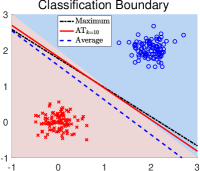
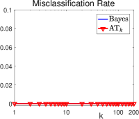
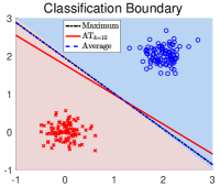
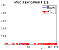
(a1)	(b1)	(c1)	(d1)
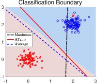
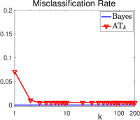
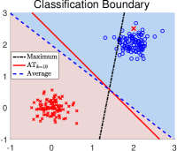
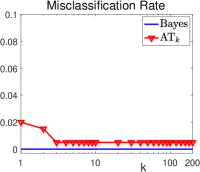
(a2)	(b2)	(c2)	(d2)
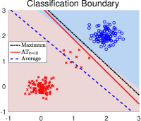
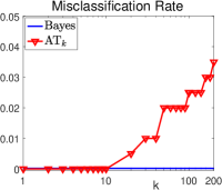
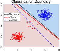
(a3)	(b3)	(c3)	(d3)
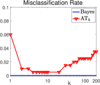
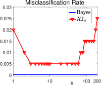
(a4)	(b4)	(c4)	(d4)
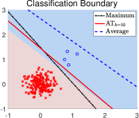
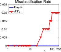
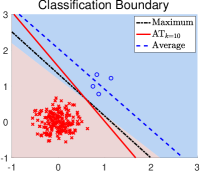
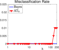
(a5)	(b5)	(c5)	(d5)
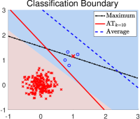
(a6)	(b6)	(c6)	(d6)

Figure 4: Comparison of different aggregate losses on 2D synthetic datasets for binary classification on six different data distributions. Each row refers to one data distribution. In all plots, the $+$ samples are red crosses and the $-$ samples are blue circles. The outliers are shown with an enlarged $\times$ if any. The plots on the left panel report the results of linear classifiers learned with different aggregate losses combined with individual logistic loss, and that on the right panel are the results of different aggregate losses combined with individual hinge loss. The plots on the first and third columns show the learned linear classifiers of maximum, average and AT_k=10 with the optimal Bayes classification shown as shaded areas, and the plots on the second and fourth columns show the misclassification rate of AT_k vs. $k$.

Sinc data used for regression: This dataset is drawn from sinc function, i.e., $y=\sin(x)/x$, where $x$ is an scalar, and the goal is to estimate $y$ from the input $x$. We randomly select $1000$ samples $(x_{i},y_{i})$ with $x_{i}$ drawn uniformly from $[-10,10]$. As we use linear regression model in our experiments, we map the input $x$ into a kernel space via the radial basis function (RBF) kernel. We select $10$ RBF kernels from $[-10,10]$, which leads to $10$-dimension input $\mathbf{x}=[k(x,c_{1}),\cdots,k(x,c_{10})]^{T}$, where $k(x,c_{i})=\exp(-(x-c_{i})^{2})$. We also add random Gaussian noise $N(0,0.2^{2})$ to the target output.

Table 3 tabulates the statistical information of datasets that used in this paper. Experiments results in terms of G-mean for binary classification are reported in Table 4, and experiments results in terms of mean absolute error (MAE) for regression are also reported in Table 5.

	Logistic Loss			Hinge Loss
	Maximum	Average	AT${}_{k^{\ast}}$	Maximum	Average	AT${}_{k^{\ast}}$
Monk	75.80(3.37)	79.47(2.05)	82.95(2.39)	76.37(3.51)	81.15(3.11)	82.68(2.79)
Australian	78.88(7.56)	86.10(3.19)	88.37(2.97)	78.99(7.47)	85.72(3.15)	87.50(4.14)
Madelon	51.20(2.92)	59.28(1.41)	60.26(1.58)	49.42(2.71)	59.36(1.83)	59.72(1.51)
Splice	76.31(1.94)	82.73(1.01)	83.90(0.97)	76.47(2.12)	83.78(1.12)	83.79(0.97)
Spambase	69.48(5.94)	90.63(1.21)	90.63(1.21)	69.96(6.76)	91.90(0.85)	91.90(0.85)
German	44.88(7.37)	60.12(7.59)	63.80(4.29)	44.87(7.34)	61.02(7.49)	62.96(3.33)
Titanic	46.52(15.27)	66.69(1.44)	66.69(1.44)	48.55(13.15)	66.65(1.43)	67.74(1.78)
Phoneme	19.10(11.84)	63.00(1.84)	66.29(2.04)	12.89(11.47)	70.41(1.65)	70.41(1.65)

Table 4: Average G-mean(%) of different learning objectives over $8$ datasets. The best results are shown in bold with results that are not significant different to the best results underlined.

	Square Loss			Absolute Loss
	Maximum	Average	AT${}_{k^{\ast}}$	Maximum	Average	AT${}_{k^{\ast}}$
Sinc	0.2438(0.0445)	0.0816(0.0045)	0.0806(0.0044)	0.1489(0.0466)	0.0827(0.0048)	0.0821(0.0055)
Housing	0.1198(0.0150)	0.0738(0.0075)	0.0736(0.0079)	0.1233(0.0127)	0.0713(0.0089)	0.0712(0.0088)
Abalone	0.1312(0.0919)	0.0575(0.0016)	0.0574(0.0015)	0.1082(0.0303)	0.0559(0.0014)	0.0557(0.0016)
Cpusmall	0.2404(0.0832)	0.0634(0.0027)	0.0627(0.0025)	0.1868(0.0997)	0.0423(0.0018)	0.0422(0.0018)

Table 5: Average MAE on four datasets. The best results are shown in bold with results that are not significant different to the best results underlined.

plain refs_apx

References

- [1] P. L. Bartlett, M. I. Jordan, and J. D. McAuliffe. Convexity, classification, and risk bounds. Journal of the American Statistical Association, 101(473):138–156, 2006.
- [2] Y. Bengio, J. Louradour, R. Collobert, and J. Weston. Curriculum learning. In ICML, pages 41–48, 2009.
- [3] O. Bousquet and L. Bottou. The tradeoffs of large scale learning. In NIPS, pages 161–168, 2008.
- [4] C.-C. Chang and C.-J. Lin. Libsvm: a library for support vector machines. TIST, 2(3):27, 2011.
- [5] C. Cortes and V. Vapnik. Support-vector networks. Machine learning, 20(3):273–297, 1995.
- [6] K. Crammer and Y. Singer. On the algorithmic implementation of multiclass kernel-based vector machines. Journal of machine learning research, 2(Dec):265–292, 2001.
- [7] E. De Vito, A. Caponnetto, and L. Rosasco. Model selection for regularized least-squares algorithm in learning theory. Foundations of Computational Mathematics, 5(1):59–85, 2005.
- [8] L. Devroye, L. Györfi, and G. Lugosi. A probabilistic theory of pattern recognition, volume 31. Springer Science & Business Media, 2013.
- [9] Y. Fan, R. He, J. Liang, and B.-G. Hu. Self-paced learning: An implicit regularization perspective. In AAAI, pages 1877–1833, 2017.
- [10] R. He, W.-S. Zheng, and B.-G. Hu. Maximum correntropy criterion for robust face recognition. IEEE Transactions on Pattern Analysis and Machine Intelligence, 33(8):1561–1576, 2011.
- [11] M. P. Kumar, B. Packer, and D. Koller. Self-paced learning for latent variable models. In NIPS, pages 1189–1197, 2010.
- [12] M. Lapin, M. Hein, and B. Schiele. Top-k multiclass SVM. In NIPS, pages 325–333, 2015.
- [13] M. Lapin, M. Hein, and B. Schiele. Loss functions for top-k error: Analysis and insights. In CVPR, pages 1468–1477, 2016.
- [14] Y. Lin. A note on margin-based loss functions in classification. Statistics & probability letters, 68(1):73–82, 2004.
- [15] H. Masnadi-Shirazi and N. Vasconcelos. On the design of loss functions for classification: theory, robustness to outliers, and savageboost. In NIPS, pages 1049–1056, 2009.
- [16] W. Ogryczak and A. Tamir. Minimizing the sum of the k largest functions in linear time. Information Processing Letters, 85(3):117–122, 2003.
- [17] C. Rudin. The p-norm push: A simple convex ranking algorithm that concentrates at the top of the list. Journal of Machine Learning Research, 10(Oct):2233–2271, 2009.
- [18] B. Schölkopf and A. J. Smola. Learning with kernels: support vector machines, regularization, optimization, and beyond. MIT press, 2001.
- [19] B. Schölkopf, A. J. Smola, R. C. Williamson, and P. L. Bartlett. New support vector algorithms. Neural computation, 12(5):1207–1245, 2000.
- [20] S. Shalev-Shwartz and Y. Wexler. Minimizing the maximal loss: How and why. In ICML, 2016.
- [21] N. Srebro and A. Tewari. Stochastic optimization for machine learning. ICML Tutorial, 2010.
- [22] I. Steinwart. On the optimal parameter choice for -support vector machines. IEEE Transactions on Pattern Analysis and Machine Intelligence, 25(10):1274–1284, 2003.
- [23] I. Steinwart and A. Christmann. Support vector machines. Springer Science & Business Media, 2008.
- [24] N. Usunier, D. Buffoni, and P. Gallinari. Ranking with ordered weighted pairwise classification. In ICML, pages 1057–1064, 2009.
- [25] V. Vapnik. Statistical learning theory, volume 1. Wiley New York, 1998.
- [26] Q. Wu, Y. Ying, and D.-X. Zhou. Learning rates of least-square regularized regression. Foundations of Computational Mathematics, 6(2):171–192, 2006.
- [27] Y. Wu and Y. Liu. Robust truncated hinge loss support vector machines. Journal of the American Statistical Association, 102(479):974–983, 2007.
- [28] Y. Yu, M. Yang, L. Xu, M. White, and D. Schuurmans. Relaxed clipping: A global training method for robust regression and classification. In NIPS, pages 2532–2540, 2010.