From source to target and back: Symmetric Bi-Directional Adaptive GAN

Abstract

The effectiveness of GANs in producing images according to a specific visual domain has shown potential in unsupervised domain adaptation. Source labeled images have been modified to mimic target samples for training classifiers in the target domain, and inverse mappings from the target to the source domain have also been evaluated, without new image generation.

In this paper we aim at getting the best of both worlds by introducing a symmetric mapping among domains. We jointly optimize bi-directional image transformations combining them with target self-labeling. We define a new class consistency loss that aligns the generators in the two directions, imposing to preserve the class identity of an image passing through both domain mappings. A detailed analysis of the reconstructed images, a thorough ablation study and extensive experiments on six different settings confirm the power of our approach.

1 Introduction

The ability to generalize across domains is challenging when there is ample labeled data on which to train a deep network (source domain), but no annotated data for the target domain. To attack this issue, a wide array of methods have been proposed, most of them aiming at reducing the shift between the source and target distributions (see Sec. 2 for a review of previous work). An alternative is mapping the source data into the target domain, either by modifying the image representation [10] or by directly generating a new version of the source images [4]. Several authors proposed approaches that follow both these strategies by building over Generative Adversarial Networks (GANs) [13]. A similar but inverse method maps the target data into the source domain, where there is already an abundance of labeled images [39].

We argue that these two mapping directions should not be alternative, but complementary. Indeed, the main ingredient for adaptation is the ability of transferring successfully the style of one domain to the images of the other. This, given a fixed generative architecture, will depend on the application: there may be cases where mapping from the source to the target is easier, and cases where it is true otherwise. By pursuing both directions in a unified architecture, we can obtain a system more robust and more general than previous adaptation algorithms.

With this idea in mind, we designed SBADA-GAN: Symmetric Bi-Directional ADAptive Generative Adversarial Network. Its distinctive features are (see Figure 1 for a schematic overview):

• it exploits two generative adversarial losses that encourage the network to produce target-like images from the source samples and source-like images from the target samples. Moreover, it jointly minimizes two classification losses, one on the original source images and the other on the transformed target-like source images;

• it uses the source classifier to annotate the source-like transformed target images. Such pseudo-labels help regularizing the same classifier while improving the target-to-source generator model by backpropagation;

• it introduces a new semantic constraint on the source images: the class consistency loss. It imposes that by mapping source images towards the target domain and then again towards the source domain they should get back to their ground truth class. This last condition is less restrictive than a standard reconstruction loss [41, 18], as it deals only with the image annotation and not with the image appearance. Still, our experiments show that it is highly effective in aligning the domain mappings in the two directions;

• at test time the two trained classifiers are used respectively on the original target images and on their source-like transformed version. The two predictions are integrated to produce the final annotation.

Our architecture yields realistic image reconstructions while competing against previous state-of-the-art classifiers and exceeding them on four out of six different unsupervised adaptation settings. An ablation study showcasing the importance of each component in the architecture, and investigating the robustness with respect to its hyperparameters, sheds light on the inner workings of the approach, while providing further evidence of its value.

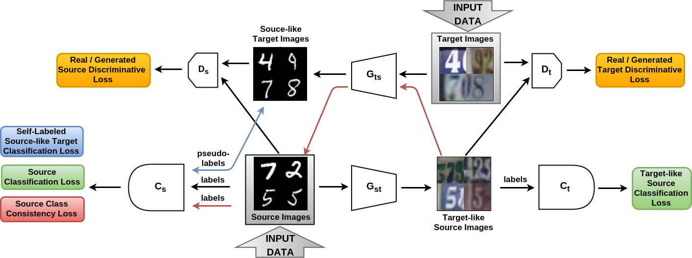
Figure 1: SBADA-GAN, training: the data flow starts from the source and target images indicated by the Input Data arrows. The bottom and top row show respectively the source-to-target and target-to-source symmetric directions. The generative models $G_{st}$ and $G_{ts}$ transform the source images to the target domain and vice versa. $D_{s}$ and $D_{t}$ discriminate real from generated images of source and target. Finally the classifiers $C_{s}$ and $C_{t}$ are trained to recognize respectively the original source images and their target-like transformed versions. The bi-directional blue arrow indicates that the source-like target images are automatically annotated and the assigned pseudo-labels are re-used by the classifier $C_{s}$. The red arrows describe the class consistency condition by which source images transformed to the target domain through $G_{st}$ and back to the source domain through $G_{ts}$ should maintain their ground truth label.

2 Related Work

GANs

Generative Adversarial Networks are composed of two modules, a generator and a discriminator. The generator’s objective is to synthesize samples whose distribution closely matches that of real data, while the discriminator objective is to distinguish real from generated samples. GANs are agnostic to the training samples labels, while conditional GAN variants [25] exploit the class annotation as additional information to both the generator and the discriminator. Some works used multiple GANs: in CoGAN [22] two generators and two discriminators are coupled by weight-sharing to learn the joint distribution of images in two different domains without using pair-wise data. Cycle-GAN [41], Disco-GAN [18] and UNIT [21] encourage the mapping between two domains to be well covered by imposing transitivity: the mapping in one direction followed by the mapping in the opposite direction should arrive where it started. For this image generation process the main performance measure is either a human-based quality control or scores that evaluate the interpretability of the produced images by pre-existing models [31, 41].

Domain Adaptation

A widely used strategy consists in minimizing the difference between the source and target distributions [38, 36, 7]. Alternative approaches minimize the errors in target samples reconstruction [12] or impose a consistency condition so that neighboring target samples assigned to different labels are penalized proportionally to their similarity [33]. Very recently, [15] proposed to enforce associations between source and target samples of the same ground truth or predicted class, while [30] assigned pseudo-labels to target samples using an asymmetric tri-training method.

Domain invariance can be also treated as a binary classification problem through an adversarial loss inspired by GANs, which encourages mistakes in domain prediction [10]. For all the methods adopting this strategy, the described losses are minimized jointly with the main classification objective function on the source task, guiding the feature learning process towards a domain invariant representation. Only in [39] the two objectives are kept separated and recombined in a second step. In [5] the feature components that differentiate two domains are modeled separately from those shared among them.

Image Generation for Domain Adaptation

In the first style transfer methods [11, 17] new images were synthesized to maintain a specific content while replicating the style of one or a set of reference images. Similar transfer approaches have been used to generate images with different visual domains. In [34] realistic samples were generated from synthetic images and the produced data could work as training set for a classification model with good results on real images. [4] proposed a GAN-based approach that adapts source images to appear as if drawn from the target domain; the classifier trained on such data outperformed several domain adaptation methods by large margins. [37] introduced a method to generate source images that resemble the target ones, with the extra consistency constraint that the same transformation should keep the target samples identical. All these methods focus on the source-to-target image generation, not considering adding an inverse procedure, from target to source, which we show instead to be beneficial.

3 Method

Model

We focus on unsupervised cross domain classification. Let us start from a dataset $\bm{X}_{s}=\{\bm{x}^{i}_{s},y^{i}_{s}\}_{i=0}^{N_{s}}$ drawn from a labeled source domain $\mathcal{S}$, and a dataset $\bm{X}_{t}=\{\bm{x}^{j}_{t}\}_{j=0}^{N_{t}}$ from a different unlabeled target domain $\mathcal{T}$, sharing the same set of categories. The task is to maximize the classification accuracy on $\bm{X}_{t}$ while training on $\bm{X}_{s}$. To reduce the domain gap, we propose to adapt the source images such that they appear as sampled from the target domain by training a generator model $G_{st}$ that maps any source samples $\bm{x}^{i}_{s}$ to its target-like version $\bm{x}^{i}_{st}=G_{st}(\bm{x}^{i}_{s})$ defining the set $\bm{X}_{st}=\{\bm{x}^{i}_{st},y^{i}_{s}\}_{i=0}^{N_{s}}$ (see Figure 1, bottom row). The model is also augmented with a discriminator $D_{t}$ and a classifier $C_{t}$. The former takes as input the target images $\bm{X}_{t}$ and target-like source transformed images $\bm{X}_{st}$, learning to recognize them as two different sets. The latter takes as input each of the transformed images $\bm{x}^{i}_{st}$ and learns to assign its task-specific label $y^{i}_{s}$. During the training procedure for this model, information about the domain recognition likelihood produced by $D_{t}$ is used adversarially to guide and optimize the performance of the generator $G_{st}$. Similarly, the generator also benefits from backpropagation in the classifier training procedure.

Besides the source-to-target transformation, we also consider the inverse target-to-source direction by using a symmetric architecture (see Figure 1, top row). Here any target image $\bm{x}^{j}_{t}$ is given as input to a generator model $G_{ts}$ transforming it to its source-like version $\bm{x}^{j}_{ts}=G_{ts}(\bm{x}^{j}_{t})$, defining the set $\bm{X}_{ts}=\{\bm{x}^{j}_{ts}\}_{j=0}^{N_{t}}$. As before, the model is augmented with a discriminator $D_{s}$ which takes as input both $\bm{X}_{ts}$ and $\bm{X}_{s}$ and learns to recognize them as two different sets, adversarially helping the generator.

Since the target images are unlabeled, no classifier can be trained in the target-to-source direction as a further support for the generator model. We overcome this issue by self-labeling (see Figure 1, blue arrow). The original source data $\bm{X}_{s}$ is used to train a classifier $C_{s}$. Once it has reached convergence, we apply the learned model to annotate each of the source-like transformed target images $\bm{x}^{j}_{ts}$. These samples, with the assigned pseudo-labels $y^{j}_{t_{self}}=\operatornamewithlimits{argmax}_{y}(C_{s}(G_{ts}(\bm{x}^{j}_{t}))$, are then used transductively as input to $C_{s}$ while information about the performance of the model on them is backpropagated to guide and improve the generator $G_{ts}$. Self-labeling has a long track record of success for domain adaptation: it proved to be effective both with shallow models [6, 14, 27], as well as with the most recent deep architectures [33, 38, 30]. In our case the classification loss on pseudo-labeled samples is combined with our other losses, which helps making sure we move towards the optimal solution: in case of a moderate domain shift, the correct pseudo-labels help to regularize the learning process, while in case of large domain shift, the possible mislabeled samples do not hinder the performance (see Sec. 4.5 for a detailed discussion on the experimental results).

Finally, the symmetry in the source-to-target and target-to-source transformations is enhanced by aligning the two generator models such that, when used in sequence, they bring a sample back to its starting point. Since our main focus is classification, we are interested in preserving the class identity of each sample rather than its overall appearance. Thus, instead of a standard image-based reconstruction condition we introduce a class consistency condition (see Figure 1, red arrows). Specifically, we impose that any source image $\bm{x}^{i}_{s}$ adapted to the target domain through $G_{st}(\bm{x}^{i}_{s})$ and transformed back towards the source domain through $G_{ts}(G_{st}(\bm{x}^{i}_{s}))$ is correctly classified by $C_{s}$. This condition helps by imposing a further joint optimization of the two generators.

Learning

Here we formalize the description above. To begin with, we specify that the generators take as input a noise vector $\bm{z}\in\mathcal{N}(0,1)$ besides the images, this allows some extra degree of freedom to model external variations. We also better define the discriminators as $D_{s}(\bm{x})$, $D_{t}(\bm{x})$ and the classifiers as $C_{s}(\bm{x})$, $C_{t}(\bm{x})$. Of course each of these models depends from its parameters but we do not explicitly indicate them to simplify the notation. For the same reason we also drop the superscripts $i,j$.

The source-to-target part of the network optimizes the following objective function:

$$\min_{{G_{st}},{C_{t}}}\max_{{D_{t}}}~{}~{}\alpha\mathcal{L}_{D_{t}}(D_{t},G_{st})+\beta\mathcal{L}_{C_{t}}(G_{st},C_{t})~{},$$ (1)

where the classification loss $\mathcal{L}_{C_{t}}$ is a standard softmax cross-entropy

$$\mathcal{L}_{C_{t}}(G_{st},C_{t})=\mathbb{E}_{\begin{subarray}{c}\{\bm{x}_{s},\bm{y}_{s}\}\sim\mathcal{S}\\ \bm{z}_{s}\sim noise\end{subarray}}[{-\bm{y}_{s}}\cdot\log({\hat{\bm{y}}_{s}})]~{},$$ (2)

evaluated on the source samples transformed by the generator $G_{st}$, so that $\hat{\bm{y}}_{s}=C_{t}(G_{st}(\bm{x}_{s},\bm{z}_{s}))$ and $\bm{y}_{s}$ is the one-hot encoding of the class label $y_{s}$. For the discriminator, instead of the less robust binary cross-entropy, we followed [24] and chose a least square loss:

$$\mathcal{L}_{D_{t}}(D_{t},G_{st})= \mathbb{E}_{\bm{x}_{t}\sim T}[(D_{t}(\bm{x}_{t})-1)^{2}]+$$

$$\mathbb{E}_{\begin{subarray}{c}\bm{x}_{s}\sim S\\ \bm{z}_{s}\sim noise\end{subarray}}[(D_{t}(G_{st}(\bm{x}_{s},\bm{z}_{s})))^{2}]~{}.$$ (3)

The objective function for the target-to-source part of the network is:

$$\min_{{G_{ts}},{C_{s}}}\max_{{D_{s}}}~{}~{} \gamma\mathcal{L}_{D_{s}}(D_{s},G_{ts})+$$

$$\mu\mathcal{L}_{C_{s}}(C_{s})+\eta\mathcal{L}_{self}(G_{ts},C_{s})~{},$$ (4)

where the discriminative loss is analogous to eq. (3), while the classification loss is analogous to eq. (2) but evaluated on the original source samples with $\hat{\bm{y}}_{s}=C_{s}(\bm{x}_{s})$, thus it neither has any dependence on the generator that transforms the target samples $G_{ts}$, nor it provides feedback to it. The self loss is again a classification softmax cross-entropy:

$$\mathcal{L}_{self}(G_{ts},C_{s})=\mathbb{E}_{\begin{subarray}{c}\{\bm{x}_{t},\bm{y}_{t_{self}}\}\sim\mathcal{T}\\ \bm{z}_{t}\sim noise\end{subarray}}[-\bm{y}_{t_{self}}\cdot\log({\hat{\bm{y}}_{t_{self}}})]~{}.$$ (5)

where $\hat{\bm{y}}_{t_{self}}=C_{s}(G_{ts}(\bm{x}_{t},\bm{z}_{t}))$ and $\bm{y_{t_{self}}}$ is the one-hot vector encoding of the assigned label ${y_{t_{self}}}$. This loss back-propagates to the generator $G_{ts}$ which is encouraged to preserve the annotated category within the transformation.

Finally, we developed a novel class consistency loss by minimizing the error of the classifier $C_{s}$ when applied on the concatenated transformation of $G_{ts}$ and $G_{st}$ to produce $\hat{\bm{y}}_{cons}=(C_{s}(G_{ts}(G_{st}(\bm{x}_{s},\bm{z}_{s}),\bm{z}_{t})))$:

$$\mathcal{L}_{cons}(G_{ts},G_{st},C_{s})=\mathbb{E}_{\begin{subarray}{c}\{\bm{x}_{s},\bm{y}_{s}\}\sim S\\ \bm{z}_{s},\bm{z}_{t}\sim noise\end{subarray}}[{-\bm{y}_{s}}\cdot\log({\hat{\bm{y}}_{cons}})]~{}.$$ (6)

This loss has the important role of aligning the generators in the two directions and strongly connecting the two main parts of our architecture.

By collecting all the presented parts, we conclude with the complete SBADA-GAN loss:

$$\mathcal{L}_{SBADA-GAN}(G_{st},G_{ts},C_{s},C_{t},D_{s},D_{t})=~{}~{}~{}~{}~{}~{}~{}~{}~{}~{}~{}~{}~{}~{}$$

$$\alpha\mathcal{L}_{D_{t}}+\beta\mathcal{L}_{C_{t}}+\gamma\mathcal{L}_{D_{s}}+\mu\mathcal{L}_{C_{s}}+\eta\mathcal{L}_{self}+\nu\mathcal{L}_{cons}~{}.$$ (7)

Here $(\alpha,\beta,\gamma,\mu,\eta,\nu)\geq 0$ are weights that control the interaction of the loss terms. While the combination of six different losses might appear daunting, it is not unusual [5]. Here, it stems from the symmetric bi-directional nature of the overall architecture. Indeed each directional branch has three losses as it is custom practice in the GAN-based domain adaptation literature [39, 4]. Moreover, the ablation study reported in Sec. 4.5 indicates that the system is remarkably robust to changes in the hyperparameter values.

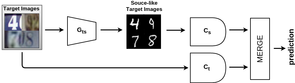
Figure 2: SBADA-GAN, test: the two pre-trained classifiers are applied respectively on the target images and on the transformed source-like target images. Their outputs are linearly combined for the final prediction.

Testing

The classifier $C_{t}$ is trained on $\bm{X}_{st}$ generated images that mimic the target domain style, and is then tested on the original target samples $\bm{X}_{t}$. The classifier $C_{s}$ is trained on $\bm{X}_{s}$ source data, and then tested on $\bm{X}_{ts}$ samples, that are the target images modified to mimic the source domain style. These classifiers make mistakes of different type assigning also a different confidence rank to each of the possible labels. Overall the two classification models complement each other. We take advantage of this with a simple ensemble method $~{}\sigma C_{s}(G_{ts}(\bm{x}_{t},\bm{z}_{t}))+\tau C_{t}(\bm{x}_{t})~{}$ which linearly combines their probability output, providing a further gain in performance. A schematic illustration of the testing procedure is shown in Figure 2. We set the combination weights $\sigma,\tau$ through cross validation (see Sec. 4.2 for further details).

4 Evaluation

4.1 Datasets and Adaptation Scenarios

We evaluate SBADA-GAN on several unsupervised adaptation scenarios, considering the following widely used digits datasets and settings:

MNIST $\rightarrow$ MNIST-M:

MNIST [20] contains centered, $28\times 28$ pixel, grayscale images of single digit numbers on a black background, while MNIST-M [10] is a variant where the background is substituted by a randomly extracted patch obtained from color photos of BSDS500 [3]. We follow the evaluation protocol of [5, 4, 10].

MNIST $\leftrightarrow$ USPS:

USPS [9] is a digit dataset automatically scanned from envelopes by the U.S. Postal Service containing a total of 9,298 $16\times 16$ pixel grayscale samples. The images are centered, normalized and show a broad range of font styles. We follow the evaluation protocol of [4].

SVHN $\leftrightarrow$ MNIST:

SVHN [28] is the challenging real-world Street View House Number dataset, much larger in scale than the other considered datasets. It contains over $600k$ $32\times 32$ pixel color samples. Besides presenting a great variety of styles (in shape and texture), images from this dataset often contain extraneous numbers in addition to the labeled, centered one. Most previous works simplified the data by considering a grayscale version, instead we apply our method to the original RGB images. Specifically for this experiment we resize the MNIST images to $32\times 32$ pixels and use the protocol by [5, 12].

We also test SBADA-GAN on a traffic sign scenario.
Synth Signs $\rightarrow$ GTSRB: the Synthetic Signs collection [26] contains $100k$ samples of common street signs obtained from Wikipedia and artificially transformed to simulate various imaging conditions. The German Traffic Signs Recognition Benchmark (GTSRB, [35]) consists of $51,839$ cropped images of German traffic signs. Both databases contain samples from $43$ classes, thus defining a larger classification task than that on the $10$ digits. For the experiment we adopt the protocol proposed in [15].

	MNIST$\rightarrow$ USPS	USPS$\rightarrow$MNIST	MNIST$\rightarrow$MNIST-M	SVHN$\rightarrow$MNIST	MNIST$\rightarrow$SVHN	Synth Signs$\rightarrow$GTSRB
Source Only	78.9	57.1 $\pm$ 1.7	63.6	60.1 $\pm$ 1.1	26.0 $\pm$ 1.2	79.0
CORAL [36]	81.7	-	57.7	63.1	-	86.9
MMD [38]	81.1	-	76.9	71.1	-	91.1
DANN [10]	85.1	73.0 $\pm$ 2.0	77.4	73.9	35.7	88.7
DSN [5]	91.3	-	83.2	82.7	-	93.1
CoGAN [22]	91.2	89.1 $\pm$ 0.8	62.0	not conv.	-	-
ADDA [39]	89.4 $\pm$ 0.2	90.1 $\pm$ 0.8	-	76.0 $\pm$ 1.8	-	-
DRCN [12]	91.8 $\pm$ 0.1	73.7 $\pm$ 0.1	-	82.0 $\pm$ 0.2	40.1 $\pm$ 0.1	-
PixelDA [4]	95.9	-	98.2	-	-	-
DTN [37]	-	-	-	84.4	-	-
TRUDA [33]	-	-	86.7	78.8	40.3	-
ATT [30]	-	-	94.2	86.2	52.8	96.2
UNIT [21]	95.9	93.5	-	90.5	-	-
DAass fix. par. [15]	-	-	89.5	95.7	-	82.8
DAass [15]	-	-	89.5	97.6	-	97.7
Target Only	96.5	99.2 $\pm$ 0.1	96.4	99.5	96.7	98.2
SBADA-GAN $C_{t}$	96.7	94.4	99.1	72.2	59.2	95.9
SBADA-GAN $C_{s}$	97.1	87.5	98.4	74.2	50.9	95.7
SBADA-GAN	97.6	95.0	99.4	76.1	61.1	96.7
GenToAdapt [32]	92.5 $\pm$ 0.7	90.8 $\pm$ 1.3	-	84.7 $\pm$ 0.9	36.4 $\pm$ 1.2	-
CyCADA [1]	94.8 $\pm$ 0.2	95.7 $\pm$ 0.2	-	88.3 $\pm$ 0.2	-	-
Self-Ensembling [2]	98.3 $\pm$ 0.1	99.5 $\pm$ 0.4	-	99.2 $\pm$ 0.3	42.0 $\pm$ 5.7	98.3 $\pm$ 0.3

Table 1: Comparison against previous work. SBADA-GAN $C_{t}$ reports the accuracies produced by the classifier trained in the target domain space. Similarly, SBADA-GAN $C_{s}$ reports the results produced by the classifier trained in the source domain space and tested on the target images mapped to this space. SBADA-GAN reports the results obtained by a weighted combination of the softmax outputs of these two classifiers. Note that all competitors convert SVHN to grayscale, while we deal with the more complex original RGB version. The last three rows report results from online available pre-print papers.

4.2 Implementation details

We composed SBADA-GAN starting from two symmetric GANs, each with an architecture analogous to that used for the PixelDA model [4].

The model is coded in python and we ran all our experiments in the Keras framework [8] (code will be made available upon acceptance). We use the ADAM [19] optimizer with learning rates for the discriminator and the generator both set to $10^{-4}$. The batch size is set to $32$ and we train the model for $500$ epochs not noticing any overfitting, which suggests that further epochs might be beneficial. The $\alpha$ and $\gamma$ loss weights (discriminator losses) are set to $1$, $\beta$ and $\mu$ (classifier losses) are set to $10$, to prevent that generator from indirectly switching labels (for instance, transform $7$’s into $1$’s). The class consistency loss weight $\nu$ is set to $1$. All training procedures start with the self-labeling loss weight, $\eta$, set to zero, as this loss hinders convergence until the classifier is fully trained. After the model converges (losses stop oscillating, usually after $250$ epochs) $\eta$ is set to $1$ to further increase performance. Finally the parameters to combine the classifiers at test time are $\sigma\in[0,0.1,0.2,\ldots,1]$ and $\tau=(1-\sigma)$ chosen on a validation set of 1000 random samples from the target in each different setting.

4.3 Quantitative Results

Table 1 shows results on our six evaluation settings. The top of the table reports results by thirteen competing baselines published over the last two years. The Source-Only and Target-Only rows contain reference results corresponding to the naïve no-adaptation case and to the target fully supervised case. For SBADA-GAN, besides the full method, we also report the accuracy obtained by the separate classifiers (indicated by $C_{s}$ and $C_{t}$) before the linear combination. The last three rows show results that appeared recently in pre-prints available online.

SBADA-GAN improves over the state of the art in four out of six settings. In these cases the advantage with respect to its competitors is already visible in the separate $C_{s}$ and $C_{t}$ results and it increases when considering the full combination procedure. Moreover, the gain in performance of SBADA-GAN reaches up to $+8$ percentage points in the MNIST$\rightarrow$SVHN experiment. This setting was disregarded in many previous works: differently from its inverse SVHN$\rightarrow$MNIST, it requires a difficult adaptation from the grayscale handwritten digits domain to the widely variable and colorful street view house number domain. Thanks to its bi-directionality, SBADA-GAN leverages on the inverse target to source mapping to produce highly accuracy results.

Conversely, in the SVHN$\rightarrow$MNIST case SBADA-GAN ranks eighth out of the thirteen baselines in terms of performance. Our accuracy is on par with ADDA’s [39]: the two approaches share the same classifier architecture, although the number of fully-connected neurons of SBADA-GAN is five time lower. Moreover, compared to DRCN [12], the classifiers of SBADA-GAN are shallower with a reduced number of convolutional layers. Overall here SBADA-GAN suffers of some typical drawbacks of GAN-based domain adaptation methods: although the style of a domain can be easily transferred in the raw pixel space, the generative process does not have any explicit constraint on reducing the overall data distribution shift as instead done by the alternative feature-based domain adaptation approaches. Thus, methods like DA_ass [15], DTN [37] and DSN [5] deal better with the large domain gap of the SVHN$\rightarrow$MNIST setting.

Finally, in the Synth Signs $\rightarrow$ GTSRB experiment, SBADA-GAN is just slightly worse than DA_ass, but outperforms all the other competing methods. The comparison remains in favor of SBADA-GAN when considering that its performance is robust to hyperparameter variations (see Sec. 4.5 for more details), while the performance of DA_ass drops significantly in case of not tuned, pre-defined fixed parameters.

4.4 Qualitative Results

To complement the quantitative evaluation, we look at the quality of the images generated by SBADA-GAN. First, we see from Figure 3 how the generated images actually mimic the style of the chosen domain, even when going from the simple MNIST digits to the SVHN colorful house numbers.

Visually inspecting the data distribution before and after domain mapping defines a second qualitative evaluation metric. We use t-SNE [23] to project the data from their raw pixel space to a simplified 2D embedding. Figure 6 shows such visualizations and indicates that the transformed dataset tends to replicate faithfully the distribution of the chosen final domain.

A further measure of the quality of the SBADA-GAN generators comes from the diversity of the produced images. Indeed, a well-known failure mode of GANs is that the generator may collapse and output a single prototype that maximally fools the discriminator. To evaluate the diversity of samples generated by SBADA-GAN we choose the Structural Similarity (SSIM, [40]), a measure that correlates well with the human perceptual similarity judgments. Its values range between $0$ and $1$ with higher values corresponding to more similar images. We follow the same procedure used in [29] by randomly choosing $1000$ pairs of generated images within a given class. We also repeat the evaluation over all the classes and calculate the average results. Table 2 shows the results of the mean SSIM metric and indicates that the SBADA-GAN generated images not only mimic the same style, but also successfully reproduce the variability of a chosen domain.

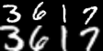
(a) MNIST to USPS

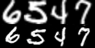
(b) USPS to MNIST

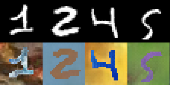
(c) MNIST to MNIST-M

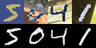
(d) MNIST-M to MNIST

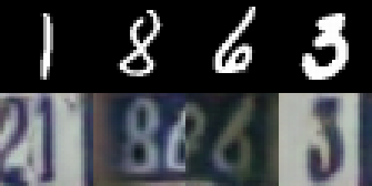
(e) MNIST to SVHN

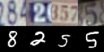
(f) SVHN to MNIST

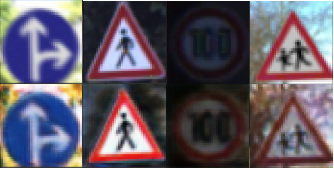
(g) Synth S. to GTSRB

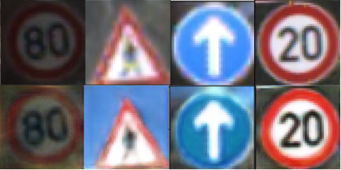
(h) GTSRB to Synth S.

Figure 3: Examples of generated digits: we show the image transformation from the original domain to the paired one as indicated under every sub-figure. For each of the (a)-(h) cases, the original/generated images are in the top/bottom row.

Setting	S	T map to S	S map to T	T
MNIST $\rightarrow$ USPS	$0.206$	$0.219$	$0.106$	$0.102$
MNIST $\rightarrow$ MNIST-M	$0.206$	$0.207$	$0.035$	$0.032$
MNIST $\rightarrow$ SVHN	$0.206$	$0.292$	$0.027$	$0.012$
Synth S. $\rightarrow$ GTSRB	$0.105$	$0.136$	$0.128$	$0.154$

Table 2: Dataset mean SSIM: this measure of data variability suggests that our method successfully generates images with not only the same style of a chosen domain, but also similar perceptual variability.

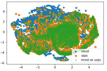
(a) MNIST to USPS

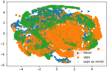
(b) USPS to MNIST

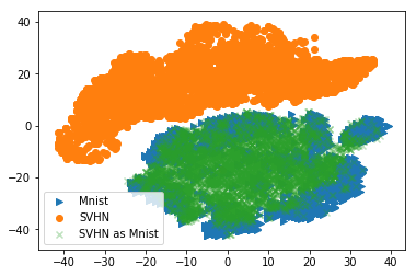
(c) SVHN to MNIST

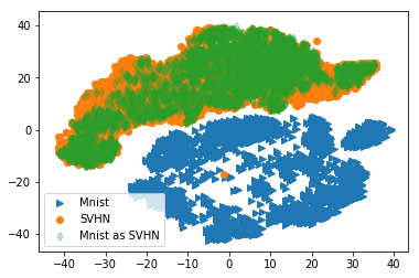
(d) MNIST to SVHN

Figure 4: t-SNE visualization of source, target and source mapped to target images. Note how the mapped source covers faithfully the target space both in the (a),(b) case with moderated domain shift and in the more challenging (c),(d) setting.

4.5 Ablation and Robustness Study

To clarify the role of each component in SBADA-GAN we go back to its core source-to-target single GAN module and analyze the effect of adding all the other model parts. Specifically we start by adding the symmetric target-to-source GAN model. These two parts are then combined and the domain transformation loop is closed by adding the class consistency condition. Finally the model is completed by introducing the target self-labeling procedure. We empirically test each of these model reconstruction steps on the MNIST$\rightarrow$USPS setting and report the results in Table 4.5. We see the gain achieved by progressively adding the different model components, with the largest advantage obtained by the introduction of self-labeling.

An analogous boost due to self-labeling is also visible in all the other experimental settings with the exception of MNIST$\leftrightarrow$SVHN, where the accuracy remains unchanged if $\eta$ is equal or larger than zero. A further analysis reveals that here the recognition accuracy of the source classifier applied to the source-like transformed target images is quite low (about $65\%$, while in all the other settings reaches $80-90\%$), thus the pseudo-labels cannot be considered reliable. Still, using them does not hinder the overall performance.

S$\rightarrow$T							T$\rightarrow$S	Class	Self	Accuracy
GAN							GAN	Consist.	Label.
$\mathcal{L}_{D_{t}}$	$\mathcal{L}_{C_{t}}$	$\mathcal{L}_{D_{s}}$	$\mathcal{L}_{C_{s}}$	$\mathcal{L}_{cons}$	$\mathcal{L}_{self}$	MNIST$\rightarrow$USPS
$\checkmark$	$\checkmark$					94.23
		$\checkmark$	$\checkmark$			91.55
$\checkmark$	$\checkmark$	$\checkmark$	$\checkmark$			94.90
$\checkmark$	$\checkmark$	$\checkmark$	$\checkmark$	$\checkmark$		95.45
$\checkmark$	$\checkmark$	$\checkmark$	$\checkmark$	$\checkmark$	$\checkmark$	97.60

Table 3: Analysis of the role of each SBADA-GAN component. We ran experiments by turning on the different losses of the model as indicated by the checkmarks.

The crucial effect of the class consistency loss can be better observed by looking at the generated images and comparing them with those obtained in two alternative cases: setting $\nu=0$, i.e. not using any consistency condition between the two generators $G_{st}$ and $G_{ts}$, or substituting our class consistency loss with the standard cycle consistency loss [41, 18] based on image reconstruction. For this evaluation we choose the MNIST$\rightarrow$SVHN case which has the strongest domain shift and we show the generated images in Figure 5. When the consistency loss is not activated, the $G_{ts}$ output images are realistic, but fail at reproducing the correct input digit and provide misleading information to the classifier. On the other hand, using the cycle-consistency loss preserves the input digit but fails in rendering a realistic sample in the correct domain style. Finally, our class consistency loss allows to preserve the distinct features belonging to a category while still leaving enough freedom to the generation process, thus it succeeds in both preserving the digits and rendering realistic samples.

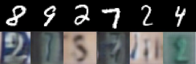
(a)

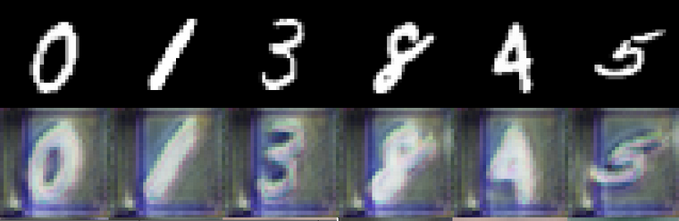
(b)

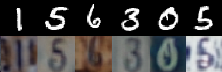
(c)

(d)

Figure 5: $G_{ts}$ outputs (lower line) and their respective inputs (upper line) obtained with: (a) no consistency loss, (b) image-based cycle consistency loss [41, 18], (c) our class consistency loss. In (d) we show some real SVHN samples as a reference.

About the class consistency loss, we also note that SBADA-GAN is robust to the specific choice of the weight $\nu$, given that it is different from zero. Changing it in $[0.1,1,10]$ induces a maximum variation of $0.6$ percentage points in accuracy over the different settings. An analogous evaluation performed on the classification loss weights $\beta$ and $\mu$ reveals that changing them in the same range used for $\nu$ causes a maximum overall performance variation of $0.2$ percentage points. Furthermore SBADA-GAN is minimally sensitive to the batch size used: halving it from $32$ to $16$ samples while keeping the same number of learning epochs reduces the performance only of about $0.2$ percentage points. Such robustness is particularly relevant when compared to competing methods. For instance the most recent $DA_{ass}$ [15] needs a perfectly balanced source and target distribution of classes in each batch, a condition difficult to satisfy in real world scenarios, and halving the originally large batch size reduces by $3.5$ percentage points the final accuracy. Moreover, changing the weights of the losses that enforce associations across domains with a range analogous to that used for the SBADA-GAN parameters induces a drop in performance up to $16$ accuracy percentage points.

5 Conclusion

This paper presented SBADA-GAN, an adaptive adversarial domain adaptation architecture that maps simultaneously source samples into the target domain and vice versa with the aim to learn and use both classifiers at test time. To achieve this, we proposed to use self-labeling to regularize the classifier trained on the source, and we impose a class consistency loss that improves greatly the stability of the architecture, as well as the quality of the reconstructed images in both domains.

We explain the success of SBADA-GAN in several ways. To begin with, thanks to the the bi-directional mapping we avoid deciding a priori which is the best strategy for a specific task. Also, the combination of the two network directions improves performance providing empirical evidence that they are learning different, complementary features. Our class consistency loss aligns the image generators, allowing both domain transfers to influence each other. Finally the self-labeling procedure boost the performance in case of moderate domain shift without hindering it in case of large domain gaps.

Acknowledgments

This work was supported by the ERC grant 637076 - RoboExNovo.

Appendix

Appendix A SBADA-GAN network architecture

We composed SBADA-GAN starting from two symmetric GANs, each with an architecture analogous to that used for the PixelDA model. Specifically

• the generators take the form of a convolutional residual network with four residual blocks each composed by two convolutional layers with 64 features;

• the input noise $\bm{z}$ is a vector of $N^{z}$ elements each sampled from a normal distribution $z_{i}\sim\mathcal{N}(0,1)$. It is fed to a fully connected layer which transforms it to a channel of the same resolution as that of the image, and is subsequently concatenated to the input as an extra channel. In all our experiments we used $N^{z}=5$;

• the discriminators are made of two convolutional layers, followed by an average pooling and a convolution that brings the discriminator output to a single scalar value;

• in both generator and discriminator networks, each convolution (with the exception of the last one of the generator) is followed by a batch norm layer [16];

• the classifiers have exactly the same structure of that in [4, 10];

• as activation functions we used ReLU in the generator and classifier, while we used leaky ReLU (with a $0.2$ slope) in the discriminator.

• all the input images to the generators are zero-centered and rescaled to $[-0.5,0.5]$. The images produced by the generators as well as the other input images to the classifiers and and the discriminators are zero-centered and rescaled to $[-127.5,127.5]$.

Thanks to the stability of the SBADA-GAN training protocol, we did not use any injected noise into the discriminators and we did not use any dropout layer.

Appendix B Experimental Settings

MNIST $\rightarrow$ MNIST-M:

MNIST has $60k$ images for training. As [4] we divided it into $50k$ samples for actual training and $10k$ for validation. All the $60k$ images from the MNIST-M training set were considered as test set. A subset of $1k$ images and their labels were also used to validate the classifier combination weights at test time.

USPS $\rightarrow$ MNIST:

USPS has $6,562$ training, $729$ validation, and $2,007$ test images. All of them were resized to $28\times 28$ pixels. The $60k$ training images of MNIST were considered as test set, with $1k$ samples and their labels also used for validation purposes.

MNIST $\rightarrow$ USPS:

even in this case MNIST training images were divided into $50k$ samples for actual training and $10k$ for validation. We tested on the whole set of $9,298$ images of USPS. Out of them, $1k$ USPS images and their labels were also used for validation.

SVHN $\rightarrow$ MNIST:

SVHN contains over $600k$ color images of which $73,257$ samples are used for training and $26,032$ for validation while the remaining data are somewhat less difficult samples. We disregarded this last set and considered only the first two. The $60k$ MNIST training samples were considered as test set, with $1k$ MNIST images and their labels also used for validation.

MNIST $\rightarrow$ SVHN:

for MNIST we used again the $50k$/$10k$ training/validation sets. The whole set of $99,289$ SVHN samples was considered for testing with $1k$ images and their labels also used for validation.

Synth Signs $\rightarrow$ GTSRB:

the Synth Signs dataset contains $100k$ images, out of which $90k$ were used for training and $10k$ for validation. The model was tested on the whole GTSRB dataset containing $51,839$ samples resized with bilinear interpolation to match the Synth Signs images’ size of $40\times 40$ pixels. Similarly to the previous cases, $1k$ GTSRB images and their labels were considered for validation purposes.

Appendix C Distribution Visualizations

To visualize the original data distributions and their respective transformations we used t-SNE [23]. The images were pre-processed by scaling in $[-1,1]$ and we applied PCA for dimensionality reduction from vectors with Width$\times$Height elements to $64$ elements. Finally t-SNE with default parameters was applied to project data to a 2-dimensional space.

The behavior shown by the t-SNE data visualization presented in the main paper extends also for the other experimental settings. We integrate here the visualization for the MNIST$\rightarrow$MNIST-M case in Figure 6. The plots show again a successful mapping with the generated data that cover faithfully the target space.

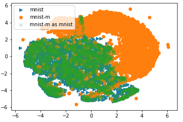
(a) MNIST-M to MNIST

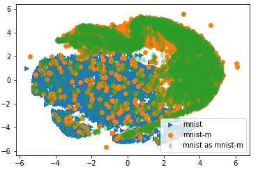
(b) MNIST to MNIST-M

Figure 6: t-SNE visualization of source, target and source mapped to target images. Note how the mapped source covers faithfully the target space in all the settings.

Appendix D Robustness experiments

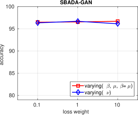
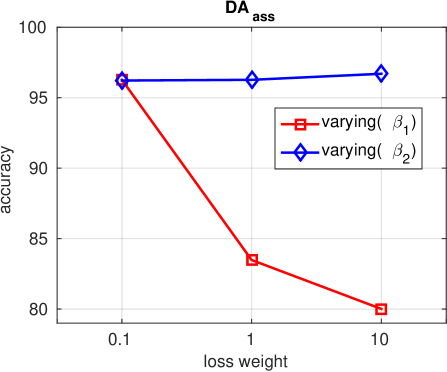
Figure 7: Behaviour of the SBADA-GAN and DA_ass methods when changing their loss weights. (left) for SBADA-GAN we kept $\alpha=\gamma=1$ and $\eta=1$, while we varied alternatively the weights of the classification losses $\beta,\mu$ with $\beta=\mu$ and keeping $\nu=1$, or the weight of the class consistency loss $\nu$ while fixing $\beta=\mu=10$. (right) for the DA_ass method we changed the weight of the walker loss $\beta_{1}$ while keeping that of the visit loss $\beta_{2}=0.1$, or alternatively we changed the weight of the visit loss $\beta_{2}$ while fixing that of the walker loss $\beta_{1}=1$.

The experiments about SBADA-GAN robustness to hyperparameters values are described at high level in Section 4.5 of the main paper submission. Here we report on the detailed results obtained on Synth. Signs $\rightarrow$ GTSRB when using SBADA-GAN and the DA_ass method [15].

For SBADA-GAN we keep fixed the weights of the discriminative losses $\alpha=\gamma=1$ as well as that of self-labeling $\eta=1$, while we varied alternatively the weights of the classification losses $\beta,\mu$ or the weight of the class consistency loss $\nu$ in $[0.1,1,10]$. The results plotted in Figure 7 (left) show that the classification accuracy changes less than 0.2 percentage point. Furthermore, we used a batch size of 32 for our experiments and when reducing it to 16 the overall accuracy remains almost unchanged (from 96.7 to 96.5).

DA_ass proposes to minimize the difference between the source and target by maximizing the associative similarity across domains. This is based on the two-step round-trip probability of an imaginary random walker starting from a sample $(x^{s}_{i},y_{i})$ of the source domain, passing through an unlabeled sample of the target domain $(x^{t}_{j})$ and and returning to another source sample $(x^{s}_{k},y_{k}=y_{i})$ belonging to the same class of the initial one. This is formalized by first assuming that all the categories have equal probability both in source and in target, and then measuring the difference between the uniform distribution and the two-step probability through the so called walker loss. To avoid that only few target samples are visited multiple times, a second visit loss measures the difference between the uniform distribution and the probability of visiting some target samples. We tested the robustness of DA_ass by using the code provided by its authors and changing the loss weights $\beta_{1}$ for the walker loss and $\beta_{2}$ for the visit loss in the same range used for the SBADA-GAN: [0.1 1 10]. Figure 7 (right) shows that DA_ass is particularly sensitive to modifications of the visit loss weights which can cause a drop in performance of more than 16 percentage points. Moreover, the model assumption about the class balance sounds too strict for realistic scenarios: in practice DA_ass needs every observed data batch to contain an equal number of samples from each category and reducing the number of samples from 24 to 12 per category causes a drop in performance of more than 4 percentage points from 96.3 to 92.8.

To conclude, although GAN methods are generally considered unstable and difficult to train, SBADA-GAN results much more robust than a not-GAN approach like DA_ass to the loss weights hyperparameters and can be trained with small random batches of data while not losing its high accuracy performance.

References

- [1] CyCADA: Cycle-Consistent Adversarial Domain Adaptation. In Blind Submission, International Conference on Learning Representations (ICLR), 2018.
- [2] Self-ensembling for visual domain adaptation. In Blind Submission, International Conference on Learning Representations (ICLR), 2018.
- [3] P. Arbelaez, M. Maire, C. Fowlkes, and J. Malik. Contour detection and hierarchical image segmentation. IEEE Trans. Pattern Anal. Mach. Intell., 33(5):898–916, 2011.
- [4] K. Bousmalis, N. Silberman, D. Dohan, D. Erhan, and D. Krishnan. Unsupervised pixel-level domain adaptation with gans. In Computer Vision and Pattern Recognition (CVPR), 2017.
- [5] K. Bousmalis, G. Trigeorgis, N. Silberman, D. Krishnan, and D. Erhan. Domain Separation Networks. In Neural Information Processing Systems (NIPS), 2016.
- [6] L. Bruzzone and M. Marconcini. Domain adaptation problems: A dasvm classification technique and a circular validation strategy. IEEE Trans. Pattern Anal. Mach. Intell., 32(5):770–787, 2010.
- [7] F. M. Carlucci, L. Porzi, B. Caputo, E. Ricci, and S. Rota Bulò. Autodial: Automatic domain alignment layers. In International Conference on Computer Vision (ICCV), 2017.
- [8] F. Chollet. keras. https://github.com/fchollet/keras, 2017.
- [9] J. Friedman, T. Hastie, and R. Tibshirani. The elements of statistical learning, volume 1. Springer series in statistics Springer, Berlin, 2001.
- [10] Y. Ganin, E. Ustinova, H. Ajakan, P. Germain, H. Larochelle, F. Laviolette, M. Marchand, and V. Lempitsky. Domain-adversarial training of neural networks. J. Mach. Learn. Res., 17(1):2096–2030, 2016.
- [11] L. A. Gatys, A. S. Ecker, and M. Bethge. Image style transfer using convolutional neural networks. In Conference on Computer Vision and Pattern Recognition (CVPR), 2016.
- [12] M. Ghifary, W. B. Kleijn, M. Zhang, D. Balduzzi, and W. Li. Deep reconstruction-classification networks for unsupervised domain adaptation. In European Conference on Computer Vision (ECCV), 2016.
- [13] I. Goodfellow, J. Pouget-Abadie, M. Mirza, B. Xu, D. Warde-Farley, S. Ozair, A. Courville, and Y. Bengio. Generative adversarial nets. In Neural Information Processing Systems (NIPS). 2014.
- [14] A. Habrard, J.-P. Peyrache, and M. Sebban. Iterative self-labeling domain adaptation for linear structured image classification. International Journal on Artificial Intelligence Tools, 22(5), 2013.
- [15] P. Haeusser, T. Frerix, A. Mordvintsev, and D. Cremers. Associative domain adaptation. In International Conference on Computer Vision (ICCV), 2017.
- [16] S. Ioffe and C. Szegedy. Batch normalization: Accelerating deep network training by reducing internal covariate shift. In International Conference on Machine Learning, pages 448–456, 2015.
- [17] J. Johnson, A. Alahi, and L. Fei-Fei. Perceptual losses for real-time style transfer and super-resolution. In European Conference on Computer Vision (ECCV), 2016.
- [18] T. Kim, M. Cha, H. Kim, J. K. Lee, and J. Kim. Learning to discover cross-domain relations with generative adversarial networks. In International Conference on Machine Learning, ICML, pages 1857–1865, 2017.
- [19] D. Kingma and J. Ba. Adam: A method for stochastic optimization. In International Conference on Learning Representations (ICLR), 2015.
- [20] Y. LeCun, L. Bottou, Y. Bengio, and P. Haffner. Gradient-based learning applied to document recognition. Proceedings of the IEEE, 86(11):2278–2324, 1998.
- [21] M.-Y. Liu, T. Breuel, and J. Kautz. Unsupervised image-to-image translation networks. In Neural Information Processing Systems (NIPS), 2017.
- [22] M.-Y. Liu and O. Tuzel. Coupled generative adversarial networks. In Neural Information Processing Systems (NIPS). 2016.
- [23] L. v. d. Maaten and G. Hinton. Visualizing data using t-sne. Journal of Machine Learning Research, 9(Nov):2579–2605, 2008.
- [24] X. Mao, Q. Li, H. Xie, R. Y. Lau, and Z. Wang. Multi-class generative adversarial networks with the l2 loss function. arXiv preprint arXiv:1611.04076, 2016.
- [25] M. Mirza and S. Osindero. Conditional generative adversarial nets. arXiv preprint arXiv:1411.1784.
- [26] B. Moiseev, A. Konev, A. Chigorin, and A. Konushin. Evaluation of traffic sign recognition methods trained on synthetically generated data. In International Conference on Advanced Concepts for Intelligent Vision Systems (ACIVS), 2013.
- [27] E. Morvant. Domain adaptation of weighted majority votes via perturbed variation-based self-labeling. Pattern Recognition Letters, 51:37–43, 2015.
- [28] Y. Netzer, T. Wang, A. Coates, A. Bissacco, B. Wu, and A. Y. Ng. Reading digits in natural images with unsupervised feature learning. In NIPS workshop on deep learning and unsupervised feature learning, volume 2011, page 5, 2011.
- [29] A. Odena, C. Olah, and J. Shlens. Conditional image synthesis with auxiliary classifier GANs. In Proceedings of the International Conference on Machine Learning (ICML), volume 70, 2017.
- [30] K. Saito, Y. Ushiku, and T. Harada. Asymmetric tri-training for unsupervised domain adaptation. In International Conference on Machine Learning, (ICML), 2017.
- [31] T. Salimans, I. J. Goodfellow, W. Zaremba, V. Cheung, A. Radford, and X. Chen. Improved techniques for training gans. In Neural Information Processing Systems (NIPS), 2016.
- [32] S. Sankaranarayanan, Y. Balaji, C. D. Castillo, and R. Chellappa. Generate to adapt: Aligning domains using generative adversarial networks. arXiv preprint arXiv:1704.01705, 2017.
- [33] O. Sener, H. O. Song, A. Saxena, and S. Savarese. Learning transferrable representations for unsupervised domain adaptation. In Advances in Neural Information Processing Systems (NIPS), pages 2110–2118. 2016.
- [34] A. Shrivastava, T. Pfister, O. Tuzel, J. Susskind, W. Wang, and R. Webb. Learning from simulated and unsupervised images through adversarial training. In Conference on Computer Vision and Pattern Recognition (CVPR), 2017.
- [35] J. Stallkamp, M. Schlipsing, J. Salmen, and C. Igel. The German traffic sign recognition benchmark: a multi-class classification competition. IEEE, 2011.
- [36] B. Sun, J. Feng, and K. Saenko. Return of frustratingly easy domain adaptation. In Conference of the Association for the Advancement of Artificial Intelligence (AAAI), 2016.
- [37] Y. Taigman, A. Polyak, and L. Wolf. Unsupervised cross-domain image generation. In International Conference on Learning Representations (ICLR), 2017.
- [38] E. Tzeng, J. Hoffman, T. Darrell, and K. Saenko. Simultaneous deep transfer across domains and tasks. In International Conference in Computer Vision (ICCV), 2015.
- [39] E. Tzeng, J. Hoffman, T. Darrell, and K. Saenko. Adversarial discriminative domain adaptation. In Computer Vision and Pattern Recognition (CVPR), 2017.
- [40] Z. Wang, A. C. Bovik, H. R. Sheikh, and E. P. Simoncelli. Image quality assessment: From error visibility to structural similarity. Trans. Img. Proc., 13(4):600–612, Apr. 2004.
- [41] J.-Y. Zhu, T. Park, P. Isola, and A. A. Efros. Unpaired image-to-image translation using cycle-consistent adversarial networks. arXiv preprint arXiv:1703.10593, 2017.