Numerical simulation of turbulent channel flow over a viscous hyper-elastic wall

Abstract

We perform numerical simulations of a turbulent channel flow over an hyper-elastic wall. In the fluid region the flow is governed by the incompressible Navier–Stokes (NS) equations, while the solid is a neo-Hookean material satisfying the incompressible Mooney-Rivlin law. The multiphase flow is solved with a one-continuum formulation, using a monolithic velocity field for both the fluid and solid phase, which allows the use of a fully Eulerian formulation. The simulations are carried out at Reynolds bulk $Re=2800$ and examine the effect of different elasticity and viscosity of the deformable wall. We show that the skin friction increases monotonically with the material elastic modulus. The turbulent flow in the channel is affected by the moving wall even at low values of elasticity since non-zero fluctuations of vertical velocity at the interface influence the flow dynamics. The near-wall streaks and the associated quasi-streamwise vortices are strongly reduced near a highly elastic wall while the flow becomes more correlated in the spanwise direction, similarly to what happens for flows over rough and porous walls. As a consequence, the mean velocity profile in wall units is shifted downwards when shown in logarithmic scale, and the slope of the inertial range increases in comparison to that for the flow over a rigid wall. We propose a correlation between the downward shift of the inertial range, its slope and the wall-normal velocity fluctuations at the wall, extending results for the flow over rough walls. We finally show that the interface deformation is determined by the fluid fluctuations when the viscosity of the elastic layer is low, while when this is high the deformation is limited by the solid properties.

1 Introduction

1.1 Aim and objectives

Near-wall turbulence is responsible for significant drag penalties in many flows of engineering relevance. Because of that, many researchers have studied the flow over complex walls as found in many industrial and natural flows, e.g. porous, rough and deformable to mention few examples (Luo & Bewley, 2005; Breugem et al., 2006; Orlandi & Leonardi, 2008; Pluvinage et al., 2014; Rosti et al., 2015). These investigations aim to understand the effect of such complex boundaries on the flow field and inspire the design of novel materials able to modify the flow and reduce drag. The ability to design materials with specific properties (e.g., deformability, porosity, permeability, …) could lead to novel developments in several fields spanning from aerodynamics to biology, from chemistry to medicine. Among the many control strategies, the use of compliant surfaces is one of the most attractive since no energy in introduced in the system and the structure is allowed to deform in response to the fluctuations of the near-wall turbulence. In this context, the aim of this work is to explore and better understand the interactions between the turbulent flow and a deformable wall.

Materials for which the constitutive behaviour is only a function of the current state of deformation are generally known as elastic. In the special case when the work done by the stresses during a deformation process is dependent only on the initial and final configurations, the behaviour of the material is path-independent and a stored strain energy function or elastic potential can be defined (Bonet & Wood, 1997). These so-called hyper-elastic materials show non-linear stress-strain curves and are generally used to describe rubber-like substances; these constitutive laws are employed in this work.

1.2 Flow over rigid complex walls

Many applications involve fluid flows over or through porous and rough materials. In his pioneering work on turbulence over rough walls, Nikuradse (1933, 1950) presented a large number of experimental measurements in pipes with walls covered by sand grain. He identified three regimes by plotting the friction factor versus the Reynolds number, $Re$: in the first one, at low $Re$, the friction follows the law of laminar smooth walls, and does not depend on the roughness. In the transitional regime, the friction depends on $Re$ and on the kind of roughness, and finally, at higher $Re$, the friction depends only on the kind of roughness, and not on the Reynolds number, a regime defined as fully rough. More recently, Cabal et al. (2002) considered the instability of the flow over wavy surfaces and found that a two-dimensional disturbance leads to the formation of three-dimensional vortical structures near the wall that are the precursor of the streaky structures observed in turbulent smooth-wall flows. Leonardi et al. (2003) studied the fully turbulent flow over rough walls by means of direct numerical simulations of a channel flow with spanwise-aligned square bars on one of the walls. These authors were able to quantify the importance of the form drag, relative to the skin-frictional drag, from the pressure distribution around the bars, and were also able to assess how low- and high-speed streaks are disrupted by the roughness elements (Leonardi et al., 2004). Contour plots of the normal component of vorticity in the near-wall region indicated that the turbulent structures become shorter and wider than over a smooth wall, i.e., the wall layer tends towards isotropy, an observation consistent with the previous laboratory observations of Antonia & Krogstad (2001).

In an attempt to model the mean flow properties, Clauser (1954) showed that the effect of the roughness could be quantified by a shift $\Delta U^{+}$ of the mean velocity distribution in the logarithmic region (Hama, 1954); this shift is assumed to depend on the density and shape of the roughness elements and on the Reynolds number. Moreover, the effective origin of the mean velocity profile is taken at a distance $d$ from the roughness crest plane, which can be defined in several ways. Orlandi et al. (2006) performed DNS of turbulent channel flows with square, circular and triangular rods to explore the possibility of an universal parametrization with quantities related to the flow within the roughness, motivated by the common belief that geometrical parameters are not sufficient for classifying the large variety of roughness (Belcher et al., 2003). Indeed, they observed a poor correlation between $\Delta U^{+}$ and the geometrical parameters, while a satisfactory collapse was achieved by plotting $\Delta U^{+}$ versus the rms of the normal velocity component at the plane of the roughness crests. Orlandi et al. (2003) demonstrated that the normal velocity distribution on the plane of the crests is the driving mechanism for the modifications of the near-wall structures.

As concerns the flow over a porous material, the main effects are the destabilization of laminar flows and the enhancement of the Reynolds-shear stresses, with a consequent increase in skin-friction drag in turbulent flows. The first results showing the destabilizing effects of the wall permeability were obtained experimentally by Beavers et al. (1970), whereas more recently Tilton & Cortelezzi (2006, 2008) performed a three-dimensional temporal linear stability analysis of a laminar flow in a channel with one or two homogeneous, isotropic, porous walls. These authors show that wall permeability can drastically decrease the stability of fully developed laminar channel flows. Numerical and experimental works have also been performed to understand the effects of permeability on turbulent flows. Breugem et al. (2006) studied the influence of a highly permeable porous wall, made by a packed bed of particles, on turbulent channel flows. Their results showed that the structure and dynamics of the turbulence above a highly permeable wall are different from those of a turbulent flow over an effectively impermeable wall due to the strong reduction of the intensity of the low- and high-speed streaks and of the quasi-streamwise vortices characteristics of wall-bounded flows. Moreover, relatively large spanwise vortical structures are found to increase the exchange of momentum between the porous medium and the channel, thus inducing a strong increase in the Reynolds-shear stresses and, consequently, in the skin friction. Rosti et al. (2015) extended the analysis to a porous material with relatively small permeability, where inertial effects can be neglected in the porous material, and separately examined the effect of porosity and permeability. Suga et al. (2010) studied experimentally the effects of wall permeability on a turbulent flow in a channel with a porous wall and observed that the slip velocity over a permeable wall increases drastically in the range of Reynolds numbers where the flow transitions from laminar to turbulent. In addition, the transition to turbulence appears at progressively lower Reynolds numbers as permeability increases, consistently with the results of linear stability analysis (Tilton & Cortelezzi, 2006, 2008). The turbulence statistics of the velocity fluctuations showed that the wall-normal component increases as the wall permeability and/or the Reynolds number increases. Suga et al. (2010) performed a numerical simulation of the same turbulent flow using an analytic wall function at the interface and found the results in good agreement with their experimental data and the numerical simulations by Breugem et al. (2006).

1.3 Flow over deformable complaint walls

As discussed above, rough and porous walls have a destabilising effect on the flow, and the near-wall low- and high-speed streaks have significantly lower amplitude than over an impermeable smooth wall. Also, the wall-normal component of the velocity at the interface is found to be strongly correlated to the flow behaviour. We will now discuss the flow over a deformable wall, when the wall-normal component of the velocity is not zero because of the movement of the wall.

The flow over a deformable moving wall differs from that past rigid surfaces, because of the two-way coupling between the flow and wall dynamics. In particular, it has been shown that the elasticity of the flexible surface alters the transition from laminar to turbulent flow. The first experimental results by Lahav et al. (1973) and the following study by Krindel & Silberberg (1979) showed that flows through gel-coated tubes are subject to a considerable drag increase, suggesting that this is due to a transition to the turbulent flow at low Reynolds numbers ($Re\approx 600$). Later on, several researchers studied the linear stability of a fluid flow through flexible channels and pipes with elastic and hyper-elastic walls (Kumaran et al., 1994; Srivatsan & Kumaran, 1997; Shankar & Kumaran, 1999; Kumaran, 1995, 1996, 1998a, 1998b; Kumaran & Muralikrishnan, 2000), in the limit of small disturbances superimposed to the laminar flow, considering linearized governing equations. The main result of these studies is the possibility of the flow to be unstable even in the absence of fluid inertia, i.e., at zero Reynolds number. In particular, Kumaran et al. (1994) and Kumaran (1995) studied the linear stability of Couette and pipe flow over a visco-elastic medium in the zero Reynolds number limit, reporting that the flow can be unstable also in these geometries. The authors explain that the instability arises due to the energy transfer from the mean flow to the fluctuations because of the deformation work at the interface. Different instabilities have been found in this kind of flows and been classified as follows: $i)$ viscous instabilities, $ii)$ low Reynolds number long-wave instabilities, $iii)$ rigid surface modes, $iv)$ regular inviscid modes, $v)$ singular inviscid modes, and $vi)$ high Reynolds number wall modes. The interested reader is referred to Shankar & Kumaran (1999) for more details. Recently, Verma & Kumaran (2013) found a reduction in the transition Reynolds number and fast mixing in a micro-channel due to a dynamical instability induced by a soft wall. The soft wall is made of soft gel, and good agreement is found with their results from linear stability and numerical simulation where the gel is modelled as an incompressible viscous hyper-elastic material.

Nonetheless, scarce is the work done on the effect of elastic surfaces on the turbulent flow. Luo & Bewley (2003, 2005) considered a new class of compliant surfaces, called tensegrity fabrics, formed as a stable pre-tensioned network of compressive members (bars) interconnected by tensile members (tendons), when no individual structural member ever experiences bending moments. Their simulations showed that the interface forms a streamwise travelling wave convected at a high phase velocity for low stiffness and damping of the structure. By performing a parametric study of the material parameters, these authors found a resonating condition between the wall deformation and the turbulent flow; the wavy motion of the interface caused large increases of the drag and of the turbulent kinetic energy of the flow. Notwithstanding that compliant surfaces can delay the transition to turbulence (Benjamin, 1960; Landahl, 1962; Carpenter & Garrad, 1985; Carpenter & Morris, 1990; Davies & Carpenter, 1997; Daniel et al., 1987; Gaster, 1988), most experiments have not been able to find a reduction in the turbulence-induced drag (Bushnell et al., 1977; Carpenter & Garrad, 1985; Gad-el Hak, 1986, 1987; Gad-el Hak et al., 1996), with a couple of exceptions, such as Lee et al. (1993) and Choi et al. (1997) who observed a reduction of turbulent intensity and drag in their experiments of boundary layers over compliant surfaces.

1.4 Outline

In this work, we present the first Direct Numerical Simulations (DNS) of turbulent channel flow at a bulk Reynolds number of $Re=2800$ bounded by an incompressible hyper elastic wall. In the fluid part of the channel the full incompressible Navier-Stokes equations are solved, while momentum conservation and the incompressibility constraint are enforced inside the solid material. In section 2, we first discuss the flow configuration and governing equations, and then present the numerical methodology used. A validation of the numerical implementation is reported in section 2.2, while the effects of an hyper-elastic wall on a fully developed turbulent channel flow are presented in section 3, where we also discuss the role of the different parameters defining the elastic wall. Finally, a summary of the main findings and some conclusions are drawn in section 4.

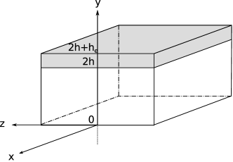
Figure 1: Sketch of the channel geometry. The interface between the channel region and the elastic medium is located at $y=2h$, while two solid rigid walls bounds the domain at $y=0$ and $2h+h_{e}$.

2 Formulation

We consider the turbulent flow of an incompressible viscous fluid through a channel with an incompressible hyper elastic wall. Figure 1 shows a sketch of the geometry and the Cartesian coordinate system, where $x$, $y$ and $z$ ($x_{1}$, $x_{2}$, and $x_{3}$) denote the streamwise, wall-normal and spanwise coordinates, while $u$, $v$ and $w$ ($u_{1}$, $u_{2}$, and $u_{3}$) denote the respective components of the velocity vector field. The upper interface is initially located at $y=2h$, while the lower and upper impermeable walls are located at $y=0$ and $2h+h_{e}$, respectively. Hence, $h_{e}$ represents the height of the hyper-elastic layer.

The fluid and solid phase motion is governed by conservation of momentum and the incompressibility constraint:

$$\frac{\partial u_{i}^{f}}{\partial t}+\frac{\partial u_{i}^{f}u_{j}^{f}}{\partial x_{j}} =\frac{1}{\rho}\frac{\partial\sigma_{ij}^{f}}{\partial x_{j}},$$ (1a)

$$\frac{\partial u_{i}^{f}}{\partial x_{i}} =0,$$ (1b)

$$\frac{\partial u_{i}^{s}}{\partial t}+\frac{\partial u_{i}^{s}u_{j}^{s}}{\partial x_{j}} =\frac{1}{\rho}\frac{\partial\sigma_{ij}^{s}}{\partial x_{j}},$$ (1c)

$$\frac{\partial u_{i}^{s}}{\partial x_{i}} =0,$$ (1d)

where the suffixes ^f and ^s are used to indicate the fluid and solid phase. In the previous set of equations, $\rho$ is the density (assumed to be the same for the solid and fluid), and $\sigma_{ij}$ the Cauchy stress tensor. The kinematic and dynamic interactions between the fluid and solid phases are determined by enforcing the continuity of the velocity and traction force at the interface between the two phases

$$u_{i}^{f} =u_{i}^{s},$$ (2a)

$$\sigma_{ij}^{f}n_{j} =\sigma_{ij}^{s}n_{j},$$ (2b)

where $n_{i}$ denotes the normal vector at the interface.

To numerically solve the fluid-structure interaction problem at hand, we use the so called one-continuum formulation (Tryggvason et al., 2007), where only one set of equations is solved over the whole domain. This is achieved by introducing a monolithic velocity vector field $u_{i}$ valid everywhere; this is found by applying the volume averaging procedure (Takeuchi et al., 2010; Quintard & Whitaker, 1994) and reads

$$u_{i}=\left(1-\phi^{s}\right)u_{i}^{f}+\phi^{s}u_{i}^{s},$$ (3)

where $\phi^{s}$ is the solid volume fraction. This is zero in the fluid, $\phi^{s}=0$, whereas $\phi^{s}=1$ in the solid, with $0\leq\phi^{s}\leq 1$ close to the interface. In particular, the isoline at $\phi^{s}=1/2$ represents the interface. Similarly to the Volume of Fluid (Hirt & Nichols, 1981) and Level Set (Sussman et al., 1994; Chang et al., 1996) methods used to simulate multi phase flows, we can write the stress in a mixture form as

$$\sigma_{ij}=\left(1-\phi^{s}\right)\sigma_{ij}^{f}+\phi^{s}\sigma_{ij}^{s}.$$ (4)

The fluid is assumed to be Newtonian so that the stress in the fluid

$$\sigma_{ij}^{f}=-p\delta_{ij}+2\mu^{f}D_{ij},$$ (5)

where $p$ is the pressure, $\mu^{f}$ the fluid dynamic viscosity, $D_{ij}$ the strain rate tensor defined as

$$D_{ij}=\frac{1}{2}\left(\frac{\partial u_{i}}{\partial x_{j}}+\frac{\partial u_{j}}{\partial x_{i}}\right),$$ (6)

and $\delta$ is the Kronecker delta. The solid is an incompressible viscous hyper-elastic material undergoing only the isochoric motion with constitutive equation

$$\sigma_{ij}^{s}=-p\delta_{ij}+2\mu^{s}D_{ij}+\sigma_{ij}^{sh},$$ (7)

where $\mu^{s}$ is the solid dynamic viscosity, and the last term the hyper-elastic contribution modelled as a neo-Hookean material, thus satisfying the incompressible Mooney-Rivlin law. The constitutive equation for the solid becomes

$$\sigma_{ij}^{s}=-p\delta_{ij}+2\mu^{s}D_{ij}+GB_{ij}$$ (8)

where $B_{ij}$ is the left Cauchy-Green deformation tensor, and $G$ the modulus of transverse elasticity. The solid constitutive equation is a function of the left Cauchy-Green deformation tensor, and the set of equations for the solid material can be closed in a purely Eulerian manner by updating its component with the following transport equation:

$$\frac{\partial B_{ij}}{\partial t}+\frac{\partial u_{k}B_{ij}}{\partial x_{k}}=B_{kj}\frac{\partial u_{i}}{\partial x_{k}}+B_{ik}\frac{\partial u_{j}}{\partial x_{k}}.$$ (9)

The previous equation comes from the fact that the upper convected derivative of the left Cauchy-Green deformation tensor is identically zero (Bonet & Wood, 1997). To close the full system, one transport equation is needed for the solid volume fraction $\phi^{s}$,

$$\frac{\partial\phi^{s}}{\partial t}+\frac{\partial u_{k}\phi^{s}}{\partial x_{k}}=0.$$ (10)

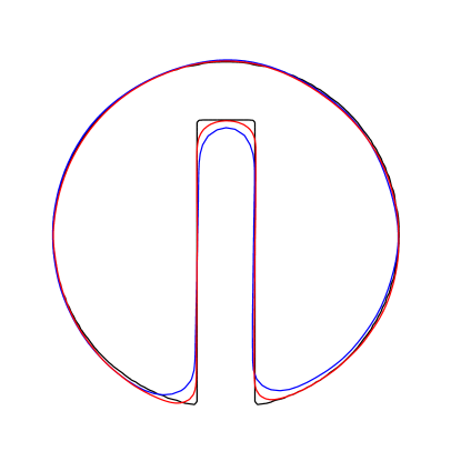
Figure 2: The Zalesak’s disk: validation of the current implementation by simulating a slotted disc undergoing solid body rotation, see Zalesak (1979). The black line denotes the exact solution, whereas blue and red the solution obtained with $64$ and $128$ grid points per diameter.

2.1 Numerical implementation

In order to simulate the elastic material, we follow the method for fluid-structure interaction problems recently developed by Sugiyama et al. (2011). These authors propose a fully Eulerian formulation on a fixed Cartesian grid based on a one-continuum formulation where the two phases are distinguished using an indicator function.

The time integration method used to solve equations (1), (9), and (10) is based on a explicit fractional-step method (Kim & Moin, 1985), where all the terms are advanced with the third order Runge-Kutta scheme, except the solid hyper-elastic contribution which is advanced with Crank-Nicolson (Min et al., 2001). At each time step the volume fraction $\phi^{s}$ and left Cauchy-Green deformation tensor $B_{ij}$ are updated first

$$\frac{\phi^{k}-\phi^{k-1}}{\Delta t} +\beta^{k}\left(\frac{\partial u_{k}\phi}{\partial x_{k}}\right)^{k-1}+\gamma^{k}\left(\frac{\partial u_{k}\phi}{\partial x_{k}}\right)^{k-2}=0,$$ (11a)

$$\begin{split}\frac{B_{ij}^{k}-B_{ij}^{k-1}}{\Delta t}&+\beta^{k}\left(\frac{\partial u_{k}B_{ij}}{\partial x_{k}}-B_{kj}\frac{\partial u_{i}}{\partial x_{k}}-B_{ik}\frac{\partial u_{j}}{\partial x_{k}}\right)^{k-1}+\\ &+\gamma^{k}\left(\frac{\partial u_{k}B_{ij}}{\partial x_{k}}-B_{kj}\frac{\partial u_{i}}{\partial x_{k}}-B_{ik}\frac{\partial u_{j}}{\partial x_{k}}\right)^{k-2}=0,\end{split}$$ (11b)

followed by the prediction step of the momentum conservation equations

$$\begin{split}\frac{u_{i}^{*}-u_{i}^{k-1}}{\Delta t}&+2\alpha^{k}\frac{1}{\rho}\frac{\partial p^{(k-1)}}{\partial x_{i}}+\alpha^{k}\left(-\frac{1}{\rho}\frac{\partial\sigma^{sh}_{ij}}{\partial x_{j}}\right)^{k}+\alpha^{k}\left(-\frac{1}{\rho}\frac{\partial\sigma^{sh}_{ij}}{\partial x_{j}}\right)^{k-1}+\\ &+\beta^{k}\left(\frac{\partial u_{i}u_{j}}{\partial x_{j}}-\frac{1}{\rho}\frac{\partial\sigma^{\prime}_{ij}}{\partial x_{j}}\right)^{k-1}+\gamma^{k}\left(\frac{\partial u_{i}u_{j}}{\partial x_{j}}-\frac{1}{\rho}\frac{\partial\sigma^{\prime}_{ij}}{\partial x_{j}}\right)^{k-2}=0.\end{split}$$ (12)

In the previous equations, $\Delta t$ is the overall time step from $t^{n}$ to $t^{n+1}$, the superscript ^∗ is used for the predicted velocity, while the superscript ^k denotes the Runge-Kutta substep, with $k=0$ and $k=3$ corresponding to time $n$ and $n+1$.

The pressure equation that enforces the solenoidal condition on the velocity field is solved via a Fast Poisson Solver

$$\frac{\partial\psi^{k}}{\partial x_{i}\partial x_{i}}=\frac{\rho}{2\alpha^{k}\Delta t}\frac{\partial u_{i}^{*}}{\partial x_{i}},$$ (13)

and, finally, the pressure and velocity are corrected according to

$$p^{k} =p^{k-1}+\psi^{k},$$ (14a)

$$u_{i}^{k} =u_{i}^{*}-2\alpha^{k}\frac{\Delta t}{\rho}\frac{\partial\psi^{k}}{\partial x_{i}},$$ (14b)

where $\psi$ is the projection variable, and $\sigma_{ij}^{\prime}$ is the deviatoric stress tensor. $\alpha$, $\beta$, and $\gamma$ are the integration constants, whose values are

$$\begin{array}[]{ccc}\alpha^{1}=\frac{4}{15}&\alpha^{2}=\frac{1}{15}&\alpha^{3}=\frac{1}{6}\\ \\ \beta^{1}=\frac{8}{15}&\beta^{2}=\frac{5}{12}&\beta^{3}=\frac{3}{4}\\ \\ \gamma^{1}=0&\gamma^{2}=-\frac{17}{60}&\gamma^{3}=-\frac{5}{12}\end{array}$$ (15)

The governing differential equations are solved on a staggered grid using a second order central finite-difference scheme, except for the advection terms in equation (11) where the fifth-order WENO scheme is applied, as it was proved to work properly by Sugiyama et al. (2011). A comprehensive review on the properties of different numerical schemes for the advection terms is reported by Min et al. (2001).

The Zalesak’s disk (Zalesak, 1979), i.e., a slotted disc undergoing solid body rotation, is a standard benchmark to validate the numerical schemes for advection problems, since the initial shape should not deform under solid body rotation. The set-up is the same described by Zalesak (1979) and the comparison of the initial shape (black line) and that after one full rotation (red and blue lines) is shown in figure 2. Two grid resolutions are considered here, $64$ and $128$ grid points per diameter, shown in blue and red, respectively. The final shape of the disk shows an overall good agreement with the initial one, with better agreement on the finer grid. As expected, the major differences are located on the edges of the geometry.

Figure 3: (a)-(c) Comparison of the hyper-elastic solid deformation in the lid-driven cavity with published results. The solid line represents our results, while the dots are taken from Sugiyama et al. (2011). The different snapshots correspond to the time $t=2.34L/V_{w}$, $4.69L/V_{w}$, and $7.03L/V_{w}$. The color background contour is the magnitude of the velocity, and the color scale goes from $0$ (violet) to $1V_{w}$ (red). (d) Trajectories of the solid centroid in the lid-driven cavity in a time range $t\in\left[0,20L/V_{w}\right]$.

2.2 Code validation

The code has been validated by performing a full $2D$ Eulerian simulation of a deformable solid motion in a lid-driven square cavity of side $L$, at a Reynolds number of $Re=\rho V_{w}L/\mu=100$, where $V_{w}$ is the velocity of the moving top wall, and $\rho$ and $\mu$ the density and dynamic viscosity of both phases (i.e., $\rho=\rho^{s}=\rho^{f}$ and $\mu=\mu^{s}=\mu^{f}$). The system is initially at rest, and the initial solid shape is circular with a radius of $0.2L$, centered at $\left(0.6L,0.5L\right)$. The solid phase is neo-Hookean material with modulus of transverse elasticity $G=0.1\rho V_{w}^{2}$. The numerical domain is discretised with $512\times 512$ grid points.

Figure 3(a-c) visualizes the solid deformation at three different equispaced time instants, starting from $t=1.17L/V_{w}$ to $t=7.03L/V_{w}$. The solid lines represents the instantaneous particle shapes, while the dots are the results by Sugiyama et al. (2011). Further comparison is provided in figure 3(d), where we display the trajectory of the solid centroid for $t\in\left[0,20L/V_{w}\right]$ from our simulation (solid line) and that provided by Sugiyama et al. (2011). The particle shape and trajectory is in very good agreement with the published results. Note that, a comparison between this fully Eulerian procedure and a Lagrangian one is provided in Sugiyama et al. (2011), together with other validations and test cases.

2.3 Numerical details

For all the turbulent flows considered hereafter, the equations of motion are discretised by using $1296\times 540\times 648$ grid points on a computational domain of size $6h\times 2.5h\times 3h$ in the streamwise, wall-normal and spanwise directions. The spatial resolution has been chosen in order to properly resolve the wall deformation, satisfying the constraint $\Delta x^{w+}=\Delta y^{w+}=\Delta z^{w+}<0.8$. For the case at highest Reynolds number, a grid refinement study was performed using $1944\times 810\times 972$ grid points in the streamwise, wall-normal and spanwise directions ($50\%$ more in each direction). The difference in the resulting friction coefficient $C_{f}$ results to be less than $2\%$.

All the simulations are started from a fully developed turbulent channel flow with a perfectly flat interface between the fluid and solid phases. After the flow has reached statistical steady state, the calculations are continued for an interval of $600h/U_{b}$ time units, during which $120$ full flow fields are stored for further statistical analysis. To verify the convergence of the statistics, we have computed them using different number of samples and verified that the differences are negligible.

3 Results

Figure 4: Friction Reynolds number of the top deformable wall $Re_{\tau}$, as a function of the elastic modulus $G$. The coloured symbols blue, magenta, red, and green are used for the cases of decreasing elastic modulus $G$. The dashed horizontal line in the figure represents the value for the rigid wall case (Kim et al., 1987).

We study turbulent channel flows over viscous hyper-elastic walls, together with a baseline case over stationary impermeable walls taken by the seminal work of Kim et al. (1987). All the simulations are performed at constant flow rate, so that the flow Reynolds number based on the bulk velocity is fixed at $2800$, i.e., $Re=\rho U_{b}h/\mu^{f}=2800$, where the bulk velocity is the average value of the mean velocity computed across the whole domain occupied by the fluid phase. This choice facilitates the comparison between the flow in a channel with elastic walls and the flow in a channel bounded by rigid impermeable walls. In general, if the pressure gradient is kept constant in time, the flow rate oscillates in time around a constant value. On the other hand, if the flow rate is kept constant in time the pressure gradient oscillates around a constant value. In the present work, consistently with choosing $U_{b}$ as the characteristic velocity, we opt for enforcing the constant flow rate condition; hence the appropriate value for the instantaneous value of the streamwise pressure gradient is determined at every time step.

The elastic wall in the unstressed condition is flat and parallel to the bottom rigid wall, and its reference height is fixed to $h_{e}=0.5h$. The modulus of transverse elasticity $G$ is varied and four values are considered here, ranging from an almost rigid case, $G=2.0\rho U_{b}^{2}$, to a highly elastic one, $G=0.25\rho U_{b}^{2}$. The viscosity of the solid is set equal to the fluid one, i.e., $\mu^{s}=\mu^{f}=\mu$, except for the results in the last section, section 3.4, where we report data for two solid materials with larger and lower viscosities. In particular, the viscosity ratio $\mu^{s}/\mu^{f}$ is set equal to $0.1$ and $10$. The full set of simulations is reported in table 1, together with some mean quantities, such as the resulting friction Reynolds number based on the bottom rigid wall $Re_{\tau}^{w}$ and based on the top elastic wall $Re_{\tau}$, the maximum velocity $\overline{u}_{M}$, and its $y$-coordinate location $y_{M}$. The friction Reynolds number $Re_{\tau}$ is also shown in figure 4 as a function of the elastic modulus $G$.

Case	$h_{e}/h$	$\mu^{s}/\mu^{f}$	$G/\left(\rho U_{b}^{2}\right)$	$Re_{\tau}^{w}$	$Re_{\tau}$	$\overline{u}_{M}/U_{b}$	$y_{M}/h$
Reference	$-$	$-$	$-$	$178.5$	$178.5$	$1.16$	$0.000$
$G\downarrow$	$0.5$	$1$	$4.0$	$179.0$	$180.8$	$1.17$	$-0.030$
$G\downarrow\downarrow$	$0.5$	$1$	$2.0$	$182.1$	$203.3$	$1.19$	$-0.076$
$G\downarrow\downarrow\downarrow$	$0.5$	$1$	$1.0$	$193.0$	$240.5$	$1.23$	$-0.206$
$G\downarrow\downarrow\downarrow\downarrow$	$0.5$	$1$	$0.5$	$202.3$	$307.0$	$1.32$	$-0.386$
$\mu^{s}\downarrow$	$0.5$	$0.1$	$1.0$	$192.9$	$240.4$	$1.22$	$-0.197$
$\mu^{s}\uparrow$	$0.5$	$10.$	$1.0$	$187.0$	$226.0$	$1.19$	$-0.127$

Table 1: Summary of the DNSs performed at different viscous hyper-elastic parameters, all at a fixed bulk Reynolds number equal to $Re=2800$.

Viscous units, used above to express spatial resolution, will be often employed in the following; they are indicated by the superscript ⁺, and are built using the friction velocity $u_{\tau}$ as velocity scale and the viscous length $\delta_{\nu}=\nu/u_{\tau}$ as length scale. For a turbulent channel flow with solid walls, the dimensionless friction velocity is defined as

$$u_{\tau}=\sqrt{\dfrac{1}{Re}\left.\dfrac{d\overline{u}}{dy}\right|_{y=0}},$$ (16)

where $\overline{u}$ is the mean velocity, and the subscript indicates that the derivative is taken at $y=0$, the location of the solid wall. When the channel has moving walls, the definition (16) must be modified to account for the turbulent shear stresses that are in general non-zero at the solid-fluid interface. Similarly to what usually done for porous walls (Breugem et al., 2006), we define

$$u_{\tau}=\sqrt{\dfrac{1}{Re}\left.\dfrac{d\overline{u}}{dy}\right|_{y=2}-\left.\overline{u^{\prime}v^{\prime}}\right|_{y=2}},$$ (17)

where $\overline{u^{\prime}v^{\prime}}$ is the off-diagonal component of the Reynolds stress tensor and the quantities are evaluated at the mean interface location, $y=2$. In our simulations two viscous units can be defined, one based on the bottom rigid wall, and one on the top elastic wall, by using equation (16) and equation (17). In the following, we will distinguish the two units adding a superscript ^w when referring to the bottom rigid wall. The actual value of the friction velocity of the elastic wall is computed from its friction coefficient, found by combining the information of the total $C_{f}$, obtained from the driving streamwise pressure gradient, and the one of the lower rigid wall found by equation (16).

3.1 Mean flow

Figure 5(a) shows the mean velocity profile $\overline{u}$ as a function of the wall-normal coordinate. The black $+$ symbol is used for the reference case with rigid walls taken from Kim et al. (1987), and reproduced with the same code in Picano et al. (2015); the solid lines indicate the results from the present simulations with blue, magenta, red, and green used for cases with increasing elasticity (lower transverse elastic modulus $G$). This color scheme will be used through the whole paper. The presence of one rigid and one elastic wall makes the mean velocity profile skewed, with its maximum $\overline{u}_{M}$ increasing and located closer to the bottom wall as the elasticity increases. Note that the mean velocity of the elastic wall is equal to zero.

Figure 5: (a) Comparison of the streamwise mean velocity profile $U$ of a turbulent channel flow at $Re=2800$ over rigid walls ($+$ symbols) and over different hyper-elastic walls (solid lines). The blue, magenta, red, and green lines are used for the cases $G\downarrow$, $G\downarrow\downarrow$, $G\downarrow\downarrow\downarrow$, and $G\downarrow\downarrow\downarrow\downarrow$, respectively, i.e., for increasing elasticity (lower transverse elastic modulus $G$). The results for the rigid case are taken from Kim et al. (1987). (b) Mean velocity profile $U$ versus the distance from the bottom rigid wall in wall units.

Figure 5(b) shows the mean velocity profiles versus the logarithm of the distance from the bottom rigid wall in wall-units. For the turbulent channel flows over rigid impermeable walls (shown with the symbol $+$), we can usually identify three regions: firstly, the viscous sublayer for $y^{w+}<5$ where the variation of $\overline{u}^{w+}$ with $y^{w+}$ is approximately linear, i.e.,

$$\overline{u}^{w+}=y^{w+}.$$ (18)

In the so-called log-law region, $y^{w+}>30$ the variation of $\overline{u}^{w+}$ versus $y^{w+}$ is logarithmic, i.e.,

$$\overline{u}^{w+}=\dfrac{1}{k}\log y^{w+}+B,$$ (19)

defined by the coefficients $k$ (the von Karman constant) and $B$. The values of $k$ and $B$ for smooth rigid walls are usually assumed to be $k=0.41$ and $B=5$. However, for the Reynolds number that we are considering, a better fit with experimental and numerical simulations is obtained with $k=0.40$ and $B=5.5$. Finally, the region between $5$ and $30$ wall units is called buffer layer and neither laws hold.

As shown in figure 5(b), the velocity profiles from the cases with an elastic wall still coincide, which indicates that the scaling of the mean flow near the bottom wall is not altered by the presence of the deformable top wall, the only differences being a reduced inertial range and the location of the maximum velocity at lower wall-distances due to the skewness of the mean velocity profile.

Case	$d/h$	$k+\Delta k$	$\Delta U^{+}$	$\delta/h$	$\delta^{\prime}/h$
Reference	$-$	$0.41$	$-$	$-$	$-$
$G\downarrow$	$0.011$	$0.36$	$1.5$	$0.011$	$0.003$
$G\downarrow\downarrow$	$0.069$	$0.29$	$7.5$	$0.061$	$0.007$
$G\downarrow\downarrow\downarrow$	$0.120$	$0.25$	$14.5$	$0.095$	$0.025$
$G\downarrow\downarrow\downarrow\downarrow$	$0.193$	$0.20$	$24.4$	$0.126$	$0.042$
$\mu^{s}\downarrow$	$0.120$	$0.25$	$14.5$	$0.090$	$0.015$
$\mu^{s}\uparrow$	$0.055$	$0.31$	$7.9$	$0.054$	$0.008$

Table 2: Summary of the log-law fitting parameters and wall deformations for the cases shown in table 1. The table provides the origin shift $d$, the modified von Karman constant $k+\Delta k$, the shift of the velocity profile $\Delta U^{+}$, the maximum and root mean square values of the wall deformation $\delta$ and $\delta^{\prime}$.

Figure 6: (a) Mean velocity profile $U$ versus the distance from the top rigid wall $\tilde{y}+d$ in wall units, and (b) $(\tilde{y}+d)^{+}d\overline{u}^{+}/d\tilde{y}^{+}$ as a function of $\tilde{y}^{+}$ for the case $G\downarrow\downarrow$. The three lines in (b) correspond to three values of $d$, i.e., $0.00$ (solid line), $0.07$ (dashed line), and $0.14$ (dash-dotted line). The colour scheme is the same as in figure 5.

The mean velocity profiles in inner units based on the friction at the top moving walls are shown in figure 6(a). Differently from figure 5(b), the profiles are plotted versus $\tilde{y}+d=(2h-y)+d$, where $d$ is a shift of the origin. This shift was introduced by Jackson (1981) for rough walls and then used by Breugem et al. (2006) for permeable walls. Introducing $d$, the log-law is modified as

$$\overline{u}^{+}=\dfrac{1}{\lambda}\log\frac{\tilde{y}+d}{y_{0}},$$ (20)

where $\lambda$ is the slope of the inertial range, which may differ from $k$, i.e., $\lambda=k+\Delta k$, and $y_{0}$ is the so-called equivalent roughness height. Through simple manipulation, the previous relation can be rewritten as

$$\overline{u}^{+}=\dfrac{1}{\lambda}\log\left(\tilde{y}+d\right)^{+}-\frac{1}{\lambda}\log y_{0}^{+},$$ (21)

and for a better comparison with equation (19) as

$$\overline{u}^{+}=\dfrac{1}{k+\Delta k}\log\left(\tilde{y}+d\right)^{+}+B-\Delta U^{+}.$$ (22)

In order to identify the value of $d$, we have first plot $(\tilde{y}+d)^{+}d\overline{u}^{+}/d\tilde{y}^{+}$ as a function of $\tilde{y}^{+}$ for several values of $d$. Inside the logarithmic layer this quantity must be constant and equal to the inverse of the slope in the inertial range, i.e., $1/\left(k+\Delta k\right)$. In this way, the correct value of the shift can be identified as the one providing a region with constant $(\tilde{y}+d)^{+}d\overline{u}^{+}/d\tilde{y}^{+}$ (an equilibrium range). The procedure is exemplified in figure 6(b) where we report $(\tilde{y}+d)^{+}d\overline{u}^{+}/d\tilde{y}^{+}$ for the case $G\downarrow\downarrow$ and three values of $d$, i.e., $0.00$ (solid line), $0.07$ (dashed line), and $0.14$ (dash-dotted line). Note that the slope in the inertial range is slightly positive for $d=0.0$, while it becomes negative for $d=0.14$; only for the correct value $d=0.07$ the slope is null, providing $k+\Delta k=0.294$. Once $d$ and $\Delta k$ are known, $\Delta U^{+}$ can be found by a simple fitting.

This procedure has been repeated for all the cases, obtaining the values of the fitting parameters reported in table 2 and used for the scaling in figure 6(a); note that the dashed lines reported in the figure are computed using these values. All the cases with elastic walls under consideration show an increase in the slope of the logarithmic region, $\Delta k<0$, when compared with the flow over rigid walls, as well as a downward shift $\Delta U^{+}$. The change of slope in the logarithmic region, corresponding to an increase of drag, was also found in turbulent channel flow over porous walls by Breugem et al. (2006) for high values of permeabilities, while no change was found for low values of permeability in Rosti et al. (2015) and for the turbulent channel flow over rough walls by Orlandi & Leonardi (2008); indeed the only effect of a rough wall was a downward shift of the mean profile, also associated to a drag increase.

As discussed by Orlandi & Leonardi (2008), previous studies employing Direct Numerical Simulations with different boundary conditions for the three velocity components at the wall have shown that the turbulent flow is strongly linked to the fluctuations of the wall-normal velocity component $v^{\prime}$, with rms values denoted by a ^′ in the following. This has been shown by Orlandi et al. (2003) for the case of a rough surface made of two-dimensional square bars that can be mimicked by distributions of $v^{\prime}$, by Flores & Jimenez (2006) who used synthetic velocity distributions, and by Jimenez et al. (2001) who modelled a permeable wall adding a transpiration boundary condition proportional to the local pressure fluctuations $p^{\prime}$, i.e., $v=-\beta p^{\prime}$, $\beta$ being a constant. Also, Cheng & Castro (2002) experimentally showed that the roughness function correlates well with $v^{\prime}$. Based on these previous data, Orlandi & Leonardi (2006, 2008) proposed first a correlation between $\Delta U^{+}$ and $v^{\prime}$, then improved by using $v^{\prime+}$, finally showing that

$$\Delta U^{+}\approx\frac{B}{k}v^{\prime+}.$$ (23)

Figure 7: (a) Rms values of velocity fluctuations at the interface, as function of the inverse of the elastic modulus ($\rho U_{b}^{2}/G$). The solid line is used for the streamwise component, the dashed line for the wall-normal component, and the dash-dotted one for the spanwise component. (b) Rms of the wall-normal velocity component $v^{\prime}$ versus the velocity shift $\Delta U^{+}$, see equation (24). The black circles are the data for the turbulent channel flow over porous wall investigated by Breugem et al. (2006). The colour scheme is the same as in figure 5.

These correlation was validated against the results by Orlandi et al. (2003); Orlandi & Leonardi (2006, 2008); Flores & Jimenez (2006), and Cheng & Castro (2002). Both numerical and experimental data fit well with relationship (23) for values of $v^{\prime+}$ up to $0.8$; above this values the linear correlation departs from the data, showing hence discrepancies at high $v^{\prime+}$.

In order to test a similar correlation also for the present configuration, we display the rms of the velocity fluctuation components at the mean interface location, $y=2h$, versus the elasticity $\rho U_{b}^{2}/G$ in figure 7(a). In the picture, the solid, dashed and dash-dotted lines are used for the streamwise, wall-normal and spanwise velocity components. All the three components of the fluctuating velocity appear to vary almost linearly with the inverse of the elasticity, the wall-normal component of the velocity being the fastest and the spanwise the slowest. Figure 7(b) shows the log-law shift $\Delta U^{+}$ as a function of the ratio between the wall-normal velocity fluctuation $v^{\prime}$ and the change of the inertial range slope $\Delta k$. For all the cases considered, we find that a linear relation well approximates the two quantities, i.e.,

$$\Delta U^{+}\approx\frac{v^{\prime}}{\Delta k}.$$ (24)

The proposed fit, given in equation (24), is here tested also for the case of a turbulent channel flow over porous wall by using the data of the simulations in Breugem et al. (2006), shown in figure 7(b) as black circles. Interestingly, the agreement is quite good also in this case (please note, that the values of $\Delta U^{+}$ and $v^{\prime}$ are not reported but extracted from the figures).

3.2 Velocity fluctuations

Figure 8: Wall-normal profiles of the different components of the Reynolds stress tensor, normalised with $U_{b}^{2}$ for a turbulent channel flow over hyper-elastic walls. The symbols indicate the flow between two rigid walls from Kim et al. (1987). Panels (a), (b), and (c) show the diagonal components $u^{\prime}u^{\prime}$, $v^{\prime}v^{\prime}$, and $w^{\prime}w^{\prime}$, while (d) the cross term $u^{\prime}v^{\prime}$. The colour scheme is the same as in figure 5.

We continue our comparison between the turbulent channel flows with rigid and elastic walls by analyzing the wall-normal distribution of the diagonal component of the Reynolds stress tensor; these are shown in 8(a-c) together with the data from Kim et al. (1987) for the rigid case. All the components are strongly affected by the moving wall, and the effect is not limited to the region close to the interface, but it extends also beyond the centreline. The peaks of the Reynolds stresses move farther from the walls as the elasticity is increased. As already showed in figure 7(a), all the components have non-zero values at $y=2h$ for the elastic cases, since the no-slip condition is now enforced on a wall which is moving, i.e., $u_{i}^{f}=u_{i}^{s}$. The Reynolds stress components decrease inside the solid layer, eventually becoming zero at the rigid top wall, located at $y=2.5h$. Note that for the most elastic case considered ($G\downarrow\downarrow\downarrow\downarrow$) all the stress components, especially the wall-normal one, do not clearly vanish until reaching the rigid top wall, thus indicating that the fluctuations propagate deeply inside the solid layer. In relative terms, the spanwise and wall-normal components are the most affected by the wall elasticity, which can be attributed to a weakening of the wall-blocking and wall-induced viscous effects (Perot & Moin, 1995a, b), and observed also in the experiments of Krogstad et al. (1992) and Krogstadt & Antonia (1999) on boundary-layer flows over rough walls. The wall-normal component displays a secondary peak very close to the interface, which grows with the elasticity and eventually becomes its maximum value. This secondary peak is associated with the oscillatory movement of the wall. Indeed, the dashed line in figure 8(b) connects the maximum of the wall-normal oscillation amplitude $\delta/h$ reported in table 2 with the local value of the Reynolds stress, thus, clearly showing that the location of the peak coincides with the maximum oscillation of the wall. We also note that the peak of the streamwise component of the fluctuating velocity, $u^{\prime 2}$, grows much less then that pertaining the other two components. This increase is even lower than the growth of the friction Reynolds number, corresponding to a reduction in wall units. The reduced amplitude of the streamwise fluctuations is usually associated with the absence or reduction of streaky structures above a wall (Rosti et al., 2015; Breugem et al., 2006), which is true also in the present case, as shown in the next section.

Finally, figure 8(d) depicts the wall-normal profile of the off-diagonal component of the Reynolds stress tensor. Also this cross component is strongly affected by the presence of the moving wall. In particular, the maximum value increases and moves away from the wall as the elasticity increases. Consequently, also the location where the stress is zero $y_{uv}$, i.e., zero turbulent production, moves closer to the bottom solid walls, from $y=1h$ for the rigid case to $y\approx 0.58h$ for the most elastic upper wall. Nevertheless the stress profiles vary linearly between the two peaks, of opposite sign, close to each wall, although with different slopes. At the interface the value of the stress is not null as in the rigid case, however, inside the elastic layer the stress vanishes quickly.

Figure 9: Wall-normal profiles of the turbulent kinetic energy $\mathcal{K}=\left(u^{\prime 2}+v^{\prime 2}+w^{\prime 2}\right)/2$, normalised with the friction velocities of (a) the bottom rigid wall $u_{\tau}^{w}$ and (b) of the top elastic wall $u_{\tau}$. Symbols indicate the flow between two rigid walls from the data in Kim et al. (1987). The colour scheme is the same as in figure 5.

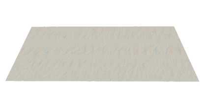
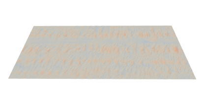
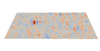
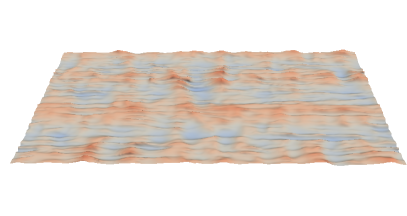
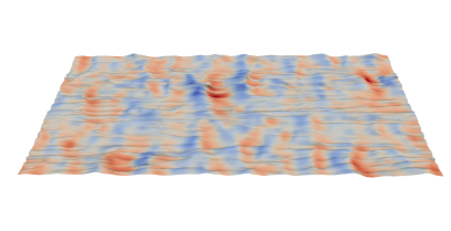
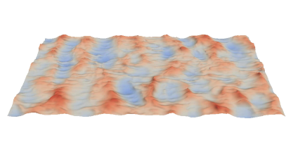
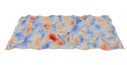
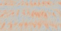
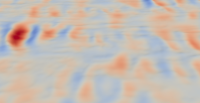
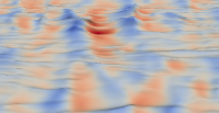
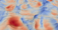
Figure 10: Instantaneous configuration of the top elastic wall, with transverse elastic modulus $G$ decreasing from top to bottom. The flow goes from left to right. The surfaces are coloured by the wall-normal distance on the left column, with the color scale ranging from $-0.13h$ (blue) to $0.13h$ (red), and by the pressure on the right column, with the color scale ranging from $-1\rho U_{b}^{2}$ (blue) to $1\rho U_{b}^{2}$ (red). The bottom row is a zoomed view of pictures on the left column.

An overall view of the velocity fluctuations can be inferred considering the turbulent kinetic energy $\mathcal{K}=\left(u^{\prime 2}+v^{\prime 2}+w^{\prime 2}\right)/2$, shown in figure 9. We display in figure 9(a) the kinetic energy normalised by the friction velocity $u_{\tau}^{w}$ at the bottom rigid wall as a function of the wall-normal distance $y/h$. As usual, the symbols represent the profiles from the DNS of Kim et al. (1987) of turbulent flow between two solid rigid walls. Close to the bottom wall the profiles coincide, as expected, which indicates that the influence of the moving wall on the velocity fluctuations near the other wall is negligible. In the boundary layer close to the moving wall, instead, we observe a strong increase of the kinetic energy, with the maximum value becoming the double of the peak close to the bottom wall. Figure 9(b) reports the same turbulent kinetic energy profiles, but now normalized by the friction velocity $u_{\tau}$ at the moving top wall. Except for the case $G\downarrow\downarrow\downarrow\downarrow$, the profiles tend to coincide away from the wall (for $y$ in the range between $1h$ and $1.8h$), whereas the peak close to the moving wall is slightly lower for higher wall elasticities. The reduced peak is mainly due to the weak increase (decrease in wall units) of the streamwise component of the velocity fluctuations discussed above. The inset in figure 9(b) shows again the turbulent kinetic energy profile close to the moving wall versus the wall normal distance $\tilde{y}$ divided by the coordinate $\tilde{y}_{uv}$ where the shear component of the Reynolds stress tensor cross zero. This scaling compensates for the asymmetry in the geometry, similarly to what done by Leonardi et al. (2007), and provides a better collapse of the profiles.

3.3 Solid deformation and flow structures

We now discuss in more details the deformation of the wall and its effect on the emerging flow coherent structures. Figure 10 shows one instantaneous configuration of the top elastic wall for the four cases considered here with growing elasticity from top to bottom, and with the flow from left to right. The wall surface is coloured by the wall-normal distance to the reference straight unstressed condition on the left column, with the color scale ranging from $-0.13h$ (blue) to $0.13h$ (red), and by the pressure on the right column, with the color scale ranging from $-1\rho U_{b}^{2}$ (blue) to $1\rho U_{b}^{2}$ (red). The wall surface deforms with a maximum amplitude of the wall deformation $\delta$ ranging approximately from $1\%$ of the channel half height $h$ for the most rigid case ($G\downarrow$) to $13\%$ in the most deformable one ($G\downarrow\downarrow\downarrow\downarrow$). We recall that the values of $\delta$ are reported in table 2, together with the root mean square value of the wall deformation $\delta^{\prime}$. It is interesting to note that the spanwise coherency of the wall deformation tends to increase as $G$ is decreased, i.e., the deformation increases.

Figure 11: Profiles of the (a) streamwise $\sigma_{11}^{sh}$ and (b) cross $\sigma_{12}^{sh}$ hyper-elastic stress tensor components as a function of the wall-normal coordinate $y/h$ for the different values of the transverse elastic modulus $G$ under investigation. The colour scheme is the same as in figure 5.

Figure 11 shows the mean profile of the hyper-elastic stress tensor streamwise $\sigma_{11}^{sh}$ and shear $\sigma_{12}^{sh}$ components (see equation (8)). We note that the mean streamwise component is zero in the fully fluid region ($y>2h-\delta$) and rapidly grows for $2h-\delta<y<2h+\delta$, before reaching its positive maximum value at the solid wall, $y=2.5h$. The shear component follows a similar trend, but has a maximum negative value at the wall, with the shear component being one or two order of magnitude smaller then the streamwise one. While $\sigma_{11}^{sh}$ decreases as $G$ is reduced, i.e., for higher wall elasticity, on the contrary, $\sigma_{12}^{sh}$ increases (in absolute value). Note also that the values of the stress components approximately scale with $G$.

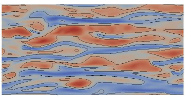
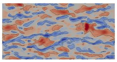
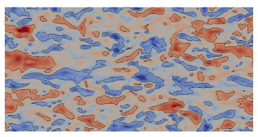
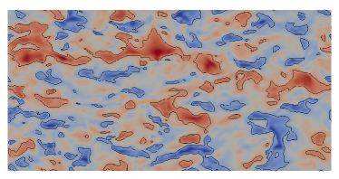
Figure 12: Instantaneous contour of the streamwise velocity fluctuations $u^{\prime}$ on the $x-z$ plane at $\left(\tilde{y}+d\right)^{+}=10$ for walls with transverse elastic modulus $G$ decreasing from top-left to bottom-right. The color scale goes from $-0.35U_{b}$ (blue) to $0.35U_{b}$ (red). The black lines represent the levels $u^{\prime+}\pm 4$.

The wall deformation affects the near-wall structure of the flow and this is visually confirmed by figure 12 that depicts the flow in the wall-parallel $x-z$ plane at $\left(\tilde{y}+d\right)^{+}=10$. The figure reports instantaneous contours of the streamwise velocity fluctuations $u^{\prime}$ with color scale from $-0.35U_{b}$ (blue) to $0.35U_{b}$ (red). In the same figure, we also show the levels $u^{\prime+}=\pm 4$ using black line contours. The goal of this figure is to identify the large-scale low- and high-speed near-wall streaks and show how they are affected by the wall elasticity. It is evident that the structures appear less elongated and more fragmented. Indeed, the flow is rich of small-scale features, consistent with a picture where the larger coherent structures are being broken into smaller pieces as a result of the wall movement. Figure 13 reports the same quantity but further from the wall, over the wall-parallel plane at $\tilde{y}=0.15h$. As for the near-wall structures the low- and high-speed streaks become shorter the more elastic the walls. Another interesting flow feature can be inferred by this figure, i.e., as the structure become shorter they also increase their spanwise size, eventually extending almost over the entire spanwise extent of our domain (see figure 13(d)), consistently with our previous discussion about the wall deformation (see figure 10(d)). These visual observations will be now quantified statistically by analysing the autocorrelation functions.

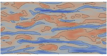
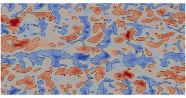
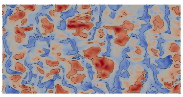
Figure 13: Instantaneous contour of the streamwise velocity fluctuations $u^{\prime}$ on the wall-parallel $x-z$ plane at $\tilde{y}=0.15h$ for walls with transverse elastic modulus $G$ decreasing from top-left to bottom-right. The color scale goes from $-0.35U_{b}$ (blue) to $0.35U_{b}$ (red). The black lines represent the levels $u^{\prime+}\pm 4$.

Figure 14: Line and colour contours of the one-dimensional autocorrelation of the (top) streamwise, (middle) wall-normal, and (bottom) spanwise velocity fluctuations as a function of the streamwise spacing $x/h$ for different $y$ coordinates, shown across half elastic wall and half channel. The thick and thin lines correspond to positive and negative values, ranging from $-0.1$ to $0.9$ with a step of $0.2$ between two neighbouring lines. The color scale ranges from $-0.1$ (white) to $1.0$ (black).

We now focus on the two-point correlation, defined as follows

$$R_{ii}(\bm{x},\bm{r})=\frac{\overline{u_{i}^{\prime}(\bm{x})u_{i}^{\prime}(\bm{x}+\bm{r})}}{\overline{u_{i}^{\prime 2}(\bm{x})}},$$ (25)

where the bar denotes average over time and homogeneous directions, and the prime the velocity fluctuation. Figure 14 illustrates the structure of the correlation functions along the streamwise direction $x$. These are one-dimensional correlations using the velocity difference along $x$, displayed for different $y$ coordinates across half of the elastic wall and the channel, i.e., for $y\in\left[1h,2.25h\right]$. For the most rigid wall, the correlations, and in particular that for the streamwise component $u$, present in the fluid region structures of relatively large length especially close to the walls. These are associated to the presence of elongated streaky structures that characterize the near-wall region. For a completely rigid wall, the streaks have typically a length of the order of $1000$ wall units, which would correspond to a correlation distance of roughly $5h$. As already seen in the visualisation in figure 12, the typical lengthscale is strongly reduced when increasing the wall elasticity, and indeed the correlation distance decreases significantly close to the wall, which is consistent with the reduction/absence of low- and high-speed streaks.

It is also interesting to note that the correlations change rapidly but continuously across the interface: the typical correlation length becomes much shorter for the $u$ component inside the elastic material as this cannot support streaky structures, while it remains comparable to the rigid-channel lengthscales for the other two velocity components. Inside the elastic wall, the correlations present an alternating sequence of progressively weaker negative and positive local peaks, a so-called cell-like pattern, associated to large-scale pressure fluctuations within the elastic material and just above the interface, as suggested by Breugem et al. (2006) for the flow over a porous wall. The typical wavelength of this oscillation for the most deformable case is approximately $1h$, thus corresponding to around $300$ plus units, a result consistent with the undulations shown in figure 12(d).

Figure 15: Line and colour contours of the one-dimensional autocorrelation of the (top) streamwise, (middle) wall-normal, and (bottom) spanwise velocity fluctuations as a function of the spanwise spacing $z/h$ for different $y$ coordinates, shown across half elastic wall and half channel. The thick and thin lines correspond to positive and negative values, ranging from $-0.1$ to $0.9$, with a step of $0.2$ between two neighbouring lines. The color scale ranges from $-0.1$ (white) to $1.0$ (black).

Finally, we consider the spanwise correlation functions for all three velocity components, see figure 15. On a rigid wall (Kim et al., 1987), the spanwise autocorrelation of the streamwise velocity component $u$ (figure 15(top)) exhibits a local minimum at $z^{w+}\approx 50$ in the region close to the wall, usually associated with the average spanwise distance between a low-speed and a neighbouring high-speed streak. Note that the periodicity of the streaks is deduced from the oscillations of the autocorrelation for larger spanwise spacings. The flow over elastic walls, conversely, display a larger correlation distance. Considering the wall-normal component of the velocity (figure 15(middle)), we observe a local minimum at roughly $y^{w+}\approx 25$ close to the rigid wall, which is consistent with the presence of quasi-streamwise vortices. The value of this local minimum decreases ($G\downarrow$ and $G\downarrow\downarrow$), and eventually disappear ($G\downarrow\downarrow\downarrow$ and $G\downarrow\downarrow\downarrow\downarrow$) in the case of moving elastic walls, suggesting that the quasi-streamwise vortices are strongly reduced. All the three velocity components present relatively large spanwise scales, and we thus find a statistical signature of the spanwise vortical structures or rolls similarly to those that have been identified in the turbulent flow over porous walls (Breugem et al., 2006; Rosti et al., 2015; Samanta et al., 2015), rough surfaces (Jimenez et al., 2001) and plant canopies (Finnigan, 2000). These structures are also believed to be the main cause of the performance loss of drag-reducing riblets when the riblets size is increased above their optimum (Garcia-Mayoral & Jimenez, 2011).

3.4 Effect of viscosity ratio

Figure 16: (a) Comparison of the streamwise mean velocity profile $U$ of a turbulent channel flow at $Re=2800$ over rigid walls ($+$ symbols) and over different hyper-elastic walls (red lines). The dotted, solid, and dashed lines are used for the cases $\mu^{s}/\mu^{f}=0.1$, $1.0$, and $10.0$ at a fixed elastic modulus $G=1.0$. The results for the rigid case are taken from Kim et al. (1987). (b) Mean velocity profile $U$ versus the distance from the top deformable wall in wall units.

We now consider the effect of the viscosity of the hyper-elastic material on the turbulence statistics for the case $G\downarrow\downarrow\downarrow$. Three viscosity ratios are examined, i.e., $\mu^{s}/\mu^{f}=0.1$, $1.0$, and $10.0$, see table 1 for a direct comparison of the values of the main global statistics.

When the elastic layer is less viscous than the fluid ($\mu^{s}\downarrow$), the friction Reynolds number is equal to $240$, same value obtained when the two viscosities are the same, while when the layer is more viscous than the fluid ($\mu^{s}\uparrow$), the Reynolds number decreases by $6\%$ to $226$. This trend is shown by the mean velocity profiles, reported in figure 16(a), where the dotted, solid, and dashed lines correspond to the flow with $\mu^{s}/\mu^{f}=0.1$, $1.0$, and $10.0$, respectively.

The mean velocity profile is less skewed in the high viscosity case ($\mu^{s}\uparrow$), with its maximum velocity $u^{M}$ decreasing and located closer to the centreline. The same velocity profiles are displayed versus the logarithm of the distance from the top wall in wall-units in figure 16(b). Again, the cases with $\mu^{s}<\mu^{f}$ and $\mu^{s}=\mu^{f}$ are almost undistinguishable, while the downward shift of the profile is reduced when $\mu^{s}<\mu^{f}$, moving the logarithmic part of the velocity profile towards that for a rigid wall. A similar picture emerges after examining other quantities, such the wall-normal profile of the Reynolds stress tensor components reported in figure 17.

Figure 17: Components of the Reynolds stress tensor as a function of the wall-normal coordinate $y$, normalised with the bulk velocity $U_{b}$ for a turbulent channel flow over a hyper-elastic wall. Symbols are for the rigid case from Kim et al. (1987) while the dotted, solid, and dashed lines are used for the cases $\mu^{s}/\mu^{f}=0.1$, $1.0$, and $10.0$ at a fixed elastic modulus $G=1.0$. The first three panels (a), (b), and (c) show the diagonal components $u^{\prime}u^{\prime}$, $v^{\prime}v^{\prime}$, and $w^{\prime}w^{\prime}$, whereas the cross term $u^{\prime}v^{\prime}$ is depicted in (d).

Overall, the results suggest that the behaviour of the flow in the limit of large and small values of $\mu^{s}$ and $G$ is different. Indeed, as $G$ or $\mu^{s}/\mu^{f}$ tend to infinity, the wall deformation decreases and the flow approaches the one over a rigid wall. On the contrary, while $G$ tending to $0$ increases the wall deformation, thus enhancing the turbulence, the flow appears to be almost unaffected by a decrease of $\mu^{s}/\mu^{f}$ below unity. Indeed, this behaviour suggests that when the viscosity ratio is low, the deformation is determined by the fluid fluctuations, while when the ratio $\mu^{s}/\mu^{f}$ is high the deformation is limited by the properties of the elastic layer.

4 Conclusion

We have carried out a number of direct numerical simulations of turbulent channel flow over a viscous hyper-elastic wall. The flow inside the fluid region is described by the Navier-Stokes equations, while momentum conservation and incompressibility are imposed inside the solid layer. The two sets of equations are coupled using a one-continuum formulation allowing a fully Eulerian description of the multiphase flow problem. We collect statistics by varying the values of the parameters involved in the definition of the elastic material (elasticity and viscosity) to assess the sensitivity of the flow statistics to each of them.

The data show that the elasticity $G$ emerges as the key parameter. The turbulent flow in the channel is affected by the deformable wall even at low values of elasticity, where non-zero fluctuations of the vertical velocity at the interface influence the flow dynamics. In particular, the mean friction coefficient strongly increases with elasticity. Notwithstanding the zero mean value of the velocity of the elastic wall, the mean profile is modified by a downward shift of the inertial range and by an increase of its slope. The value of the wall-normal velocity fluctuation well correlates with the downward shift of the mean velocity profile and with the change of slope in the logarithmic region. This result appears to be valid also for the mean velocity profile of turbulent channel flows over highly permeable walls, and extends therefore the correlation proposed by Orlandi & Leonardi (2008) for turbulent channel flows over rough walls.

The penetration depth of the turbulent motions within the solid layer seems to primarily depend upon $G$. A secondary peak in the wall-normal profile of the velocity fluctuations associated with the movement of the wall appears at the interface, which compensates for the decrease of the streamwise velocity fluctuations in wall units, so that the turbulent kinetic energy remains almost constant. This secondary peak is located around the maximum wall oscillation and is generated by the wall motion. The decrease in the streamwise fluctuations is associated to the disruption of the quasi streamwise vortices and low- and high-speed streaks near the deformable wall, as confirmed by the instantaneous visualisations and one-dimensional velocity correlations. These also show the increase of the flow coherence in the spanwise direction for increasing elasticities, as observed for flows over porous walls.

Finally, we examine the role of the viscosity of the elastic layer: the data reveal that changes in the turbulence statistics appear for materials which are more viscous than the fluid, with an overall reduction of the friction Reynolds number and of the velocity fluctuations, with values approaching those for a rigid wall. No significant changes are found for low viscosity ratios, $\mu^{s}/\mu^{f}$, indicating that when the viscosity of the elastic layer is low, the deformation is determined by the fluid fluctuations, while when the viscosity ratio is high the deformation is limited by the solid properties.

The analysis performed here assumes possibly the simplest behavior for the hyper-elastic solid. The present results can therefore be extended in a number of non-trivial ways, not only considering a more complex constitutive equation, e.g., anisotropic and inhomogeneous material as well as poroelastic substrates, but also more complex flow configurations, e.g., separating flows over elastic walls.

References

- Antonia & Krogstad (2001) Antonia, R A & Krogstad, P A 2001 Turbulence structure in boundary layers over different types of surface roughness. Fluid Dynamics Research 28 (2), 139–157.
- Beavers et al. (1970) Beavers, G S, Sparrow, E M & Magnuson, R A 1970 Experiments on coupled parallel flows in a channel and a bounding porous medium. Journal of Basic Engineering 92, 843–848.
- Belcher et al. (2003) Belcher, S E, Jerram, N & Hunt, J C R 2003 Adjustment of a turbulent boundary layer to a canopy of roughness elements. Journal of Fluid Mechanics 488, 369–398.
- Benjamin (1960) Benjamin, T B 1960 Effects of a flexible boundary on hydrodynamic stability. Journal of Fluid Mechanics 9 (04), 513–532.
- Bonet & Wood (1997) Bonet, J & Wood, R D 1997 Nonlinear continuum mechanics for finite element analysis. Cambridge University Press.
- Breugem et al. (2006) Breugem, W P, Boersma, B J & Uittenbogaard, R E 2006 The influence of wall permeability on turbulent channel flow. Journal of Fluid Mechanics 562, 35–72.
- Bushnell et al. (1977) Bushnell, D M, Hefner, J N & Ash, R L 1977 Effect of compliant wall motion on turbulent boundary layers. Physics of Fluids A: Fluid Dynamics (1989-1993) 20 (10), S31–S48.
- Cabal et al. (2002) Cabal, A, Szumbarski, J & Floryan, J M 2002 Stability of flow in a wavy channel. Journal of Fluid Mechanics 457, 191–212.
- Carpenter & Garrad (1985) Carpenter, P W & Garrad, A D 1985 The hydrodynamic stability of flow over Kramer-type compliant surfaces. Part 1. Tollmien-Schlichting instabilities. Journal of Fluid Mechanics 155, 465–510.
- Carpenter & Morris (1990) Carpenter, P W & Morris, P J 1990 The effect of anisotropic wall compliance on boundary-layer stability and transition. Journal of Fluid Mechanics 218, 171–223.
- Chang et al. (1996) Chang, Y C, Hou, T Y, Merriman, B & Osher, S 1996 A level set formulation of eulerian interface capturing methods for incompressible fluid flows. Journal of Computational Physics 124 (2), 449–464.
- Cheng & Castro (2002) Cheng, H & Castro, I P 2002 Near wall flow over urban-like roughness. Boundary-Layer Meteorology 104 (2), 229–259.
- Choi et al. (1997) Choi, K S, Yang, X, Clayton, B R, Glover, E J, Atlar, M, Semenov, B N & Kulik, V M 1997 Turbulent drag reduction using compliant surfaces. In Proceedings of the Royal Society of London A: Mathematical, Physical and Engineering Sciences, , vol. 453, pp. 2229–2240. The Royal Society.
- Clauser (1954) Clauser, F H 1954 Turbulent boundary layers in adverse pressure gradients. Journal of Aerosol Science 21, 91–109.
- Daniel et al. (1987) Daniel, A P, Gaster, M & Willis, G J K 1987 Boundary layer stability on compliant surfaces. Tech. Rep. 35020. British Maritime Technology Ltd.
- Davies & Carpenter (1997) Davies, Christopher & Carpenter, Peter W 1997 Numerical simulation of the evolution of Tollmien–Schlichting waves over finite compliant panels. Journal of Fluid Mechanics 335, 361–392.
- Finnigan (2000) Finnigan, J 2000 Turbulence in plant canopies. Annual Review of Fluid Mechanics 32 (1), 519–571.
- Flores & Jimenez (2006) Flores, O & Jimenez, J 2006 Effect of wall-boundary disturbances on turbulent channel flows. Journal of Fluid Mechanics 566, 357–376.
- Garcia-Mayoral & Jimenez (2011) Garcia-Mayoral, R & Jimenez, J 2011 Drag reduction by riblets. Philosophical Transactions of the Royal Society of London A: Mathematical, Physical and Engineering Sciences 369 (1940), 1412–1427.
- Gaster (1988) Gaster, M 1988 Is the dolphin a red herring? In Turbulence management and relaminarisation, pp. 285–304. Springer.
- Gad-el Hak (1986) Gad-el Hak, M 1986 The response of elastic and viscoelastic surfaces to a turbulent boundary layer. Journal of Applied Mechanics 53 (1), 206–212.
- Gad-el Hak (1987) Gad-el Hak, M 1987 Compliant coatings research: a guide to the experimentalist. Journal of Fluids and Structures 1 (1), 55–70.
- Gad-el Hak et al. (1996) Gad-el Hak, Mohamed et al. 1996 Compliant coatings: a decade of progress. Applied Mechanics Reviews 49, S147–S160.
- Hama (1954) Hama, F R 1954 Boundary-layer characteristics for smooth and rough surfaces. SNAME.
- Hirt & Nichols (1981) Hirt, C W & Nichols, B D 1981 Volume of fluid (VOF) method for the dynamics of free boundaries. Journal of Computational Physics 39 (1), 201–225.
- Jackson (1981) Jackson, P S 1981 On the displacement height in the logarithmic velocity profile. Journal of Fluid Mechanics 111, 15–25.
- Jimenez et al. (2001) Jimenez, J, Uhlmann, M, Pinelli, A & Kawahara, G 2001 Turbulent shear flow over active and passive porous surfaces. Journal of Fluid Mechanics 442, 89–117.
- Kim & Moin (1985) Kim, J & Moin, P 1985 Application of a fractional-step method to incompressible navier-stokes equations. Journal of Computational Physics 59 (2), 308–323.
- Kim et al. (1987) Kim, J, Moin, P & Moser, R 1987 Turbulence statistics in fully developed channel flow at low Reynolds number. Journal of Fluid Mechanics 177, 133–166.
- Krindel & Silberberg (1979) Krindel, P & Silberberg, A 1979 Flow through gel-walled tubes. Journal of Colloid and Interface Science 71 (1), 39–50.
- Krogstad et al. (1992) Krogstad, P A, Antonia, R A & Browne, L W B 1992 Comparison between rough-and smooth-wall turbulent boundary layers. Journal of Fluid Mechanics 245, 599–617.
- Krogstadt & Antonia (1999) Krogstadt, P A & Antonia, R A 1999 Surface roughness effects in turbulent boundary layers. Experiments in Fluids 27 (5), 450–460.
- Kumaran (1995) Kumaran, V 1995 Stability of the flow of a fluid through a flexible tube at high reynolds number. Journal of Fluid Mechanics 302, 117–139.
- Kumaran (1996) Kumaran, V 1996 Stability of inviscid flow in a flexible tube. Journal of Fluid Mechanics 320, 1–17.
- Kumaran (1998a) Kumaran, V 1998a Stability of the flow of a fluid through a flexible tube at intermediate reynolds number. Journal of Fluid Mechanics 357, 123–140.
- Kumaran (1998b) Kumaran, V 1998b Stability of wall modes in a flexible tube. Journal of Fluid Mechanics 362, 1–15.
- Kumaran et al. (1994) Kumaran, V, Fredrickson, G H & Pincus, P 1994 Flow induced instability of the interface between a fluid and a gel at low reynolds number. Journal de Physique II 4 (6), 893–911.
- Kumaran & Muralikrishnan (2000) Kumaran, V & Muralikrishnan, R 2000 Spontaneous growth of fluctuations in the viscous flow of a fluid past a soft interface. Physical Review Letters 84 (15), 3310.
- Lahav et al. (1973) Lahav, J, Eliezer, N & Silberberg, A 1973 Gel-walled cylindrical channels as models for the microcirculation: dynamics of flow. Biorheology 10 (4), 595–604.
- Landahl (1962) Landahl, M T 1962 On the stability of a laminar incompressible boundary layer over a flexible surface. Journal of Fluid Mechanics 13 (04), 609–632.
- Lee et al. (1993) Lee, T, Fisher, M & Schwarz, WH 1993 Investigation of the stable interaction of a passive compliant surface with a turbulent boundary layer. Journal of Fluid Mechanics 257, 373–401.
- Leonardi et al. (2007) Leonardi, S, Orlandi, P & Antonia, R A 2007 Properties of d-and k-type roughness in a turbulent channel flow. Physics of Fluids (1994-present) 19 (12), 125101.
- Leonardi et al. (2004) Leonardi, S, Orlandi, P, Djenidi, L & Antonia, R A 2004 Structure of turbulent channel flow with square bars on one wall. International Journal of Heat and Fluid Flow 25 (3), 384–392.
- Leonardi et al. (2003) Leonardi, S, Orlandi, P, Smalley, R J, Djenidi, L & Antonia, R A 2003 Direct numerical simulations of turbulent channel flow with transverse square bars on one wall. Journal of Fluid Mechanics 491, 229–238.
- Luo & Bewley (2003) Luo, H & Bewley, T R 2003 Design, modeling, and optimization of compliant tensegrity fabrics for the reduction of turbulent skin friction. In Smart Structures and Materials, pp. 460–470. International Society for Optics and Photonics.
- Luo & Bewley (2005) Luo, H & Bewley, T R 2005 Accurate simulation of near-wall turbulence over a compliant tensegrity fabric. In Smart Structures and Materials, pp. 184–197. International Society for Optics and Photonics.
- Min et al. (2001) Min, T, Yoo, J Y & Choi, H 2001 Effect of spatial discretization schemes on numerical solutions of viscoelastic fluid flows. Journal of Non-Newtonian Fluid Mechanics 100 (1), 27–47.
- Nikuradse (1933) Nikuradse, J 1933 Laws of flow in rough pipes. In VDI Forschungsheft. Citeseer.
- Nikuradse (1950) Nikuradse, J 1950 Laws of flow in rough pipes. Tech. Rep.. National Advisory Committee for Aeronautics Washington.
- Orlandi & Leonardi (2006) Orlandi, P & Leonardi, S 2006 Dns of turbulent channel flows with two-and three-dimensional roughness. Journal of Turbulence 7 (53), N73.
- Orlandi & Leonardi (2008) Orlandi, P & Leonardi, S 2008 Direct numerical simulation of three-dimensional turbulent rough channels: parameterization and flow physics. Journal of Fluid Mechanics 606, 399–415.
- Orlandi et al. (2006) Orlandi, P, Leonardi, S & Antonia, R A 2006 Turbulent channel flow with either transverse or longitudinal roughness elements on one wall. Journal of Fluid Mechanics 561, 279–305.
- Orlandi et al. (2003) Orlandi, P, Leonardi, S, Tuzi, R & Antonia, R A 2003 Direct numerical simulation of turbulent channel flow with wall velocity disturbances. Physics of Fluids (1994-present) 15 (12), 3587–3601.
- Perot & Moin (1995a) Perot, B & Moin, P 1995a Shear-free turbulent boundary layers. Part 1. Physical insights into near-wall turbulence. Journal of Fluid Mechanics 295, 199–227.
- Perot & Moin (1995b) Perot, B & Moin, P 1995b Shear-free turbulent boundary layers. Part 2. New concepts for Reynolds stress transport equation modelling of inhomogeneous flows. Journal of Fluid Mechanics 295, 229–245.
- Picano et al. (2015) Picano, F, Breugem, W P & Brandt, L 2015 Turbulent channel flow of dense suspensions of neutrally buoyant spheres. Journal of Fluid Mechanics 764, 463–487.
- Pluvinage et al. (2014) Pluvinage, F, Kourta, A & Bottaro, A 2014 Instabilities in the boundary layer over a permeable, compliant wall. Physics of Fluids (1994-present) 26 (8), 084103.
- Quintard & Whitaker (1994) Quintard, M & Whitaker, S 1994 Transport in ordered and disordered porous media ii: Generalized volume averaging. Transport in Porous Media 14 (2), 179–206.
- Rosti et al. (2015) Rosti, M E, Cortelezzi, L & Quadrio, M 2015 Direct numerical simulation of turbulent channel flow over porous walls. Journal of Fluid Mechanics 784, 396–442.
- Samanta et al. (2015) Samanta, A, Vinuesa, R, Lashgari, I, Schlatter, P & Brandt, L 2015 Enhanced secondary motion of the turbulent flow through a porous square duct. Journal of Fluid Mechanics 784, 681–693.
- Shankar & Kumaran (1999) Shankar, V & Kumaran, V 1999 Stability of non-parabolic flow in a flexible tube. Journal of Fluid Mechanics 395, 211–236.
- Srivatsan & Kumaran (1997) Srivatsan, L & Kumaran, V 1997 Flow induced instability of the interface between a fluid and a gel. Journal de Physique II 7 (6), 947–963.
- Suga et al. (2010) Suga, K, Matsumura, Y, Ashitaka, Y, Tominaga, S & Kaneda, M 2010 Effects of wall permeability on turbulence. International Journal of Heat and Fluid Flow 31, 974–984.
- Sugiyama et al. (2011) Sugiyama, K, Ii, S, Takeuchi, S, Takagi, S & Matsumoto, Y 2011 A full Eulerian finite difference approach for solving fluid–structure coupling problems. Journal of Computational Physics 230 (3), 596–627.
- Sussman et al. (1994) Sussman, M, Smereka, P & Osher, S 1994 A level set approach for computing solutions to incompressible two-phase flow. Journal of Computational Physics 114 (1), 146–159.
- Takeuchi et al. (2010) Takeuchi, S, Yuki, Y, Ueyama, A & Kajishima, T 2010 A conservative momentum-exchange algorithm for interaction problem between fluid and deformable particles. International Journal for Numerical Methods in Fluids 64 (10-12), 1084–1101.
- Tilton & Cortelezzi (2006) Tilton, Nils & Cortelezzi, Luca 2006 The destabilizing effects of wall permeability in channel flows: A linear stability analysis. Physics of Fluids (1994-present) 18 (5), 051702.
- Tilton & Cortelezzi (2008) Tilton, N & Cortelezzi, L 2008 Linear stability analysis of pressure-driven flows in channels with porous walls. Journal of Fluid Mechanics 604, 411–445.
- Tryggvason et al. (2007) Tryggvason, G, Sussman, M & Hussaini, M Y 2007 Immersed boundary methods for fluid interfaces. Computational Methods for Multiphase Flow 3.
- Verma & Kumaran (2013) Verma, M K S & Kumaran, V 2013 A multifold reduction in the transition reynolds number, and ultra-fast mixing, in a micro-channel due to a dynamical instability induced by a soft wall. Journal of Fluid Mechanics 727, 407–455.
- Zalesak (1979) Zalesak, S T 1979 Fully multidimensional flux-corrected transport. Journal of Computational Physics 31, 335–362.