Power Systems Data Fusion based on
Belief Propagation

Abstract

The increasing complexity of the power grid, due to higher penetration of distributed resources and the growing availability of interconnected, distributed metering devices requires novel tools for providing a unified and consistent view of the system. A computational framework for power systems data fusion, based on probabilistic graphical models, capable of combining heterogeneous data sources with classical state estimation nodes and other customised computational nodes, is proposed. The framework allows flexible extension of the notion of grid state beyond the view of flows and injection in bus-branch models, and an efficient, naturally distributed inference algorithm can be derived. An application of the data fusion model to the quantification of distributed solar energy is proposed through numerical examples based on semi-synthetic simulations of the standard IEEE 14-bus test case.

I Introduction

The electrical grid is going through a significant transformation towards a more distributed architecture for demand-supply balancing, due to a higher penetration of distributed sources of renewable generation, storage and demand flexibility. Internet-of-Things (IOT) technologies are an integral part of the transformation, with energy utilities availing of more and more highly-distributed intelligent devices which produce an ever-increasing amount of heterogeneous data significantly different in terms of format, resolution and quality [1, 2].

Effective management and coordination of such increased complexity requires scalable ingestion and fusion of all available data sources, from traditional supervisory control and data acquisition (SCADA) systems to advanced metering infrastructure (AMI) and machine learning models based on high-resolution weather data and forecasts [3, 4]. In order to make best use of all the available information and support robust advanced analytics and effective data-driven decision making, one of the key challenges is to obtain a unified, consistent view of the electrical grid system as a whole from the limited views, often overlapping but at times inconsistent, offered by the aforementioned set of data sources.

Traditionally, power systems state estimation is the tool designed to provide such a unified view of the grid for specific automation and control purposes [5, 6]. Extended state estimation has been proposed in the past to deal with the identification of unknown parameters of the bus-branch model [6]. Various studies also proposed the idea of combining different data sources, such as smart meters or machine learning models, with the objective of providing regularization or pseudo-measurements to overcome unobservability [7, 8]. More recently, computational methods bades on probabilistic graphical models and belief propagation were studied to offer a naturally distributed solution of state estimation [9, 10, 11].

In this context, the state variable was designed to represent uniquely the set of voltages, flows and injections in a branch-bus model of the grid. Such view is, however, becoming obsolete as it does not provide sufficient observability into the system for both operation and planning purposes. As an example, system operators are more and more in need to quantify the impact of distributed resources, such as renewable energy or demand response, at a certain feeder or substation. Compiling such information may require combination of data from AMI and SCADA, and necessitates of ad-hoc heuristics and domain expertise to resolve eventual gaps and inconsistencies between the data sources. A framework for power systems data fusion, based on probabilistic graphical models, is therefore proposed, where the set of state variables can be conveniently augmented as needed and a unified estimate based on all available data sources is obtained. A set of diverse computational nodes for each data source, including but not limited to classical state estimation algorithms, can be efficiently combined in a plug and play fashion, so that existing software modules can be reused and the system can be extended in a modular way.

After a description of the problem, in section II, the computational framework is detailed in section III. The main technical contribution of the paper, compared to existing methods proposed in [9, 10, 11], is the derivation of a more general Gaussian belief propagation algorithm supporting multivariate, non-linear nodes, as described in section III-B Some numerical examples are proposed in section IV.

II Problem Statement

Consider a set of data sources, $y_{i}\in\mathbb{R}^{m_{i}}$, with $i=1,\ldots\,M$, which may be related to different aspects of the power grid, described by a set of state variables $x_{i}\in\mathbb{R}^{n_{i}}$, with $i=1,\ldots\,M$, as follows:

$$y_{i}=f_{i}(x_{i})+\varepsilon_{i}\quad i=1,\,2,\ldots\,M.$$ (1)

In (1), $f_{i}(\cdot)$ are generally non-linear, possibly known, relations between the data and the state variables, while $\varepsilon_{i}$ represents the uncertainty in such relations or the noise in the data.

In power systems state estimation, a relation of the type in (1) is used to relate the data available from SCADA to a state variable, usually defined as the set of voltage magnitudes and phase angles at the network buses in a bus-branch model, through power flow equations [6, 5].

Recent trends have seen the growth of distributed, interconnected sensor devices, such as AMI. As a result, metering data of electrical consumption and distributed energy resources at individual premises, including generation but also controllable devices such as thermostats [12], are increasingly made available. Extensions to the traditional notion of power system state, in the sense of set of physical quantities fully characterizing the behaviour of the system, beyond the abstraction of bus injections, can therefore be considered. For example, the fundamental contributions of solar generation or electric storage to a bus injection or the effects of demand response on the voltage at a bus, can also be of interest. A relation of the type in (1), where $x_{i}$ represents the distributed generation from solar systems or the energy due to controllable thermal loads, could therefore be available. A functional relation $f_{i}(\cdot)$ can be a simple identity where such resources are directly metered, or more complex data-driven or physical models where necessary (see [12] for a model of distributed thermal loads).

Yet another source of data, of the type in (1), can come from machine learning models of energy resources (demand, generation, etc.) based on weather, calendar and behavioural data. The importance of statistical modelling has been widely recognized in the context of energy forecasting for market bidding and network operation [13]. Latest trends have seen the need for obtaining forecasts at much finer spatial resolution due to an increased penetration of distributed resources [3]. Statistical load models have also been proposed in the context of load profiling or pseudo-measurement generation for unobservable state estimation problems [7, 8].

The individual functions of state estimation, AMI data processing and machine learning can all benefit from each other in order to provide a more accurate, holistic view of the system, summarized by an appropriately defined set of state variables. By finding a mathematical relation of the type $g(x)=0$, where $x=\left\{x_{1},x_{2},\ldots\,x_{M}\right\}$, relating the state variables seen by the different data sources, one could formalise the problem as solution of:

$$y =f(x)+\varepsilon$$ (2)

$$0 =g(x)+\varepsilon_{0}.$$ (3)

The problem in (2) and (3) will be referred to as the data fusion problem. Least-squares solutions, based on a Gauss-Newton iterative scheme, could be used. However, scalability can be an issue when the number of state variables or data sources grow. In addition, such a monolithic approach is not flexible, and the solution algorithm to the data fusion problem needs to be changed whenever a new data source or state variable is added or removed. By exploiting the natural factorization of the problem, a more flexible approach based on factor graphs and belief propagation is proposed in section III.

III Methodology

A natural way to combine heterogeneous set of models like the ones described in section II is provided by factor graphs. As a quite general class of graphical models, factor graphs provide a way to link potentially very different models together in a principled fashion that respects the roles of probability theory. An inference and learning algorithm can be obtained by linking together the modules and associated algorithms, in a plug and play fashion [14]. A brief introduction of factor graphs is provided in section III-A (see [15, 16, 17] for more details). A general inference algorithm based on belief propagation is then derived in section III-B.

III-A Factor Graphs

Given a set of variables, $\mathcal{Z}=\left\{z_{1},z_{2},\ldots\,,z_{p}\right\}$, factor graphs are a mathematical tool which can be used to express factorizations of the form:

$$\Phi(z_{1},z_{2},\ldots\,,z_{p})=\prod_{j=1}^{q}\phi_{j}(\mathcal{Z}_{j}),$$ (4)

where $\phi_{j}(\mathcal{Z}_{j})$ is a factor defined on a subset of the variables $\mathcal{Z}_{j}\in\mathcal{Z}$. Graphically, (4) is represented by a node for each variable $z_{i}$ (a variable node), and by a node for each factor $\phi_{j}$ (a factor node). An edge between a factor node and a variable node exists for each $z_{i}\in\mathcal{Z}_{j}$.

In the particular setting described in section II, the set of variables $\mathcal{Z}=\left\{\mathcal{X},\mathcal{Y}\right\}$ can be specified by a set of $n$ random state variables $\mathcal{X}=\left\{x_{1},x_{2},\ldots\,,x_{n}\right\}$ and by a set of $m$ independent sources of noisy observations $\mathcal{Y}=\left\{y_{1},y_{2},\ldots\,,y_{m}\right\}$. The joint probability distribution over all the variables can then be factorized as:

$$p(\mathcal{X},\mathcal{Y})=\prod_{i=1}^{m}p(y_{i}|\mathcal{X}_{i}),$$ (5)

where $p(\cdot)$ denotes a probability density function, $p(y|\mathcal{X})$ denotes conditional probability and $\mathcal{X}_{i}\in\mathcal{X}$. With reference to the data fusion model defined in section II, the measurement models in (2) define the conditional densities $p(y_{i}|\mathcal{X}_{i})$, while the constraints in (3) can also be represented as conditional probabilities where $y_{i}=0$.

The objective of the data fusion model is to obtain an estimate of the posterior distribution of the unknown state variables with respect to a realization of the measurement data, which means solving the following inference problem:

$$p(\mathcal{X}|\mathcal{Y})=\dfrac{p(\mathcal{Y}|\mathcal{X})p(\mathcal{X})}{p(\mathcal{Y})}.$$ (6)

III-B Inference Algorithm based on Belief Propagation

Belief propagation, or the sum-product algorithm, reduces the inference problem in (6) to the computation of localised messages between factor and variable nodes, along each edge of the factor graph defined by the factorization of the density function in (5).

The messages are real-valued functions expressing the influence between variables. Messages from variables to factors are given by [17]:

$$\mu_{x_{i}\to\phi_{j}}(x_{i})=\prod_{\phi_{k}\in\left\{\text{ne}(x_{i})\setminus\phi_{j}\right\}}\mu_{\phi_{k}\to x_{i}}(x_{i}),$$ (7)

where $\text{ne}(x)$ denotes the set of factors connected to the variable $x$. Note that in (7) the dependency on $y$ was dropped since it will be treated as a known quantity, given that it represents evidence (measurement data), as described in section III-A. Messages from factors to variables are given by [17]:

$$\mu_{\phi_{j}\to x_{i}}(x_{i})=\int_{w\in\left\{\mathcal{X}_{j}\setminus x_{i}\right\}}\phi_{j}(\mathcal{X}_{j})\prod_{x_{k}\in\left\{\text{ne}(\phi_{j})\setminus x_{i}\right\}}\mu_{x_{k}\to\phi_{j}(x_{j})}.$$ (8)

Once all the messages are updated, variables marginalization is computed as [17]:

$$p(x_{i})=\prod_{\phi_{k}\in\text{ne}(x_{i})}\mu_{\phi_{k}\to x_{i}}(x_{i}).$$ (9)

Based on (7), (8) and (9), the inference is reduced to a sum (integral) of products of simpler terms than the ones in the full joint distribution, therefore the name sum-product algorithm.

Computing the integral in (8) is not feasible, in general, for continuous distribution and it can become numerically intractable for discrete distributions. By further assuming that the measurement factions and the state variables in (1) represent Gaussian densities, the factorization in (5) can be expressed as follows:

$$p(\mathcal{X},\mathcal{Y})\propto\prod_{i=1}^{m}e^{-\frac{1}{2}\left[y_{i}-f_{i}(\mathcal{X}_{i})\right]^{\top}R_{i}\left[y_{i}-f_{i}(\mathcal{X}_{i})\right]},$$ (10)

where $\propto$ denotes proportionality and $R_{i}$ is the covariance matrix of the error term $\varepsilon_{i}$ in (1).

Under the factorization in (10), the messages in (7) and (8) are also Gaussian distributions defined, net of a normalizing constant, by a mean vector and a covariance matrix. The sum-product algorithm is then reduced to a set of simple linear algebra calculations.

In particular, the algorithm can be derived by exploiting the canonical form of a Gaussian distribution and linearizing around an operational point:

$$e^{-\frac{1}{2}\left[y_{i}-f_{i}(\mathcal{X}_{i})\right]^{\top}R_{i}\left[y_{i}-f_{i}(\mathcal{X}_{i})\right]}\propto e^{-\frac{1}{2}\delta\mathcal{X}_{i}^{\top}J_{i}\delta\mathcal{X}_{i}+\delta\mathcal{X}_{i}^{\top}h_{i}},$$ (11)

where $J_{i}=F_{i}^{\top}R_{i}^{-1}F_{i}$, with $F_{i}$ being the Jacobian of $f_{i}(\mathcal{X}_{i})$ with respect to a point $\mathcal{X}_{i}=\overline{\mathcal{X}}_{i}$, and $h_{i}=F_{i}^{\top}R_{i}^{-1}(y_{i}-f_{i}(\overline{\mathcal{X}}_{i}))$. Note that, in (11), the dependency from the constant term due to $y_{i}-f_{i}(\mathcal{X}_{i})$ has been dropped.

At a given iteration, $t$, assuming an estimate $x^{t}$ is available, then it is possible to compute the $J_{j}$ and $h_{j}$ for every factor, based on (11). Messages from variable $x_{i}$ to factor $f_{j}$ can then be computed as:

$$h_{x_{i}\to f_{j}} =\sum_{k\in\mathcal{K}_{i}\setminus j}h_{f_{k}\to x_{i}}$$ (12)

$$J_{x_{i}\to f_{j}} =\sum_{k\in\mathcal{K}_{i}\setminus j}J_{f_{k}\to x_{i}},$$ (13)

where $\mathcal{K}_{i}$ is the set of factors $f_{i}$ connected to the variable $x_{i}$. Messages from factor $j$ to variable $i$ are, on the other hand, calculated based on:

$$h_{f_{j}\to x_{i}} =h_{j}-\sum_{k\in\mathcal{K}_{j}\setminus i}J_{j}^{jk}(J_{x_{k}\to f_{j}}+J_{j}^{kk})^{-1}(h_{x_{k}\to f_{j}}+h_{j}^{k})$$ (14)

$$J_{f_{j}\to x_{i}} =J_{j}-\sum_{k\in\mathcal{K}_{j}\setminus i}J_{j}^{jk}(J_{x_{k}\to f_{j}}+J_{j}^{kk})^{-1}J_{j}^{kj},$$ (15)

where $J_{j}^{jk}$ is the block of the $J_{j}$ matrix with rows corresponding to the variable $x_{j}$ and columns corresponding to variable $x_{k}$. Similarly, $h_{j}^{k}$ denotes the block of the $h_{j}$ vector corresponding to the variable $x_{j}$.

All messages (12) to (15) can be computed by starting from the leaf factor nodes and iteratively updating all messages where the required input messages have been processed. Once messages from all incoming factors are available, variable marginals can be updated with the following iterative scheme:

$$x_{i}^{t+1} =x_{i}^{t}+\delta x_{i}$$ (16)

$$\delta x_{i} =\left(\sum_{k\in\mathcal{K}_{i}}J_{f_{k}\to x_{i}}\right)^{-1}\left(\sum_{k\in\mathcal{K}_{i}}h_{f_{k}\to x_{i}}\right),$$ (17)

with the corresponding covariance matrix given by:

$$S_{x_{i}}^{t+1}=\left(\sum_{k\in\mathcal{K}_{i}}J_{f_{k}\to x_{i}}\right)^{-1}.$$ (18)

If the graph is not a tree, a loopy version of the proposed belief propagation algorithm can be derived to iteratively converge to a solution for the marginals [10]. For a full derivation of the fundamental Gaussian belief propagation messages in the linear case, the reader can refer to [15, 16]. The proposed algorithm is a generalization to non-linear factors and it is actually equivalent, in the case of trees, to a distributed implementation of the Gauss-Newton algorithm.

In the context of power systems, the belief propagation algorithm proposed in [10, 9] was limited to the solution of state estimation problems. To the best of the authors knowledge, a belief propagation algorithm for non-linear AC power flow models was only studied in [11]. The latter, however, involved a fully distributed algorithm on scalar factor nodes, resulting in heavily loopy graphs and requiring unclear heuristic rules to converge even for simple problems. The algorithm derived here can regarded as a generalization of the mentioned studies where complete state estimation problems (or parts of) represent individual factor nodes, thus reducing the number of possible loops even for very large and complex grid topologies. Additional non-linear measurement functions of any desired state variable can also be integrated into the model in a plug and play fashion.

IV Results

IV-A Available Data

Experiments were designed based on the standard 14-bus IEEE test case, shown in Fig 1. The grid was simulated with time series data obtained from the Open Power Systems Data Platform [18]. In particular, national load and solar generation data from Germany from Jan 1, 2014 to Aug 8, 2015, sampled at hourly resolution were considered. Figure 2 shows a snapshot of the last week of the data, and also a calculation of the electrical demand from the net electrical load and the solar photovoltaic generation data. The additional component of the residual load, due to distributed wind generation, was not considered, although significant in the case of Germany, since renewable energy modelling is not the focus of the study.

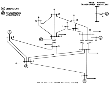
Figure 1: The IEEE 14 Bus Test Case [19].

Figure 2: Hourly Germany load and solar generation data from Aug 2, 2015 to Aug 8, 2015 [18].

Weather data were used in order to design the machine learning models. The Weather Company’s Cleaned Observations application programming interface (API) [20] provides cleaned, interpolated, historical observations of a wide variety of weather variables. Version two of the API was used to retrieve hourly historical observations of surface temperature, diffuse horizontal radiation, direct normal irradiance, and downward solar radiation at 52.52°N, 13.61°E (Berlin) from Jan 1, 2014, to Aug 8, 2015. A more rigorous choice would have been to use a combination of points appropriately distributed across Germany. A simple approach was however favoured as it did not impact the objectives of the proposed experiments.

IV-B Experimental Setup for the Data Fusion Model

Based on the load and solar generation profiles shown in Fig. 2, a realistic simulation of the 14-bus system is provided as follows. The active injection at each network bus provided by the standard model in [19] is taken to represent the peak load over the validation week (Aug 2 to Aug 8, 2015). The hourly profile is then modulated according to the load profile. It is further assumed that the solar generation is uniformly spread across the load buses 3 to 6 and 9 to 14, such to obtain the demand and generation components of the active load.

The data fusion model was then built based on the assumptions that data were generated from three different systems, producing the factor graph shown in Figure 3. Details of the factor nodes are outlined in the following.

Figure 3: Factor graph representation of the power systems data fusion model used in the experiments. Squares denote factors, circles are variable nodes.

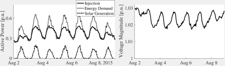
Figure 4: Simulated data sources: (a) Active power injection, energy demand, solar generation and voltage magnitude at bus 4; (b) Forecasts of energy demand and solar generation at bus 4, with the $95\%$ confidence interval.

IV-B1 State Estimation Factor Node

A set of data, $y_{1}$, is generated based on a power flow simulation of the 14-bus system. It is assumed that measurements are available for all active/reactive power injections and voltage magnitudes. Measurement data were generated by simulating the 14-bus power flow using Matpower [21] and the available load profiles. White Gaussian noise with standard deviation of $0.01$ p.u. for the power measurements and of $0.5e^{-3}$ p.u. for the voltage magnitudes was introduced. Figure 4 shows an example of active power and voltage magnitude measurements generated at bus 4. The state variables, $x_{1}$, were defined as the set of bus voltages and measurement model, $y_{1}=f_{1}(x_{1})+\varepsilon_{1}$, was based on the usual AC power flow equations [5].

IV-B2 Smart Meters Factor Node

Smart meter data, $y_{2}$, were assumed to provide total energy demand and solar generation at the 10 load buses of the system, buses 3 to 6 and 9 to 14. White Gaussian noise with standard deviation of $0.02$ p.u. was introduced. Figure 4 shows an example of the energy demand and generation data simulated at bus 4. The hidden state variable, $x_{2}$, was defined as representing the amount of energy demand and solar generation at each bus, so that the relation in (1) is an identify matrix, namely $y_{2}=x_{2}+\varepsilon_{2}$.

IV-B3 Machine Learning Factor Node

Forecasting models providing data, $y_{3}$, of energy demand and solar generation at the 10 load buses specified in the state variable $x_{2}$ were also considered, so that the same model as for the smart meter factor node, $y_{3}=x_{2}+\varepsilon_{3}$, was utilized.

The forecasts were computed using generalized additive models (GAMs) based on penalized iteratively re-weighted least squares method [22, 23]. Extensive research has gone into studying the covariates that are important to model electricity (see [13, 24, 22] and references within). The energy demand model considered in this study is given by:

$$D=s_{1}(\text{hour},\text{daytype})+s_{2}(T_{m})+s_{3}(T_{max})+\zeta$$ (19)

where $D$ is the energy demand at a given time instant, daytype is a categorical variable representing each day of a week, hour is the numerical variable representing the hour in a day, $T_{m}$ is the mean temperature for the day and $T_{max}$ is the maximum temperature of the day. The basis functions $s_{i}(u)$ are smooth splines based on cubic B-splines. The solar generation forecast model was considered to be a linear model with normal and diffuse irradiance data as covariates.

The models were trained on the period from January 1, 2014 to August 1, 2015, and a sample output for bus 4 is shown in Fig. 4. A mean absolute percentage error for the demand forecasts of about $4.3\%$ was observed on the validation week between August 2 and August 8, 2015. For the solar generation forecasts, a $10.4\%$ error was observed (normalized on the daily peak of generation to avoid numerical issues when generation is near the zero). Improved demand models could be designed by considering a more extensive set of features. Similarly, better solar generation forecasts can be obtained, for example by exploiting non-linead physics-based models [3]. However the focus of the paper is not on energy forecasting and such alternatives were not pursued.

IV-B4 Joint Factor Node

A joint factor relating the state variables $x_{1}$ and $x_{2}$ was designed as:

$$0=f_{41}(x_{1})-F_{42}x_{2}+\varepsilon_{4},\\$$ (20)

where $f_{41}(x_{1})$ represents the active injection equations of the AC power flow model, and $F_{42}$ is a matrix where each row has a $+1$ and a $-1$ in correspondence, respectively, of the demand and generation entries in the state variable $x_{2}$ at the specific network bus. The Gaussian random error $\varepsilon_{4}\sim\mathbb{N}(0,R_{4})$ is chosen such thah $R_{4}$ is a diagonal matrix with very small diagonal entries of $1e-10$.

IV-C Experimental results

Since the factor graph contains no loops, as noted in section III-B, the proposed inference algorithm is equivalent to solving the global problem (2)-(3) with the Gauss-Newton method. However, instead of computing one matrix inversion of dimension $n_{1}+n_{2}$, four matrix inversions of dimension $n_{1}$ and $n_{2}$ are performed at every iteration, based on (15) and (17). As the number and dimensionality of the nodes increases, significant computational gain can be obtained.

In a first experiment, the proposed inference algorithm was run on the simulated data over the validation week. Convergence was achieved in less then 10 steps for all 168 hourly samples. As expected, fusion of the three data sources allows reduction of uncertainty in estimating the true quantities with respect to using the information from the individual sources alone. As shown in Figure 5, the estimation of energy demand and solar generation at the bus 4, which is only metered directly from the smart meter data, also benefits from fusion with the state estimation node, and shows lower error than when using the raw data only. Although not shown here, the improvement is consistent across all the network buses.

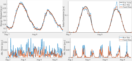
Figure 5: Comparison between fused data and raw data of energy demand and solar genertaion at bus 4.

In a second experiment, loss of observability on the last 2 days of the validation period is considered in the state estimation node. In particular, voltages, active/reactive power and smart meter data are assumed unavailable from network buses 3, 4, 9 and 10 (bottom right of network diagram in Fig. 1). It can be shown that in this case the state estimation node has a singularity, but the belief propagation algorithm does not experience invertibility issues since, through (13) and (15), implicitly applies a regularization based on information available from the energy forecasts node. Fused information is still obtained, although with higher uncertainty than when all data are available, as shown in Fig. 6 for bus 4.

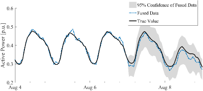
Figure 6: Estimation of the active power injection at bus 4, with loss of observability in the state estimation node on August 7. The confidence interval before Aug 7 is not visible as much smaller than after loss of observability.

A final experiment shows how inconsistencies in a data source can be detected through data fusion. It is assumed that new solar installations cause an increase of $50\%$ capacity at bus 4 in the last 2 days of the validation period, and that this is not reflected in the smart meter data (actually, a typical real-world scenario). Figure 7 shows how the fused estimate of solar generation at bus 4 is in larger than the raw data and closer to the true value by an amount comparable to the confidence interval. The possible inconsistency can be formally detected using statistical testing. Obviously such information comes from the grid data which are affected by the increased solar generation at the bus.

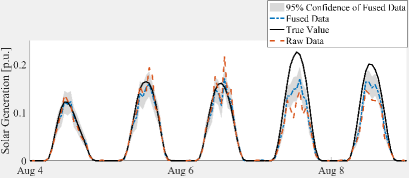
Figure 7: Fused data and true value of solar generation at bus 4, when new solar capacity becomes available on August 7 but is not reflected in raw data.

V Conclusion

In this study, a novel computational framework for power systems data fusion was proposed. Based on probabilistic graphical models, heterogeneous data sources and related measurement models (physical laws or data-driven machine learning models) can be combined such that a consistent and unified view of the system is obtained. An efficient and naturally distributed inference algorithm based on Gaussian belief propagation is also derived.

In a set of numerical examples it was demonstrated how the traditional notion of state can be extended to provide visibility into the amount of solar generation at the buses of a network model. The fused information reduces the effect of noise in the various data sources and occurrences of missing or erroneous data are easily overcome and diagnosed.

While fully known measurement functions were assumed, future work will investigate scenarios where they are partly unknown and need to be learned from the data. Further possibility for extensions of the state variable to include, for example, effects of temperature variation or of demand response programs on the active injections will also be investigated. Since the data consistency is one the key benefits of data fusion, extensions of traditional bad data analysis to the proposed framework is also of interest for future studies.

References

- [1] N. Yu, S. Shah, R. Johnson, R. Sherick, M. Hong, M. Ieee, and K. Loparo, “Big Data Analytics in Power Distribution Systems,” in Proceedings of the Innovative Smart Grid Technologies Conference, Washington, DC, USA, 2015.
- [2] S. E. Collier, “The emerging enernet: Convergence of the smart grid with the internet of things,” IEEE Industry Applications Magazine, vol. 23, no. 2, 2017.
- [3] V. P. A. Lonij, J.-B. Fiot, B. Chen, F. Fusco, P. Pompey, Y. Gkoufas, M. Sinn, D. Tougas, M. Coombs, and A. Stamp, “A scalable demand and renewable energy forecasting system for distribution grids,” IEEE Power and Energy Society General Meeting (PESGM), 2016.
- [4] F. Fusco, U. Fischer, V. Lonij, P. Pompey, J.-B. Fiot, B. Chen, Y. Gkoufas, and M. Sinn, “Data management system for energy analytics and its application to forecasting,” Proceedings of the Workshops of the EDBT/ICDT Joint Conference 2016, 2016.
- [5] A. Abur and A. G. Exposito, Power System State Estimation: Theory and Implementation. CRC Press, 2004.
- [6] A. Monticelli, “Electric power system state estimation,” Proceedings of the IEEE, vol. 88, no. 2, pp. 262–282, feb 2000.
- [7] E. Manitsas, R. Singh, B. Pal, and G. Strbac, “Modelling of Pseudo-Measurements for Distribution System State Estimation,” in CIRED Seminar 2008: SmartGrids for Distribution, 2008.
- [8] J. Wu, Y. He, and N. Jenkins, “A Robust State Estimator for Medium Voltage Distribution Networks,” IEEE Trans. on Power Systems, 2012.
- [9] Y. Hu, A. Kuh, A. Kavcic, and T. Yang, “A Belief Propagation Based Power Distribution System State Estimator,” IEEE Computational Intelligence Magazine, no. AUGUST, pp. 36–46, 2011.
- [10] M. Cosovic and D. Vukobratovic, “State estimation in electric power systems using belief propagation: An extended dc model,” IEEE International workshop on Signal Processing advances in Wireless Communications (SPAWC), 2016.
- [11] ——, “Distributed gauss-newton method for ac state estimation: A belief propagation approach,” IEEE International Conference on Smart Grid Communications, 2016.
- [12] D. S. Callaway and I. A. Hiskens, “Achieving controllability of electrical loads,” Proceedings of the IEEE, 2011.
- [13] R. Weron, Modeling and forecasting electricity loads and prices: A statistical approach. John Wiley & Sons, 2007, vol. 403.
- [14] B. J. Frey and N. Jojic, “A comparison of algorithms for inference and learning in probabilistic graphical models,” IEEE Transactions on Pattern Analysis and Machine Intelligence, vol. 27, no. 9, 2005.
- [15] H.-A. Loelinger, “An introduction to factor graphs,” IEEE Signal Processing Magazine, 2004.
- [16] H.-A. Loelinger, J. Dauwels, J. Hu, S. Korl, L. Ping, and F. R. Kschischang, “The factor graph approach to model-based signal processing,” Proceedings of the IEEE, 2007.
- [17] D. Barber, Bayesian Reasoning and Machine Learning. Cambridge University Press, 2012.
- [18] Open Power System Data, “Data package time series,” 2017. [Online]. Available: http://data.open-power-system-data.org/time_series/2017-03-06/
- [19] University of Washington, “Power Systems Test Case Archive,” 2013. [Online]. Available: http://www.ee.washington.edu/research/pstca/
- [20] The Weather Company, “Cleaned observations api,” 2017. [Online]. Available: http://cleanedobservations.wsi.com/documents/WSI%20Cleaned%20Observations%20API%20Documentation.pdf
- [21] R. D. Zimmerman, C. E. Murillo-Sánchez, and R. J. Thomas, “Matpower: Steady-state operations, planning and analysis tools for power systems research and education,” Power Systems, IEEE Transactions on, vol. 26, no. 1, pp. 12–19, 2011.
- [22] A. Ba, M. Sinn, Y. Goude, and P. Pompey, “Adaptive Learning of Smoothing Functions : Application to Electricity Load Forecasting,” in Proceedings of the Neural Information Processing Systems (NIPS) Conference, Lake Tahoe, Nevada, USA, 2012.
- [23] S. N. Wood, Y. Goude, and S. Shaw, “Generalized additive models for large data sets,” Journal of the Royal Statistical Society: Series C (Applied Statistics), vol. 64, no. 1, pp. 139–155, 2015.
- [24] A. Pierrot and Y. Goude, “ Short-Term Electricity Load Forecasting With Generalized Additive Models ,” in 16th Intelligent System Applications to Power Systems Conference (ISAP), 2011.