Conjoined constraints on modified gravity from the expansion history and cosmic growth

Abstract

In this paper we present conjoined constraints on several cosmological models from the expansion history $H(z)$ and cosmic growth $f\sigma_{8}(z)$. The models we study include the CPL $w_{0}w_{a}$ parametrization, the Holographic Dark Energy (HDE) model, the Time varying vacuum ($\Lambda_{t}$CDM) model, the Dvali, Gabadadze and Porrati (DGP) and Finsler-Randers (FRDE) models, a power law $f(T)$ model and finally the Hu-Sawicki $f(R)$ model. In all cases we perform a simultaneous fit to the SnIa, CMB, BAO, $H(z)$ and growth data, while also following the conjoined visualization of $H(z)$ and $f\sigma_{8}(z)$ as in Linder (2017). Furthermore, we introduce the Figure of Merit (FoM) in the $H(z)-f\sigma_{8}(z)$ parameter space as a way to constrain models that jointly fit both probes well. We use both the latest $H(z)$ and $f\sigma_{8}(z)$ data, but also LSST-like mocks with $1\%$ measurements and we find that the conjoined method of constraining the expansion history and cosmic growth simultaneously is able not only to place stringent constraints on these parameters but also to provide an easy visual way to discriminate cosmological models. Finally, we confirm the existence of a tension between the growth rate and Planck CMB data and we find that the FoM in the conjoined parameter space of $H(z)-f\sigma_{8}(z)$ can be used to discriminate between the $\Lambda$CDM model and certain classes of modified gravity models, namely the DGP and $f(T)$.

I Introduction

The portrait of the cosmos, as it is revealed by the analysis of various independent cosmological observations (see Ref.Ade et al. (2016) and references therein), is tightly tied with a spatially flat universe in which the cosmic fluid contains $\sim 30\%$ of matter (baryonic and dark) and the rest is the so called dark energy (DE). Although there is mounting observational evidence that DE is responsible for the accelerated expansion of the universe, the underlying mechanism behind such a phenomenon is yet unknown.

Despite the lack of our knowledge regarding the nature of the DE, in the literature there is a large class of cosmological models which mathematically treats the accelerated expansion of the Universe. In general these cosmological scenarios are split into two large groups. The first category of DE models adhere to General Relativity (GR) and propose the existence of new fields in nature (for review see Copeland et al. (2006); Caldwell and Kamionkowski (2009) and references therein). The second group of cosmological models is mainly based on modified gravity for which the present accelerating era appears as a geometric effect due to the fact that gravity becomes weak at cosmological scales Copeland et al. (2006); Clifton et al. (2012). It is interesting to mention that in the context of modified gravity models the effective equation-of-state (EoS) parameter can enter in the phantom regime, namely $w<-1$.

At the perturbation level, the growth of matter fluctuation provides a useful tool to investigate the matter distribution in the Universe Okumura et al. (2016), and, more importantly, it can be measured from observations. Indeed the growth rate data are mainly based on galaxy surveys, like SDSS, BOSS, WiggleZ etc (see our Table 2 and references therein). The growth rate data have been used extensively in the literature in order to put constraints on the growth index $\gamma$. The measurement of the growth index provides an efficient way to discriminate between modified gravity models and DE models which are developed in the context of GR. Indeed, one can find a large family of studies in which the predicted growth index is given analytically for various DE models, including scalar field DE Silveira and Waga (1994); Wang and Steinhardt (1998); Linder and Jenkins (2003); Linder (2004); Nesseris and Perivolaropoulos (2008), DGP Lue et al. (2004); Linder (2004); Gong (2008), $f(R)$ Gannouji et al. (2009); Tsujikawa et al. (2009); Boubekeur et al. (2014), Finsler-Randers Basilakos and Stavrinos (2013), time varying vacuum models $\Lambda(H)$, Basilakos and Sol (2015)), Clustered DE Mehrabi et al. (2015a), Holographic dark energy Mehrabi et al. (2015b) and $f(T)$ Basilakos (2016).

From the aforementioned discussion it becomes clear that up to now the expansion data and the growth data have been used separately in order to study the cosmic history at the background and perturbations levels respectively. In this article we follow a different path, namely the conjoined method recently proposed by Linder Linder (2017) where it was claimed that in order to distinguish the DE models it is better to use the Hubble parameter $H(z)$ directly with the growth quantity $f\sigma_{8}(z)$ in a conjoined diagram, rather than using each as a function of redshift. In the current article we attempt to investigate such a possibility by computing the $H-f\sigma_{8}$ diagram of the most popular DE models and comparing the corresponding predictions with the observed conjoined diagram provided by the cosmic chronometer $H(z)$ and the growth data. A similar, but not overlapping analysis, of the conjoined constraints was also made by Ref. Moresco and Marulli (2017), where the authors studied extensions of the $\Lambda$CDM model, such as a constant but free equation of state $w$ or the effect of neutrinos. However, we consider a much bigger ensemble of dark energy models, hence our analysis in much more broad in scope.

The layout of the article is as follows: In Sec. II we discuss the linear growth of matter fluctuations in the dark energy regime, while in Sec. III we present the basic properties of various cosmological models, including those of modified gravity. In Sec. IV we discuss the tension between the growth and Planck15 CMB data, while in Sec. V, we test the DE cosmologies by comparing the theoretical predictions of the conjoined $H-{\rm{\it f\sigma_{8}}}$ diagram with observations. Finally, we present our conclusions in Sec. VI.

II Linear growth of matter Perturbations

In this section we present the main ingredients of the linear growth of matter perturbations within the context of different types of dark energy. Since we are in the matter dominated epoch we can neglect the radiation component from the cosmic expansion. Let us start the current analysis with the basic differential equation at subhorizon scales Lue et al. (2004); Linder (2004); Gannouji et al. (2009); Stabenau and Jain (2006); Uzan (2007); Tsujikawa et al. (2008)

$$\ddot{\delta}_{m}+2{\tilde{\nu}}H\dot{\delta}_{m}-4\pi G\mu\rho_{m}\delta_{m}=0\;.$$ (1)

As is well known, a general solution of the aforementioned equation is written as $\delta_{m}\propto D(t)$. Notice, that $D(t)$ is the growth factor usually scaled to unity at the present time. In order to address the issue of how the quantities ${\tilde{\nu}}$ and $\mu\equiv G_{\rm eff}/G_{N}$ affect the matter fluctuations, one has to deal in general with the following three distinct scenarios:

1. The situation in which the dark energy models (quintessence and the like) adhere to GR, hence $({\tilde{\nu}},\mu)=(1,1)$.

2. The case where $({\tilde{\nu}},\mu)\neq(1,1)$ which implies that there are interactions in the dark sector and, finally.

3. The case of either modified gravity models or inhomogeneous dark energy models (inside GR), hence ${\tilde{\nu}}=1$ and $\mu\neq 1$.

Now we are ready to introduce the growth rate of clustering (first proposed by Ref. Peebles (1994)) as follows

$$f(a)=\frac{d\ln\delta_{m}}{d\ln a}\simeq\Omega^{\gamma}_{m}(a)$$ (2)

with

$$\Omega_{m}(a)=\frac{\Omega_{m0}a^{-3}}{E^{2}(a)}$$ (3)

where $E(a)=H(a)/H_{0}$ is the normalized Hubble parameter and $\gamma$ is the growth index. By differentiating Eq.(3) it is easy to show

$$\frac{d\Omega_{m}}{da}=-3\frac{\Omega_{m}(a)}{a}\left(1+\frac{2}{3}\frac{d{\rm ln}E}{d{\rm ln}a}\right)\;.$$ (4)

Furthermore, combining Eqs.(2)-(4) the main equation (1 becomes

$$a\frac{df}{da}+\left(2{\tilde{\nu}}+\frac{d{\ln}E}{d{\rm ln}a}\right)f+f^{2}=\frac{3\mu\Omega_{m}}{2},$$ (5)

or

$$a{\rm ln}(\Omega_{m})\frac{d\gamma}{da}+\Omega_{m}^{\gamma}-3\gamma+2{\tilde{\nu}}-\left(\gamma-\frac{1}{2}\right)\frac{d{\ln}E}{d{\rm ln}a}=\frac{3}{2}\mu\Omega_{m}^{1-\gamma}.$$ (6)

It is interesting to mention that Steigerwald et al. Steigerwald et al. (2014) have provided another expression of the above equation, namely

$$\frac{d\omega}{d{\ln}a}(\gamma+\omega\frac{d\gamma}{d\omega})+{\rm e}^{\omega\gamma}+2{\tilde{\nu}}+\frac{d{\ln}E}{d{\rm ln}a}=\frac{3}{2}\mu{\rm e}^{\omega(1-\gamma)},$$ (7)

where $\omega={\rm ln}\Omega_{m}(a)$ which implies that at $z\gg 1$ ($a\to 0$) we get $\Omega_{m}(a)\to 1$ [or $\omega\to 0$]. Based on Eq.(7) Steigerwald et al. Steigerwald et al. (2014) proposed a general mathematical approach in order to derive the asymptotic value of the growth index which is given by (see Eq.(8) in Ref. Steigerwald et al. (2014) and the relevant discussion in Ref. Basilakos and Sol (2015))

$$\gamma_{\infty}=\frac{3(M_{0}+M_{1})-2(H_{1}+N_{1})}{2+2X_{1}+3M_{0}},$$ (8)

where

$$M_{0}=\left.\mu\right|_{\omega=0}\,,\ \ M_{1}=\left.\frac{d\mu}{d\omega}\right|_{\omega=0}$$ (9)

and

$$N_{1}=\left.\frac{d{\tilde{\nu}}}{d\omega}\right|_{\omega=0}\,,\ \ H_{1}=-\frac{X_{1}}{2}=\left.\frac{d\left(d{\rm ln}E/d{\rm ln}a\right)}{d\omega}\right|_{\omega=0}\,.$$ (10)

Since the exact functional form of the growth index has yet to be found, here we utilize the well known Taylor expansion around $a(z)=1$ (see Ref. Polarski and Gannouji (2008); Bueno belloso et al. (2011); Di Porto et al. (2012))

$$\gamma(a)=\gamma_{0}+\gamma_{1}(1-a),$$ (11)

in which the asymptotic value boils down to $\gamma_{\infty}\simeq\gamma_{0}+\gamma_{1}$, where we have set $\gamma_{0}=\gamma(1)$. Lastly, writing Eq.(6) at the present time ($a=1$)

$$-\gamma^{\prime}(1){\rm ln}(\Omega_{m0})+\Omega_{m0}^{\gamma(1)}-3\gamma(1)+2{\tilde{\nu}}_{0}-2(\gamma_{0}-\frac{1}{2})\left.\frac{d{\ln}E}{d{\rm ln}a}\right|_{a=1}$$

$$=\frac{3}{2}\mu_{0}\Omega_{m0}^{1-\gamma(1)},\ \ \$$ (12)

and with the aid of Eq.(11) we arrive at

$$\gamma_{1}=\frac{\Omega_{m0}^{\gamma_{0}}-3\gamma_{0}+2{\tilde{\nu}}_{0}-2(\gamma_{0}-\frac{1}{2})\left.\frac{d{\ln}E}{d{\rm ln}a}\right|_{a=1}-\frac{3}{2}\mu_{0}\Omega_{m0}^{1-\gamma_{0}}}{\ln\Omega_{m0}}\;,$$ (13)

where prime denotes a derivative with respect to the scale factor, $\mu_{0}=\mu(1)$ and ${\tilde{\nu}}_{0}={\tilde{\nu}}(1)$.

III Dark Energy Models

In this section we describe the ten distinct cosmological models used in our analysis. Notice that the observational viability of these DE models was recently tested in Basilakos and Nesseris Basilakos and Nesseris (2016) using the JLA supernovae, the BAO data and the CMB shift parameters, but also the $H(z)$ data shown in Table 1. We also used a growth-rate data compilation which we now update to the “Gold-2017” set of Ref. Nesseris et al. (2017), shown for completeness in Table 2. For the details of the analysis of the JLA, BAO, CMB and $H(z)$ data we refer the interested reader to Ref. Basilakos and Nesseris (2016), while for that of the new growth-rate data we refer to Ref. Nesseris et al. (2017). The best-fit parameters and their errors for all of the models used in this analysis were obtained via an MCMC, and the results are shown in Table 3.

Knowing the basic cosmological functions of a given dark energy model and the corresponding model parameters, it is trivial to compute the asymptotic value of the growth index $\gamma_{\infty}$ from Eq. (8). The next step is to solve the system of $\gamma_{\infty}=\gamma_{0}+\gamma_{1}$ and Eq.(13) in order to compute $(\gamma_{0},\gamma_{1})$ from the cosmological parameters. Let us now briefly present the cosmological models explored in the current work. Notice, that in all cases we assume a spatially flat Friedmann-Lemaître-Robertson-Walker (FLRW) geometry.

• $w$CDM model. In this case we consider as constant the equation of state (hereafter EoS) parameter $w=p_{d}/\rho_{d}$, where $p_{d}$ and $\rho_{d}$ are the pressure and density of the dark energy fluid respectively. Since this model is inside GR and does not allow interactions in the dark sector we have $\mu(a)={\tilde{\nu}}(a)=1$. The latter conditions imply that the dimensionless Hubble parameter is written as

  $$E^{2}(a)=\Omega_{m0}a^{-3}+\Omega_{d0}a^{-3(1+w)},$$ (14)

  where the model parameters are $\Omega_{m0}=1-\Omega_{d0}$ and $w$. Using Eq.(14) we find

  $$\frac{d{\ln}E}{d{\rm ln}a}=-\frac{3}{2}-\frac{3}{2}w\left[1-\Omega_{m}(a)\right]$$ (15)

  and

  $$\{M_{0},M_{1},H_{1},X_{1}\}=\{1,0,\frac{3w}{2},-3w\}\;.$$

  Inserting the above coefficients into Eq.(8) we recover the well-known asymptotic value of the growth index (see also Ref. Silveira and Waga (1994); Wang and Steinhardt (1998); Linder and Jenkins (2003); Lue et al. (2004); Linder (2004); Nesseris and Perivolaropoulos (2008); Basilakos and Pouri (2012)), namely

  $$\gamma_{\infty}=\frac{3(w-1)}{6w-5}.$$

  As expected for $w=-1$ the $w$CDM model reduces to a $\Lambda$CDM cosmological model in which $\gamma_{\infty}^{(\Lambda)}=6/11$.

• CPL model ($w_{0}w_{a}$CDM). This phenomenological model was first proposed by Chevalier-Polarski-Linder Chevallier and Polarski (2001); Linder (2003). Specifically, the dark energy EoS parameter is given as a first order Taylor expansion around the present epoch, $w(a)=w_{0}+w_{1}(1-a)$. This model shares the same cosmological properties with $w$CDM which means that $\mu(a)={\tilde{\nu}}(a)=1$. The normalized Hubble parameter is given by

  $$E^{2}(a)=\Omega_{m0}a^{-3}+\Omega_{d0}a^{-3(1+w_{0}+w_{1})}e^{3w_{1}(a-1)}.$$

  where the free parameters of the models are $(\Omega_{m0},w_{0},w_{1})$ with $\Omega_{d0}=1-\Omega_{m0}$. The quantity $d{\rm ln}E/d{\rm ln}a$ is given by Eq.(15) but here the EoS parameter is $w=w(a)$. Within this context, the growth coefficients (see also Ref. Steigerwald et al. (2014)) are written as

  $$\{M_{0},M_{1},H_{1},X_{1}\}=\{1,0,\frac{3(w_{0}+w_{1})}{2},-3(w_{0}+w_{1})\}$$

  and thus

  $$\gamma_{\infty}=\frac{3(w_{0}+w_{1}-1)}{6(w_{0}+w_{1})-5}.$$

• Running $\Lambda$ ($\Lambda_{t}$CDM model). Here we allow $\Lambda$ to vary with redshift. Using the notations of Refs. Shapiro and Sola (2002); Espana-Bonet et al. (2004) the evolution of the vacuum is written as $\Lambda(H)=\Lambda_{0}+3\nu\,(H^{2}-H_{0}^{2})$, where $\Lambda_{0}\equiv\Lambda(H_{0})=3\Omega_{\Lambda 0}H^{2}_{0}$. In this case the normalized Hubble parameter takes the form

  $$E^{2}(a)={\tilde{\Omega}}_{\Lambda 0}+{\tilde{\Omega}_{m0}}a^{-3(1-\nu)}\;,$$ (16)

  with

  $$\frac{d{\ln}E}{d{\rm ln}a}=-\frac{3}{2}(1-\nu){\tilde{\Omega}}_{m}(a)\;,$$ (17)

  where we have set ${\tilde{\Omega}}_{m}(a)=\frac{\tilde{\Omega}_{m0}a^{-3(1-\nu)}}{E^{2}(a)}$, ${\tilde{\Omega}_{m0}}\equiv\frac{\Omega_{m0}}{1-\nu}$ and ${\tilde{\Omega}_{\Lambda 0}}\equiv\frac{1-\Omega_{m0}-\nu}{1-\nu}$. Evidently, the free parameters of the model are $({\tilde{\Omega}_{m0}},\nu)$. The basic quantities ${\tilde{\nu}}$ and $\mu$ (see Ref. Basilakos and Sol (2015)) are given by

  $${\tilde{\nu}}=1+\frac{3}{2}\,\nu$$ (18)

  and

  $$\mu(a)=1-\nu-\frac{4\nu}{{\tilde{\Omega}}_{m}(a)}+3\nu(1-\nu).$$ (19)

  Based on the above we compute the growth coefficients Basilakos and Sol (2015)

  $$\{M_{0},M_{1},H_{1},X_{1}\}=\{1-2\nu-3\nu^{2},-\frac{3(1-\nu)}{2},3(1-\nu)\}$$

  from which we provide

  $$\gamma_{\infty}=\frac{6+3\nu}{11-12\nu}\;.$$

• Holographic dark energy (HDE) model. Using the holographic Ng (2001); Horava and Minic (2000) principle in GR ${\tilde{\nu}}(a)=1$ one can show that

  $$w(a)=-\frac{1}{3}-\frac{2\sqrt{\Omega_{\rm d}(a)}}{3s}$$

  and

  $$\frac{d{\rm ln}\Omega_{d}}{d{\rm ln}a}=-\frac{w(a)}{3}\left[1-\Omega_{d}(a)\right]$$

  and

  $$E^{2}(a)=\frac{\Omega_{m0}a^{-3}}{1-\Omega_{d}(a)}\;,$$

  where $\Omega_{d}(a)=1-\Omega_{m}(a)$. Here the cosmological parameters are $\Omega_{m0}$ and $s$. Note, that the expression of $d{\rm ln}E/d{\rm ln}a$ is given by Eq.(14). We would like to stress that the aforementioned three equations produce a system whose solution provides $w(a)$, $\Omega_{d}(a)$ and $E(a)$.

  The intrinsic features of the HDE are characterized by the quantity $\mu(a)$ as follows Mehrabi et al. (2015b)

  $$\mu(a)=\left\{\begin{array}[]{cc}1&\mbox{homogeneous HDE}\\ 1+\frac{\Omega_{\rm d}(a)}{\Omega_{\rm m}(a)}\Delta_{\rm d}(a)(1+3c_{\rm eff}^{2})&\mbox{clustered HDE}\end{array}\right.$$ (20)

  where $c_{\rm eff}^{2}$ is the effective sound speed of the dark energy and $\Delta_{d}=\frac{1+w(a)}{1-3w(a)}$ Batista and Pace (2013); Mehrabi et al. (2015b). For the homogeneous HDE model (hereafter HHDE) we have (see also Ref. Mehrabi et al. (2015b))

  $$\{M_{0},M_{1},H_{1},X_{1}\}=\{1,0,\frac{3w_{\infty}}{2},-3w_{\infty}\}\;.$$

  where $w_{\infty}\simeq-1/3$, while the asymptotic value of the growth index becomes $\gamma_{\infty}=\frac{4}{7}$. The likelihood analysis of Ref. Basilakos and Nesseris (2016) provides $\Omega_{m0}=0.311\pm 0.003$ and $s=0.654\pm 0.006$ from which we get $(\gamma_{0},\gamma_{1})\simeq(0.558,0.013)$.

  Moreover, for clustered HDE (hereafter CHDE) we find

  $$\{M_{0},M_{1},H_{1},X_{1}\}=\{1,-\frac{(1+3c_{\rm eff}^{2})}{3},\frac{3{\rm w}_{\infty}}{2},-3{\rm w}_{\infty}\}$$

  and hence,

  $$\gamma_{\infty}=\frac{3(1-c_{\rm eff}^{2})}{7}\;.$$

  Notice that we impose $c_{\rm eff}^{2}=0$, which means that the sound horizon is small with respect to the Hubble radius and thus DE perturbations grow in a similar fashion to matter perturbations Garriga and Mukhanov (1999); Armendariz-Picon et al. (1999).

• $f(T)$ gravity model ($f_{T}$CDM model). Among the large body of $f(T)$ gravity models here we focus on the power-law scenario first introduced by Bengochea and Ferraro Bengochea and Ferraro (2009), with $f(T)=\alpha(-T)^{b}$, where $\alpha=(6H_{0}^{2})^{1-b}\frac{\Omega_{F0}}{2b-1}$. In this case the dimensionless Hubble parameter is

  $$E^{2}(a,b)=\Omega_{m0}a^{-3}+\Omega_{d0}E^{2b}(a,b)\;,$$ (21)

  and

  $$\frac{d{\ln}E}{d{\rm ln}a}=-\frac{3}{2}\frac{\Omega_{m}(a)}{[1-bE^{2(b-1)}\Omega_{d0}]}$$ (22)

  where $\Omega_{d0}=1-\Omega_{m0}$. Since $b\ll 1$ Linder (2010) we use the approximation of Nesseris et al. Nesseris et al. (2013) in order to simplify Eqs.(21) and (22), namely

  $$E^{2}(a,b)\simeq E^{2}_{\Lambda}(a)+\Omega_{d0}\ln\left[E^{2}_{\Lambda}(a)\right]b+...\;,$$ (23)

  $$\frac{d{\ln}E}{d{\rm ln}a}\simeq-\frac{3}{2}\Omega_{m}(a)\left[1+\frac{\Omega_{d0}b}{E^{2}_{\Lambda}(a)}+...\right].$$ (24)

  For this geometrical model we have ${\tilde{\nu}}=1$, while the quantity $\mu$ is given by (see Ref. Basilakos (2016) and references therein)

  $$\mu(a)=\frac{1}{1+\frac{b\Omega_{d0}}{(1-2b)E^{2(1-b)}}}$$ (25)

  or

  $$\mu(a)\simeq 1-\frac{\Omega_{d0}}{E^{2}_{\Lambda}(a)}\;b+\cdots.$$ (26)

  Using the above expressions we are ready to compute the growth index coefficients of (9) and (10) [see also Ref. Basilakos (2016)]

  $$\{M_{0},M_{1},H_{1},X_{1}\}=\{1,b,-\frac{3(1-b)}{2},3(1-b)\}$$

  from which we derive

  $$\gamma_{\infty}=\frac{6}{11-6b}\;.$$

  Obviously, for $b=0$ we recover the $\Lambda$CDM value $6/11$.

• $f(R)$ gravity ($f_{R}$CDM model). We would like to finish the presentation of the cosmological models with the $f(R)$ model introduced by Hu and Sawicki. As proposed by Basilakos et al. Basilakos et al. (2013), the Lagrangian of the current $f(R)$ model can be equivalently written as

  $$f(R)=R-\frac{2\Lambda}{1+\left(\frac{b\Lambda}{R}\right)^{n}}$$ (27)

  where $n$ is a parameter of the model (we set it to unity without loss of generality). Following the methodology of Ref. Basilakos et al. (2013) the Hubble parameter is given in terms of a series expansion of the solution of the equations on motion around $b=0$, i.e. $\Lambda$CDM, as

  $$H^{2}(a)=H_{\Lambda}^{2}(a)+\sum_{i=1}^{M}b^{i}\delta H_{i}^{2}(a),$$ (28)

  where $H_{\Lambda}$ is the Hubble parameter of the concordance $\Lambda$CDM model. Notice, that $\delta H_{i}^{2}(a)$ is a set of algebraic quantities that can be determined from the equations of motion, see Ref. Basilakos et al. (2013). Moreover, the latter authors found that if we keep the two first non-zero terms ($M=2$) of the series then the approximated Hubble parameter is in excellent agreement with that provided by the numerical solution. Investigating the growth index in this model is not an easy task, since the modified Newton’s constant is a function of both the scale factor $a$ and the scale $k$, ie $G_{\rm eff}=G_{\rm eff}(a,k)$ Tsujikawa (2007). In particular, we have

  $$\mu(a,k)=\frac{G_{\rm eff}(a,k)}{G_{N}}=\frac{1}{F}\frac{1+4\frac{k^{2}}{a^{2}}F_{,R}/F}{1+3\frac{k^{2}}{a^{2}}F_{,R}/F},$$ (29)

  where $F=f^{\prime}(R)$, $F_{,R}=f^{\prime\prime}(R)$ and we have scaled Eq. (29) so that in the case of $b=0$ ($\Lambda$CDM) we recover $\frac{G_{\rm eff}(a,k)}{G_{N}}=1$ as we should. Here we follow Ref. Basilakos et al. (2013) and set $k=0.1h{\rm Mpc}^{-1}\simeq 300H_{0}$, while $\tilde{\nu}(a)=1$.

  Finally, in Ref. Gannouji et al. (2009) one can see that the current $f(R)$ model predicts rather low and rather high values for the growth index parameters, $(\gamma_{0},\gamma_{1})\simeq(0.4,-0.2)$. Due to the $k$-dependence of the effective Newton’s constant in order to obtain the exact values of $(\gamma_{0},\gamma_{1})$ we first need to solve Eq. (5) numerically in order to compute $\gamma_{0}\simeq\frac{\ln(f(1))}{\ln(\Omega_{m0})}$, where $f(1)$ is the growth rate at $a=1$, and then one can utilize Eq. (13) to estimate $\gamma_{1}$.

• Dvali, Gabadadze and Porrati (DGP) gravity model. In the framework of modified gravity models we first introduce that of Dvali, Gabadadze and Porrati Dvali et al. (2000). It is well known that the normalized Hubble parameter takes the form

  $$E(a)=\sqrt{\Omega_{m0}a^{-3}+\Omega_{rc}}+\sqrt{\Omega_{rc}},$$ (30)

  and thus $\Omega_{rc}=(1-\Omega_{m0})^{2}/4$.

  $$\frac{d{\rm ln}E}{d{\rm ln}a}=-\frac{3\Omega_{m}(a)}{1+\Omega_{m}(a)}.$$ (31)

  Here the quantity $\mu(a)=G_{\rm eff}/G_{N}$ takes the form

  $$\mu(a)=\frac{2+4\Omega^{2}_{m}(a)}{3+3\Omega^{2}_{m}(a)}$$

  and ${\tilde{\nu}}(a)=1$. Combining the above equations with Eqs.(9), (10) and (8) we obtain

  $$\{M_{0},M_{1},H_{1},X_{1}\}=\{1,\frac{1}{3},-\frac{3}{4},\frac{3}{2}\}$$

  and $\gamma_{\infty}=\frac{11}{16}$ (see also Refs. Linder (2004); Gong (2008)). Similar to the $\Lambda$CDM model, the DGP gravity model contains one free parameter, namely $\Omega$.

• Finsler-Randers dark energy model (FRDE). The Finsler-Randers version of Finsler geometry has been used in order to build the FRDE model (see Ref. Stavrinos et al. (2008) and references therein). Interestingly, it has been shown that the cosmic expansion of this model coincides with that of DGP gravity Basilakos and Stavrinos (2013). Therefore, Eqs.(30) and (31) are also valid here and thus we use $\Omega_{m}=0.392\pm 0.008$. Although the two dark energy models (FRDE and DGP) are identical at the background level, they deviate at the perturbation level because for the FRDE model we are dealing with $\mu(a)={\tilde{\nu}}(a)=1$ Stavrinos et al. (2008). In this case it has been found that Basilakos and Nesseris (2016) that

  $$\{M_{0},M_{1},H_{1},X_{1}\}=\{1,0,-\frac{3}{4},\frac{3}{2}\}$$

  which implies $\gamma_{\infty}=\frac{9}{16}$.

IV Tension with Planck and previous analyses

At this point, we should stress that by performing the joint analysis of all the data, including the updated growth compilation “Gold-2017” of Ref. Nesseris et al. (2017), we confirm the existence of a tension between the growth rate and the Planck15 data which have been already observed, and also for other low redshift probes, and those discussed in the literature (see Refs. Joudaki et al. (2017); Nesseris et al. (2017); Basilakos (2015)).

This tension was not so obvious in the previous analysis of Basilakos and Nesseris Basilakos and Nesseris (2016) for two reasons: First, the analysis was done in two steps by initially fitting the background to the SnIa, CMB, BAO and $H(z)$ data and then fixing these best-fit parameters $(\Omega_{m},\Omega_{b}h^{2},\cdots)$ before fitting the growth rate data. Second, not only were the growth rate data used were an older compilation with much bigger errors but the corrections required due to the Alcock-Paczynski effect, due to the different fiducial cosmologies assumed in the derivations of the data, were not implemented at the time, unlike in the current analysis or that of Ref. Nesseris et al. (2017). These corrections contribute only up to a few percent, but could in principle bias the results and are thus necessary.

In order to understand why this tension but also the difference in the best-fit values of $(\gamma_{0},\gamma_{1})$ from Ref. Basilakos and Nesseris (2016) occurs, we show in Fig. 1 the best-fit $\gamma_{0}$ for the $\Lambda$CDM model as a function of $\Omega_{m}$ for various values of the $\sigma_{8}$ parameter. As can be seen, for higher values of $\Omega_{m}$ the new $f\sigma_{8}$ data push the best-fit $\gamma_{0}$ to higher values as well or in other words, they are positively correlated. This means that when the Planck cosmology of $\Omega_{m}=0.315$ is used (shown in Fig. 1 with a vertical dashed line), then the best-fit growth index is in the range of $\gamma_{0}\sim 0.73$ in contrast to lower values of $\Omega_{m}$ that prefer a value for the $\gamma_{0}$ parameter closer to $6/11\simeq 0.545$.

Furthermore, with the small arrow we show the Planck $\Lambda$CDM values of $(\gamma_{0},\Omega_{m})=(6/11,0.315)$, which is quite far from our best-fit of $\gamma_{0}=0.725$. Also, it is important to note that the effect of the parameter $\sigma_{8}$ is quite strong, as it can strongly affect the value of the growth index. For example, as shown in Fig. 1, by changing $\sigma$ between $\sigma_{8}\in\left[0.75,0.85\right]$ then the growth index changes by roughly $30\%$. This is also part of the reason for the disagreement with Ref. Basilakos and Nesseris (2016), as the best-fit values of $\sigma_{8}$ in that case were quite lower than in this analysis.

Finally, this tension could be attributed to systematics in the low redshift probes Joudaki et al. (2017), new physics in the form of modifications of gravity and $G_{eff}$ in particular Nesseris et al. (2017), or even in the form of a suppression of power at small scales Kunz et al. (2015).

Figure 1: The best-fit $\gamma_{0}$ for the $\Lambda$CDM model as a function of $\Omega_{m}$ for various values of the $\sigma_{8}$ parameter. As can be seen, the $f\sigma_{8}$ data push the best-fit $\gamma_{0}$ to higher values for higher $\Omega_{m}$. This means that when a Planck cosmology of $\Omega_{m}=0.315$ is used (shown with a vertical dashed line), then the best-fit is in the region of $\gamma_{0}\sim 0.73$ in contrast to lower values of $\Omega_{m}$ that prefer a value for the $\gamma_{0}$ parameter closer to 6/11.

Table 1: The $H(z)$ data used in the current analysis (in units of $\textrm{km}~{}\textrm{s}^{-1}\textrm{Mpc}^{-1}$). This compilation is based partly in those of Refs. Moresco et al. (2016) and Guo and Zhang (2016).

$z$	$H(z)$	$\sigma_{H}$	Ref.
$0.07$	$69.0$	$19.6$	Zhang et al. (2014)
$0.09$	$69.0$	$12.0$	Stern et al. (2010)
$0.12$	$68.6$	$26.2$	Zhang et al. (2014)
$0.17$	$83.0$	$8.0$	Stern et al. (2010)
$0.179$	$75.0$	$4.0$	Moresco et al. (2012)
$0.199$	$75.0$	$5.0$	Moresco et al. (2012)
$0.2$	$72.9$	$29.6$	Zhang et al. (2014)
$0.27$	$77.0$	$14.0$	Stern et al. (2010)
$0.28$	$88.8$	$36.6$	Zhang et al. (2014)
$0.35$	$82.7$	$8.4$	Chuang and Wang (2013)
$0.352$	$83.0$	$14.0$	Moresco et al. (2012)
$0.3802$	$83.0$	$13.5$	Moresco et al. (2016)
$0.4$	$95.0$	$17.0$	Stern et al. (2010)
$0.4004$	$77.0$	$10.2$	Moresco et al. (2016)
$0.4247$	$87.1$	$11.2$	Moresco et al. (2016)
$0.44$	$82.6$	$7.8$	Blake et al. (2012)
$0.44497$	$92.8$	$12.9$	Moresco et al. (2016)
$0.4783$	$80.9$	$9.0$	Moresco et al. (2016)
$0.48$	$97.0$	$62.0$	Stern et al. (2010)
$0.57$	$96.8$	$3.4$	Anderson et al. (2014)
$0.593$	$104.0$	$13.0$	Moresco et al. (2012)
$0.60$	$87.9$	$6.1$	Blake et al. (2012)
$0.68$	$92.0$	$8.0$	Moresco et al. (2012)
$0.73$	$97.3$	$7.0$	Blake et al. (2012)
$0.781$	$105.0$	$12.0$	Moresco et al. (2012)
$0.875$	$125.0$	$17.0$	Moresco et al. (2012)
$0.88$	$90.0$	$40.0$	Stern et al. (2010)
$0.9$	$117.0$	$23.0$	Stern et al. (2010)
$1.037$	$154.0$	$20.0$	Moresco et al. (2012)
$1.3$	$168.0$	$17.0$	Stern et al. (2010)
$1.363$	$160.0$	$33.6$	Moresco (2015)
$1.43$	$177.0$	$18.0$	Stern et al. (2010)
$1.53$	$140.0$	$14.0$	Stern et al. (2010)
$1.75$	$202.0$	$40.0$	Stern et al. (2010)
$1.965$	$186.5$	$50.4$	Moresco (2015)
$2.34$	$222.0$	$7.0$	Delubac et al. (2015)

Table 2: A compilation of robust and independent $f\sigma_{8}(z)$ measurements from different surveys, compiled in Ref. Nesseris et al. (2017). In the columns we show in ascending order with respect to redshift, the name and year of the survey that made the measurement, the redshift and value of $f\sigma_{8}(z)$ and the corresponding reference and fiducial cosmology. These datapoints are used in our analysis in the next sections.

Index	Dataset	$z$	$f\sigma_{8}(z)$	Refs.	Year	Notes
1	6dFGS+SnIa	$0.02$	$0.428\pm 0.0465$	Huterer et al. (2016)	2016	$(\Omega_{m},h,\sigma_{8})=(0.3,0.683,0.8)$
2	SnIa+IRAS	0.02	$0.398\pm 0.065$	Turnbull et al. (2012),Hudson and Turnbull (2013)	2011	$(\Omega_{m},\Omega_{K})=(0.3,0)$
3	2MASS	0.02	$0.314\pm 0.048$	Davis et al. (2011),Hudson and Turnbull (2013)	2010	$(\Omega_{m},\Omega_{K})=(0.266,0)$
4	SDSS-veloc	$0.10$	$0.370\pm 0.130$	Feix et al. (2015)	2015	$(\Omega_{m},\Omega_{K})=(0.3,0)$
5	SDSS-MGS	$0.15$	$0.490\pm 0.145$	Howlett et al. (2015)	2014	$(\Omega_{m},h,\sigma_{8})=(0.31,0.67,0.83)$
6	2dFGRS	$0.17$	$0.510\pm 0.060$	Song and Percival (2009)	2009	$(\Omega_{m},\Omega_{K})=(0.3,0)$
7	GAMA	$0.18$	$0.360\pm 0.090$	Blake et al. (2013)	2013	$(\Omega_{m},\Omega_{K})=(0.27,0)$
8	GAMA	$0.38$	$0.440\pm 0.060$	Blake et al. (2013)	2013
9	SDSS-LRG-200	$0.25$	$0.3512\pm 0.0583$	Samushia et al. (2012)	2011	$(\Omega_{m},\Omega_{K})=(0.25,0)$
10	SDSS-LRG-200	$0.37$	$0.4602\pm 0.0378$	Samushia et al. (2012)	2011
11	BOSS-LOWZ	$0.32$	$0.384\pm 0.095$	Sanchez et al. (2014)	2013	$(\Omega_{m},\Omega_{K})=(0.274,0)$
12	SDSS-CMASS	$0.59$	$0.488\pm 0.060$	Chuang et al. (2016)	2013	$\ \ (\Omega_{m},h,\sigma_{8})=(0.307115,0.6777,0.8288)$
13	WiggleZ	$0.44$	$0.413\pm 0.080$	Blake et al. (2012)	2012	$(\Omega_{m},h)=(0.27,0.71)$
14	WiggleZ	$0.60$	$0.390\pm 0.063$	Blake et al. (2012)	2012
15	WiggleZ	$0.73$	$0.437\pm 0.072$	Blake et al. (2012)	2012
16	Vipers PDR-2	$0.60$	$0.550\pm 0.120$	Pezzotta et al. (2016)	2016	$(\Omega_{m},\Omega_{b})=(0.3,0.045)$
17	Vipers PDR-2	$0.86$	$0.400\pm 0.110$	Pezzotta et al. (2016)	2016
18	FastSound	$1.40$	$0.482\pm 0.116$	Okumura et al. (2016)	2015	$(\Omega_{m},\Omega_{K})=(0.270,0)$

Table 3: The best-fit parameters of the various parameters of the models presented in the previous section.

Model	$\alpha$	$\beta$	$\Omega_{m}$	$\Omega_{b}h^{2}$	$\gamma_{0}$	$\gamma_{1}$	DE params	$h$	$\sigma_{8}$	$\chi^{2}_{min}$
$\Lambda$CDM	$0.141\pm 0.006$	$3.102\pm 0.004$	$0.315\pm 0.003$	$0.0222\pm 0.0001$	$0.725\pm 0.036$	$0.584\pm 0.127$	${}^{w_{0}=-1}_{w_{a}=0}$	$0.673\pm 0.002$	$0.877\pm 0.034$	743.303
$w$CDM	$0.141\pm 0.005$	$3.097\pm 0.005$	$0.318\pm 0.004$	$0.0223\pm 0.0004$	$0.731\pm 0.069$	$0.581\pm 0.058$	${}^{w_{0}=-0.987\pm 0.005}_{w_{a}=0}$	$0.670\pm 0.003$	$0.879\pm 0.033$	743.235
CPL	$0.141\pm 0.004$	$3.100\pm 0.005$	$0.317\pm 0.006$	$0.0222\pm 0.0001$	$0.729\pm 0.036$	$0.576\pm 0.118$	${}^{w_{0}=-0.984\pm 0.008}_{w_{a}=-0.020\pm 0.004}$	$0.671\pm 0.004$	$0.878\pm 0.036$	743.248
DGP	$0.136\pm 0.006$	$3.076\pm 0.017$	$0.390\pm 0.006$	$0.0229\pm 0.0001$	$1.053\pm 0.074$	$0.900\pm 0.092$	$-$	$0.588\pm 0.003$	$1.028\pm 0.046$	844.348
Time Var.	$0.141\pm 0.008$	$3.076\pm 0.008$	$0.319\pm 0.004$	$0.0222\pm 0.0001$	$0.737\pm 0.064$	$0.669\pm 0.123$	${}^{s=(-2.95\pm 13.6)\cdot 10^{-5}}$	$0.671\pm 0.004$	$0.886\pm 0.058$	743.689
Holo	$0.142\pm 0.005$	$3.092\pm 0.008$	$0.314\pm 0.003$	$0.0224\pm 0.0001$	$0.740\pm 0.055$	$0.832\pm 0.055$	$v=0.669\pm 0.008$	$0.669\pm 0.002$	$0.896\pm 0.047$	751.237
$f(R)$	$0.141\pm 0.005$	$3.110\pm 0.013$	$0.317\pm 0.005$	$0.0222\pm 0.0001$	$0.753\pm 0.041$	$0.690\pm 0.062$	$b=0.083\pm 0.005$	$0.671\pm 0.003$	$0.896\pm 0.032$	743.337
$f(T)$	$0.141\pm 0.008$	$3.095\pm 0.027$	$0.317\pm 0.005$	$0.0222\pm 0.0001$	$0.730\pm 0.091$	$0.586\pm 0.067$	$b=0.021\pm 0.013$	$0.671\pm 0.003$	$0.879\pm 0.057$	743.230

V Conjoined Analysis with real and mock data

In this section we implement the conjoined method of Ref. Linder (2017) in order to distinguish the dark energy models, by placing constraints simultaneously on both the expansion history $H(z)$ and the growth of structure $f\sigma_{8}(z)$. Specifically, Ref. Linder (2017) proposed to utilize the expansion history together with the cosmic growth history, namely the joined analysis of $H-f\sigma_{8}$, as a tool for testing the performance of the dark energy models. Obviously, in order to obtain the conjoined histories diagram it is essential to provide a proper collection of the $H-f\sigma_{8}$ data. Concerning the cosmic history we use the latest cosmic chronometer $H(z)$ data (see Table 1 and references therein), while for the growth data we refer the reader to our Table 2.

Table 4: The binned $H(z)-f\sigma_{8}(z)$ growth data based on the original data of Tables 1 and 2.

Bins	$H(z)$	$f\sigma_{8}(z)$
$0\leq z<0.28$	$75.489\pm 2.718$	$0.394\pm 0.023$
$0.28\leq z<0.56$	$83.572\pm 3.501$	$0.443\pm 0.028$
$0.56\leq z<0.84$	$95.540\pm 2.482$	$0.449\pm 0.036$
$0.84\leq z<1.12$	$129.189\pm 10.862$	$0.400\pm 0.110$

Therefore, assuming that the Universe is isotropic, our aim is to correlate the growth as measured in the form of $f\sigma_{8}(z)$ with that of the cosmic expansion via the Hubble measurements $H(z_{\rm h})$ from the cosmic chronometer data, which are measured in the range $0.07\leq z_{\rm h}\leq 2.34$ (see Table 1). More specifically, we implement the following steps:

1. We note that the maximum redshift for the $f\sigma_{8}$ data is $z_{max}=1.4$; hence, we only keep the $H(z)$ data up to that redshift, so that we have a common sample in the same redshift range.

2. We then split both the $f\sigma_{8}$ and the remaining $H(z)$ data in four equal bins and weight the data according to their errors, see Ref. Nesseris and Sapone (2014).

3. For the combined sample we perform a statistical analysis and by using the models and best-fit parameters as mentioned in the previous section, we make the conjoined $H-f\sigma_{8}$ curves as seen in Figs. 2 and 3, along with real and mock data.

4. For the region defined by the $1\sigma$ errors of the best-fit theoretical models in the $H(z)-f\sigma_{8}(z)$ space, we also calculate the Figure of Merit (FoM), which is equal to the inverse of the enclosed area up to the maximum redshift range covered by both models. Then we rank the models according to their constraining power (see Table 5). Note that the higher the FoM, the more constraining the model becomes.

Table 5: The FoM in the $H(z)-{\rm{\it f\sigma_{8}}}(z)$ parameter space in descending order from higher FoM (more constraining) to lower FoM (less constraining).

Model	FoM
$\Lambda$CDM	$0.3767$
$f_{R}$CDM	$0.3733$
$w$CDM	$0.3589$
CPL	$0.3488$
HDE	$0.2509$
$\Lambda_{t}$CDM	$0.2416$
DGP	$0.2288$
FRDE	$0.2288$
$f_{T}$CDM	$0.2223$

Figure 2: The conjoined plots of the cosmic growth $f\sigma_{8}$ vs the cosmic expansion history $H(z)$ based on the real data (blue points) and mock data (yellow points), as described in the text, for the $\Lambda$CDM, $w$CDM, $w_{0}w_{a}$CDM and Holographic models. We also show the 1$\sigma$ error regions in grey.

Figure 3: The conjoined plots of the cosmic growth $f\sigma_{8}$ vs the cosmic expansion history $H(z)$ based on the real data (blue points) and mock data (yellow points), as described in the text, for the Time Varying Vacuum, DGP, $f(R)$ and $f(T)$ models. We also show the 1$\sigma$ error regions in grey.

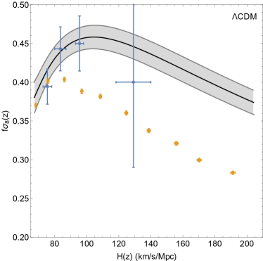
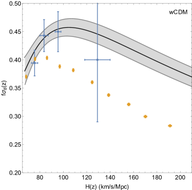
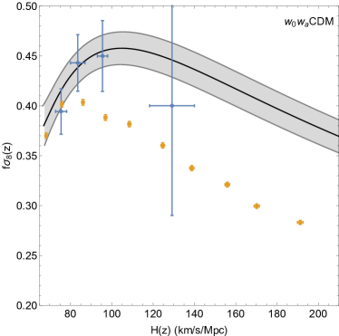
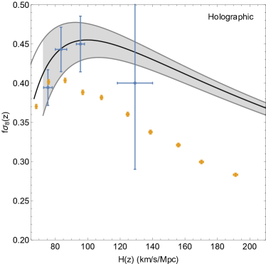
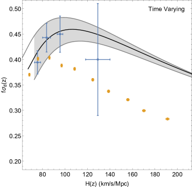
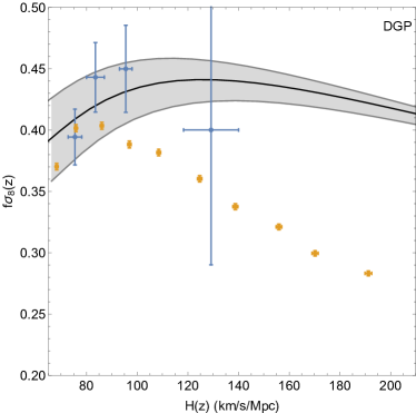
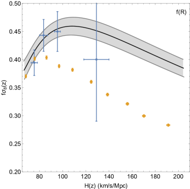
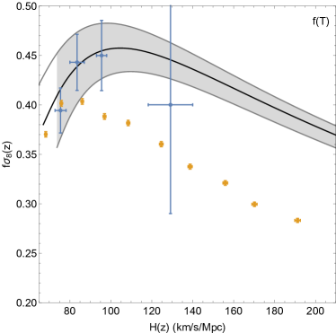
Following the previous steps, we now show in Figs. 2 and 3 the conjoined plots of the cosmic growth $f\sigma_{8}(z)$ vs the cosmic expansion history $H(z)$ based on the real data (blue points) and mock data (yellow points), for the $\Lambda$CDM, $w$CDM, $w_{0}w_{a}$CDM, Holographic, Time Varying Vacuum, DGP, $f(R)$ and $f(T)$ models. We also show the 1$\sigma$ error regions in grey and we use them later on to calculate the $H(z)-{\rm{\it f\sigma_{8}}}(z)$ FoM. In these plots, the real data of Table 2 were split into four equally spaced bins, given in Table 4, while the mock data (yellow points) were based on an LSST-like survey with data in the range $z\in[0,2]$ and a Planck 15 best fit cosmology with $\Omega_{m}$=0.317, $H_{0}=67.2~{}\textrm{km/s/Mpc}$, $w=-1$ and $\sigma_{8}=0.687$. Finally, the mock data were slit into ten equally spaced equally spaced redshift bins.

As can be seen, there is little difference between the theoretical curves of the various models, which is in agreement with our results in Ref. Basilakos and Nesseris (2016). One exception however, is the DGP model which seems to be in strong tension with the data having a $\delta\chi^{2}\sim 100$ with the rest of the models, again confirming our earlier analysis. However, an LSST-like survey, as seen by the mock data (yellow points in Figs. 2 and 3) will be able to discriminate the models and provide stringent constraints on the cosmic growth and expansion history. Furthermore, a survey like this will be able to shed light on the existing tension with Planck by providing data points with very small errors and by minimizing the systematics that occur by combining data from many surveys.

We also calculate the FoM in the $H(z)-{\rm{\it f\sigma_{8}}}(z)$ parameter space, in order to assess how constraining the joined analysis of these data can be. We have defined the FoM as the inverse of the enclosed area of the 1$\sigma$ error regions in Figs. 2 and 3 up to the common maximum redshift $z_{max}=1.4$. We then rank all the models according to their constraining power, noting that the higher the FoM, the more constraining the model becomes.

The result of this comparison is shown in Table 5, where we notice that the $\Lambda$CDM model seems to be much more constraining, followed up closely by the $f_{R}$CDM and $w$CDM models. As mentioned before, the DGP/Finsler models are at the bottom of the ranking, with almost half the constraining power of the rest of the models. Finally, we note that the $f(T)$ model is also at the bottom of the list, something which allows us to discriminate it from the rest of the models even though the model itself is just a perturbation around $\Lambda$CDM. Therefore, the technique of the conjoined analysis of both the $H(z)$ and ${\rm{\it f\sigma_{8}}}(z)$ can in principle discriminate some modifications of gravity from $\Lambda$CDM.

VI Conclusions

In our present study we implemented the $H-f\sigma_{8}$ conjoined method of Ref. Linder (2017) in order to test the viability of a large family of DE models, including the $\Lambda$CDM, $w$CDM, $w_{0}w_{a}$CDM, Holographic, Time Varying Vacuum, DGP, $f(R)$ and $f(T)$ models. First, we combined the available cosmic chronometer and growth data, given in Tables 1 and 2, respectively, and then we identified a common subsample which extends up to redshift $z_{max}=1.4$ and we binned the corresponding data. With this subsample and using the best-fit parameters of the models, as described in Table 3, we then performed the conjoined analysis of the $H-f\sigma_{8}$ parameters, the results of which can be seen in Figs. 2 and 3.

We found that even though there is little difference between the theoretical curves of most of the models, something which is in agreement with our previous results in Ref. Basilakos and Nesseris (2016), we note that the DGP/Finsler class of models seems to be in somewhat strong tension with the data. Also, by analyzing all the data (CMB, SnIa, BAO, growth and $H(z)$), we also observe a strong tension between the growth data and Planck. As mentioned, this tension pushes the values of the growth index $\gamma_{0}$ and $\sigma_{8}$ to be higher than our previous separate analysis.

Furthermore, using a set of mock data, based on an LSST-like survey with Planck15 cosmological parameters, i.e. the yellow points in Figs. 2 and 3, we determined that in the near future we will be able to discriminate the models and provide even stringent simultaneous constraints on the cosmic growth and expansion history.

Using our analysis, we could also quantify the level of the constraining power of these models by using the FoM on the conjoined parameter space of $H-f\sigma_{8}$. The results of this analysis were shown in Table 5. By ranking the models according to their performance, noting that the higher the FoM, the more constraining the model becomes, we found that the $\Lambda$CDM model seems to be the most constraining, followed up closely by the $f_{R}$CDM and $w$CDM models. Again, in agreement with our previous results, we also found that the DGP/Finsler models are at the bottom of the ranking, with almost half the constraining power of the rest of the models.

Finally, we observed that the $f(T)$ model is also at the bottom of the list, something which hints that the conjoined analysis is capable of discriminating such modified gravity models from $\Lambda$CDM, thus proving to be a useful tool given the plethora of dark energy or modified gravity models that are currently available, but also the wealth of data expected from the upcoming surveys in the next decade or so.

References

- Ade et al. (2016) P. A. R. Ade et al. (Planck), Astron. Astrophys. 594, A13 (2016), eprint 1502.01589.
- Copeland et al. (2006) E. J. Copeland, M. Sami, and S. Tsujikawa, Int. J. Mod. Phys. D15, 1753 (2006), eprint hep-th/0603057.
- Caldwell and Kamionkowski (2009) R. R. Caldwell and M. Kamionkowski, Ann. Rev. Nucl. Part. Sci. 59, 397 (2009), eprint 0903.0866.
- Clifton et al. (2012) T. Clifton, P. G. Ferreira, A. Padilla, and C. Skordis, Phys. Rept. 513, 1 (2012), eprint 1106.2476.
- Okumura et al. (2016) T. Okumura et al., Publ. Astron. Soc. Jap. 68, 24 (2016), eprint 1511.08083.
- Silveira and Waga (1994) V. Silveira and I. Waga, Phys. Rev. D50, 4890 (1994).
- Wang and Steinhardt (1998) L.-M. Wang and P. J. Steinhardt, Astrophys. J. 508, 483 (1998), eprint astro-ph/9804015.
- Linder and Jenkins (2003) E. V. Linder and A. Jenkins, Mon. Not. Roy. Astron. Soc. 346, 573 (2003), eprint astro-ph/0305286.
- Linder (2004) E. V. Linder, Phys. Rev. D70, 023511 (2004), eprint astro-ph/0402503.
- Nesseris and Perivolaropoulos (2008) S. Nesseris and L. Perivolaropoulos, Phys. Rev. D77, 023504 (2008), eprint 0710.1092.
- Lue et al. (2004) A. Lue, R. Scoccimarro, and G. D. Starkman, Phys. Rev. D69, 124015 (2004), eprint astro-ph/0401515.
- Gong (2008) Y. Gong, Phys. Rev. D78, 123010 (2008), eprint 0808.1316.
- Gannouji et al. (2009) R. Gannouji, B. Moraes, and D. Polarski, JCAP 0902, 034 (2009), eprint 0809.3374.
- Tsujikawa et al. (2009) S. Tsujikawa, R. Gannouji, B. Moraes, and D. Polarski, Phys. Rev. D80, 084044 (2009), eprint 0908.2669.
- Boubekeur et al. (2014) L. Boubekeur, E. Giusarma, O. Mena, and H. Ram rez, Phys. Rev. D90, 103512 (2014), eprint 1407.6837.
- Basilakos and Stavrinos (2013) S. Basilakos and P. Stavrinos, Phys. Rev. D87, 043506 (2013), eprint 1301.4327.
- Basilakos and Sol (2015) S. Basilakos and J. Sol , Phys. Rev. D92, 123501 (2015), eprint 1509.06732.
- Mehrabi et al. (2015a) A. Mehrabi, S. Basilakos, and F. Pace, Mon. Not. Roy. Astron. Soc. 452, 2930 (2015a), eprint 1504.01262.
- Mehrabi et al. (2015b) A. Mehrabi, S. Basilakos, M. Malekjani, and Z. Davari, Phys. Rev. D92, 123513 (2015b), eprint 1510.03996.
- Basilakos (2016) S. Basilakos, Phys. Rev. D93, 083007 (2016), eprint 1604.00264.
- Linder (2017) E. V. Linder, Astropart. Phys. 86, 41 (2017), eprint 1610.05321.
- Moresco and Marulli (2017) M. Moresco and F. Marulli (2017), eprint 1705.07903.
- Stabenau and Jain (2006) H. F. Stabenau and B. Jain, Phys. Rev. D74, 084007 (2006), eprint astro-ph/0604038.
- Uzan (2007) J.-P. Uzan, Gen. Rel. Grav. 39, 307 (2007), eprint astro-ph/0605313.
- Tsujikawa et al. (2008) S. Tsujikawa, K. Uddin, and R. Tavakol, Phys. Rev. D77, 043007 (2008), eprint 0712.0082.
- Nesseris (2009) S. Nesseris, Phys. Rev. D79, 044015 (2009), eprint 0811.4292.
- Peebles (1994) P. J. E. Peebles, Principles of physical cosmology (1994).
- Steigerwald et al. (2014) H. Steigerwald, J. Bel, and C. Marinoni, JCAP 1405, 042 (2014), eprint 1403.0898.
- Polarski and Gannouji (2008) D. Polarski and R. Gannouji, Phys. Lett. B660, 439 (2008), eprint 0710.1510.
- Bueno belloso et al. (2011) A. Bueno belloso, J. Garcia-Bellido, and D. Sapone, JCAP 1110, 010 (2011), eprint 1105.4825.
- Di Porto et al. (2012) C. Di Porto, L. Amendola, and E. Branchini, Mon. Not. Roy. Astron. Soc. 419, 985 (2012), eprint 1101.2453.
- Basilakos and Nesseris (2016) S. Basilakos and S. Nesseris, Phys. Rev. D94, 123525 (2016), eprint 1610.00160.
- Nesseris et al. (2017) S. Nesseris, G. Pantazis, and L. Perivolaropoulos (2017), eprint 1703.10538.
- Basilakos and Pouri (2012) S. Basilakos and A. Pouri, Mon. Not. Roy. Astron. Soc. 423, 3761 (2012), eprint 1203.6724.
- Chevallier and Polarski (2001) M. Chevallier and D. Polarski, Int. J. Mod. Phys. D10, 213 (2001), eprint gr-qc/0009008.
- Linder (2003) E. V. Linder, Phys. Rev. Lett. 90, 091301 (2003), eprint astro-ph/0208512.
- Shapiro and Sola (2002) I. L. Shapiro and J. Sola, JHEP 02, 006 (2002), eprint hep-th/0012227.
- Espana-Bonet et al. (2004) C. Espana-Bonet, P. Ruiz-Lapuente, I. L. Shapiro, and J. Sola, JCAP 0402, 006 (2004), eprint hep-ph/0311171.
- Ng (2001) Y. J. Ng, Phys. Rev. Lett. 86, 2946 (2001), [Erratum: Phys. Rev. Lett.88,139902(2002)], eprint gr-qc/0006105.
- Horava and Minic (2000) P. Horava and D. Minic, Phys. Rev. Lett. 85, 1610 (2000), eprint hep-th/0001145.
- Batista and Pace (2013) R. C. Batista and F. Pace, JCAP 1306, 044 (2013), eprint 1303.0414.
- Garriga and Mukhanov (1999) J. Garriga and V. F. Mukhanov, Phys. Lett. B458, 219 (1999), eprint hep-th/9904176.
- Armendariz-Picon et al. (1999) C. Armendariz-Picon, T. Damour, and V. F. Mukhanov, Phys. Lett. B458, 209 (1999), eprint hep-th/9904075.
- Bengochea and Ferraro (2009) G. R. Bengochea and R. Ferraro, Phys. Rev. D79, 124019 (2009), eprint 0812.1205.
- Linder (2010) E. V. Linder, Phys. Rev. D81, 127301 (2010), [Erratum: Phys. Rev.D82,109902(2010)], eprint 1005.3039.
- Nesseris et al. (2013) S. Nesseris, S. Basilakos, E. N. Saridakis, and L. Perivolaropoulos, Phys. Rev. D88, 103010 (2013), eprint 1308.6142.
- Basilakos et al. (2013) S. Basilakos, S. Nesseris, and L. Perivolaropoulos, Phys. Rev. D87, 123529 (2013), eprint 1302.6051.
- Tsujikawa (2007) S. Tsujikawa, Phys. Rev. D76, 023514 (2007), eprint 0705.1032.
- Dvali et al. (2000) G. R. Dvali, G. Gabadadze, and M. Porrati, Phys. Lett. B485, 208 (2000), eprint hep-th/0005016.
- Stavrinos et al. (2008) P. C. Stavrinos, A. P. Kouretsis, and M. Stathakopoulos, Gen. Rel. Grav. 40, 1403 (2008), eprint gr-qc/0612157.
- Joudaki et al. (2017) S. Joudaki et al., Mon. Not. Roy. Astron. Soc. 465, 2033 (2017), eprint 1601.05786.
- Basilakos (2015) S. Basilakos, Mon. Not. Roy. Astron. Soc. 449, 2151 (2015), eprint 1412.2234.
- Kunz et al. (2015) M. Kunz, S. Nesseris, and I. Sawicki, Phys. Rev. D92, 063006 (2015), eprint 1507.01486.
- Moresco et al. (2016) M. Moresco, L. Pozzetti, A. Cimatti, R. Jimenez, C. Maraston, L. Verde, D. Thomas, A. Citro, R. Tojeiro, and D. Wilkinson, JCAP 1605, 014 (2016), eprint 1601.01701.
- Guo and Zhang (2016) R.-Y. Guo and X. Zhang, Eur. Phys. J. C76, 163 (2016), eprint 1512.07703.
- Zhang et al. (2014) C. Zhang, H. Zhang, S. Yuan, T.-J. Zhang, and Y.-C. Sun, Res. Astron. Astrophys. 14, 1221 (2014), eprint 1207.4541.
- Stern et al. (2010) D. Stern, R. Jimenez, L. Verde, M. Kamionkowski, and S. A. Stanford, JCAP 1002, 008 (2010), eprint 0907.3149.
- Moresco et al. (2012) M. Moresco et al., JCAP 1208, 006 (2012), eprint 1201.3609.
- Chuang and Wang (2013) C.-H. Chuang and Y. Wang, Mon. Not. Roy. Astron. Soc. 435, 255 (2013), eprint 1209.0210.
- Blake et al. (2012) C. Blake et al., Mon. Not. Roy. Astron. Soc. 425, 405 (2012), eprint 1204.3674.
- Anderson et al. (2014) L. Anderson et al. (BOSS), Mon. Not. Roy. Astron. Soc. 441, 24 (2014), eprint 1312.4877.
- Moresco (2015) M. Moresco, Mon. Not. Roy. Astron. Soc. 450, L16 (2015), eprint 1503.01116.
- Delubac et al. (2015) T. Delubac et al. (BOSS), Astron. Astrophys. 574, A59 (2015), eprint 1404.1801.
- Huterer et al. (2016) D. Huterer, D. Shafer, D. Scolnic, and F. Schmidt (2016), eprint 1611.09862.
- Turnbull et al. (2012) S. J. Turnbull, M. J. Hudson, H. A. Feldman, M. Hicken, R. P. Kirshner, and R. Watkins, Mon. Not. Roy. Astron. Soc. 420, 447 (2012), eprint 1111.0631.
- Hudson and Turnbull (2013) M. J. Hudson and S. J. Turnbull, Astrophys. J. 751, L30 (2013), eprint 1203.4814.
- Davis et al. (2011) M. Davis, A. Nusser, K. Masters, C. Springob, J. P. Huchra, and G. Lemson, Mon. Not. Roy. Astron. Soc. 413, 2906 (2011), eprint 1011.3114.
- Feix et al. (2015) M. Feix, A. Nusser, and E. Branchini, Phys. Rev. Lett. 115, 011301 (2015), eprint 1503.05945.
- Howlett et al. (2015) C. Howlett, A. Ross, L. Samushia, W. Percival, and M. Manera, Mon. Not. Roy. Astron. Soc. 449, 848 (2015), eprint 1409.3238.
- Song and Percival (2009) Y.-S. Song and W. J. Percival, JCAP 0910, 004 (2009), eprint 0807.0810.
- Blake et al. (2013) C. Blake et al., Mon. Not. Roy. Astron. Soc. 436, 3089 (2013), eprint 1309.5556.
- Samushia et al. (2012) L. Samushia, W. J. Percival, and A. Raccanelli, Mon. Not. Roy. Astron. Soc. 420, 2102 (2012), eprint 1102.1014.
- Sanchez et al. (2014) A. G. Sanchez et al., Mon. Not. Roy. Astron. Soc. 440, 2692 (2014), eprint 1312.4854.
- Chuang et al. (2016) C.-H. Chuang et al., Mon. Not. Roy. Astron. Soc. 461, 3781 (2016), eprint 1312.4889.
- Pezzotta et al. (2016) A. Pezzotta et al. (2016), eprint 1612.05645.
- Nesseris and Sapone (2014) S. Nesseris and D. Sapone, Phys. Rev. D90, 063006 (2014), eprint 1405.4769.