Doppler Synthetic Aperture Radar Interferometry: A Novel SAR Interferometry for Height Mapping using Ultra-Narrowband Waveforms

Abstract

This paper introduces a new and novel radar interferometry based on Doppler synthetic aperture radar (Doppler-SAR) paradigm. Conventional SAR interferometry relies on wideband transmitted waveforms to obtain high range resolution. Topography of a surface is directly related to the range difference between two antennas configured at different positions. Doppler-SAR is a novel imaging modality that uses ultra-narrowband continuous waves (UNCW). It takes advantage of high resolution Doppler information provided by UNCWs to form high resolution SAR images.

We introduced the theory of Doppler-SAR interferometry. We derived interferometric phase model and develop the equations of height mapping. Unlike conventional SAR interferometry, we show that the topography of a scene is related to the difference in Doppler between two antennas configured at different velocities. While the conventional SAR interferometry uses range, Doppler and Doppler due to interferometric phase in height mapping, Doppler-SAR interferometry uses Doppler, Doppler-rate and Doppler-rate due to interferometric phase in height mapping. We demonstrate our theory in numerical simulations.

Doppler-SAR interferometry offers the advantages of long-range, robust, environmentally friendly operations; low-power, low-cost, lightweight systems suitable for low-payload platforms, such as micro-satellites; and passive applications using sources of opportunity transmitting UNCW.

1 Introduction

Synthetic Aperture Radar (SAR) interferometry is a powerful tool in mapping surface topography and monitoring dynamic processes. This tool is now an integral part of wide range of applications in many disciplines including environmental remote sensing, geosciences and climate research, earthquake and volcanic research, mapping of Earth’s topography, ocean surface current monitoring, hazard and disaster monitoring, as well as defense and security related research [1].

Basic principles of SAR interferometry were originally developed in radio astronomy [2, 3]. Interferometric processing techniques and systems were later developed and applied to Earth observation [4, 5, 6, 7, 8].

SAR interferometry exploits phase differences of two or more SAR images to extract more information about a medium than present in a single SAR image [9] [10]. Conventional SAR interferometry relies on wideband transmitted waveforms to obtain high range resolution [10, 1, 11, 12, 13]. The phase difference of two wideband SAR images are related to range difference. There are many different interferometric methods depending on the configuration of imaging parameters in space, time, frequency etc [1]. When two images are acquired from different look-directions, the phase difference is related to the topography of a surface.

In this paper, we develop the basic principles of a new and novel interferometric method based on Doppler-SAR paradigm to determine topography of a surface. Unlike conventional SAR, Doppler-SAR uses ultra-narrowband continuous waves (CW) to form high resolution images [14, 15, 16, 17, 18, 19, 20, 21, 22, 23, 24]. Conventional SAR takes advantage of high range resolution and range-rate due to the movement of SAR antenna for high resolution imaging. Doppler-SAR, on the other hand, takes advantage of high temporal Doppler resolution provided by UNCWs and Doppler-rate for high resolution imaging.

We develop the phase relationship between two Doppler-SAR images and show that the phase difference is related to Doppler difference. We approximate this phase difference as Doppler-rate and derive the equations of height mapping for Doppler-SAR interferometry.

Conventional wideband SAR interferometry for height mapping requires two different look-directions. Doppler-SAR interferometry provides a new degree of freedom in system design by allowing antennas to have the same look-direction, but different velocities to obtain height mapping. Additional advantages of Doppler-SAR interferometry include the following: (i) Small, lightweight, inexpensive, easy-to-design and calibrate hardware, high Signal-to-Noise-Ratio(SNR) and long effective range of operation. All of these make Doppler-SAR interferometry a suitable modality for applications requiring high SNR, long range of operation and low payload platforms such as micro-satellites or small uninhabited aerial vehicles. (ii) Effective use of electromagnetic spectrum and environmentally friendly illumination. (iii) Passive applications. Doppler-SAR may not require dedicated transmitters, since existing Radio Frequency (RF) signals of opportunity often have the ultra-narrowband properties.

To the best of our knowledge, this is the first interferometric method that is developed in Doppler-SAR paradigm. We present the theory for two monostatic Doppler-SAR. However, the method can be easily be extended to bistatic and multi-static configurations and synthetic aperture imaging applications in acoustics.

The rest of the paper is organized as follows: In Section 2, SAR geometry and notation are defined. In Section 3, wideband SAR image formation, layover effect and basic principles of wideband SAR interferometry are described in a perspective relevant to our subsequent development. In Section 4, Doppler-SAR data model, image formation and layover are summarized. Section 5 introduces the basic principles of Doppler-SAR interferometry and compares the results to wideband SAR case. Section 6 presents numerical simulations and Section 7 concludes the paper.

2 Configurations and Notation

We consider two mono-static SAR systems as shown in Fig. 1.

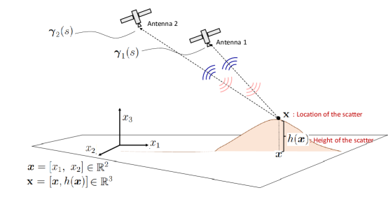
Figure 1: Imaging geometry for an interferometric SAR system with two antennas following trajectories $\bm{\gamma}_{1}(s)$ and $\bm{\gamma}_{2}(s)$. The scatterer is located at $\mathbf{x}\in\mathbb{R}^{3}$ where its height is $h(\bi x)$ and $\bi x=[x_{1},x_{2}]\in\mathbb{R}^{2}$.

Let $\bm{\gamma}_{1}(s)$ and $\bm{\gamma}_{2}(s)$, $s\in[S_{1},\ S_{2}]\subseteq\mathbb{R}$, denote the trajectories of the first and second antennas, respectively.

Unless otherwise stated, bold Roman, bold italic, and Roman lower-case letters will denote elements in $\mathbb{R}^{3}$, $\mathbb{R}^{2}$ and $\mathbb{R}$, respectively, i.e., $\bi x=[x_{1},\ x_{2}]\in\mathbb{R}^{2}$, $x_{3}\in\mathbb{R}$, and $\brmn x=[\bi x,x_{3}]\in\mathbb{R}^{3}$. The Earth’s surface is located at $\brmn x=[\bi x,h(\bi x)]$, where $h:\mathbb{R}^{2}\rightarrow\mathbb{R}$, is the unknown height representing ground topography. Let $V:\mathbb{R}^{3}\rightarrow\mathbb{R}$ denote target reflectivity where we assume that the scattering takes place only on the surface of the Earth. Major notation used throughout the paper is tabulated in Table 1.

Table 1: Notation

Symbol	Description
$\brmn x=[\bi x,h(\bi x)]$, $\brmn x\in\mathbb{R}^{2}$	Location on earth’s surface
$h(\bi x)$	Unknown height of a scatter at $\mathbf{x}$
$V(\brmn x)$	Surface reflectivity
$\bm{\gamma}_{i}(s)$	$i$-th antenna trajectory
$s$	Slow-time
$t$	Fast-time
$R_{i}(\brmn x,s)$	Range of $i$-th antenna
$\omega_{0}$	Center frequency of the transmitted waveforms
$s_{0}^{i}$	Zero-Doppler time for the $i$-th antenna
$\brmn L_{i}(\brmn x,s)$	Look-direction of the $i$-th antenna
$d_{i}^{WB}(t,s)$	Wideband SAR demodulated received signal at $i$-th antenna
$|\mathbf{z}-\bm{\gamma}_{i}(s)|=\mathrm{C.}$	Iso-range surface
$\widehat{(\mathbf{z}-\bm{\gamma}_{i}(s))}\cdot\dot{\bm{\gamma}}_{i}(s)=\mathrm{C}$	Iso-Doppler surface
$\mathcal{K}_{i}^{WB}$	Filtered backprojection (FBP) operator for wideband SAR
$I_{i}^{WB}$	Wideband SAR image
$\Phi^{WB}_{s_{0}}(\mathbf{x})$	Wideband interferometric phase
$\brmn b$	Baseline vector in wideband SAR interferometry
$\brmn L_{1}(\brmn z,s_{0}^{1})\cdot\brmn b=\textmd{C}$	Interferometric phase cone
$\brmn l$	Vector from a known scatterer position to the unknown location of a scatterer
$\mathbf{l}_{1}^{\bot}$	Component of $\brmn l$ perpendicular to $\widehat{(\mathbf{z}_{0}-\bm{\gamma}_{1}(s))}$
$\Phi_{flat}^{WB}(\mathbf{x})$	Flattened wideband SAR interferometric phase
$\phi(t)$	Smooth windowing function
$T_{\phi}$	Duration of $\phi(t)$
$d_{i}^{UNB}(\mu,s)$	Doppler-SAR data
$\brmn L_{i}(\brmn z,s)\cdot\dot{\bm{\gamma}}_{i}(s)=\mathrm{C}$	Iso-Doppler surface
$\brmn L_{i}(\mathbf{z},s)\cdot\ddot{\bm{\gamma}}_{i}(s)-\frac{\dot{\bm{\gamma}}_{i}(s)\cdot\dot{\bm{\gamma}}_{i}^{\perp}(s)}{R_{i}(\mathbf{z},s)}=\mathrm{C}$	Iso-Doppler-rate surface
$\mathcal{K}_{i}^{UNB}$	FBP operator for Doppler-SAR
$I^{UNB}_{i}$	Doppler-SAR image
$\Phi^{UNB}_{s_{d}}(\brmn x)$	Doppler-SAR interferometric phase
$\brmn v$	Baseline velocity
$\Phi_{flat}^{UNB}(\mathbf{x})$	Flattened Doppler-SAR interferometric phase

3 Wideband SAR Interferometry

The basic principles of SAR interferometry are described by many sources [10], [25], [9], [26] [27], [1] and [28]. In this section, we summarize the principles and theory of SAR interferometry in a notation and context relevant to our subsequent presentation of Doppler-SAR interferometry. We begin with the wideband SAR received signal model, derive the interferometric phase model, provide a geometric interpretation of the interferometric phase from which we develop the equations of height mapping.

3.1 Wideband SAR received signal model

We assume that the SAR antennas are transmitting wideband waveforms. Let $r_{i}(t,s)$ denote the received signals, $i=1,2$ where $s$ and $t$ are the slow-time and fast-time variables, respectively. Under the start-stop and Born approximations, the received signals can be modeled as [29, 30, 31]:

$$r_{i}(t,s)=\int{\mathrm{e}}^{-{\mathrm{i}}\omega(t-2R_{i}(\mathbf{x},s)/c)}\tilde{A}_{i}(\brmn x,s,\omega)V(\brmn x){\mathrm{d}}\brmn x{\mathrm{d}}\omega$$ (1)

where

$$R_{i}(\brmn x,s)=|\brmn x-\bm{\gamma}_{i}(s)|$$ (2)

is the range of the $i^{\textmd{th}}$ antenna, $c$ is the speed of light in free-space, $\omega$ is the temporal frequency variable, $V(\brmn x)$ is the scene reflectivity function. $\tilde{A}_{i}$ is a slowly-varying function of $\omega$ that depends on antenna beam patterns, geometrical spreading factors and transmitted waveforms.

Let $\omega=\omega_{0}+\omega^{\prime}$, $\omega^{\prime}\in\Omega$ where $\Omega$ is the bandwith and $\omega_{0}$ is the center frequency of the transmitted waveforms. We demodulate the received signals and write

$$d_{i}^{WB}(t,s) = {\mathrm{e}}^{{\mathrm{i}}\omega_{0}t}r_{i}(t,s),$$ (3)

$$= \int\limits_{-\Omega}^{\Omega}{\mathrm{e}}^{-{\mathrm{i}}\omega^{\prime}(t-2R_{i}(\brmn x,s)/c)}\tilde{A}_{i}(\brmn x,s,\omega^{\prime}){\mathrm{e}}^{{\mathrm{i}}2\frac{\omega_{0}}{c}R_{i}(\brmn x,s)}V(\brmn x){\mathrm{d}}\brmn x{\mathrm{d}}\omega^{\prime}.$$ (4)

Next, we approximate $R_{i}(\brmn x,s)$ in ${\mathrm{e}}^{{\mathrm{i}}\frac{\omega_{0}}{c}R_{i}(\brmn x,s)}$ around $s=s_{0}^{i}$ as follows:

$$R_{i}(\brmn x,s)\approx R_{i}(\brmn x,s_{0}^{i}) + (s-s_{0}^{i})\left.\partial_{s}R_{i}(\brmn x,s)\right|_{s=s_{0}^{i}}$$ (5)

$$+ \frac{(s-s_{0}^{i})^{2}}{2}\left.\ \partial^{2}_{s}R_{i}(\brmn x,s)\right|_{s=s_{0}^{i}},\ i=1,2$$ (6)

where $\partial_{s}$ denotes derivative with respect to $s$ and $s_{0}^{i}$ is the zero-Doppler time for the $i^{\textmd{th}}$ antenna, i.e.,

$$\left.\partial_{s}R_{i}(\brmn x,s)\right|_{s=s_{0}^{i}}=\widehat{(\brmn x-\bm{\gamma}_{i}(s_{0}^{i}))}\cdot\dot{\bm{\gamma}}_{i}(s_{0}^{i})=0.$$ (7)

In (7) $\widehat{\mathbf{x}}$ denotes the unit vector in the direction of $\mathbf{x}$ and $\dot{\bm{\gamma}}_{i}(s)$ denotes the velocity of the $i^{\mathrm{th}}$ antenna.

We define

$$\brmn L_{i}(\brmn x,s)=\widehat{(\brmn x-\bm{\gamma}_{i}(s))}$$ (8)

and refer to $\brmn L_{i}(\brmn x,s)$ as the look-direction of the $i^{\textmd{th}}$ antenna. Note that at the zero-Doppler time, the antenna look-direction is orthogonal to the antenna velocity.

Let

$$A_{i}(\brmn x,s,\omega^{\prime})=\tilde{A}_{i}(\brmn x,s,\omega^{\prime}){\mathrm{e}}^{{\mathrm{i}}2\frac{\omega_{0}}{c}\frac{(s-s_{0}^{i})^{2}}{2}\left[\left.\partial^{2}_{s}R_{i}(s,\brmn x)\right|_{s=s_{0}^{i}}\right]}.$$ (9)

Finally, we write the demodulated received signal as follows:

$$d_{i}^{WB}(t,s) \approx \int\limits_{-\Omega}^{\Omega}{\mathrm{e}}^{-{\mathrm{i}}\omega^{\prime}(t-2R_{i}(\brmn x,s)/c)}A_{i}(\brmn x,s,\omega^{\prime}){\mathrm{e}}^{{\mathrm{i}}2\frac{\omega_{0}}{c}R_{i}(\brmn x,s_{0}^{i})}V(\brmn x){\mathrm{d}}\brmn x{\mathrm{d}}\omega^{\prime}.$$ (10)

3.2 Wideband SAR image formation and layover

Many different algorithms were developed to form wideband SAR images such as range-Doppler [25], seismic migration [32], backprojection [31] and chirp scaling [33] algorithms. All of these algorithms take advantage of high range resolution provided by wideband transmitted waveforms and pulse-to-pulse Doppler information provided by the movement of antennas. The location of a scatterer is identified by intersecting the iso-range and iso-Doppler surfaces and the ground topography as shown in Fig. 2.

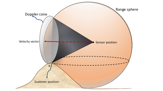
Figure 2: The SAR image of a scatterer is reconstructed at the intersection of the iso-range (sphere) and iso-Doppler (cone) surfaces and the height of the scatterer.

More precisely, the image of a scatterer is formed at $\bi z$ satisfying the following equations:

$$\textmd{Iso-range}\ \textmd{surface:}\qquad\qquad\ \ |\mathbf{z}-\bm{\gamma}_{i}(s)| =R_{i}(\mathbf{x},s)$$ (11)

$$\textmd{Iso-Doppler}\ \textmd{surface:}\quad\widehat{(\mathbf{z}-\bm{\gamma}_{i}(s))}\cdot\dot{\bm{\gamma}}_{i}(s) =\partial_{s}R_{i}(\mathbf{x},s)$$ (12)

$$\textmd{Height:}\qquad\qquad\qquad\qquad\qquad\qquad\ z_{3} =h(\bi x),\ \ \mathbf{z}=[\bi z,z_{3}].$$ (13)

Note that $R_{i}(\mathbf{x},s)$ and $\partial_{s}R_{i}(\mathbf{x},s)$ are the measured range and Doppler and $h(\bi x)$ is the height of the scatterer. As functions of $\mathbf{z}$, (11) and (12) define the iso-range and iso-Doppler surfaces, respectively.

Iso-range contours are defined as the intersection of the iso-range surface, i.e., sphere, and the ground topography. Without loss of generality, we consider a filtered backprojection (FBP) type method where the received and demodulated signals are backprojected onto iso-range contours defined on a reference surface [31], [29]. In the absence of heigh information, demodulated signal is backprojected onto the intersection of the iso-range surface and a known reference surface. Without loss of generality, we assume a flat reference surface at zero height and backproject the demodulated signals onto the following iso-range contours:

$$H^{Range}_{i}(\mathbf{z}_{0})=\left\{\mathbf{z}_{0}\in\left.\mathbb{R}^{3}\ \right|\ \mathbf{z}_{0}=[\bi z,\ 0]\ \textrm{and}\ |\mathbf{z}_{0}-\bm{\gamma}_{i}(s)|=R_{i}(\brmn x,s)\right\}.$$ (14)

Let $\mathcal{K}_{i}^{WB}$ be an FBP operator. Then, the reconstructed image of the scatterer at $\mathbf{x}$ becomes

$$I_{i}^{WB}(\brmn z_{0}^{i}) := \mathcal{K}_{i}^{WB}[\tilde{d}_{i}^{WB}](\brmn z_{0}^{i}),$$ (15)

$$= \int{\mathrm{e}}^{{\mathrm{i}}\omega^{\prime}(t-2R_{i}(\mathbf{z}_{0}^{i},s)/c)}Q_{i}^{WB}(\bi z_{0}^{i},\omega^{\prime},s){d}_{i}^{WB}(t,s){\mathrm{d}}\omega^{\prime}{\mathrm{d}}t{\mathrm{d}}s,$$ (16)

where $Q_{i}^{WB}$ is a filter that can be chosen with respect to a variety of criteria [31], [34].

From (10), the image of the scatterer at $\mathbf{x}$ becomes

$$I_{i}^{WB}(\brmn z_{0}^{i})=|I_{i}^{WB}(\brmn z_{0}^{i})|{\mathrm{e}}^{{\mathrm{i}}2\frac{\omega_{0}}{c}R_{i}(\brmn x,s_{0}^{i})}.$$ (17)

The magnitude of reconstructed images is a measure of target reflectivity, whereas the phase of the reconstructed image depends on the true location, $\mathbf{x}=[\bi x,\ h(\bi x)]$ of the scatterer. However, since the true height $h(\bi x)$ of the scatter is unknown and hence different than that of the reference surface, the location, $\bi z_{0}^{i}$, at which the scatterer is reconstructed is different than its true location, $\bi x$. This positioning error due to incorrect height information is known as layover. Fig. 3 depicts the layover effect.

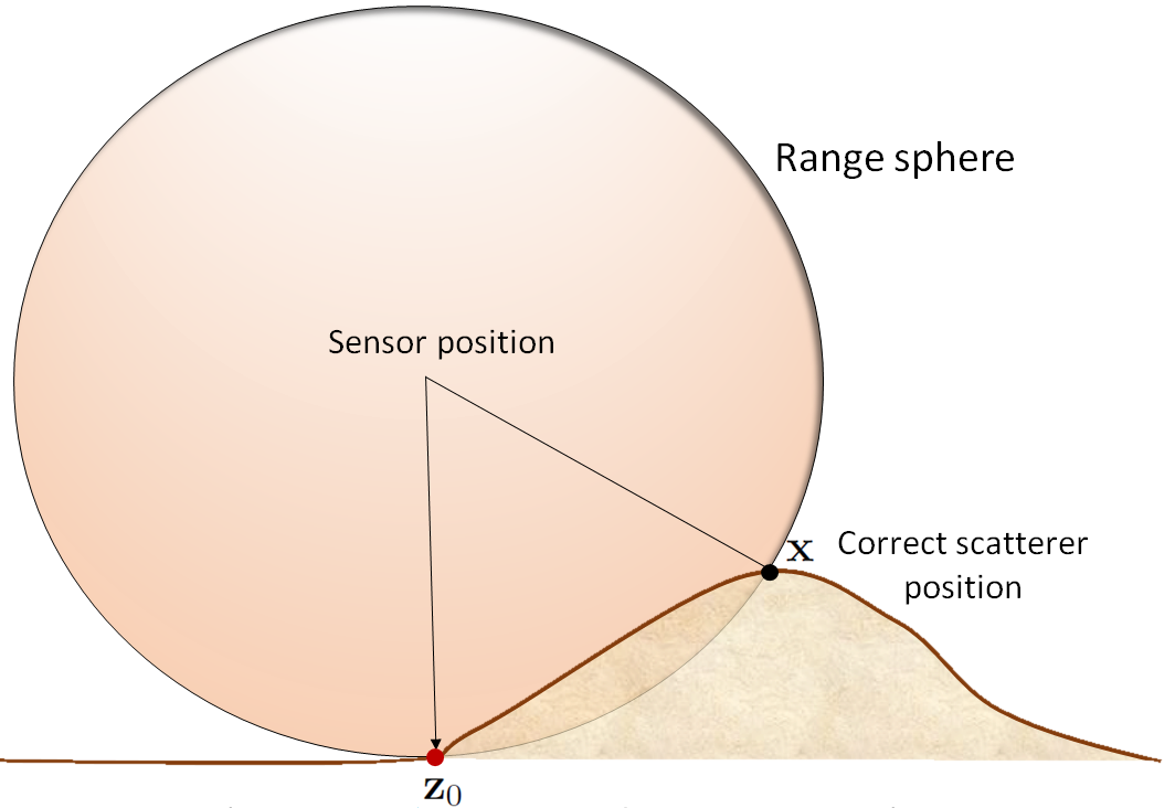
Figure 3: Layover in wideband SAR - The range sphere depicts the iso-range surface of the monostatic SAR configuration. Since the correct height of the scatterer at location $\mathbf{x}$ is unknown, the image of the scatterer at $\mathbf{x}$ is formed at $\mathbf{z}_{0}$ on a flat surface.

We see that without the knowledge of ground topography, additional information or measurements are needed to reconstruct the scatterers at correct locations. This additional information is provided by a second antenna that has a different vantage point than the first one.

3.3 Wideband SAR interferometric height reconstruction

An interferogram is formed by multiplying one of the SAR images with the complex conjugate of the other SAR image [9, 10]. Prior to multiplying the SAR images, the two intensity images, $|I_{i}^{WB}(\brmn z_{0}^{i})|$, $i=1,2$ are co-registered so that pixel locations $\bi z_{0}^{1}$ and $\bi z_{0}^{2}$, each corresponding to the scatterer at position $\mathbf{x}$ in the scene, are roughly aligned. Multiplying $I_{1}^{WB}(\brmn z_{0}^{1})$ with the complex conjugate of $I_{2}^{WB}(\brmn z_{0}^{2})$, we get

$$I_{1}^{WB}(\brmn z_{0}^{1})\overline{I_{2}^{WB}(\brmn z_{0}^{2})}=|I_{1}^{WB}(\brmn z_{0}^{1})||I_{2}^{WB}(\brmn z_{0}^{2})|\mathrm{e}^{\mathrm{i}2\frac{\omega_{0}}{c}(R_{1}(\brmn x,s_{0}^{1})-R_{2}(\brmn x,s_{0}^{2}))}.$$ (18)

We refer to the phase of the interferogram as the wideband interferometric phase

$$\Phi^{WB}_{s_{0}}(\mathbf{x}) = 2\frac{\omega_{0}}{c}(R_{1}(\brmn x,s_{0}^{1})-R_{2}(\brmn x,s_{0}^{2}))$$ (19)

where $s_{0}$ is a multi-index for $\{s_{0}^{1},s_{0}^{2}\}$. The interferometric phase $\Phi^{WB}_{s_{0}}$ provides us the third measurement needed to determine the location of a scatterer in $\mathbb{R}^{3}$. In general the range difference can be many multiples of $2\pi$. Unique phase proportional to range difference can be determined by a phase unwrapping process [1].

Now consider the following surface

$$|\mathbf{z}-\bm{\gamma}_{1}(s_{0}^{1})|-|\mathbf{z}-\bm{\gamma}_{2}(s_{0}^{2})|=\frac{c}{2\omega_{0}}\Phi^{WB}_{s_{0}}(\mathbf{x})$$ (20)

where $\Phi^{WB}_{s_{0}}(\mathbf{x})$ is the measured interferometric phase. (20) defines a two-sheet hyperboloid with foci at $\bm{\gamma}_{1}(s_{0}^{1})$ and $\bm{\gamma}_{2}(s_{0}^{2})$. We assume that the distance between the antennas is much smaller than the ranges of the antennas to the scene and approximate this hyperboloid as follows:

$$\brmn L_{1}(\brmn z,s_{0}^{1})\cdot\brmn b\approx\frac{c}{2\omega_{0}}\Phi^{WB}_{s_{0}}(\mathbf{x})$$ (21)

where

$$\brmn b=\bm{\gamma}_{2}(s_{0}^{2})-\bm{\gamma}_{1}(s_{0}^{1})$$ (22)

is the baseline vector. (21) defines a cone whose vertex is the first antenna and the axis of rotation is the baseline vector. We call this surface the interferometric phase cone. The interferometric phase cone provides the third equation needed to locate the position of a scatterer in $\mathbb{R}^{3}$. More precisely, the location of the scatterer is given by the solution of the following equations:

$$\textmd{Range}\ \textmd{sphere:}\qquad\qquad\qquad\ \ |\mathbf{z}-\bm{\gamma}_{1}(s_{0}^{1})| =R_{1}(\mathbf{x},s_{0}^{1})$$ (23)

$$\textmd{Doppler}\ \textmd{cone:}\qquad\ \ \ \widehat{(\mathbf{z}-\bm{\gamma}_{1}(s_{0}^{1}))}\cdot\dot{\bm{\gamma}}_{1}(s_{0}^{1})) =\left.\partial_{s}R_{1}(\mathbf{x},s)\right|_{s=s_{0}^{1}}$$ (24)

$$\textmd{Interferometric}\ \textmd{phase}\ \textmd{cone:}\quad\brmn L_{1}(\brmn z,s_{0}^{1})\cdot\brmn b =\frac{c}{2\omega_{0}}\Phi^{WB}_{s_{0}}(\mathbf{x}).$$ (25)

The right-hand-side of (23)-(25) are measured quantities defined in terms of the true location, $\mathbf{x}$, of the scatterer in the scene and the left hand-side-defines the three surfaces in terms of the location of the scatterer $\mathbf{z}$ in the image. Fig. 4 geometrically illustrates the solution of these three equations in wideband SAR interferometry.

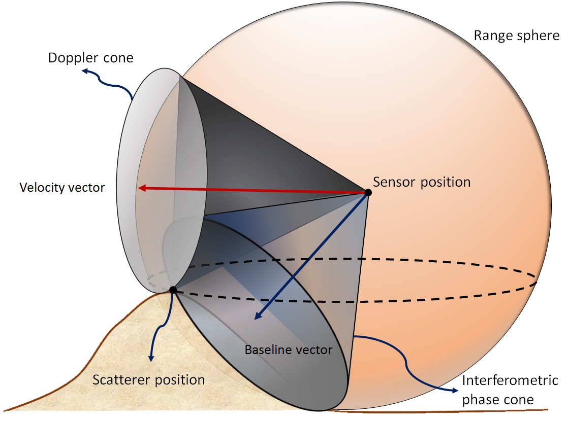
Figure 4: Wideband SAR interferometry provides a third algebraic equation by which the unknown location of a scatters in $\mathbb{R}^{3}$ is determined. The scatterer is located at the intersection of the Doppler-cone, iso-range sphere, and the interferometric phase cone. The axis of rotation of the Doppler-cone is the velocity of the first antenna and the axis of rotation of the interferometric cone is the baseline vector extending from the first to the second antenna.

Typically the variation in the color coding of interferogram is “flattened” by subtracting the expected phase from a surface of constant elevation. Let $\brmn x=\brmn l+\brmn z_{0}$. Then, under the assumption that $|\mathbf{l}|\ll|\mathbf{z}_{0}-\bm{\gamma}_{1}(s)|$

$$\widehat{(\mathbf{x}-\bm{\gamma}_{1}(s))} \approx \widehat{(\mathbf{z}_{0}-\bm{\gamma}_{1}(s))}+\frac{\mathbf{l}_{1}^{\bot}}{|\mathbf{z}_{0}-\bm{\gamma}_{1}(s)|}$$ (26)

where

$$\mathbf{l}_{1}^{\bot}=\mathbf{l}-\widehat{(\mathbf{z}_{0}-\bm{\gamma}_{1}(s))}\left[\frac{\mathbf{l}\cdot\widehat{(\mathbf{z}_{0}-\bm{\gamma}_{1}(s))}}{|\mathbf{z}_{0}-\bm{\gamma}_{1}(s)|}\right].$$ (27)

In other words, the vector $\mathbf{l}_{1}^{\bot}$ is the component of $\mathbf{l}$ perpendicular to $\widehat{(\mathbf{z}_{0}-\bm{\gamma}_{1}(s))}$. The flattened phase then becomes

$$\Phi_{flat}^{WB}(\mathbf{x}) = 2\frac{\omega_{0}}{c}\left[\mathbf{L}_{1}(\mathbf{x},s_{0}^{1})-\mathbf{L}_{1}(\mathbf{z}_{0},s_{0}^{1})\right]\cdot\mathbf{b}$$ (28)

$$\approx 2\frac{\omega_{0}}{c}\frac{\mathbf{l}_{1}^{\bot}\cdot\mathbf{b}}{R(\mathbf{z}_{0},s_{0}^{1})}.$$ (29)

Since $\mathbf{b}_{1}^{\perp}\cdot\mathbf{l}=\mathbf{l}_{1}^{\perp}\cdot\mathbf{b}$ where $\mathbf{b}_{1}^{\perp}$ is the component of $\mathbf{b}$ perpendicular to $\mathbf{L}_{1}(\mathbf{z},s_{0}^{1})$, (29) can be alternatively expressed as

$$\Phi_{flat}^{WB}(\mathbf{x})=2\frac{\omega_{0}}{c}\frac{\mathbf{b}_{1}^{\bot}\cdot\mathbf{l}}{R(\mathbf{z}_{0},s_{0}^{1})}.$$ (30)

Fig. 5 illustrates the key concepts and vectors involved in the wideband interferometry.

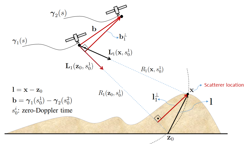
Figure 5: A two-dimensional illustration of vectors involved in wideband interferometric phase. $\brmn l=\brmn x-\brmn z_{0}$ where $\brmn z_{0}=[\bi z_{0},0]$, $\bm{\gamma}_{i}(s_{0}^{i})$ denotes the location of the $i^{th}$ antenna at the zero-Doppler time $s_{0}^{i}$, $\brmn L_{1}(\brmn z_{0},s_{0}^{1})$ denotes the look-direction of the first antenna with respect to the reference scatterer located at $\mathbf{z}_{0}$, and $\brmn l^{\perp}_{1}$ is the component of $\brmn l$ perpendicular to $\mathbf{L}_{1}(\brmn z_{0},s_{0}^{1})$. The wideband interferometric phase is related to the projection of the baseline vector, $\brmn b$, onto the the look-direction, $\brmn L_{1}(\brmn x,s_{0}^{1})$, of the antenna with respect to scatterer location $\mathbf{x}$. Known vectors are shown in red and unknown vectors are shown in black.

4 Data Model and Image Formation for Doppler-SAR

4.1 Data Model for Doppler-SAR

We consider two mono-static antennas following the trajectories $\bm{\gamma}_{i}(t)$, $i=1,2$, transmitting ultra-narrowband CWs as shown in Fig. 1. Let $p(t)\approx\tilde{p}(t){\mathrm{e}}^{{\mathrm{i}}\omega_{0}}$ be the transmitted waveform where $\omega_{0}$ is the center frequency. The scattered field model at the $i^{\textmd{th}}$ antenna is then given by

$$r_{i}(t)=\frac{\omega_{0}^{2}}{(4\pi)^{2}}\int\frac{{\mathrm{e}}^{-{\mathrm{i}}\omega_{0}(t-2|\mathbf{x}-\bm{\gamma}_{i}(t)|/c)}}{|\brmn x-\bm{\gamma}_{i}(t)|^{2}}\tilde{p}(t-2|\mathbf{x}-\bm{\gamma}_{i}(t)|/c)V(\brmn x){\mathrm{d}}\brmn x.$$ (31)

Let $\mu\in\mathbb{R}^{+}$ and $\phi(t)$ be a smooth windowing function with a finite support, $t\in[0,T_{\phi}]$. Following [15, 14, 23], we correlate $r_{i}(t)$ with a scaled and translated version of the transmitted signal over $\phi(t)$ as follows:

$$d_{i}^{UNB}(\mu,s)=\int r_{i}(t){\mathrm{e}}^{{\mathrm{i}}\omega_{0}\mu(t-sT_{\phi})/c}\tilde{p}^{*}(\mu(t-sT_{\phi}))\phi(t-sT_{\phi}){\mathrm{d}}t.$$ (32)

Inserting (31) into (32), we obtain

$$d_{i}^{UNB}(\mu,s)=\frac{\omega_{0}^{2}}{(4\pi)^{2}} \int\frac{{\mathrm{e}}^{-{\mathrm{i}}\omega_{0}(t-2|\mathbf{x}-\bm{\gamma}_{i}(t)|/c)}}{|\brmn x-\bm{\gamma}_{i}(t)|^{2}}\tilde{p}(t-2|\mathbf{x}-\bm{\gamma}_{i}(t)|/c)V(\brmn x)$$ (33)

$$\quad\times{\mathrm{e}}^{{\mathrm{i}}\omega_{0}\mu(t-sT_{\phi})/c}\tilde{p}^{*}(\mu(t-sT_{\phi}))\phi(t-sT_{\phi}){\mathrm{d}}t{\mathrm{d}}\brmn x.$$ (34)

Approximating $\bm{\gamma}_{i}(t)$ around $t=sT_{\phi}$, $\bm{\gamma}_{i}(t)\approx\bm{\gamma}_{i}(sT_{\phi})+\dot{\bm{\gamma}}_{i}(sT_{\phi})(t-sT_{\phi})$, and making the far-field approximation, we write

$$|\brmn x-\bm{\gamma}_{i}(t)|\approx|\brmn x-\bm{\gamma}_{i}(sT_{\phi})|-\brmn L_{i}(\brmn x,sT_{\phi})\cdot\dot{\bm{\gamma}}_{i}(sT_{\phi})(t-sT_{\phi}),$$ (35)

where $\brmn L_{i}(\brmn x,sT_{\phi})=\widehat{(\brmn x-\bm{\gamma}_{i}(sT_{\phi}))}$ and $\dot{\bm{\gamma}}_{i}(sT_{\phi})=\partial_{s}\bm{\gamma}_{i}(sT_{\phi})$ is the velocity of the $i^{\textmd{th}}$ antenna.

To simplify our notation, for the rest of the paper, we set $\brmn L_{i}(\brmn x,sT_{\phi})=\brmn L_{i}(\brmn x,s)$, $\bm{\gamma}_{i}(sT_{\phi})=\bm{\gamma}_{i}(s)$, $\dot{\bm{\gamma}}_{i}(sT_{\phi})=\dot{\bm{\gamma}}_{i}(s)$, $\partial_{s}^{2}\bm{\gamma}_{i}(sT_{\phi})=\ddot{\bm{\gamma}}_{i}(sT_{\phi})=\ddot{\bm{\gamma}}_{i}(s)$ and $R_{i}(\mathbf{x},sT_{\phi})=R_{i}(\mathbf{x},s)$. We next define Doppler for the $i^{\textmd{th}}$ antenna

$$f_{i}^{d}(\brmn x,s)=-\frac{\omega_{0}}{c}\brmn L_{i}(\brmn x,s)\cdot\dot{\bm{\gamma}}_{i}(s).$$ (36)

Inserting (35) and (33) into (36), the data model becomes

$$d_{i}^{UNB}(\mu,s)=\int{\mathrm{e}}^{-{\mathrm{i}}t[\omega_{0}(1-\mu)-2f_{i}^{d}(\brmn x,s)]}\tilde{A}_{i}(t,\brmn x,s,\mu){\mathrm{e}}^{{\mathrm{i}}2f_{i}^{d}(\brmn x,s)sT_{\phi}}V(\brmn x){\mathrm{d}}t{\mathrm{d}}\brmn x,$$ (37)

where $\tilde{A}_{i}(t,\brmn x,s,\mu)$ is a slow varying function of $t$ composed of the rest of the terms in (33).

We now approximate $f_{i}^{d}(\brmn x,s)$ around $s=s_{d}^{i}$ as follows:

$$f_{i}^{d}(\brmn x,s)\approx f_{i}^{d}(\brmn x,s_{d}^{i})+(s-s_{d}^{i})\left.\partial_{s}f_{i}^{d}(\brmn x,s)\right|_{s=s_{d}^{i}}+\frac{(s-s_{d}^{i})^{2}}{2}\left.\partial^{2}_{s}f_{i}^{d}(\brmn x,s)\right|_{s=s_{d}^{i}}.$$ (38)

We choose $s_{d}^{i}$ such that

$$\left.\frac{\partial f_{i}^{d}(\brmn x,s)}{\partial s}\right|_{s=s_{d}^{i}}=0\quad\Rightarrow\quad\brmn L_{i}(\brmn x,s_{d}^{i})\cdot\ddot{\bm{\gamma}}_{i}(s_{d}^{i})-\frac{\dot{\bm{\gamma}}_{i}(s_{d}^{i})\cdot\dot{\bm{\gamma}}_{i}^{\perp}(s_{d}^{i})}{R_{i}(\mathbf{x}s_{d}^{i})}=0$$ (39)

where $\ddot{\bm{\gamma}}_{i}(s_{d}^{i})$ is the acceleration of the $i^{\textmd{th}}$ antenna and $\dot{\bm{\gamma}}_{i}^{\perp}(s_{d}^{i})$ is the component of $\dot{\bm{\gamma}}_{i}(s_{d}^{i})$ perpendicular to the look-direction $\brmn L_{i}(\brmn x,s_{d}^{i})$ as described in (27). We refer to $s_{d}^{i}$ as the zero-Doppler-rate time for the $i^{\textmd{th}}$ antenna.

Using (38) in ${\mathrm{e}}^{{\mathrm{i}}2f_{i}^{d}(\brmn x,s)sT_{\phi}}$ and redefining the slow-varying function in $t$,

$$A_{i}(t,\brmn x,s,\mu)=\tilde{A}_{i}(t,\brmn x,s,\mu){\mathrm{e}}^{{\mathrm{i}}2s_{d}^{i}T_{\phi}\frac{(s-s_{d}^{i})^{2}}{2}\partial^{2}_{s}f_{i}^{d}(\brmn x,s)|_{s=s_{d}^{i}}},$$ (40)

we obtain the following data model for Doppler-SAR image reconstruction:

$$d_{i}^{UNB}(\mu,s)\approx\int{\mathrm{e}}^{-{\mathrm{i}}t[\omega_{0}(1-\mu)-2f_{i}^{d}(\brmn x,s)]}A_{i}(t,\brmn x,s,\mu){\mathrm{e}}^{{\mathrm{i}}2f_{i}^{d}(\brmn x,s_{d}^{i})s_{d}^{i}T_{\phi}}V(\brmn x){\mathrm{d}}t{\mathrm{d}}\brmn x.$$ (41)

4.2 Doppler-SAR Image Formation and Layover

Similar to the wideband case, we reconstruct images by backprojection as described in [35, 15] [14]. The forward model in (41) shows that the data, $d_{i}^{UNB}(s,\mu)$, is the weighted integral of the scene reflectivity over iso-Doppler contours. It was shown in [14] that a scatterer located at $\mathbf{x}$ in the scene is reconstructed at the intersection of iso-Doppler surface and iso-Doppler-rate surface and ground topography. More precisely, the image of a scatterer located at $\mathbf{x}$ in the scene is reconstructed at $\bi z$ satisfying the following equations:

$$\qquad\textmd{Iso-Doppler}\ \textmd{surface:}\qquad\qquad\qquad\qquad\ \ \ \ \mathbf{L}_{i}^{d}(\mathbf{z},s)\cdot\dot{\bm{\gamma}}_{i}(s) =\frac{c}{\omega_{0}}f_{i}^{d}(\mathbf{x},s)$$ (42)

$$\qquad\textmd{Iso-Doppler-rate}\ \textmd{surface:}\quad\mathbf{L}_{i}(\mathbf{z},s)\cdot\ddot{\bm{\gamma}}_{i}(s)-\frac{\dot{\bm{\gamma}}_{i}(s)\cdot\dot{\bm{\gamma}}_{i}^{\perp}(s)}{R_{i}(\mathbf{z},s)} =\frac{c}{\omega_{0}}\partial_{s}f_{i}^{d}(\mathbf{x},s)$$ (43)

$$\qquad\textmd{Height:}\qquad\qquad\qquad\qquad\qquad\qquad\qquad\qquad\qquad\ \ \ \ z_{3} =h(\bi x),\ \ \mathbf{z}=[\bi z,z_{3}]$$ (44)

where the right-hand-side of (42)-(43) corresponds to measurements and the left-hand-side defines surfaces in image parameter $\mathbf{z}$.

The iso-Doppler-rate surface, given by the following set,

$$\qquad H^{Dop-rate}_{i}(\mathbf{z})=\left\{\mathbf{z}\in\left.\mathbb{R}^{3}\ \right|\ \brmn L_{i}(\mathbf{z},s)\cdot\ddot{\bm{\gamma}}_{i}(s)-\frac{\dot{\bm{\gamma}}_{i}(s)\cdot\dot{\bm{\gamma}}_{i}^{\perp}(s)}{R_{i}(\mathbf{z},s)}=\frac{c}{\omega_{0}}\partial_{s}f_{i}^{d}(\mathbf{x},s)\right\}.$$ (45)

can be viewed as a continuum of intersections of cones and expanding spheres centered at the sensor location. The axis of rotation for the surface is the acceleration vector of the antenna trajectory. Fig. 6 illustrates iso-Doppler and iso-Doppler-rate surfaces and the reconstruction of a point scatterer by the intersection of these surfaces and ground topography. The reconstruction is analogous to the wideband SAR image reconstruction shown in Fig. 2.

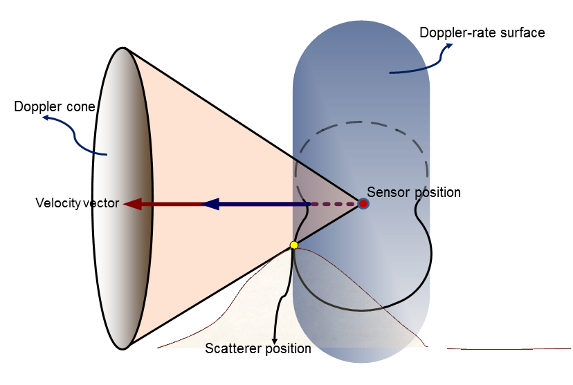
Figure 6: In Doppler-SAR image reconstruction, a scatterer located at $\mathbf{x}$ in the scene is correctly reconstructed at the intersection of the iso-Doppler and iso-Doppler-rate surfaces and the ground topography. Iso-Doppler surface is a cone in which its vertex is the antenna location and its axis of rotation is the antenna velocity. The geometry of the iso-Doppler-rate surface depends on the antenna trajectory. Figure is drawn for a linear trajectory at a constant height.

In the absence of ground topography information, we backproject data onto iso-Doppler contours on a reference surface. Without loss of generality, we consider the following iso-Doppler contours:

$$\qquad\qquad H^{Dop}_{i}(\mathbf{z}_{0})=\left\{\mathbf{z}_{0}\in\left.\mathbb{R}^{3}\ \right|\ \mathbf{z}_{0}=[\bi z,\ 0]\ \textrm{and}\ \brmn L_{i}(\brmn z,s)\cdot\dot{\bm{\gamma}}_{i}(s)=\frac{c}{\omega_{0}}f_{i}^{d}(\brmn x,s)\right\}$$ (46)

where the right-hand-side of the equality in (46) is the high resolution measurement provided by ultra-narrowband CW.

Let $\mathcal{K}_{i}^{UNB}$ be an FBP operator as described in [14]. Then, the reconstructed image is given by:

$$I^{UNB}_{i}(\brmn z_{0}^{i}) := \mathcal{K}_{i}^{UNB}[d^{UNB}_{i}](\brmn z_{0}^{i})$$ (47)

$$\approx \int{\mathrm{e}}^{{\mathrm{i}}t(\omega_{0}(1-\mu)-2f_{i}^{d}(\mathbf{z}_{0}^{i},s))}Q^{UNB}_{i}(s,\bi z_{0}^{i},t)d^{UNB}_{i}(s,\mu){\mathrm{d}}t{\mathrm{d}}\mu{\mathrm{d}}s$$ (48)

where $Q^{UNB}_{i}$ is a filter that can be chosen as in [35, 15, 14]. The reconstructed image is given by

$$I_{i}^{UNB}(\brmn z_{0}^{i})=|I_{i}^{UNB}(\brmn z_{0}^{i})|{\mathrm{e}}^{{\mathrm{i}}2f_{i}^{d}(\brmn x,s_{d}^{i})s_{d}^{i}T_{\phi}}.$$ (49)

In the absence of topography information, we see that a scatterer located at $\mathbf{x}$ in the scene is reconstructed at $\mathbf{z}_{0}^{i}\neq\mathbf{x}$ in the image. This position error in the reconstructed image is the counterpart of the layover effect observed in conventional wideband SAR images. Fig. 7 illustrates the layover effect in Doppler-SAR. However, the phase of the reconstructed image is a function of the scatterer’s true location, $\mathbf{x}$, and hence, includes its height information, $h(\bi x)$.

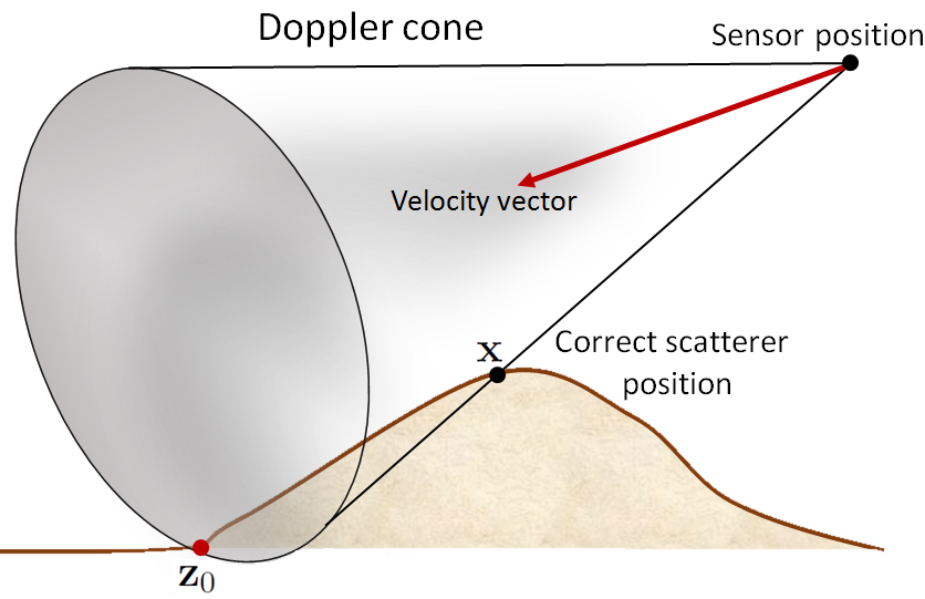
Figure 7: If the height of a scatter is not known, it is reconstructed at an incorrect position. Both the correct scatterer location $\mathbf{x}$ and its image $\mathbf{z}_{0}$ lie on the same iso-Doppler surface, i.e., the Doppler cone. $\brmn z_{0}$ lies at the intersection of the Doppler cone defined $f_{1}^{d}(\brmn x,s)$ and the flat topography.

Note that the phases of the reconstructed images depend on the Doppler-rate, $f_{i}^{d}(\brmn x,s_{d}^{i})$, the duration of the windowing function, $T_{\phi}$, and the corresponding zero-Doppler-rate times, $s_{d}^{i}$. The height information is included in the Doppler-rate. However, since each imaging geometry may yield different zero-Doppler-times, Doppler-rate in the phase of each image is multiplied by a different zero-Doppler-rate time. To equalize the effect of this multiplication factor, we multiply one of the reconstructed images with itself so that the Doppler-rate in the phase of both images are multiplied by the same factor, say $s_{d}^{1}$. As a result, each image becomes

$$I_{i}^{UNB}(\brmn z_{0}^{i})=|I_{i}^{UNB}(\brmn z_{0}^{i})|{\mathrm{e}}^{{\mathrm{i}}2f_{i}^{d}(\brmn x,s_{d}^{i})s_{d}^{1}T_{\phi}},\quad i=1,2.$$ (50)

5 Doppler-SAR Interferometric Height Reconstruction

Similar to the wideband case, we form two Doppler-SAR images, $I_{i}^{UNB}(\brmn z_{0}^{i})$, $i=1,2$, co-register the intensity images $|I_{i}^{WB}(\brmn z_{0}^{i})|$ and multiply one of them by the complex conjugate of the other to form an interferogram. Then the interferometric phase, i.e., the phase function of $I_{1}^{UNB}(\brmn x)\overline{I_{2}^{UNB}(\brmn x)}$ is given by

$$\Phi^{UNB}_{s_{d}}(\brmn x)=2s_{d}^{1}T_{\phi}\left(f_{1}^{d}(\brmn x,s_{d}^{1})-f_{2}^{d}(\brmn x,s_{d}^{2})\right)$$ (51)

where $s_{d}$ denotes multi-index for $\{s_{d}^{1},s_{d}^{2}\}$. Thus the scatterer lies on the following surface:

$$\mathbf{L}_{1}(\mathbf{z},s_{d}^{1})\cdot\dot{\bm{\gamma}}_{1}(s_{d}^{1})-\mathbf{L}_{2}(\mathbf{z},s_{d}^{2})\cdot\dot{\bm{\gamma}}_{2}(s_{d}^{2})=-\frac{c}{2\omega_{0}}\left(f_{1}^{d}(\brmn x,s_{d}^{1})-f_{2}^{d}(\brmn x,s_{d}^{2})\right)$$ (52)

where the right-hand-side is the measured interferometric phase. The left-hand-side of (52) defines a surface that can be described as the intersections of two cones one of which has a continuously changing solid angle.

Assuming that the distance between the antennas is much smaller than the ranges of the antennas to the scene, we can approximate the look-direction of the second antenna in terms of the look-direction of the first one as follows:

$$\mathbf{L}_{2}(\mathbf{x},s_{d}^{2})=\mathbf{L}_{1}(\mathbf{x},s_{d}^{1})+\frac{\mathbf{b}_{1}^{\perp}}{R_{1}(\mathbf{x},s_{d}^{1})}$$ (53)

where $\mathbf{b}=\bm{\gamma}_{2}(s_{d}^{2})-\bm{\gamma}_{1}(s_{d}^{1})$ is the baseline vector and $\mathbf{b}_{1}^{\perp}$ is the component of $\mathbf{b}$ perpendicular to the look-direction of the first antenna. Using (53), we approximate the interferometric phase as follows:

$$-\frac{c}{2s_{d}^{1}T_{\phi}\omega_{0}}\Phi^{UNB}_{s_{d}}(\brmn x)\approx\mathbf{L}_{1}(\mathbf{x},s_{d}^{1})\cdot\mathbf{v}+\frac{\mathbf{b}_{1}^{\perp}\cdot\dot{\bm{\gamma}}_{2}(s_{d}^{2})}{R_{1}(\mathbf{x},s_{d}^{1})}$$ (54)

where

$$\mathbf{v}=\dot{\bm{\gamma}}_{2}(s_{d}^{2})-\dot{\bm{\gamma}}_{1}(s_{d}^{1}).$$ (55)

We refer to $\mathbf{v}$ as the baseline velocity. We see that (54) approximates the interferometric phase as a Doppler-rate. Additionally, (54) shows that Doppler-SAR interferometry involves not only configuring antennas in position space, but also in velocity space. The larger the difference in antenna velocities in the look-direction of the first antenna, the larger the interferometric phase becomes. If on the other hand, the velocities of the antennas are the same, the second term in (54) defines the interferometric phase surface.

Clearly, in Doppler-SAR interferometry (54) provides the third equation needed to determine the location of a scatterer in $\mathbb{R}^{3}$. More precisely, the location of a scatterer is given by the solution of the following three equations:

$$\textmd{Iso-Doppler:}\qquad\qquad\qquad\qquad\qquad\ \widehat{(\mathbf{z}-\bm{\gamma}_{1}(s_{d}^{1}))}\cdot\dot{\bm{\gamma}}_{1}(s_{d}^{1}) =\frac{c}{\omega_{0}}f_{1}^{d}(\mathbf{x},s_{d}^{1})$$ (56)

$$\textmd{Iso-Doppler-rate:}\ \widehat{(\mathbf{z}-\bm{\gamma}_{1}(s_{d}^{1}))}\cdot\ddot{\bm{\gamma}}_{1}(s_{d}^{1})-\frac{\dot{\bm{\gamma}}_{1}(s_{d}^{1})\cdot\dot{\bm{\gamma}}_{1}^{\perp}(s_{d}^{1}T_{\phi})}{R_{1}(s_{d}^{1},\mathbf{z})} =\partial_{s}f_{1}^{d}(\mathbf{x},s_{d}^{1})$$ (57)

$$\textmd{Interferometric Doppler-rate:}\quad\ \mathbf{L}_{1}(\mathbf{z},s_{d}^{1})\cdot\mathbf{v}+\frac{\mathbf{b}_{1}^{\perp}\cdot\dot{\bm{\gamma}}_{2}(s_{d}^{2})}{R_{1}(\mathbf{z},s_{d}^{1})} =-\frac{c}{2s_{d}^{1}T_{\phi}\omega_{0}}\Phi^{UNB}_{s_{d}}(\mathbf{x}).$$ (58)

Fig. (8) depicts the intersection of the three surfaces at the scatterer location in $\mathbb{R}^{3}$.

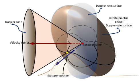
Figure 8: Determination of the scatterer location in Doppler-SAR interferometry. The scatterer is located at the intersection of the Doppler cone and the two iso-Doppler-rate surfaces. Interferometric phase measurement provides the third surface, i.e., the interferometric phase iso-Doppler-rate surface.

Similar to the wideband SAR interferometry, the interferometric phase can be “flattened” by subtracting the phase due to a scatterer with known height. Without loss of generality, let $\mathbf{z}_{0}=[\bi z,0]$ with $R_{1}(\mathbf{z}_{0},s)=R_{1}(\mathbf{x},s)$ and $\mathbf{x}=\mathbf{z}_{0}+\mathbf{l}$. Thus, identifying the location of a scatterer is equivalent to determining $\mathbf{l}$.

Using (26), we see that

$$\Phi_{flat}^{UNB}(\mathbf{x})=\Phi_{s_{d}}^{UNB}(\mathbf{x})-\Phi_{s_{d}}^{UNB}(\mathbf{z}_{0})\approx\frac{\mathbf{l}_{1}^{\perp}\cdot\mathbf{v}}{R_{1}(\mathbf{z}_{0},s_{d}^{1})}+\mathcal{O}\left(\frac{1}{R_{1}^{2}(\mathbf{z}_{0},s_{d}^{1})}\right)$$ (59)

where $\mathbf{l}_{1}^{\perp}$ is the component of $\mathbf{l}$ perpendicular to $\mathbf{L}_{1}(\mathbf{z}_{0},s_{d}^{1})$. (59) shows that the flattened interferometric phase for Doppler-SAR interferometry is related to the projection of the unknown $\mathbf{l}_{1}^{\perp}$ onto the baseline velocity vector scaled by the range of the first antenna to $\mathbf{z}_{0}$. Since $\mathbf{l}_{1}^{\perp}\cdot\mathbf{v}=v_{1}^{\perp}\cdot\mathbf{l}$ where $v_{1}^{\perp}$ is the component of $\mathbf{v}$ perpendicular to $\mathbf{L}_{1}(\mathbf{z}_{0},s_{d}^{1})$, we alternative express (59) as follows:

$$\Phi_{flat}^{UNB}(\mathbf{x})\approx\frac{\mathbf{v}_{1}^{\perp}\cdot\mathbf{l}}{R_{1}(\mathbf{z}_{0},s_{d}^{1})}.$$ (60)

Fig. 9 shows the key concepts and vectors involved in Doppler-SAR interferometry.

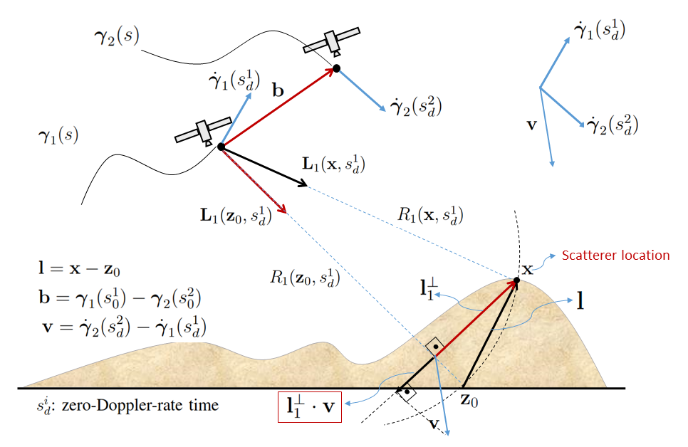
Figure 9: An illustration of key concepts and vectors in Doppler-SAR interferometry. $\brmn l=\brmn x-\brmn z_{0}$ where $\brmn z_{0}=[\bi z_{0},0]$, $\bm{\gamma}_{i}(s)$ denotes the $i^{\textmd{th}}$ antenna position, $\brmn L_{1}(\brmn z_{0},s_{d}^{1})$ denotes the look-direction with respect to a reference surface, $\brmn l^{\perp}_{1}$ is the component of $\brmn l$ perpendicular to $\brmn L_{1}(\brmn z_{0},s_{d}^{1})$, $\dot{\bm{\gamma}}_{1}(s)$ denotes the antenna velocity, $\brmn L_{1}(\brmn x,s_{d}^{1})$ denotes the look-direction of the antenna with respect to the correct target location. Doppler-SAR interferometric phase is proportional to the projection of the baseline velocity vector onto $\brmn l^{\perp}_{1}$. Known vectors are shown in red and unknown vectors are shown in black.

5.1 Comparison of Doppler-SAR Interferometry wide Wideband Case

Table II tabulates the interferometric phase for the wideband SAR and Doppler-SAR cases. We compare and contrast the two interferometric phases below:

• For WB and UNB, the “baseline” is the difference in range and difference in velocity, respectively.

• The larger the $\omega_{0}$, the center frequency, the larger the interferometric phase in both WB and UNB cases.

• The larger the range, $R_{1}$, the smaller the interferometric phase in both WB and UNB cases.

• For UNB, larger the $T_{\phi}$, the larger the interferometric phase.

• For WB, the larger the $\mathbf{b}$, the difference between the positions of the two antennas, the larger the interferometric phase. For UNB, the larger the $\mathbf{v}$, the difference between the velocities of the two antennas, the larger the interferometric phase.

Table 2: Raw and flattened interferometric phase functions for wideband SAR and Doppler-SAR.

	Interferometric Phase	Flattened Interferometric Phase
Wideband SAR	$2\frac{\omega_{0}}{c}\left[\mathbf{L}_{1}(\mathbf{x},s_{0}^{1})\cdot\mathbf{b}\right]$	$2\frac{\omega_{0}}{c}\frac{1}{R_{1}(\mathbf{z}_{0},s_{0}^{1})}\left[\brmn b^{\perp}_{1}\cdot\mathbf{l}\right]$
Doppler-SAR	$-2\frac{\omega_{0}}{c}s_{d}T_{\phi}\left[\mathbf{L}_{1}(\mathbf{x},s_{d}^{1})\cdot\mathbf{v}+\frac{1}{R_{1}(\mathbf{x},s_{d}^{1})}\mathbf{b}_{1}^{\perp}\cdot\dot{\bm{\gamma}}_{2}(s_{d}^{2})\right]$	$-2\frac{\omega_{0}}{c}s_{d}T_{\phi}\frac{1}{R_{1}(\mathbf{z}_{0},s_{d}^{1})}\left[\mathbf{v}_{1}^{\perp}\cdot\mathbf{l}\right]$

6 Numerical Experiments

6.1 Experimental Setup

We conducted numerical experiments for both wideband and Doppler-SAR. Our experimental setup was as follows:

• A scene of size $128\times 128$m at $1$m resolution was imaged.

• A single point target was placed at $(-20,-31,50)$m with the origin $(0,0,0)$ at the scene center.

• Two antennas flying on a linear trajectory parallel to the $y$-axis was used with both antennas placed at $7.1$km from the scene center in the $x$-axis direction. The midpoint of the linear trajectories for both antennas was aligned at $y=0$.

• Wideband: First antenna was placed at height of $3$km and the second at $4$km. The length of the trajectories were $1$km in length for both antennas. Both antennas were moving at velocity of $100$m/s. A waveform with flat spectrum of 100$MHz$ bandwidth at center frequency of $8$GHz was transmitted from both antennas. $512$ frequency samples and $1024$ slow-time, $s$, samples were used for imaging.

• Doppler: First antenna was placed at height of $2$km and the second at $4$km. The length of the trajectories were $1$km for both antennas. The first antenna was moving at velocity of $100$m/s and the second at $400$m/s. A continuous waveform at center frequency of $8$GHz was transmitted from both antennas. A window of $0.01$s was used for processing at each slow time. $512$ fast time, $t$, samples and $1024$ slow-time, $s$, samples were used for imaging.

6.2 Wideband SAR Interferometry

Fig. 10a and Fig. 10b show the reconstructed images of the point target located at $(-20,-31,50)$m from the first and the second antenna, respectively assuming a flat ground topography at height of $0$m.

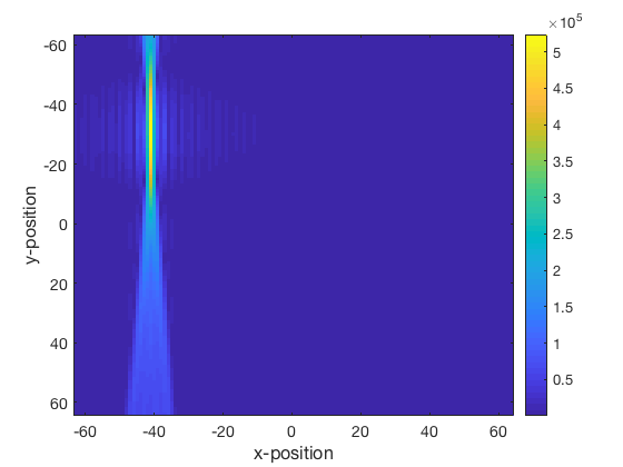
(a)

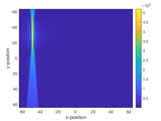
(b)

Figure 10: (a) Wideband reconstruction of the target located at $(-20,-31,50)$m using the first antenna assuming flat ground topography. The target is reconstructed at $(-41,-31,0)$m. (b) Wideband reconstruction of the target located at $(-20,-31,50)$m using the second antenna assuming flat ground topography. The target is reconstructed at $(-48,-31,0)$m.

In both Fig. 10a and Fig. 10b, we see that there is a displacement due to layover effect in the range direction ($x$-axis). The first antenna reconstructs the target at $(-41,-31,0)$m. The second antenna reconstructs the target at $(-48,-31,0)$m.

We next align the peaks in the two images and multiply the first image with the complex conjugate of the second as in (18) to generate the interferogram. The resulting interferogram is shown in Fig. 11.

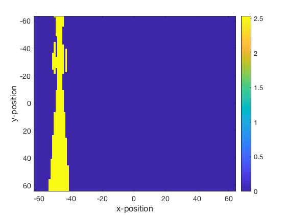
Figure 11: The interferogram from wideband SAR reconstructed images.

In order to reconstruct the height we use the set of equations (23), (24), and (25). The Doppler cone equation (24) at zero-Doppler point $s_{0}^{1}$ gives us that the iso-Doppler contours are in the look-direction, which in our scenario is parallel to the $x$-axis. Thus, iso-Doppler contours have constant $y$ value at the target’s $y$ position. Using this fact, we need only to compute the intersection of iso-range contour (23) and interferometric phase contour (25) fixing the $y$ position. From Figs. 10a and 10b we see that both targets are reconstructed at $y$ position of $-31$m. Thus we reconstruct the true target position using $y=-31$m. For reconstruction, we sampled the height in the interval $[1,100]$m at $0.5$m resolution.

Fig. 12a shows the magnitude image of $|\mathbf{z}-\bm{\gamma}_{1}(s_{0}^{1})|-R_{1}(\mathbf{x},s_{0}^{1})$ at $y=-31$m. Note that $R_{1}(\mathbf{x},s_{0}^{1})$ is the measured value derived from the phase of the reconstructed image. The dark blue area indicates the iso-range contour where the magnitude of the difference is minimized.

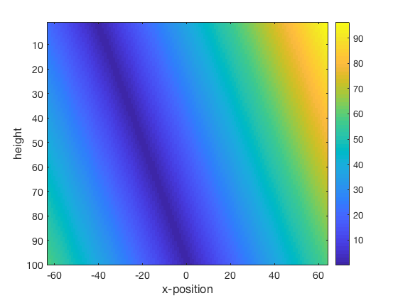
(a)

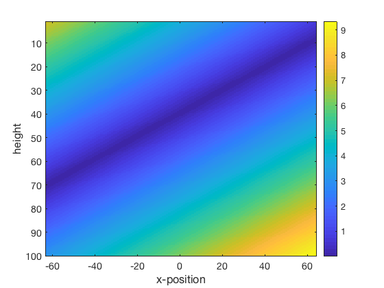
(b)

Figure 12: (a) Image of the magnitude of $|\mathbf{z}-\bm{\gamma}_{1}(s_{0}^{1})|-R_{1}(\mathbf{x},s_{0}^{1})$ at $y=-31$m. The iso-range contour is indicated by dark blue area where the magnitude of $|\mathbf{z}-\bm{\gamma}_{1}(s_{0}^{1})|-R_{1}(\mathbf{x},s_{0}^{1})$ is minimized. (b) Image of the magnitude of $L_{1}(\brmn z,s_{0}^{1})\cdot\brmn b-\frac{c}{2\omega_{0}}\Phi^{WB}_{s_{0}}(\mathbf{x})$ at $y=-31$m. The interferometric phase contour is indicated by dark blue area where the magnitude of $L_{1}(\brmn z,s_{0}^{1})\cdot\brmn b-\frac{c}{2\omega_{0}}\Phi^{WB}_{s_{0}}(\mathbf{x})$ is minimized.

Similarly, Fig. 12b shows the magnitude image of the difference $L_{1}(\brmn z,s_{0}^{1})\cdot\brmn b-\frac{c}{2\omega_{0}}\Phi^{WB}_{s_{0}}(\mathbf{x})$. As before, the dark blue area indicates the interferometric phase contour.

Combining the two images, Fig. 13 shows the intersection of the two contours indicated by the dark blue area. The white ‘x’ in Fig. 13 indicates the exact intersection computed and where the target is reconstructed. The white ‘o’ indicates the true target position. It is clear that the target is reconstructed at the correct position and height.

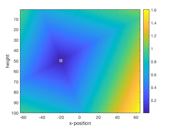
Figure 13: Image of the intersection of the iso-range contour with the interfermetric phase contour at $y=-31$m. The exact intersection is indicated by white ‘x’. The true target position is indicated by white ‘o’. The target is reconstructed at the correct position and height.

6.3 Doppler-SAR

We proceed similar as in the wideband case for the Doppler-SAR case. Figs. 14a and 14b show the reconstructed image for Doppler-SAR for the first and second antennas, respectively.

(a)

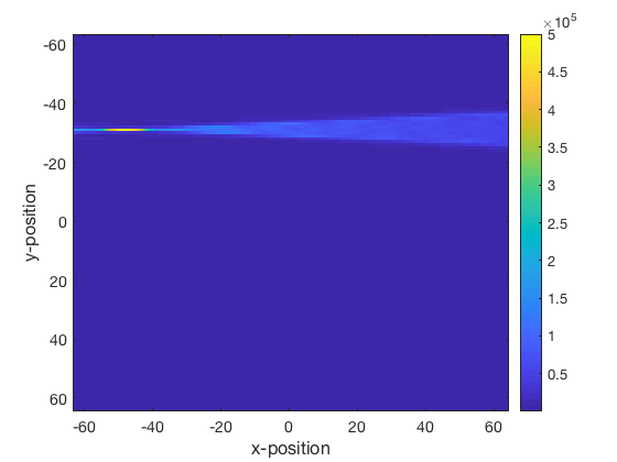
(b)

Figure 14: (a) Doppler-SAR reconstruction of the target located at $(-20,-31,50)$m using the first antenna assuming flat ground topography. The target is reconstructed at $(-34,-31,0)$m. (b) Doppler-SAR reconstruction of the target located at $(-20,-31,50)$m using the second antenna assuming flat ground topography. The target is reconstructed at $(-48,-31,0)$m.

The first antenna reconstructs the target at $(-34,-31,0)$m and the second antenna at $(-48,-31,0)$m.

As in the wideband case, we align the peaks of the two images and multiply the first image with the conjugate of the second image to form the interferogram of the Doppler images. The resulting interferogram is shown in Fig. 15.

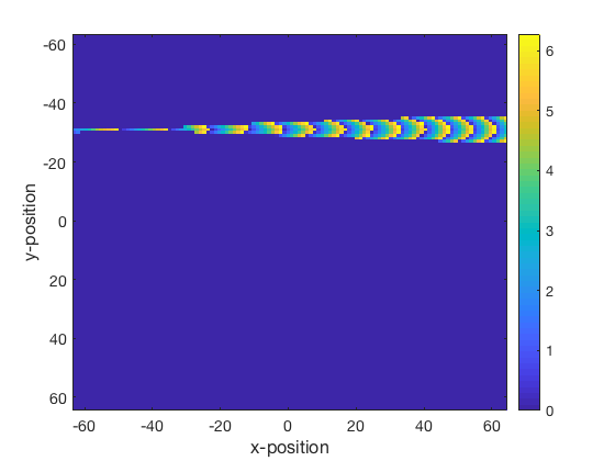
Figure 15: The interferogram from Doppler-SAR reconstructed images.

To reconstruct the height we use the set of equations given in (56), (57), and (58). The zero-Doppler-rate points, $s_{d}^{1}$, is approximated by the end of the antenna’s trajectories farthest from the target position. By (39), for a linear trajectory with constant velocity, true zero-Doppler-rate point would be where $\dot{\bm{\gamma}}_{i}(s_{d}^{1})\perp\dot{\bm{\gamma}}_{i}^{\perp}(s_{d}^{1})$. Namely, where the look-direction is parallel to the velocity vector. The best estimate would be at a point in the trajectory farthest away from the target location.

Fig. 16a illustrates the iso-Doppler surface at $y=-31$m, which is the $y$-position where the target position is reconstructed and the true target’s $y$ position. Notice that both images reconstruct the scatterer at the correct $y$ position. The iso-Doppler contour is given by the dark blue area as before.

Similarly, Figs. 16b and 16c illustrate the iso-Doppler-rate and interferometric Doppler-rate surfaces, respectively at $y=-31$m.

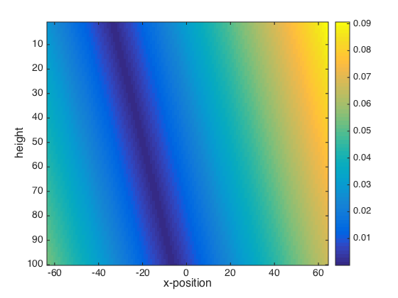
(a)

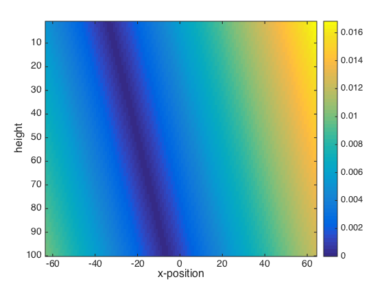
(b)

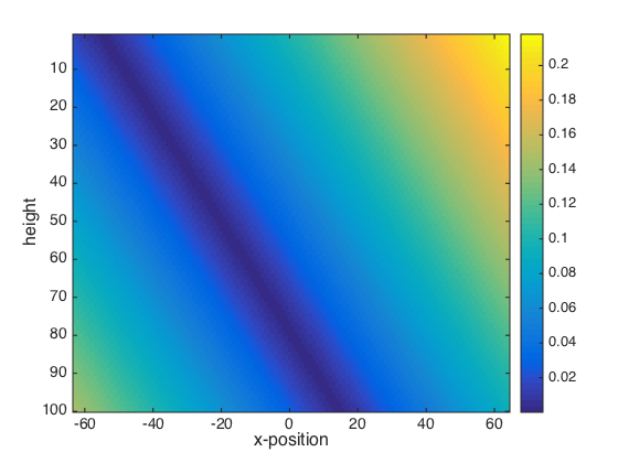
(c)

Figure 16: (a) Image of the magnitude of $\widehat{(\mathbf{z}-\bm{\gamma}_{1}(s_{d}^{1}))}\cdot\dot{\bm{\gamma}}_{1}(s_{d}^{1})-\frac{c}{\omega_{0}}f_{1}^{d}(\mathbf{x},s_{d}^{1})$ at $y=-31$m. The iso-Doppler contour is indicated by dark blue area where the magnitude of $\widehat{(\mathbf{z}-\bm{\gamma}_{1}(s_{d}^{1}))}\cdot\dot{\bm{\gamma}}_{1}(s_{d}^{1})=\frac{c}{\omega_{0}}f_{1}^{d}(\mathbf{x},s_{d}^{1})$ is minimized. (b) Image of the magnitude of $\widehat{(\mathbf{z}-\bm{\gamma}_{1}(s_{d}^{1}))}\cdot\ddot{\bm{\gamma}}_{1}(s_{d}^{1})-\frac{\dot{\bm{\gamma}}_{1}(s_{d}^{1})\cdot\dot{\bm{\gamma}}_{1}^{\perp}(s_{d}^{1}T_{\phi})}{R_{1}(s_{d}^{1},\mathbf{z})}-\partial_{s}f_{1}^{d}(\mathbf{x},s_{d}^{1})$ at $y=-31$m. The iso-Doppler-rate contour is indicated by dark blue area where the magnitude of $\widehat{(\mathbf{z}-\bm{\gamma}_{1}(s_{d}^{1}))}\cdot\ddot{\bm{\gamma}}_{1}(s_{d}^{1})-\frac{\dot{\bm{\gamma}}_{1}(s_{d}^{1})\cdot\dot{\bm{\gamma}}_{1}^{\perp}(s_{d}^{1}T_{\phi})}{R_{1}(s_{d}^{1},\mathbf{z})}-\partial_{s}f_{1}^{d}(\mathbf{x},s_{d}^{1})$ is minimized. (c) Image of the magnitude of $\mathbf{L}_{1}(\mathbf{z},s_{d}^{1})\cdot\mathbf{v}+\frac{\mathbf{b}_{1}^{\perp}\cdot\dot{\bm{\gamma}}_{2}(s_{d}^{2})}{R_{1}(\mathbf{z},s_{d}^{1})}+\frac{c}{2s_{d}^{1}T_{\phi}\omega_{0}}\Phi^{UNB}_{s_{d}}(\mathbf{x})$ at $y=-31$m. The interferometric Doppler-rate contour is indicated by dark blue area where the magnitude of $\mathbf{L}_{1}(\mathbf{z},s_{d}^{1})\cdot\mathbf{v}+\frac{\mathbf{b}_{1}^{\perp}\cdot\dot{\bm{\gamma}}_{2}(s_{d}^{2})}{R_{1}(\mathbf{z},s_{d}^{1})}+\frac{c}{2s_{d}^{1}T_{\phi}\omega_{0}}\Phi^{UNB}_{s_{d}}(\mathbf{x})$ is minimized.

Fig. 17 combines Figs. 16a, 16b, and 16c. The intersection of the three contours is indicated by white ‘x’. The white ‘o’ shows the true target location.

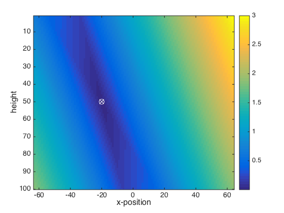
Figure 17: Image of the intersection of the iso-Doppler, iso-Doppler-rate and interferometric Doppler-rate contours at $y=-31$m. The intersection is indicated by white ‘x’. The true target position is indicated by white ‘o’. The target is reconstructed at the correct position and height.

Clearly, the target is reconstructed at the correct position and height.

7 Conclusions

We present a novel radar interferometry based on Doppler-SAR imaging paradigm. Doppler-SAR uses single frequency transmitted waveforms. It has several advantages over conventional SAR including simpler, inexpensive hardware, high SNR and long effective range of operation, and is suitable for use in passive radar applications.

We derived the interferometric phase relationship for Doppler-SAR. Doppler-SAR interferometric phase depends on the difference in the velocity of the antennas as opposed to the range difference observed in wideband SAR. Thus, in Doppler-SAR interferometry, one can reconstruct the ground topography even with the same look-direction from both antennas so long as their velocities are different). Furthermore, we showed that the true target position is determined by the intersection of iso-Doppler, iso-Doppler-rate, and interferometric Doppler-rate surfaces. This is different from conventional wideband SAR in that the surfaces that determine the true target position are iso-range, iso-Doppler, and interferometric Doppler-rate surfaces.

We presented numerical simulations for a single point scatterer using two antennas moving in linear trajectories to verify our interferometric method. We also conduct conventional wideband SAR interferometric reconstruction as a comparison. We show that both wideband SAR and Doppler-SAR interferometry is able to accurately reconstruct the target location. Thus, our numerical simulations show that Doppler-SAR interferometry retains the accuracy of conventional SAR interferometry while having the advantage that Doppler-SAR affords.

In the future, we will analyze the sensitivity of height estimation with respect to other observables and parameters.

Appendix A Approximations

A.1 Far-field approximation

Let $\brmn x$ and $\brmn y$ be two vectors such that $|\brmn x|\gg|\brmn y|$. Then, by using Taylor series expansion we can make the following approximation:

$$|\brmn x-\brmn y| = \sqrt{(x_{1}-y_{1})^{2}+(x_{2}-y_{2})^{2}+(x_{3}-y_{3})^{2}},$$ (61)

$$= \sqrt{|\brmn x|^{2}-2(x_{1}y_{1}+x_{2}y_{2}+x_{3}y_{3})+|\brmn y|^{2}},$$ (62)

$$= |\brmn x|\sqrt{1-\frac{2(\brmn x\cdot\brmn y)}{|\brmn x|^{2}}+\frac{|\brmn y|^{2}}{|\brmn x|^{2}}},$$ (63)

$$\approx |\brmn x|\left(1-\frac{1}{2}\frac{2\brmn x\cdot\brmn y}{|\brmn x|}\right),$$ (64)

$$\approx |\brmn x|-\hat{\brmn x}\cdot\brmn y$$ (65)

where $\hat{\brmn x}$ is the unit vector $\hat{\brmn x}=\frac{\brmn x}{|\brmn x|}$.

A.2 Approximation of look-direction under far-field assumption

Let $\widehat{(\brmn x-\bm{\gamma}(s))}$ denote a look direction where $\brmn x=\brmn y+\brmn z$ and $|\brmn y-\bm{\gamma}(s)|\gg|\brmn z|$. Then by using far field expansion we can write

$$\qquad\widehat{(\brmn x-\bm{\gamma}(s))} = \frac{\brmn x-\bm{\gamma}(s)}{|\brmn x-\bm{\gamma}(s)|}$$ (66)

$$= \frac{\brmn y+\brmn z-\bm{\gamma}(s)}{|\brmn y+\brmn z-\bm{\gamma}(s)|},$$ (67)

$$\approx \frac{\brmn y-\bm{\gamma}(s)}{|\brmn y-\bm{\gamma}(s)|+\widehat{(\brmn y-\bm{\gamma}(s))}\cdot\brmn z}+\frac{\brmn z}{|\brmn y-\bm{\gamma}(s)|+\widehat{(\brmn y-\bm{\gamma}(s))}\cdot\brmn z},$$ (68)

$$\approx (|\brmn y-\bm{\gamma}(s)|-\widehat{(\brmn y-\bm{\gamma}(s))}\cdot\brmn z)\frac{\brmn y-\bm{\gamma}(s)}{|\brmn y-\bm{\gamma}(s)|^{2}}$$ (70)

$$\qquad\qquad\ +\frac{(|\brmn y-\bm{\gamma}(s)|-\widehat{(\brmn y-\bm{\gamma}(s))}\cdot\brmn z)\brmn z}{|\brmn y-\bm{\gamma}(s)|^{2}},$$

$$\approx \widehat{(\brmn y-\bm{\gamma}(s))}+\frac{\brmn z-\widehat{(\brmn y-\bm{\gamma}(s))}\left[\widehat{(\brmn y-\bm{\gamma}(s))}\cdot\brmn z\right]}{|\brmn y-\bm{\gamma}(s)|},$$ (71)

$$\approx \widehat{(\brmn y-\bm{\gamma}(s))}+\frac{\brmn z^{\perp}}{|\brmn y-\bm{\gamma}(s)|}$$ (72)

where $\brmn z^{\perp}$ is the transverse $\brmn z$, i.e. projection of $\brmn z$ onto the plane whose normal vector is along the look direction $\widehat{(\bm{\gamma}(s)-\brmn y)}$. Therefore, difference of look directions is given by:

$$\widehat{(\brmn x-\bm{\gamma}(s))}-\widehat{(\brmn y-\bm{\gamma}(s))}\approx\frac{\brmn z^{\perp}}{|\bm{\gamma}(s)-\brmn y|}$$ (73)

where $\brmn x=\brmn y+\brmn z$.

References

References

- [1] Bamler R and Hartl P 1998 Inverse problems 14 R1
- [2] Rogers A and Ingalls R 1969 Science 165 797–799
- [3] Rogers A, Ingalls R and Rainville L 1972 The Astronomical Journal 77 100
- [4] Graham L C 1974 Proceedings of the IEEE 62 763–768
- [5] Zebker H A and Goldstein R M 1986 Journal of Geophysical Research: Solid Earth 91 4993–4999
- [6] Goldstein R M and Zebker H A 1987 Nature 328 707–709
- [7] Gabriel A K and Goldstein R M 1988 International Journal of Remote Sensing 9 857–872
- [8] Gabriel A K, Goldstein R M and Zebker H A 1989 Journal of Geophysical Research: Solid Earth 94 9183–9191
- [9] Hanssen R F 2001 Radar interferometry: data interpretation and error analysis vol 2 (Springer)
- [10] Rosen P A, Hensley S, Joughin I R, Li F K, Madsen S N, Rodriguez E and Goldstein R M 2000 Proceedings of the IEEE 88 333–382
- [11] Cherniakov M and Moccia A 2008 Bistatic radar: emerging technology (John Wiley & Sons) ISBN 9780470026311 URL http://books.google.com/books?id=a6nMEY2bKp4C
- [12] Fritz T, Rossi C, Yague-Martinez N, Rodriguez-Gonzalez F, Lachaise M and Breit H 2011 Interferometric processing of tandem-x data IEEE International Geoscience and Remote Sensing Symposium (IGARSS) (IEEE) pp 2428–2431
- [13] Duque S, Lopez-Dekker P and Mallorqui J 2010 Geoscience and Remote Sensing, IEEE Transactions on 48 2740–2749
- [14] Wang L and Yazici B 2012 IEEE Trans. Image Process. 21 3673–3686
- [15] Wang L and Yazici B 2013 Geoscience and Remote Sensing, IEEE Transactions on 51 4893–4910 ISSN 0196-2892
- [16] Wang L and Yazici B 2014 SIAM Journal on Imaging Sciences 7 824–866
- [17] Wang L and Yazici B 2012 Synthetic aperture radar imaging of moving targets using ultra-narrowband continuous waveforms 9th European Conf. Synthetic Aperture Radar (Nuremberg, Germany) pp 324–327
- [18] Wang L and Yazici B 2012 Detection and imaging of multiple ground moving targets using ultra-narrowband continuous-wave SAR SPIE Defense, Security, and Sensing (Baltimore, MD) pp 83940H–83940H
- [19] Wang L and Yazici B 2011 Bistatic synthetic aperture radar imaging using ultranarrow-band continuous waveforms IEEE Radar Conf. (Kansas City, MO) pp 062–067 ISSN 1097-5659
- [20] Wang L and Yazici B 2011 Ultranarrow-band synthetic aperture radar imaging for arbitrary flight trajectories 17th Int. Conf. Digital Signal Process. (Corfu, Greece) pp 1–6
- [21] Yarman C E, Wang L and Yazici B 2010 Inverse Problems 26 065006
- [22] Wang L, Yarman C E and Yazici B 2011 IEEE Transactions on Geoscience and Remote Sensing 49 3521–3537
- [23] Borden B and Cheney M 2004 Inverse Problems 21 1
- [24] Wang L, Yarman C E and Yazici B 2013 Theory of passive synthetic aperture imaging Excursions in Harmonic Analysis, Volume 1 (Springer) pp 211–236
- [25] Zebker H and Rosen P 1994 On the derivation of coseismic displacement fields using differential radar interferometry: The landers earthquake Geoscience and Remote Sensing Symposium, 1994. IGARSS’94. Surface and Atmospheric Remote Sensing: Technologies, Data Analysis and Interpretation., International vol 1 (IEEE) pp 286–288
- [26] Madsen S N, Zebker H A and Martin J 1993 IEEE Transactions on Geoscience and Remote sensing 31 246–256
- [27] Prati C, Rocca F, Guarnieri A M and Damonti E 1990 IEEE Transactions on Geoscience and Remote Sensing 28 627–640
- [28] Rodriguez E and Martin J 1992 Theory and design of interferometric synthetic aperture radars IEE Proceedings F-Radar and Signal Processing vol 139 (IET) pp 147–159
- [29] Nolan C and Cheney M 2003 IEEE Transactions on Image Processing 12 1035–1043
- [30] Yarman C and Yazıcı B 2008 IEEE Transactions on Image Processing 17 2156–2173
- [31] Yarman C, Yazıcı B and Cheney M 2008 IEEE Transactions on Image Processing 17 84–93
- [32] Prati C and Rocca F 1990 International Journal of Remote Sensing 11 2215–2235
- [33] Raney R, Runge H, Bamler R, Cumming I and Wong F 1994 Geoscience and Remote Sensing, IEEE Transactions on 32 786–799
- [34] Yazici B, Cheney M and Evren Y C 2006 Synthetic aperture inversion in the presence of noise and clutter Inverse Problems vol 22 (IOP Publishing) pp 1705–1729
- [35] Wang L and Yazici B 2011 Doppler synthetic aperture radar imaging Society of Photo-Optical Instrumentation Engineers (SPIE) Conference Series vol 8051 p 12