Stochastic Sequential Neural Networks
with Structured Inference

Abstract

Unsupervised structure learning in high-dimensional time series data has attracted a lot of research interests. For example, segmenting and labelling high dimensional time series can be helpful in behavior understanding and medical diagnosis. Recent advances in generative sequential modeling have suggested to combine recurrent neural networks with state space models (e.g., Hidden Markov Models). This combination can model not only the long term dependency in sequential data, but also the uncertainty included in the hidden states. Inheriting these advantages of stochastic neural sequential models, we propose a structured and stochastic sequential neural network, which models both the long-term dependencies via recurrent neural networks and the uncertainty in the segmentation and labels via discrete random variables. For accurate and efficient inference, we present a bi-directional inference network by reparamterizing the categorical segmentation and labels with the recent proposed Gumbel-Softmax approximation and resort to the Stochastic Gradient Variational Bayes. We evaluate the proposed model in a number of tasks, including speech modeling, automatic segmentation and labeling in behavior understanding, and sequential multi-objects recognition. Experimental results have demonstrated that our proposed model can achieve significant improvement over the state-of-the-art methods.

Keywords: Recurrent neural networks, Hidden Semi-Markov models, Sequential data

1 Introduction

Unsupervised structure learning in high-dimensional sequential data is an important research problem in a number of applications, such as machine translation, speech recognition, computational biology, and computational physiology Sutskever et al. (2014); Dai et al. (2017b). For example, in medical diagnosis, learning the segment boundaries and labeling of complicated physical signals is very useful for doctors to understand the underlying behavior or activity types.

Models for sequential data analysis such as recurrent neural networks (RNNs)Rumelhart et al. (1988) and hidden Markov models (HMMs)Rabiner (1989) are widely used. Recent literature have investigated approaches of combining probabilistic generative models and recurrent neural networks for the sake of their complementary strengths in nonlinear representation learning and effective estimation of parameters Johnson et al. (2016); Dai et al. (2017b); Fraccaro et al. (2016). In many tasks, such as segmentation and labeling of natural scenes and physiological signals, the duration lengths and labels of segments are often interpretable and categorical distributed  Jang et al. (2017). However, most of existing models are designed primarily for continuous situations and do not extend to discrete latent variables  Johnson et al. (2016); Krishnan et al. (2015); Archer et al. (2015); Krishnan et al. (2016), probably due to the difficulty of inference for discrete variables in neural networks. For example, the work in Krishnan et al. (2015) considers combining variational autoencoders Kingma and Welling (2013) with continuous state-space models, aiming to capture nonlinear dynamics with control inputs and leading to an RNN-based variational framework. The work in Johnson et al. (2016) proposes a state space model with a general emission density. When composed with neural networks, state space models are natural to model discrete variables. While discrete variables can be more interpretable and helpful in many applications like medical analysis and behavior prediction, they are less considered as switching variables in previous work  Fox et al. (2011); Johnson et al. (2016). Although the work in  Dai et al. (2017b) utilizes discrete variables with informative information for label prediction of segmentation, the inference approach does not explicitly take advantage of structured information to exploit the bi-directional temporal information, and thus may lead to suboptimal performance, as verified in the experiment (See Table 3 in Section 5 for more details).

To address such issues, we propose the Stochastic Sequential Neural Network (SSNN) consisting of a generative network and an inference network. The generative network(as will shown in Figure 2(a)) shares the spirit of Hidden Semi-Markov Model (HSMM) Rabiner (1989) and Recurrent HSMM Dai et al. (2017b), and is composed with a continuous sequence (i.e., hidden states in RNN) as well as two discrete sequences (i.e., segmentation variables and labels in SSM). The inference network(as will shown in Figure 2(b)) can take the advantages of bi-directional temporal information by augmented variables, and efficiently approximate the categorical variables in segmentation and segment labels via the recently proposed Gumbel-Softmax approximation Jang et al. (2017); Maddison et al. (2016). Thus, SSNN can model the complex and long-range dependencies in sequential data, but also maintain the structure learning ability of SSMs with efficient inference.

In order to evaluate the performance of the proposed model, we compare our proposed model with the state-of-the-art neural models in a number of tasks, including automatic segmentation and labeling on datasets of speech modeling, and behavior modeling, medical diagnosis, and multi-object recognition. Experimental results in terms of both model fitting and labeling of learned segments have demonstrated the promising performance of the proposed model.

2 Preliminaries

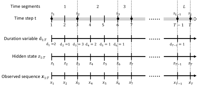
Figure 1: A visualization of the observed sequence $\mathbf{x}_{1:T}$ with the corresponding time segments, hidden states $z_{1:T}$ and duration variables $d_{1:T}$. In HMM, there is no duration variable $d_{t}$ and segments are pre-determined.

In this section, we present background related to generative sequential models. Specifically, we first introduce RNNs, followed by HMMs and HSMMs.

Recurrent neural networks (RNNs), as a wide range of sequential models for time series, have been applied in a number of applications Sutskever et al. (2014). Here we introduce basic properties and notations of RNNs. Consider a sequence of temporal sequences of vectors $\mathbf{x}_{1:T}=[\mathbf{x}_{1},\mathbf{x}_{2},...,\mathbf{x}_{T}]$ that depends on the inputs $\mathbf{u}_{1:T}=[\mathbf{u}_{1},\mathbf{u}_{2},...,\mathbf{u}_{T}]$, where $\mathbf{x}_{t}\in\mathbb{R}^{m}$ is the observation and $\mathbf{u}_{t}\in\mathbb{R}^{n}$ is the input at the time step $t$, and $T$ is the maximum time steps. RNN further introduces hidden states $\mathbf{h}_{1:T}=[\mathbf{h}_{1},\mathbf{h}_{2},...,\mathbf{h}_{T}]$, where $\mathbf{h}_{t}\in\mathbb{R}^{h}$ encodes the information before the time step $t$, and is determined by $\mathbf{h}_{t}=f_{\theta}(\mathbf{h}_{t-1},\mathbf{u}_{t})$, where $f_{\theta}(\cdot)$ is a nonlinear function parameterized by a neural network.

State space models such as hidden Markov models (HMMs) and hidden Semi-Markov models (HSMMs) are also widely-used methods in sequential learning Dai et al. (2017b); Chiappa et al. (2014); Dewar et al. (2012). In HMM, given an observed sequence $\mathbf{x}_{1:T}$, each $\mathbf{x}_{t}$ is generated based on the hidden state $z_{t}\in\{1,2,...,K\}$, and $p_{\theta}(\mathbf{x}_{t}|z_{t})$ is the emission probability. We set $p_{\theta}(z_{1})$ as the distribution of the initial state, and $p_{\theta}(z_{t}|z_{t-1})$ is the transition probability. We use $z_{1:T}=[z_{1},z_{2},...,z_{T}]$. Here $\theta$ includes all parameters necessary for these distributions. HSMM is a famous extension of HMM. Aside from the hidden state $z_{t}$, HSMM further introduces time duration variables $d_{t}\in\{1,2,..,M\}$, where $M$ is the maximum duration value for each $\mathbf{x}_{t}$. We set $d_{1:T}=[d_{1},d_{2},...,d_{T}]$. HSMM splits the sequence into $L$ segments, allowing the flexibility to find the best segment representation. We set $\mathbf{s}_{1:L}=[s_{1},s_{2},..,s_{L}]$ as the beginning of the segments. A difference from HMM is that for segment $i$, the latent state $z_{s_{i}:s_{i}+d_{s_{i}}-1}$ is fixed in HMM. An illustration is given in Figure 1.

There are many variants of HSMMs such as the Hierarchical Dirichlet-Process HSMM (HDP-HSMM) Johnson and Willsky (2013) and subHSMM Johnson and Willsky (2014). The subHSMM and HDP-HSMM extend their HMM counterparts by allowing explicit modeling of state duration lengths with arbitrary distributions. While there are various types of HMM, the inference methods are mostly inefficient.

Although HMMs and HSMMs can explicitly model uncertainty in the latent space and learn a interpretable representation through $d_{t}$ and $z_{t}$, they are not good at capturing the long-range temporal dependencies when compared with RNNs.

3 Model

In this section, we present our stochastic sequential neural network model. The notations and settings are generally consistent with HSMM Section 2, as also illustrated in Figure 1. For the simplicity of explanation, we present our model on a single sequence. It is straightforward to apply the model multiple sequences.

3.1 Generative Model

In order to model the long-range temporal dependencies and the uncertainty in segmentation and labeling of time series, we aim to take advantages from RNN and HSMM, and learn categorical information and representation information from the observed data recurrently. As illustrated in Figure 2(a), we design an Stochastic Sequential Neural Network (SSNN) with one sequence of continuous latent variables modeling the recurrent hidden states, and two sequences of discrete variables denoting the segment duration and labels, respectively. The joint probability can be factorized as:

$$p_{\theta}(\mathbf{x}_{1:T},z_{1:T},d_{1:T})=p_{\theta}(\mathbf{x}_{1:T}|z_{1:T},d_{1:T})\cdot p_{\theta}(z_{1})p_{\theta}(d_{1}|z_{1})\prod_{t=2}^{T}p_{\theta}(z_{t}|z_{t-1},d_{t-1})p_{\theta}(d_{t}|z_{t},d_{t-1}).$$ (1)

To learn more interpretative latent labels, we follow the design in HSMM to set $z_{t}$ and $d_{t}$ as categorical random variables, The distribution of $z_{t}$ and $d_{t}$ is

$$p_{\theta}(z_{t}|z_{t-1},d_{t-1})=\left\{\begin{aligned} \mathbb{I}(z_{t}=z_{t-1})\hskip 8.61108pt\text{if}\hskip 4.30554ptd_{t-1}>1\\ p_{\theta}(z_{t}|z_{t-1})\hskip 21.52771pt\text{otherwise}\end{aligned}\hskip 15.0694pt,\right.$$ (2)

$$p_{\theta}(d_{t}|z_{t},d_{t-1})=\left\{\begin{aligned} \mathbb{I}(d_{t}=d_{t-1}-1)\hskip 8.61108pt\text{if}\hskip 4.30554ptd_{t-1}>1\\ p_{\theta}(d_{t}|z_{t})\hskip 47.36096pt\text{otherwise}\end{aligned}\hskip 8.61108pt,\right.$$ (3)

where $\mathbb{I}(x)$ is the indicator function (whose value equals $1$ if $x$ is True, and otherwise $0$). The transition probability $p_{\theta}(z_{t}|z_{t-1})$ and $p_{\theta}(d_{t}|z_{t})$, in implementation, can be achieved by learning a transition matrix.

The joint emission probability $p_{\theta}(\mathbf{x}_{1:T}|z_{1:T},d_{1:T})$ can be further factorized into multiple segments. Specifically, for the $i$-th segment $\mathbf{x}_{s_{i}:s_{i}+d_{s_{i}}-1}$ starting from $s_{i}$, the corresponding generative distribution is

$$p_{\theta}(\mathbf{x}_{s_{i}:s_{i}+d_{s_{i}}-1}|z_{s_{i}},d_{s_{i}})=\prod_{t=s_{i}}^{s_{i}+d_{s_{i}}-1}p_{\theta}(\mathbf{x}_{t}|\mathbf{x}_{s_{i}:t-1},z_{s_{i}}).=\prod_{t=s_{i}}^{s_{i}+d_{s_{i}}-1}p_{\theta}(\mathbf{x}_{t}|\mathbf{h}_{t},z_{s_{i}}),$$ (4)

where $\mathbf{h}_{t}$ is the latent deterministic variable in RNN. As mentioned earlier, $\mathbf{h}_{t}$ can better model the complex dependency among segments, and capture past information of the observed sequence $\mathbf{x}_{t-1}$ as well as the previous state $\mathbf{h}_{t-1}$. We design $\mathbf{h}_{t}=\sigma(\mathbf{W}_{x}^{(z_{s_{i}})}\mathbf{x}_{t-1}+\mathbf{W}_{h}^{(z_{s_{i}})}\mathbf{h}_{t-1}+\mathbf{b}_{h}^{(z_{s_{i}})})$, where $\sigma()$ is a tanh activation function, $\mathbf{W}_{x}\in\mathbb{R}^{K\times h\times m}$ and $\mathbf{W}_{h}\in\mathbb{R}^{K\times h\times h}$ are weight parameter, and $\mathbf{b}_{h}\in\mathbb{R}^{K\times h}$ is the bias term. $\mathbf{W}_{x}^{(z_{s_{i}})}\in\mathbb{R}^{h\times m}$ is the $z_{s_{i}}$-th slice of $\mathbf{W}_{x}$, and it is similar for $\mathbf{W}_{h}^{(z_{s_{i}})}$ and $\mathbf{b}_{h}^{(z_{s_{i}})}$.

Finally, the distribution of $\mathbf{x}_{t}$ given $\mathbf{h}_{t}$ and $z_{s_{i}}$ is designed by a Normal distribution,

$$p_{\theta}(\mathbf{x}_{t}|\mathbf{h}_{t},z_{s_{i}})=\mathcal{N}(x;\bm{\mu},\bm{\sigma}^{2}),$$ (5)

where the mean satisfies $\bm{\mu}=\mathbf{W}_{\mu}^{(z_{s_{i}})}\mathbf{h}_{t}+b_{\mu}^{(z_{s_{i}})}$, and the covariance is a diagonal matrix with its log diagonal elements $\log\bm{\sigma}^{2}=\mathbf{W}_{\sigma}^{(z_{s_{i}})}\mathbf{h}_{t}+\mathbf{b}_{\sigma}^{(z_{s_{i}})}$. We use $\theta$ to include all the parameters in the generative model.

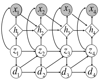
(a) Generative network

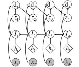
(b) Inference network

Figure 2: The generative network and inference network of SSNN. The generative network can be viewed as a HSMM with recurrent structure on hidden states. The inference network is designed by backwards recurrent function through $\mathcal{I}_{t}$ for each segment. Diamond units are deterministic variables, while circles are random variables.

3.2 Structured Inference

We are interested in maximizing the marginal log-likelihood $\log p(\mathbf{x})$, however, this is usually intractable since the complicated posterior distributions cannot be integrated out generally. Recent methods in Bayesian learning, such as the score function (or REINFORCE) Archer et al. (2015) and the Stochastic Gradient Variational Bayes (SGVB) Kingma and Welling (2013), are common black-box methods that lead to tractable solutions. We resort to the SGVB since it could efficiently learn the approximation with relatively low variances Kingma and Welling (2013), while the score function suffers from high variances and heavy computational costs.

We now focus on maximizing the evidence lower bound also known as $ELBO$,

$$\log p_{\theta}(\mathbf{x})\geq\mathcal{L}(\mathbf{x}_{1:T};\theta,\phi)=E_{q_{\phi}(z_{1:T},d_{1:T}|\mathbf{x}_{1:T})}[\log p_{\theta}(\mathbf{x}_{1:T},z_{1:T},d_{1:T})-\log q_{\phi}(z_{1:T},d_{1:T}|\mathbf{x}_{1:T})],$$ (6)

where $q_{\phi}(\cdot)$ denotes the approximate posterior distribution, and $\theta$ and $\phi$ denote parameters for their corresponding distributions, repsectively.

3.2.1 Bi-directional Inference

In order to find a more informative approximation to the posterior, we augment both random variables $d_{t}$, $z_{t}$ with bi-directional information in the inference network. Such attempts have been explored in many previous work (Krishnan et al., 2016; Khan and Lin, 2017; Krishnan et al., 2015), however they mainly focus on continuous variables, and little attention is paid to the discrete variable. Specifically, we first learn a bi-directional deterministic variable $\hat{\mathbf{h}_{t}}=\text{BiRNN}(x_{1:t},x_{t:T})$ , where BiRNN is a bi-directional RNN with each unit implemented as an LSTM Hochreiter and Schmidhuber (1997). Similar to Fraccaro et al. (2016), we further use a backward recurrent function $I_{t}=g_{\phi_{I}}(I_{t+1},[\mathbf{x}_{t},\hat{\mathbf{h}_{t}}])$ to explicitly capture forward and backward information in the sequence via $\hat{\mathbf{h}_{t}}$, where $[\mathbf{x}_{t},\hat{\mathbf{h}_{t}}]$ is the concatenation of $\mathbf{x}_{t}$ and $\hat{\mathbf{h}_{t}}$.

The posterior approximation can be factorized as

$$q_{\phi}(z_{1:T},d_{1:T}|\mathbf{x}_{1:T})=q_{\phi}(z_{1}|I_{1})q_{\phi}(d_{1}|z_{1},I_{1})\prod_{t=2}^{T}q_{\phi}(z_{t}|d_{t-1},I_{t})q_{\phi}(d_{t}|d_{t-1},z_{t},I_{t}),$$ (7)

and the graphical model for the inference network is shown in Figure.2(b). We use $\phi$ to denotes all parameters in inference network.

We design the posterior distributions of $d_{t}$ and $z_{t}$ to be categorical distributions, respectively, as follows:

$$q(z_{t}|d_{t-1},I_{t};\phi)=\mathrm{Cat}(\text{softmax}(\mathbf{W}_{z}^{T}I_{t})),$$ (8)

$$q(d_{t}|d_{t-1},z_{t},I_{t};\phi)=\mathrm{Cat}(\text{softmax}(\mathbf{W}_{d}^{T}I_{t})),$$ (9)

where $\mathrm{Cat}$ denotes the categorical distribution. Since the posterior distributions of $z_{t}$ and $d_{t}$ are conditioned on $I_{t}$, they depend on both the forward sequences (i.e., $h_{t:T}$ and $x_{t:T}$) and the backward sequences (i.e., $h_{1:t-1}$ and $x_{1:t-1}$), leading to a more informative approximation. However, the reparameterization tricks and their extensions (Chung et al., 2016) are not directly applicable due to the discrete random variables, i.e., $d_{t}$ and $z_{t}$ in our model. Thus we turn to the recently proposed Gumbel-Softmax reparameterization trick (Jang et al., 2017; Maddison et al., 2016), as shown in the following.

3.2.2 Gumbel-Softmax Reparameterization

The Gumbel-Softmax reparameterization proposes an alternative to the back propagation through discrete random variables via the Gumbel-Softmax distribution, and circumvents the non-differentiable categorical distribution.

To use the Gumbel-Softmax reparameterization, we first map the discrete pair $(z_{t},d_{t})$ to a $N$-dimensional vector $\bm{\gamma}(t)$, and $\bm{\gamma}(t)\sim\mathrm{Cat}(\bm{\pi}(t))$, where $\bm{\pi}(t)$ is a $N$-dimensional vector on the simplex and $N=K\times D$. Then we use $\mathbf{y}(t)\in\mathbb{R}^{N}$ to represent the Gumbel-Softmax distributed variable:

$$y_{i}(t)=\frac{\text{exp}((\log(\pi_{i}(t))+g_{i})/\tau)}{\sum_{j=1}^{k}\text{exp}((\log(\pi_{j}(t))+g_{j})/\tau)}\qquad\text{for }i=1,...,N,$$ (10)

where $g_{i}\sim\mathrm{Gumbel}(0,1)$, and $\tau$ is the temperature that will be elaborated in the experiment. Via the Gumbel Softmax transformation, we set $\mathbf{y}(t)\sim\textrm{Concrete}(\bm{\pi}(t),\tau)$ according to (Maddison et al., 2016).

Now we can sample $\mathbf{y}(t)$ from the Gumbel-Softmax posterior in replacement of the categorically distributed $\bm{\gamma}(t)$, and use the back-propagation gradient with the ADAM Kingma and Ba (2014) optimizer to learn parameters $\theta$ and $\phi$.

For simplicity, we denote $F(z,d)=\log p_{\theta}(\mathbf{x}_{1:T},z_{1:T},d_{1:T})-\log q(z_{1:T},d_{1:T}|\mathbf{x}_{1:T})$, and furthermore, $\tilde{F}(y,g)$ is the corresponding approximation term of $F(z,d)$ after the Gumbel-Softmax trick. The Gumbel-Softmax approximation of $\mathcal{L}(\mathbf{x}_{1:T};\theta,\phi)$ is:

$$\mathcal{L}(\mathbf{x}_{1:T};\theta,\phi)\approx E_{y\sim\mathrm{Concrete}(\bm{\pi}(t),\tau)}[\tilde{F}(y,g)]=E_{g\sim\prod_{N}\mathrm{Gumbel}(0,1)}[\tilde{F}(y,g)].$$ (11)

Hence the derivatives of the approximated $ELBO$ w.r.t. the inference parameters $\phi$ can be approximated by the SGVB estimator:

$$\frac{\partial}{\partial\phi}E_{g\sim\prod_{N}\mathrm{Gumbel}(0,1)}[\tilde{F}(y,g)] =E_{g\sim\prod_{N}\mathrm{Gumbel}(0,1)}\left[\frac{\partial}{\partial\phi}\left(\tilde{F}(y,g)\right)\right]$$

$$\approx\frac{1}{B}\sum_{b=1}^{B}\frac{\partial}{\partial\phi}\left(\tilde{F}(y^{b},g^{b})\right),\hskip 8.61108ptg^{b}:=(g_{1}^{b},\dotsc,g_{N}^{b}),$$ (12)

where $y^{b},g^{b}$ is the batch samples and $B$ is the number of batches. The derivative w.r.t the generative parameters $\theta$ does not require the Gumbel-Softmax approximation, and can be directly estimated by the Monte Carlo estimator

$$\frac{\partial}{\partial\theta}E_{q_{\phi}(z_{1:T},d_{1:T})}[F(z,d)]\approx\frac{1}{B}\sum_{b=1}^{B}\frac{\partial}{\partial\theta}\left(F(z^{b},d^{b})\right).\hskip 8.61108pt$$ (13)

Finally, we summarize the inference algorithm in Algorithm 1.

Algorithm 1 Strucutured Inference Algorithm for SSNN

  inputs: Observed sequences $\{\mathbf{x}^{(n)}\}_{n=1}^{N}$

       Randomly initialized $\phi^{(0)}$ and $\theta^{(0)}$;

       Inference Model: $q_{\phi}(z_{1:T},d_{1:T}|\mathbf{x}_{1:T})$;

       Generative Model: $p_{\theta}(\mathbf{x}_{1:T},z_{1:T},d_{1:T})$;

  outputs:Model parameters $\theta$ and $\phi$;

  for $i=1$ to $Iter$ do

     1. Sample sequences $\{x^{(n)}\}_{n=1}^{M}$ uniformly from dataset with a mini-batch size $B$.

     2. Estimate and sample forward parameters using Eq.(1).

     3. Evaluate the ELBO using Eq. (6).

     4. Estimate the Monte Carlo approximation to $\nabla_{\theta}L$ using Eq. (13)

     5. Estimate the SGVB approximation to $\nabla_{\phi}L$ using Eq.(3.2.2) with the Gumbel-Softmax approximation in Eq.(10);

     6. Update $\theta^{(i)}$, $\phi^{(i)}$ using the ADAM.

  end for

4 Related Work

In this section, we review research work on generative sequential data modeling in terms of state space models and recurrent neural networks. In the following, we review some recent work on sequential latent variable model.

In terms of combining both and SSM and RNNs, the papers mostly close to our paper include Johnson et al. (2016); Krishnan et al. (2015, 2016); Archer et al. (2015); Fraccaro et al. (2016). In detail, Krishnan et al. (2015) combines variational auto-encoders with continuous state-space models, emphasizing the relationship to linear dynamical systems. Krishnan et al. (2016) lets inference network conditioned on both future and past hidden variables, which extends Deep Kalman Filtering. Archer et al. (2015) uses a structured Gaussian variational family to solve the problem of variational inference in general continuous state space models without considering parameter learning. And Johnson et al. (2016) can employ general emission density for structured inference. Fraccaro et al. (2016) extends state space models by combining recurrent neural networks with stochastic latent variables. Different from the above methods that require the hidden states of SSM be continuous, our paper utilizes discrete latent variables in the SSM part for better interpretablity, especially in applications of segmentation and labeling of high-dimensional time series.

In parallel, some research also works on variational inference with discrete latent variables recently. Bayer and Osendorfer (2014) enhances recurrent neural networks with stochastic latent variables which they call stochastic neural network. For stochastic neural network the most applicable approach is the score function or REINFORCE approach, however it suffers from high variance. Mnih and Rezende (2016) proposes a gradient estimator for multi-sample objectives that use the mean of other samples to construct a baseline for each sample to decrease variance. Gu et al. (2015b) also models the baseline as a first-order Taylor expansion and overcomes back propagation through discrete sampling with a mean-field approximation, so it becomes practical to compute the baseline and derive the relevant gradients. Gregor et al. (2013) uses the first-order Taylor approximation as a baseline to reduce variances. In Discrete VAE Rolfe (2016), the sampling is autoregressive through each binary unit, which allows every discrete choice to be marginalized out in a tractable manner. Dai et al. (2017b) proposes to overcome the difficulty of learning discrete variables by optimizing their distribution instead of directly learning discrete variables.

In the aspect of optimization, Khan et al. (2015a, b) split the variational inference objective into a term to be linearized and a tractable concave term, which makes the resulting gradient easily to compute. Knowles and Minka (2011) proposes natural gradient descent with respect to natural parameters on each of the variational factors in turn. In Dai et al. (2017a), the discrete optimization is replaced by the maximization over the negative Helmholtz free energy. In contrast to linearizing intractable terms around the current iteration as used in the above approaches, we handle intractable terms via recognition networks and amortized inference(with the aid of Gumbel-Softmax reparameterization Jang et al. (2017); Maddison et al. (2016)) in this paper. That is, we use parametric function approximators to learn conditional evidence in a conjugate form.

5 Experiment

In this section, we evaluate SSNN on several datasets across multiple scenarios. Specifically, we first evaluate its performance of finding complex structures and estimating data likelihood on a synthetic dataset and two speech datasets (TIMIT & Blizard). Then we test SSNN with learning segmentations and latent labels on Human activity Reyes-Ortiz et al. (2016) dataset, Drosophila dataset Kain et al. (2013) and PhysioNet Springer et al. (2016) Challenge dataset, and compare the results with HSMM and its variants. Finally we provide an additional challenging test on the multi-object recognition problem using the generated multi-MNIST dataset.

All models in the experiment use the Adam Kingma and Ba (2014) optimizer. Temperatures of Gumbel-Softmax were fixed throughout training. We implement the proposed model based on Theano Al-Rfou et al. (2016) and Block & Fuel Van Merriënboer et al. (2015).

5.1 Synthetic Experiment

To validate that our method is able to model high dimensional data with complex dependency, we simulated a complex dynamic torque-controlled pendulum governed by a differential equation to generate non-Markovian observations from a dynamical system: $ml^{2}\frac{d^{2}\phi(t)}{dt^{2}}=-\mu\frac{d\phi(t)}{dt}+mgl\sin\phi(t)+u(t)$. For fair comparison with Karl et al. (2016), we set $m=l=1$, $\mu=0.5$, and $g=9.81$. We convert the generated ground-truth angles to image observations. The system can be fully described by angle and angular velocity.

We compare our method with Deep Variational Bayes Filter(DVBF-LL) Karl et al. (2016) and Deep Kalman Filters(DKF) Krishnan et al. (2015). The ordinary least square regression results are shown in Table  1. Our method is clearly better than DVBF-LL and DKF in predicting $\sin\phi$, $\cos\phi$ and $\frac{d\phi}{dt}$. SSNN achieves a higher goodness-of-fit than other methods. The results indicate that generative model and inference network in SSNN are capable of capturing complex sequence dependency.

		DVBF-LL		DKF		Our method (SSNN)
		log-likelihood	$R^{2}$	log-likelihood	$R^{2}$	log-likelihood	$R^{2}$
Measured	$\sin\phi$	3990.8	0.961	1737.6	0.929	4424.6	0.975
groundtruth	$\cos\phi$	7231.1	0.982	6614.2	0.979	8125.3	0.997
variables	$\frac{d\phi}{dt}$	-11139	0.916	-20289	0.035	-9620	0.941

Table 1: The results measured on the log-likelihood and the goodness-of-fit (denoted by $R^{2}$) given by three methods on the prediction of all latent states on respective dependent variables in pendulum dynamics. For both measures, the higher the better.

5.2 Speech Modeling

We also test SSNN on the modeling of speech data, i.e., Blizzard and TIMIT datasets Prahallad et al. (2013). Blizzard records the English speech with 300 hours by a female speaker. TIMIT is a dataset with 6300 English sentences read by 630 speakers. For the TIMIT and Blizzard dataset, the sampling frequency is 16KHz and the raw audio signal is normalized using the global mean and standard deviation of the training set. Speech modeling on these two datasets has shown to be challenging since there’s no good representation of the latent states Chung et al. (2015); Fabius and van Amersfoort (2014); Gu et al. (2015a); Gan et al. (2015); Sutskever et al. (2014).

The data preprocessing and the performance measures are identical to those reported in Chung et al. (2015); Fraccaro et al. (2016), i.e. we report the average log-likelihood for half-second sequences on Blizzard, and report the average log-likelihood per sequence for the test set sequences on TIMIT. For the raw audio datasets, we use a fully factorized Gaussian output distribution.

In the experiment, We split the raw audio signals in the chunks of 2 seconds. The waveforms are divided into non-overlapping vectors with size 200. For Blizzard we split the data using 90$\%$ for training, 5$\%$ for validation and 5$\%$ for testing. For testing we report the average log-likelihood for each sequence with segment length 0.5s. For TIMIT we use the predefined test set for testing and split the rest of the data into 95$\%$ for training and 5$\%$ for validation.

During training we use back-propagation through time (BPTT) for 1 second. For the first second we initialize hidden units with zeros and for the subsequent 3 chunks we use the previous hidden states as initialization. the temperature $\tau$ starts from a large value 0.1 and gradually anneals to 0.01.

We compare our method with the following methods. For RNN+VRNNs Chung et al. (2015), VRNN is tested with two different output distributions: a Gaussian distribution (VRNN-GAUSS), and a Gaussian Mixture Model (VRNN-GMM). We also compare to VRNN-I in which the latent variables in VRNN are constrained to be independent across time steps. For SRNN Fraccaro et al. (2016), we compare with the smoothing and filtering performance denoted as SRRR (smooth), SRNN (filt) and SRNN (smooth+ $Res_{q}$) respectively. The results of VRNN-GMM, VRNN-Gauss and VRNN-I-Gauss are taken from Chung et al. (2015), and those of SRNN (smooth+$Res_{q}$), SRNN (smooth) and SRNN (filt) are taken from Fraccaro et al. (2016). From Table 5.3 it can be observed that on both datasets SSNN outperforms the state of the art methods by a large margin, indicating its superior ability in speech modeling.

5.3 Segmentation and Labeling of Time Series

To show the advantages of SSNN over HSMM and its variants when learning the segmentation and latent labels from sequences, we take experiments on Human activity Reyes-Ortiz et al. (2016), Drosophila dataset Kain et al. (2013) and PhysioNet Springer et al. (2016) Challenge dataset.Both Human Activity and Drosophila dataset are used for segmentation prediction.

Human activity consists of signals collected from waist-mounted smartphones with accelerometers and gyroscopes. Each volunteer is asked to perform 12 activities. There are 61 recorded sequences, and the maximum time steps $T\approx 3,000$. Each $\mathbf{x}_{t}$ is a 6 dimensional vector.

Drosophila dataset records the time series movement of fruit flies’ legs. At each time step $t$, $\mathbf{x}_{t}$ is a 45-dimension vector, which consists of the raw and some higher order features. the maximum time steps $T\approx 10,000$. In the experiment, we fix the $\tau$ at small value $0.0001$.

PhysioNet Challenge dataset records observation labeled with one of the four hidden states, i.e., Diastole, S1, Systole and S2. The experiment aims to exam SSNN on learning and predicting the labels. In the experiment, we find that annealing of temperature $\tau$ is important, we start from $\tau=0.15$ and anneal it gradually to $0.0001$.

Models	Blizzard	TIMIT
VRNN-GMM	$\geq$ 9107	$\geq$ 28982
VRNN-Gauss	$\geq$ 9223	$\geq$ 28805
VRNN-I-Gauss	$\geq$ 9223	$\geq$28805
SRNN(smooth+$Res_{q}$)	$\geq$ 11991	$\geq$ 60550
SRNN(smooth)	$\geq$10991	$\geq$59269
SRNN(filt)	$\geq$10846	50524
RNN-GMM	7413	26643
RNN-Gauss	3539	-1900
Our Method(SSNN)	$\geq$ 13123	$\geq$ 64017

Table 2: Average log-likelihood per sequence on the test sets. The higher the better.

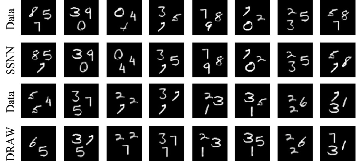
Figure 3: Visualization and comparison of SSNN and DRAW on multi-object recognition problems.

Models	Drosophila	Human activity	Physionet
HSMM	47.37 $\pm$ 0.27%	41.59 $\pm$ 8.58 %	45.04 $\pm$ 1.87 %
subHSMM	39.70 $\pm$ 2.21%	22.18 $\pm$ 4.45%	43.01 $\pm$ 2.35 %
HDP-HSMM	43.59 $\pm$ 1.58%	35.46 $\pm$ 6.19%	42.58 $\pm$ 1.54 %
CRF-AE	57.62 $\pm$ 0.22%	49.26 $\pm$ 10.63%	45.73 $\pm$ 0.66 %
rHSMM-dp	36.21 $\pm$ 1.37%	16.38 $\pm$ 5.06%	31.95 $\pm$ 4.12 %
SSNN	34.77 $\pm$ 3.70%	14.70 $\pm$ 5.45%	29.29 $\pm$ 5.34 %

Table 3: Mean and standard deviation of the error rate. For the Drosophila and Human Activity datasets, we report the error rate of segmentation. On the PhysioNet dataset, we report the error rate of latent label prediction. The results of subHSMM, HDP-HSMM, CRF-AE and RHSMM-DP are taken from subHSMM Johnson and Willsky (2014), HDP-HSMM Johnson and Willsky (2013), CRF-AE Ammar et al. (2014) and rHSMM-dp Dai et al. (2017b).

Specifically, we compare the predicted segments or latent labels with the ground truth, and report the mean and the standard deviation of the error rate for all methods. We use leave-one-sequence-out protocol to evaluate these methods, i.e., each time one sequence is held out for testing and the left sequences are for training. We set the truncation of max possible duration $M$ to be 400 for all tasks. We also set the number of hidden states $K$ to be the same as the ground truth.

We report the comparison with subHSMM Johnson and Willsky (2014), HDP-HSMM Johnson and Willsky (2013), CRF-AE Ammar et al. (2014) and rHSMM-dp Dai et al. (2017b).

For the HDP-HSMM and subHSMM, the observed sequences $\mathbf{x}_{1:T}$ are generated by standard multivariate Gaussian distributions. The duration variable $d_{t}$ is from the Poisson distribution. We need to tune the concentration parameters $\alpha$ and $\gamma$. As for the hyper parameters, they can be learned automatically. For subHSMM, we tune the truncation threshold of the infinite HMM in the second level. For CRF-AE, we extend the original model to learn continuous data. We use mixture of Gaussian for the emission probability. For R-HSMM-dp, it is a version of R-HSMM with the exact MAP estimation via dynamic programming.

Experimental results are shown in Table 3. It can be observed that SSNN achieves the lowest mean error rate, indicating the effectiveness of combining RNN with HSMM to collectively learn the segmentation and the latent states.

5.4 Sequential Multi-objects Recognition

In order to further verify the ability of modeling complex spatial dependency, we test SSNN on the multiple objects recognition problem. This problem is interesting but hard, since it requires the model to capture the dependency of pixels in images and recognize the objects in images. Specifically, we construct a small image dataset including 3000 images, named as multi-MNIST. Each image contains three non-overlapping random MNIST digits with equal probability.

Our goal is to sequentially recognize each digit in the image. In the experiment, we train our model with 2500 images and test on the rest 500 images.First we fix the maximum time steps $T=3$ and feed the same image as input sequentially to SSNN. We interpret the latent variable $d_{t}$ as intensity and $z_{t}$ as the location variable in the training images. Then We train SSNN with random initialized parameters on 60,000 multi-MNIST images from scratch, i.e., without a curriculum or any form of supervision. All experiments were performed with a batch size of 64. The learning rate of model is $1\times 10^{-5}$ and baselines were trained using a higher learning rate $1\times 10^{-3}$. The LSTMs in the inference network had 256 cell units.

We compare the proposed model to DRAW Gregor et al. (2015) and visualize our learned latent representations in Figure 5.3. It can be observed that our model identifies the number and locations of digits correctly, while DRAW sometimes misses modes of data. The result shows that our method can accurately capture not only the number of objects but also locations.

6 Conclusion

In order to learn the structures (e.g., the segmentation and labeling) of high-dimensional time series in a unsupervised way, we have proposed a Stochastic sequential neural network(SSNN) with structured inference. For better model interpretation, we further restrict the label and segmentation duration to be two sequences of discrete variables, respectively. In order to exploit forward and backward temporal information, we carefully design structured inference, and to overcome the difficulties of inferring discrete latent variables in deep neural networks, we resort to the recently proposed Gumbel-Softmax functions. The advantages of the proposed inference method in SSNN have been demonstrated in both synthetic and real-world sequential benchmarks.

Acknowledgments

This paper was in part supported by Grants from the Natural Science Foundation of China (No. 61572111), the National High Technology Research and Development Program of China (863 Program) (No. 2015AA015408), a 985 Project of UESTC (No.A1098531023601041), and two Fundamental Research Funds for the Central Universities of China (Nos. ZYGX2016J078 and ZYGX2016Z003).

References

- Al-Rfou et al. (2016) Rami Al-Rfou, Guillaume Alain, Amjad Almahairi, Christof Angermueller, Dzmitry Bahdanau, Nicolas Ballas, Frédéric Bastien, Justin Bayer, Anatoly Belikov, Alexander Belopolsky, et al. Theano: A python framework for fast computation of mathematical expressions. arXiv preprint arXiv:1605.02688, 2016.
- Ammar et al. (2014) Waleed Ammar, Chris Dyer, and Noah A Smith. Conditional random field autoencoders for unsupervised structured prediction. In Advances in Neural Information Processing Systems, pages 3311–3319, 2014.
- Archer et al. (2015) Evan Archer, Il Memming Park, Lars Buesing, John Cunningham, and Liam Paninski. Black box variational inference for state space models. arXiv preprint arXiv:1511.07367, 2015.
- Bayer and Osendorfer (2014) Justin Bayer and Christian Osendorfer. Learning stochastic recurrent networks. arXiv preprint arXiv:1411.7610, 2014.
- Chiappa et al. (2014) Silvia Chiappa et al. Explicit-duration markov switching models. Foundations and Trends® in Machine Learning, 7(6):803–886, 2014.
- Chung et al. (2015) Junyoung Chung, Kyle Kastner, Laurent Dinh, Kratarth Goel, Aaron C Courville, and Yoshua Bengio. A recurrent latent variable model for sequential data. In Advances in neural information processing systems, pages 2980–2988, 2015.
- Chung et al. (2016) Junyoung Chung, Sungjin Ahn, and Yoshua Bengio. Hierarchical multiscale recurrent neural networks. arXiv preprint arXiv:1609.01704, 2016.
- Dai et al. (2017a) Bo Dai, Ruiqi Guo, Sanjiv Kumar, Niao He, and Le Song. Stochastic generative hashing. arXiv preprint arXiv:1701.02815, 2017a.
- Dai et al. (2017b) Hanjun Dai, Bo Dai, Yan-Ming Zhang, Shuang Li, and Le Song. Recurrent hidden semi-markov model. ICLR, 2017b.
- Dewar et al. (2012) Michael Dewar, Chris Wiggins, and Frank Wood. Inference in hidden markov models with explicit state duration distributions. IEEE Signal Processing Letters, 19(4):235–238, 2012.
- Fabius and van Amersfoort (2014) Otto Fabius and Joost R van Amersfoort. Variational recurrent auto-encoders. arXiv preprint arXiv:1412.6581, 2014.
- Fox et al. (2011) Emily Fox, Erik B Sudderth, Michael I Jordan, and Alan S Willsky. Bayesian nonparametric inference of switching dynamic linear models. IEEE Transactions on Signal Processing, 59(4):1569–1585, 2011.
- Fraccaro et al. (2016) Marco Fraccaro, Søren Kaae Sønderby, Ulrich Paquet, and Ole Winther. Sequential neural models with stochastic layers. In Advances in Neural Information Processing Systems, pages 2199–2207, 2016.
- Gan et al. (2015) Zhe Gan, Chunyuan Li, Ricardo Henao, David E Carlson, and Lawrence Carin. Deep temporal sigmoid belief networks for sequence modeling. In Advances in Neural Information Processing Systems, pages 2467–2475, 2015.
- Gregor et al. (2013) Karol Gregor, Ivo Danihelka, Andriy Mnih, Charles Blundell, and Daan Wierstra. Deep autoregressive networks. arXiv preprint arXiv:1310.8499, 2013.
- Gregor et al. (2015) Karol Gregor, Ivo Danihelka, Alex Graves, Danilo Jimenez Rezende, and Daan Wierstra. Draw: A recurrent neural network for image generation. arXiv preprint arXiv:1502.04623, 2015.
- Gu et al. (2015a) Shixiang Gu, Zoubin Ghahramani, and Richard E Turner. Neural adaptive sequential monte carlo. In Advances in Neural Information Processing Systems, pages 2629–2637, 2015a.
- Gu et al. (2015b) Shixiang Gu, Sergey Levine, Ilya Sutskever, and Andriy Mnih. Muprop: Unbiased backpropagation for stochastic neural networks. arXiv preprint arXiv:1511.05176, 2015b.
- Hochreiter and Schmidhuber (1997) Sepp Hochreiter and Jürgen Schmidhuber. Long short-term memory. Neural computation, 9(8):1735–1780, 1997.
- Jang et al. (2017) Eric Jang, Shixiang Gu, and Ben Poole. Categorical reparameterization with gumbel-softmax. stat, 1050:1, 2017.
- Johnson and Willsky (2014) Matthew Johnson and Alan Willsky. Stochastic variational inference for bayesian time series models. In International Conference on Machine Learning, pages 1854–1862, 2014.
- Johnson et al. (2016) Matthew Johnson, David K Duvenaud, Alex Wiltschko, Ryan P Adams, and Sandeep R Datta. Composing graphical models with neural networks for structured representations and fast inference. In Advances in Neural Information Processing Systems, pages 2946–2954, 2016.
- Johnson and Willsky (2013) Matthew J Johnson and Alan S Willsky. Bayesian nonparametric hidden semi-markov models. Journal of Machine Learning Research, 14(Feb):673–701, 2013.
- Kain et al. (2013) Jamey Kain, Chris Stokes, Quentin Gaudry, Xiangzhi Song, James Foley, Rachel Wilson, and Benjamin De Bivort. Leg-tracking and automated behavioural classification in drosophila. Nature communications, 4:1910, 2013.
- Karl et al. (2016) Maximilian Karl, Maximilian Soelch, Justin Bayer, and Patrick van der Smagt. Deep variational bayes filters: Unsupervised learning of state space models from raw data. arXiv preprint arXiv:1605.06432, 2016.
- Khan et al. (2015a) Mohammad E Khan, Pierre Baqué, François Fleuret, and Pascal Fua. Kullback-leibler proximal variational inference. In Advances in Neural Information Processing Systems, pages 3402–3410, 2015a.
- Khan and Lin (2017) Mohammad Emtiyaz Khan and Wu Lin. Conjugate-computation variational inference: Converting variational inference in non-conjugate models to inferences in conjugate models. arXiv preprint arXiv:1703.04265, 2017.
- Khan et al. (2015b) Mohammad Emtiyaz Khan, Reza Babanezhad, Wu Lin, Mark Schmidt, and Masashi Sugiyama. Faster stochastic variational inference using proximal-gradient methods with general divergence functions. arXiv preprint arXiv:1511.00146, 2015b.
- Kingma and Ba (2014) Diederik Kingma and Jimmy Ba. Adam: A method for stochastic optimization. arXiv preprint arXiv:1412.6980, 2014.
- Kingma and Welling (2013) Diederik P Kingma and Max Welling. Auto-encoding variational bayes. arXiv preprint arXiv:1312.6114, 2013.
- Knowles and Minka (2011) David A Knowles and Tom Minka. Non-conjugate variational message passing for multinomial and binary regression. In Advances in Neural Information Processing Systems, pages 1701–1709, 2011.
- Krishnan et al. (2015) Rahul G Krishnan, Uri Shalit, and David Sontag. Deep kalman filters. arXiv preprint arXiv:1511.05121, 2015.
- Krishnan et al. (2016) Rahul G Krishnan, Uri Shalit, and David Sontag. Structured inference networks for nonlinear state space models. arXiv preprint arXiv:1609.09869, 2016.
- Maddison et al. (2016) Chris J Maddison, Andriy Mnih, and Yee Whye Teh. The concrete distribution: A continuous relaxation of discrete random variables. arXiv preprint arXiv:1611.00712, 2016.
- Mnih and Rezende (2016) Andriy Mnih and Danilo J Rezende. Variational inference for monte carlo objectives. arXiv preprint arXiv:1602.06725, 2016.
- Prahallad et al. (2013) Kishore Prahallad, Anandaswarup Vadapalli, Naresh Elluru, G Mantena, B Pulugundla, P Bhaskararao, HA Murthy, S King, V Karaiskos, and AW Black. The blizzard challenge 2013–indian language task. In Blizzard Challenge Workshop, volume 2013, 2013.
- Rabiner (1989) Lawrence R Rabiner. A tutorial on hidden markov models and selected applications in speech recognition. Proceedings of the IEEE, 77(2):257–286, 1989.
- Reyes-Ortiz et al. (2016) Jorge-L Reyes-Ortiz, Luca Oneto, Albert Sama, Xavier Parra, and Davide Anguita. Transition-aware human activity recognition using smartphones. Neurocomputing, 171:754–767, 2016.
- Rolfe (2016) Jason Tyler Rolfe. Discrete variational autoencoders. arXiv preprint arXiv:1609.02200, 2016.
- Rumelhart et al. (1988) David E Rumelhart, Geoffrey E Hinton, and Ronald J Williams. Learning representations by back-propagating errors. Cognitive modeling, 5(3):1, 1988.
- Springer et al. (2016) David B Springer, Lionel Tarassenko, and Gari D Clifford. Logistic regression-hsmm-based heart sound segmentation. IEEE Transactions on Biomedical Engineering, 63(4):822–832, 2016.
- Sutskever et al. (2014) Ilya Sutskever, Oriol Vinyals, and Quoc V Le. Sequence to sequence learning with neural networks. In Advances in neural information processing systems, pages 3104–3112, 2014.
- Van Merriënboer et al. (2015) Bart Van Merriënboer, Dzmitry Bahdanau, Vincent Dumoulin, Dmitriy Serdyuk, David Warde-Farley, Jan Chorowski, and Yoshua Bengio. Blocks and fuel: Frameworks for deep learning. arXiv preprint arXiv:1506.00619, 2015.