Abstract

In this paper we present a metaheuristic for global optimization called General Algorithmic Search (GAS). Specifically, GAS is a stochastic, single-objective method that evolves a swarm of agents in search of a global extremum. Numerical simulations with a sample of 31 test functions show that GAS outperforms Basin Hopping, Cuckoo Search, and Differential Evolution, especially in concurrent optimization, i.e., when several runs with different initial settings are executed and the first best wins. Python codes of all algorithms and complementary information are available online.

Keywords: Global optimization; metaheuristic; concurrent optimization; Lennard-Jones potentials.

1 Introduction

This paper deals with unconstrained function optimization, i.e., with the search of global maxima or minima of a single real-valued function without constrains. General Algorithmic Search (GAS), the global optimization method presented here, is a metaheuristic algorithm inspired by on-going work on collective intelligence. Specifically, GAS is a stochastic, single-objective method that evolves a swarm of agents in search of a global extremum. Its performance is supported by numerical evidence and benchmarking against some of the most popular metaheuristics currently used. For the present work we have chosen three of them: Basin Hopping [1], Cuckoo Search [2], and Differential Evolution [3]. For a review of metaheuristics, see e.g. [4].

Optimization is a basic task in many areas of science, economy, and technology, not least because many questions can be (re)formulated (usually in a more elegant way) as optimization problems. As a well-known example, the equations of motion of a mechanical system amount to the minimization of its action –the so-called Principle of Least Action. In turn, some optimization algorithms have been inspired by the traditional sciences, e.g., Simulated Annealing [5], Genetic Algorithms [6], Evolutionary Algorithms, and more. Nowadays optimization remains a vigorous research field in which novel techniques are developed to deal with old and new challenges such as those that arise in operations research and machine learning. As the above few examples show, the development of metaheuristics belongs certainly to this effort.

The rest of this paper is organized as follows. In Sec. 2 we describe the GAS algorithm via a flowchart and comment some of its features. The benchmark of GAS against Differential Evolution (DE), Cuckoo Search (CS), and Basin Hopping (BH) is detailed in Sect. 3. The test-bed consists of 15 functions of two variables (see Annex) together with 16 higher-dimensional functions, all of them deemed specially hard for the sake of global optimization. The results of the benchmark are discussed in Sect. 4. They show that GAS outperforms BH clearly, and CS and DE marginally in the case of only one run. More importantly, the computational edge increases significantly with the number of runs. We also zoom in on the optimization of Lennard-Jones potentials because BH was specially developed to cope with these functions. Here again the performance of GAS scales nicely with the number of runs. The main messages of this paper are summarized in the Conclusion (Sec. 5).

Finally, all the materials referred to in this paper are available online at the URL [7]. In particular, Python codes of the above algorithms as used in the computations reported here can be found in the file Solvers.ipynb.

2 The algorithm GAS

Given a continuous map $f:\mathbb{R}^{d}\rightarrow\mathbb{R}$, a typical (single-objective) optimization problem has the form (without restriction)

$$\text{minimize }f(\mathbf{x})$$

subject, in general, to some constraints on $\mathbf{x}=(x^{(1)},...,x^{(d)})$. Thus, our objective is to find the position $\mathbf{x}^{\ast}$ of a global minimum of $f$ on a finite search domain $\mathcal{D}\subset\mathbb{R}^{n}$, i.e.,

$$\mathbf{x}^{\ast}=\arg\min_{\mathbf{x}\in\mathcal{D}}f(\mathbf{x})\text{,}$$

where $\mathcal{D}$ might have a nontrivial topology due to hypothetical constraints among the variables $x^{(n)}$, $1\leq n\leq d$. As a general topological requisite we assume that $\mathcal{D}$ is compact (i.e., closed and bounded), which guarantees the existence of $\mathbf{x}^{\ast}$. In applications, $\mathcal{D}$ is usually an interval.

Roughly speaking, the GAS algorithm evolves a swarm of agents in pseudo-time according to some rules. These agents will be called hereafter walkers and they are characterized by both external and internal variables. Specifically, the state of a walker comprises the current space coordinates as well as the current value of its so-called flow. Following the basic idea of Tabu Search [8, 9], local minima found during the search will be flagged as ‘tabu’ to avoid confinement in suboptimal regions. As a new ingredient, the diffusion of the walkers in the search domain is enhanced by a process called cloning in which the state of a given walker can be replaced by the state of another one.

Thus, the state of a walker $i$, $1\leq i\leq N$, is given by its position $\mathbf{x}_{i}=(x_{i}^{(1)},...,x_{i}^{(d)})\in\mathcal{D}$ and its flow $F_{i}>0$, to be defined in Eqn. (2) below. For notational convenience we denote the walker $i$ just by $\mathbf{x}_{i}$. Given a swarm of $N$ walkers $\mathbf{x}_{i}$, set

$$f_{\min}=\min_{1\leq i\leq N}f(\mathbf{x}_{i}),\;\;\;f_{\max}=\max_{1\leq i\leq N}f(\mathbf{x}_{i}),$$

and

$$\phi_{i}=\frac{f(\mathbf{x}_{i})-f_{\min}}{f_{\max}-f_{\min}}$$ (1)

so that $0\leq\phi_{i}\leq 1$ for $i=1,...,N$, i.e., $\phi_{i}$ is a scaling of $f(\mathbf{x}_{i})$. For the distance between walkers, we use the Euclidean distance in $\mathbb{R}^{d}$:

$$dist(\mathbf{x}_{i},\mathbf{x}_{j})^{2}=\sum\nolimits_{n=1}^{d}\left((x_{i}^{(n)})^{2}-(x_{j}^{(n)})^{2}\right).$$

The following flowchart describes how GAS searches for a global minimum $\mathbf{x}^{\ast}$ of $f$; some steps will be commented.

Step 0. Initialization

0.1

The initial positions of the walkers, $\mathbf{x}_{i}$ ($1\leq i\leq N$), are chosen randomly in the search domain $\mathcal{D}$.

0.2

Compute

$$\mathbf{x}_{\min}=\arg\min_{1\leq i\leq N}\phi(\mathbf{x}_{i}).$$

In the rare event of multiplicity, choose one of the minima randomly.

0.3

Use $\mathbf{x}_{\min}$ and the algorithm L-BFGS-B [10] to find a local minimum $\mathbf{x}^{\ast}$.

0.4

Fill out the tabu memory list with $\mathbf{x}^{\ast}$, i.e., set

$$\mathbf{t}_{r}=\mathbf{x}^{\ast},\;1\leq r\leq N\text{.}$$

0.5

Set BEST$=\mathbf{x}^{\ast}$.

Comment: The search loop starts at this point.

Step 1. Walkers Flow & Cloning

1.1

For each walker $\mathbf{x}_{i}$ choose randomly another walker $\mathbf{x}_{j}$, $j\neq i$, and compute $d_{i,j}^{2}=dist(\mathbf{x}_{i},\mathbf{x}_{j})^{2}$.

1.2

For each walker $\mathbf{x}_{i}$ choose randomly one tabu memory $\mathbf{t}_{r}$ and compute $\delta_{i,r}^{2}=dist(\mathbf{x}_{i},\mathbf{t}_{r})^{2}$. If $\mathbf{t}_{r}=\mathbf{x}_{i}$, set $\delta_{i,r}^{2}=1$.

1.3

Compute the flow of $\mathbf{x}_{i}$,

$$F_{i}=(\phi_{i}+1)^{2}\cdot d_{i,j}^{2}\cdot\delta_{i,r}^{2},$$ (2)

for $i=1,...,N$.

1.4

For each walker $\mathbf{x}_{i}$ choose randomly another one $\mathbf{x}_{k}$, $k\neq i$, and compute the probability of $\mathbf{x}_{i}$ cloning $\mathbf{x}_{k}$:

$$P_{i,k}=\left\{\begin{array}[]{lc}0&\text{if }F_{k}>F_{i}\\ \min\{1,(F_{i}-F_{k})/F_{i}\}&\text{if }F_{k}\leq F_{i}\end{array}\right.$$ (3)

Note that there is only one $k$ for each $i=1,...,N$.

1.5

Take a random number $\rho\in[0,1]$. If $\rho<$ $P_{i,k}$ then the walker $\mathbf{x}_{i}$ copies the state of $\mathbf{x}_{k}$, i.e., $\mathbf{x}_{i}\leftarrow\mathbf{x}_{k}$ and $F_{i}\leftarrow F_{k}$.

Comment: Steps 1.3-1.5 promote the mobility of the walkers in such a way that walkers can jump to distant, lower points of the landscape.

Step 2. Local searches

2.1

Find the ‘center of mass’ of the walkers as follows:

$$\mathbf{x}_{cm}=\sum_{i=1}^{N}\phi_{i}\mathbf{x}_{i}.$$

2.2

Compute

$$\mathbf{x}_{\min}=\arg\min_{1\leq i\leq N}\phi(\mathbf{x}_{i})$$

(in the first loop, $\mathbf{x}_{\min}=\mathbf{x}^{\ast}$). In the rare event of multiplicity, choose one of the minima randomly.

2.3

Use the algorithm L-BFGS-B with $\mathbf{x}_{cm}$ and the current swarm of walkers $\mathbf{x}_{i}$ to find a local minimum $\mathbf{t}$.

2.4

Use the algorithm L-BFGS-B with $\mathbf{x}_{\min}$ and the current swarm of walkers $\mathbf{x}_{i}$ to find another local minimum $\mathbf{t}^{\prime}$.

2.5

Add $\mathbf{t}$ to the tabu memory list by overwriting a randomly chosen tabu memory $\mathbf{t}_{i}$, and execute then the external routine Memory Flow & Cloning (see below).

2.6

Add $\mathbf{t}^{\prime}$ to the tabu memory list by overwriting a randomly chosen tabu memory $\mathbf{t}_{j}$, and execute then the external routine Memory Flow & Cloning (see below).

2.7

Compute the minimum tabu memory,

$$\mathbf{x}^{\ast}=\min\{\mathbf{t}_{r}:1\leq r\leq N\},$$

and update BEST$\leftarrow\mathbf{x}^{\ast}$.

Comment: Steps 2.5 and 2.6 do not change the number of tabu memories. These steps allow to find a global minimum which is close to a local one.

Halt criterion.

The usual criteria to exit a search loop include the stability of the BEST, a maximum number of loops or function reads, a maximum execution time, or possibly a mix of some of them. As stability criterion we suggest to compare the current BEST with its average over a certain number of the preceding loops; exit then the search loop at this point if the absolute value of the difference is smaller than the precision sought. In any case, output

$$\mathbf{x}^{\ast}=\text{{\scriptsize BEST}}$$

if the halt criterion is met; otherwise, continue.

Step 3. Position update of the walkers and close the loop

3.1

Define the ‘jump’ of $\mathbf{x}_{i}$ as

$$\Delta_{i}=10^{-(5-4\phi_{i})}\in[10^{-5},10^{-1}].$$

3.2

If $L^{(n)}$ is the length of the $n$th dimension of $\mathcal{D}$ ($1\leq n\leq d$), then update $\mathbf{x}_{i}$ as follows:

$$x_{i}^{(n)}\leftarrow x_{i}^{(n)}+L^{(n)}\xi^{(n)},$$

where each $\xi^{(n)}$ is a random variable drawn from the normal distribution $\mathcal{N}(0,\Delta_{i})$.

3.3

If the resulting $\mathbf{x}_{i}$ does not belong to the search domain $\mathcal{D}$, repeat Step 3.2 with $\Delta_{i}$ replaced by $\Delta_{i}/2$ until $\mathbf{x}_{i}\in\mathcal{D}$.

3.4

Go to Step 1.

Comment: The scope of Steps 3.1-3.2 is that walkers with a small $\phi_{i}$ move slower than walkers with a large $\phi_{i}$, thus favoring the accumulation of walkers on the lower zones of the landscape.

Comment. In the case of searching for a global maximum of $f$ (i.e., a global minimum of $-f$), the jump of $\mathbf{x}_{i}$ in Step 3.1 is defined by

$$\Delta_{i}=10^{-(1+4\phi_{i})}.$$

External routine: Memory Flow & Cloning

R.1

For each tabu memory $\mathbf{t}_{r}$ choose randomly another tabu memory $\mathbf{t}_{s}$, $s\neq r$, and compute $\tilde{d}_{r,s}^{2}=dist(\mathbf{t}_{r},\mathbf{t}_{s})^{2}$.

R.2

Compute the flow of $\mathbf{t}_{r}$,

$$\tilde{F}_{r}=(\tilde{\phi}_{r}+1)^{2}\cdot\tilde{d}_{r,s}^{2},$$ (4)

for $r=1,...,N$, where

$$\tilde{\phi}_{r}=\frac{f(\mathbf{t}_{r})-\tilde{f}_{\min}}{\tilde{f}_{\max}-\tilde{f}_{\min}},$$ (5)

and

$$\tilde{f}_{\min}=\min_{1\leq r\leq N}f(\mathbf{t}_{r}),\;\;\;\tilde{f}_{\max}=\max_{1\leq r\leq N}f(\mathbf{t}_{r}).$$

R.3

Compute the probability $\tilde{P}_{r,s}$ of cloning $\mathbf{t}_{s}$. To compute $\tilde{P}_{r,s}$ use formula (3) with $F_{i},F_{k}$ replaced by $\tilde{F}_{r},\tilde{F}_{s}$ respectively.

R.4

Take a random number $\rho\in[0,1]$. If $\rho<$ $\tilde{P}_{r,s}$ then $\mathbf{t}_{r}$ copies the state of $\mathbf{t}_{s}$, i.e., $\mathbf{t}_{r}\leftarrow\mathbf{t}_{s}$ and $\tilde{F}_{r}\leftarrow\tilde{F}_{s}$.

Comment: Steps R.2-R.4 are meant to prevent static tabu memories via cloning.

3 Benchmark

In this section, the performance of the algorithm presented in Sec. 2 is compared against Basin Hopping (BH), Cuckoo Search (CS), and Differential Evolution (DE). The reason for selecting BH and DE is that they are standard algorithms of the Python libraries, what is a good indication of their widespread use. As for CS, it was shown in ([11]) to be potentially more efficient that Swarm Particle Optimization [12] and Genetic Algorithms. For the sake of this benchmark, we boosted even more the efficiency of CS by adding to its standard implementation a local search every 100 search loops. As mentioned in the Introduction, the interested reader will find the Python codes used on the website [7].

The set of test functions is composed of 15 functions of two variables and 16 functions of more than two variables. Specifically, the 2-dimensional test functions,

$$f_{n}(x_{1},x_{2}),\;1\leq n\leq 15,$$ (6)

are the following: Ackley ($n=1$), Beale ($n=2$), Booth ($n=3$), Easom ($n=4$), Eggholder ($n=5$), Goldstein-Price ($n=6$), Levy N. 13 ($n=7$), Matyas ($n=8$), MacCormick ($n=9$), Rastrigin 2D ($n=10$), Rosenbrock ($n=11$), Schaffer N. 2 ($n=12$), Schaffer N. 4 ($n=13$), Sphere ($n=14$), and Three-hump-camel ($n=15$). See the Annex for their definitions, search domains, and global minima.

For the higher dimensional test functions we use the following.

(i)

The 8 Lennard-Jones potentials of $m$ particles, $3\leq m\leq 10$, at positions $\mathbf{r}_{1},...,\mathbf{r}_{m}\in\mathbb{R}^{3}$ in reduced units (i.e., such that both the depth of the pair potential well and the finite distance at which the pair potential vanishes are set equal to $1$),

$$L_{m}(\mathbf{r}_{1},...,\mathbf{r}_{m})=4\sum\limits_{1\leq i<j\leq m}\left(\left(\frac{1}{r_{i,j}}\right)^{12}-\left(\frac{1}{r_{i,j}}\right)^{6}\right),$$ (7)

where $r_{i,j}=dist(\mathbf{r}_{i},\mathbf{r}_{j})=r_{j,i}$. The number of terms on the right hand side of (7) is $\frac{1}{2}m(m-1)$. The global minima of $L_{m}$ for $2\leq m\leq 110$ can be found in Table I of [1]. Here $\mathcal{D}=[-1.1,1.1]^{3m}$.

(ii)

The 8 $d$-dimensional Rastrigin functions,

$$R_{d}(\mathbf{x})=10d+\sum_{n=1}^{d}\left(x_{n}^{2}-10\cos 2\pi x_{n}\right),\;3\leq d\leq 10,$$

with $\mathcal{D}=[-5.12,5.12]^{d}$, $\mathbf{x}^{\ast}=(0,...,0)$, and $R_{d}(\mathbf{x}^{\ast})=0$. As a matter of fact, $f_{10}(x_{1},x_{2})=R_{2}(x_{1},x_{2})$.

All the above test functions belong to a collection of functions generally used for benchmarking in global optimization because of their challenging geometrical properties; visit the website [7] for graphical information. Furthermore, the Lennard-Jones potentials were included because BH was originally designed to cope with these functions and shown in [1] to improve the efficiency of genetic algorithms, the most successful global optimization method for Lennard-Jones clusters till then.

As for the computational specifics, the calculations were done on an Intel i7 with 8 cores, at 3.8 GHz, 16 GB of RAM, running Ubuntu 16.4. The halt criterion was an error (absolute value of the difference between the current BEST and the known global minimum) $\leq 10^{-6}$.

4 Results

Figure 1 summarizes the benchmark of GAS against BH, CS, and DE using the 31 multi-dimensional functions listed above as test functions; see the inlets and caption for the color and line style codification.

First of all, panel (a) shows the percentage of global minima found with each algorithm against the number of function reads. In each case, the code was executed only once to generate the plots. In view of panel (a), we conclude that GAS outperforms BH clearly and DE marginally, with CS performing somewhere in-between.

More importantly, this favorable performance of GAS improves significantly in the case of concurrent optimization. By these we mean that each algorithm is run several times, each time with different initial settings (e.g., walker positions and random generator’s seeds in the case of GAS), till a given number of function reads has been achieved. Panels (b)-(d) plot the highest percentage of minima found with $T=10,20,50$ runs, respectively, vs the number of function reads. Alternatively, one can think that each algorithm is run simultaneously with $T$ different initial settings. We see at panels (b)-(d) that the GAS performance scales nicely with the number of runs, while the CS and DE performances also improve but to a lesser extent than the GAS performance does, and the BH performance hardly changes.

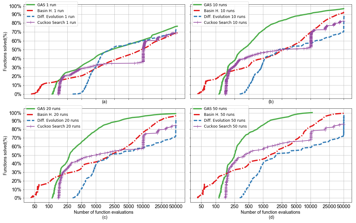
Figure 1: (Color online) To compare the performances of GAS (continuous thick line), BH (discontinuous segment-dot thick line), CS (continuous thin line with transversal segments) and DE (discontinuous segment-segment thick line) we plot the percentage of optimized test functions against the number of function reads when executing the algorithm one time (panel a). The same information is shown for concurrent optimization with 10 runs (panel b), 20 runs (panel c) and 50 runs (panel d).

As a complement to the above results, Figure 2 shows the performances of GAS, BH, CS and DE when optimizing the Lennard-Jones potentials (7) of $m=4$, $6$, $8$, and $10$ particles at randomly chosen positions (panels (a)-(d), respectively) with a single run. For the reason mentioned in Sec. 3, we expected BH to score highest in this particular benchmark but this was not the case. For $m=4$ the best performer is CS, followed by GAS and BH. For $m=6$ GAS overtakes CS while BH remains third; the performance gap between GAS and the other algorithms widens. Finally, for $m=8,10$ BH overtakes CS but it still trails GAS at a considerable distance; in both cases, the distance increases with the number of reads. DE fails badly in all cases. Let us finally remark that GAS is an unbiased algorithm, meaning that it does not exploit any specific insight into this particular optimization problem nor into any other problem, for that matter.

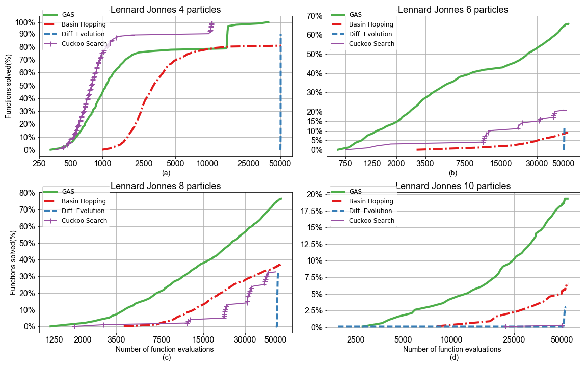
Figure 2: (Color online) Line style codification as in Fig. 1. Percentage of test functions optimized in one single run against the number of function reads for the Lennard-Jones potentials of 4 particles (panel a), 6 particles (panel b), 8 particles (panel c), and 10 particles (panel d).

5 Conclusion

In this paper we presented a general metaheuristic for the search of global extrema (GAS, Sec. 2). Among its features we highlight the use of walkers with an internal label (called flow), randomization, and cloning (i.e., the replacement of a walker or a tabu memory by a copy of another one). Numerical simulations with a representative sample of test functions (Sect. 3) shows that GAS compares favorably to Basin Hopping, Cuckoo Search, and Differential Evolution, the performance gap increasing with the number of runs in a concurrent optimization (Sec. 4). We may conclude, therefore, that GAS is a powerful tool for global optimization. The Python codes of the algorithms used in the present work as well as additional information are posted on the website [7].

ANNEX: 2D test functions

Search domains ($\mathcal{D}\subset\mathbb{R}^{2}$), global minima ($\mathbf{x}^{\ast}\in\mathcal{D}$), and minimum values of the 2D test functions (6).

1. Ackley function:

   $$\begin{array}[]{c}f_{1}(x_{1},x_{2})=-20\exp\left(-0.2\sqrt{0.5(x_{1}^{2}+x_{2}^{2})}\right)\\ -\exp\left(0.5(\cos 2\pi x_{1}+\cos 2\pi x_{2})\right)+e+20\end{array}$$

   with $\mathcal{D}=[-5,5]\times[-5,5]$, $\mathbf{x}^{\ast}=(0,0)$, and $f_{1}(\mathbf{x}^{\ast})=0$.

2. Beale function:

   $$f_{2}(x_{1},x_{2}) = (1.5-x_{1}+x_{1}x_{2})^{2}+(2.25-x_{1}+x_{1}x_{2}^{2})^{2}$$

   $$+(2.625-x_{1}+x_{1}x_{2}^{3})^{2}$$

   with $\mathcal{D}=[-4.5,4.5]\times[-4.5,4.5]$, $\mathbf{x}^{\ast}=(3,0.5)$, and $f_{2}(\mathbf{x}^{\ast})=0$.

3. Booth function:

   $$f_{3}(x_{1},x_{2})=(x_{1}+2x_{2}-7)^{2}+(2x_{1}+x_{2}-5)^{2}$$

   with $\mathcal{D}=[-10,10]\times[-10,10]$, $\mathbf{x}^{\ast}=(1,3)$, and $f_{3}(\mathbf{x}^{\ast})=0$.

4. Easom function:

   $$f_{4}(x_{1},x_{2})=-\frac{\cos x_{1}\cos x_{2}}{\exp\left((x_{1}-\pi)^{2}+(x_{2}-\pi)^{2}\right)}$$

   with $\mathcal{D}=[-100,100]\times[-100,100]$, $\mathbf{x}^{\ast}=(\pi,\pi)$, and $f_{4}(\mathbf{x}^{\ast})=-1$.

5. Eggholder function:

   $$\begin{array}[]{c}f_{5}(x_{1},x_{2})=-(x_{2}+47)\sin\sqrt{\left|\frac{x_{1}}{2}+x_{2}+47\right|}\\ -x_{1}\sin\sqrt{\left|x_{1}-(x_{2}+47)\right|}\end{array}$$

   with $\mathcal{D}=[-512,512]\times[-512,512]$, $\mathbf{x}^{\ast}=(512,404.2319)$, and $f_{5}(\mathbf{x}^{\ast})=-959.6407$.

6. Goldstein-Price function:

   $$f_{6}(x_{1},x_{2})$$

   $$= \left(1+(x_{1}+x_{2}+1)^{2}(19-14x_{1}+3x_{1}^{2}-14x_{2}+6x_{1}x_{2}+3x_{2}^{2})\right)\times$$

   $$\times\left(30+(2x_{1}-3x_{2})^{2}(18-32x_{1}+12x_{1}^{2}+48x_{2}-36x_{1}x_{2}+27x_{2}^{2})\right)$$

   with $\mathcal{D}=[-2,2]\times[-2,2]$, $\mathbf{x}^{\ast}=(0,-1)$, and $f_{6}(\mathbf{x}^{\ast})=3$.

7. Levy function N.13:

   $$\begin{array}[]{c}f_{7}(x_{1},x_{2})=\sin^{2}3\pi x_{1}+(x_{1}-1)^{2}(1+\sin^{2}3\pi x_{2})\\ +(x_{2}-1)^{2}(1+\sin^{2}2\pi x_{2})\end{array}$$

   with $\mathcal{D}=[-10,10]\times[-10,10]$, $\mathbf{x}^{\ast}=(1,1)$, and $f_{7}(\mathbf{x}^{\ast})=0$.

8. Matyas function:

   $$f_{8}(x_{1},x_{2})=0.26(x_{1}^{2}+x_{2}^{2})-0.48x_{1}x_{2}$$

   with $\mathcal{D}=[-10,10]\times[-10,10]$, $\mathbf{x}^{\ast}=(0,0)$, and $f_{8}(\mathbf{x}^{\ast})=0$.

9. McCormick function:

   $$f_{9}(x_{1},x_{2})=\sin(x_{1}+x_{2})+(x_{1}-x_{2})^{2}-1.5x_{1}+2.5x_{2}+1$$

   with $\mathcal{D}=[-1.5,4]\times[-3,4]$, $\mathbf{x}^{\ast}=(-0.54719,-1.54719)$, and $f_{9}(\mathbf{x}^{\ast})=-1.9133$.

10. Rastrigin 2D function:

    $$f_{10}(x_{1},x_{2})=20+x_{1}^{2}-10\cos 2\pi x_{1}+x_{2}^{2}-10\cos 2\pi x_{2}$$

    with $\mathcal{D}=[-5.12,5.12]\times[-5.12,5.12]$, $\mathbf{x}^{\ast}=(0,0)$, and $f_{10}(\mathbf{x}^{\ast})=0$.

11. Rosenbrock 2D function:

    $$f_{11}(x_{1},x_{2})=100(x_{2}-x_{1}^{2})^{2}+(x_{1}-1)^{2}$$

    with $\mathcal{D}=\mathbb{R}\times\mathbb{R}$, $\mathbf{x}^{\ast}=(1,1)$, and $f_{11}(\mathbf{x}^{\ast})=0$.

12. Schaffer function N. 2:

    $$f_{12}(x_{1},x_{2})=0.5+\frac{\sin^{2}(x_{1}^{2}-x_{2}^{2})-0.5}{(1+0.001(x_{1}^{2}+x_{2}^{2}))^{2}}$$

    with $\mathcal{D}=[-100,100]\times[-100,100]$, $\mathbf{x}^{\ast}=(0,0)$, and $f_{12}(\mathbf{x}^{\ast})=0$.

13. Schaffer function N. 4:

    $$f_{13}(x_{1},x_{2})=0.5+\frac{\cos^{2}\left(\sin\left|x_{1}^{2}-x_{2}^{2}\right|\right)-0.5}{(1+0.001(x_{1}^{2}+x_{2}^{2}))^{2}}$$

    with $\mathcal{D}=[-100,100]\times[-100,100]$, $\mathbf{x}^{\ast}=(0,1.25313)$, and $f_{13}(\mathbf{x}^{\ast})=0.292579$.

14. Sphere function:

    $$f_{14}(x_{1},x_{2})=x_{1}^{2}+x_{2}^{2}$$

    with $\mathcal{D}=\mathbb{R}\times\mathbb{R},$ $\mathbf{x}^{\ast}=(0,0)$, and $f_{14}(\mathbf{x}^{\ast})=0$.

15. Three-hump-camel function:

    $$f_{15}(x_{1},x_{2})=2x_{1}^{2}-1.05x_{1}^{4}+\frac{x_{1}^{6}}{6}+x_{1}x_{2}+x_{2}^{2}$$

    with $\mathcal{D}=[-5,5]\times[-5,5]$, $\mathbf{x}^{\ast}=(0,0)$, and $f_{15}(\mathbf{x}^{\ast})=0.$

References

- [1] Wales, D.J., Doye, J.P.K.: Global optimization by basin-hopping and the lowest energy structures of Lennard Jones clusters containing up to 110 atoms. Journal of Physical Chemistry A 101, 5111-5116 (1997).
- [2] Yang, X. S.: Firefly algorithms for multimodal optimization. In: Watanabe, O., Zeugmann, T. (eds.) 5th Symposium on Stochastic Algorithms, Foundation and Applications. Lectures Notes in Computer Science 5792, pp. 169–178. Springer (2009).
- [3] Storn, R., Price, K.: Differential Evolution - a simple and efficient heuristic for global optimization over continuous spaces. Journal of Global Optimization 11, 341-359 (1997).
- [4] Voss, S.: Meta-heuristics: the state of the art. In: Nareyek, A. (ed.) Local Search for Planning and Scheduling. Lecture Notes in Artifical Intelligence 2148, pp. 1-23. Springer (2001).
- [5] Kirkpatrick, S., Gelatt, C.D., Vecchi, M.P.: Optimization by simulated annealing. Science 220, issue 4598, 671-680 (1983).
- [6] Holland, J.H.: Adaptation in Natural and Artificial Systems. University of Michigan Press, Ann Arbor, 1975.
- [7] https://github.com/HCsoft-RD/Optimization.
- [8] Glover, F.: Tabu Search - Part 1. ORSA Journal on Computing 1, 190–206 (1989).
- [9] Glover, F.: Tabu Search - Part 2. ORSA Journal on Computing 2, 4–32 (1990).
- [10] Byrd, R.H., Lu, P., Nocedal, J.: A limited memory algorithm for bound constrained optimization. SIAM Journal on Scientific and Statistical Computing 16, 1190-1208 (1995).
- [11] Yang, X. S., Deb, S.: Engineering optimization by cuckoo search. Int. J. Math. Modelling Num. Optimisation, 1(4), 330–343 (2010).
- [12] Kennedy, J., Eberhart, R. C.: Particle swarm optimization. In: Proceedings of the IEEE International Conference on Neural Networks, pp. 1942–1948 (1995).