Entanglement spectrum of the degenerative ground state of Heisenberg ladders in a time-dependent magnetic field

Abstract

We investigate of the relationship between the entanglement and subsystem Hamiltonians in the perturbative regime of strong coupling between subsystems. One of the two conditions that guarantees the proportionality between these Hamiltonians obtained by using the nondegenerate perturbation theory within the first order is that the unperturbed ground state has a trivial entanglement Hamiltonian. Furthermore, we study the entanglement Hamiltonian of the Heisenberg ladders in a time-dependent magnetic field using the degenerate perturbation theory, where couplings between legs are considered as a perturbation. In this case, when the ground state is two-fold degenerate, and the entanglement Hamiltonian is proportional to the Hamiltonian of a chain within first-order perturbation theory, even then also the unperturbed ground state has a nontrivial entanglement spectrum.

I Introduction

Quantum entanglement, primarily a source of quantum information, has developed into one of the most studied subfields of many-body physics. In the last decade, quantum entanglement has mainly been used to study phase structure in condensed matter physics Amico2008 . The entanglement spectrum of a bipartite system of subsystems A and B is defined in terms of the Schmidt decomposition of its ground state $|\psi\rangle$ as

$$|\psi\rangle=\sum_{n}e^{-\frac{\xi_{n}}{2}}|\psi_{n}^{A}\rangle|\psi_{n}^{B}\rangle$$ (1)

where the states $|\psi_{n}^{A}\rangle$ ($|\psi_{n}^{B}\rangle$) are orthonormal states of the subsystem A (B), respectively, and the non-negative quantities $\xi_{n}$ represent the levels of the entanglement spectrum. Further, Haldane and Li in Ref.Li08 have reported a remarkable relationship between the excitation spectrum and the edges separating the subsystems, considering the entanglement spectrum of the fractional quantum Hall system obtained using a spatial cut. This connection between the edge spectrum and entanglement spectrum is observed in many condensed matter systems including ladders systems Qi12 ; Chen13 ; Lundgren13 In many previous studies, the proportionality between the energetic Hamiltonian of the subsystem A $\mathcal{H}_{A}$ and the entanglement Hamiltonian $\mathcal{H}_{ent}$ in the strong coupling regime POI10 ; CIR11 ; SCH11 ; PES11 ; LAE12 ; SCH12 ; SCH13 has been observed. However, this does not hold in general, even in the strong coupling limit which is illustrated by counterexamples in Ref. LUN12 where four spin terms of the Kugel-Khomskii model are considered in Ref. SCH12 , in which anisotropic spin ladders of arbitrary spin length were considered, where even the unperturbed nondegenerate ground state has a nontrivial entanglement spectrum.

Here we study the entanglement spectrum of the Heisenberg spin ladders in a time-dependent magnetic field via the degenerate perturbation theory, where couplings between legs are considered as a perturbation. The entanglement Hamiltonian is, within the first-order perturbation theory, proportional to the energy Hamiltonian of a chain in the magnetic field when the ground state is degenerate. This holds, although the entanglement spectrum of the unperturbed ground state has a nontrivial entanglement spectrum.

II Motivation

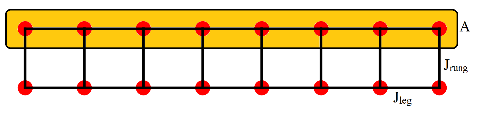
Figure 1: Illustration of the two leg spin ladder considered in this paper. The entanglement spectrum is performed by tracing out subsystem A.

We consider a bipartite system consisting of two subsystems described by Hamiltonians $\mathcal{H}_{A}$ of subsystem A and $\mathcal{H}_{B}$ of subsystem B, which are coupled by the Hamiltonian $\mathcal{H}_{0}$. We assume that the Hamiltonians $\mathcal{H}_{A}$ and $\mathcal{H}_{B}$ are small compared to $\mathcal{H}_{0}$, and it will be treated as a small perturbation. This problem can be illustrated by two leg spin ladders, where interaction between rungs is considered as a small perturbation (see Fig. 1).

The projector onto subsystem orthogonal on the nondegenerative ground state $|\psi_{0}\rangle$ is defined as

$$Q_{l}=1-|\psi_{0}\rangle\langle\psi_{0}|=\sum_{l\neq 0}|\psi_{l}\rangle\langle\psi_{l}|.$$ (2)

Then, the first correlation $|\psi_{l}^{(1)}\rangle$ of the nondegenerative ground state $|\psi_{0}\rangle$ reads

$$|\psi_{l}^{(1)}\rangle= |\psi_{0}\rangle$$

$$+ \frac{1}{E_{0}-\mathcal{H}_{0}}Q_{l}\left(\left(\mathcal{H}_{A}+\mathcal{H}_{B}\right)-\langle\psi_{0}|\left(\mathcal{H}_{A}+\mathcal{H}_{B}\right)|\psi_{0}\rangle\right)|\psi_{l}\rangle$$ (3)

where $E_{0}=\langle\psi_{0}|\mathcal{H}_{0}|\psi_{0}\rangle$. We also use that $\frac{1}{E_{0}-\mathcal{H}_{0}}Q_{l}=\sum_{l\neq 0}\frac{|\psi_{l}\rangle\langle\psi_{l}|}{E_{0}-E_{l}}$, where $E_{l}=\langle\psi_{l}|\mathcal{H}_{0}|\psi_{l}\rangle$ and the fact that $\frac{1}{E_{0}-\mathcal{H}_{0}}Q_{l}|\psi_{0}\rangle=0$ by definition. In the following, we will assume that $\frac{1}{E_{0}-E_{l}}$ is equal for every $l$. This allows us to rewrite Eq.(3) as

$$|\psi_{l}^{(1)}\rangle=|\psi_{0}\rangle+\frac{1}{E_{0}-E_{l}}(\mathcal{H}_{A}+\mathcal{H}_{B})|\psi_{0}\rangle.$$ (4)

The density matrix within the first order of the perturbation theory has the following form

$$\rho= |\psi_{l}^{(1)}\rangle\langle\psi_{l}^{(1)}|$$

$$\rho= |\psi_{0}\rangle\langle\psi_{0}|$$

$$+\frac{1}{E_{0}-E_{l}}((\mathcal{H}_{A}+\mathcal{H}_{B})|\psi_{0}\rangle\langle\psi_{0}|+|\psi_{0}\rangle\langle\psi_{0}|(\mathcal{H}_{A}+\mathcal{H}_{B})).$$ (5)

Owing to the fact that, here, the Hamiltonian $\mathcal{H}_{A}$ acts only on the subsystem A, the reduced density matrix can be calculated by tracing out the subsystem B

$$\rho_{red}=\rho_{1}+\frac{1}{E_{0}-E_{l}}\left(\mathcal{H}_{A}\rho_{1}+\rho_{1}\mathcal{H}_{A}\right)$$ (6)

where $\rho_{1}={\textrm{t}r}_{2}|\psi_{0}\rangle\langle\psi_{0}|$ is the reduced density matrix within the zeroth order of the perturbation theory. When the two subsystems are maximally entangled, $\rho_{1}$ is proportional to the unit matrix. In this case, we obtain

$$\rho_{red}=\rho_{1}\left(1-\frac{2}{E_{0}-E_{l}}\mathcal{H}_{A}\right).$$ (7)

The reduced density matrix can be reformulated as

$$\rho_{red}=\frac{1}{Z}\exp(-\mathcal{H}_{ent}^{(1)})$$ (8)

where the entanglement Hamiltonian $\mathcal{H}_{ent}$ is the entanglement Hamiltonian, and the partition function $Z$ is $Z=tr\left(exp(-\mathcal{H}_{ent}^{(1)})\right)$. The entanglement Hamiltonian

$$\mathcal{H}_{ent}=\frac{2}{E_{0}-E_{l}}\mathcal{H}_{A}$$ (9)

is proportional to the Hamiltonian of subsystem A, with the proportionality factor $\beta=\frac{2}{E_{0}-E_{l}}$ interpreted as an inverse temperature.

To conclude, we assume that

1. $\frac{1}{E_{0}-E_{l}}$ is equal for every $l$, and

2. $\rho_{1}$ is proportional to the unit matrix.

These two assumptions directly lead to the proportionality between the entanglement and subsystem Hamiltonians in the strong coupling limit within the first order of the perturbation theory, when the ground state is nondegenerate.

In Ref. POI10 , Poilblanc stressed a remarkable similarity between the chain– chain entanglement spectrum in the two-leg spin-1/2 ladders and the energy spectrum of a single spin-1/2 Heisenberg chain. Läuchli and Schliemann LAE12 analytically showed that the entanglement Hamiltonian of the two coupled anisotropic XXZ chains is proportional to the energy Hamiltonian of the single chain with renormalized anisotropy in the first order of the perturbation theory in the strong coupling limit. There, the first assumption (1) is not valid. In the case of the isotropic Heisenberg ladders, both assumptions (1) and (2) are valid, and for that reason, they found that the entanglement spectrum is directly proportional to the energy of the single chain. The authors in Ref. SCH12 generalized this observation for the isotropic Heisenberg ladders to the case of the arbitrary spin length S. They found that for arbitrary spin, the entanglement spectrum of the isotropic Heisenberg ladders is proportional to the energy of the single chain within the first-order perturbation theory. This is also a consequence of the fact that both assumptions (1) and (2) hold. However, they found that there is no proportionality between the entanglement Hamiltonian of anisotropic spin ladders of arbitrary spin length. Since here, the reduced density matrix in zeroth order of the perturbation theory is not proportional to the unit matrix, there is no mention of proportionality.

III Model

We investigate the Hamiltonian of the Heisenberg spin-1/2 ladder in a time-dependent circularly polarized magnetic field $B$ described by the Hamiltonian

$$\tilde{H} =J_{rung}\sum_{i}\vec{S}_{2i}\vec{S}_{2i+1}+B\sum_{i}\left(S_{i}^{x}\cos\omega t-S_{i}^{y}\sin\omega t\right)$$

$$+J_{leg}\sum_{i}\vec{S}_{2i}\vec{S}_{2i+2}+J_{leg}\sum_{i}\vec{S}_{2i+1}\vec{S}_{2i+3}.$$ (10)

where $\omega$ is the angular velocity of the rotation of the magnetic field. The sites on the first (second) leg are denoted by even (odd) labels, such that the $i$th rung consists of sites $2i$ and $2i+1$. All spin-1/2 operators are taken to be dimensionless, such that the couplings along the rungs $J_{rung}$ and the legs $J_{leg}$ have the dimensions of energy. We will consider antiferromagnetic coupling when $J_{rung}>0$.

This time-dependent Hamiltonian can be factorized to a time-independent Hamiltonian by unitary transformations that represent a rotation around the z-axis $R(t)=\exp(-iS_{z}\omega t/\hbar)$ QT . Since

$$R(t)S_{x}R^{-1}(t)=S_{x}\cos\omega t+S_{y}\sin\omega t$$

$$R(t)S_{y}R^{-1}(t)=-S_{x}\sin\omega t+S_{y}\cos\omega t$$

$$R(t)S_{z}R^{-1}(t)=S_{z}$$ (11)

Hamiltonian Eq. (10) can be transformed into a time-independent Hamiltonian

$$\widehat{H} =R(t)\tilde{H}(t)R(t)^{-1}$$ (12)

$$\widehat{H} =J_{rung}\sum_{i}\vec{S}_{2i}\vec{S}_{2i+1}+B\sum_{i}S_{i}^{x}+J_{leg}\sum_{i}\vec{S}_{2i}\vec{S}_{2i+2}$$

$$+J_{leg}\sum_{i}\vec{S}_{2i+1}\vec{S}_{2i+3}.$$ (13)

Defining the propagator that confirms

$$\frac{\partial}{\partial t}K(t,t_{0})=-\frac{i}{\hbar}\tilde{H}(t)K(t,t_{0})$$ (14)

$$\frac{\partial}{\partial t}K(t,t_{0})=-\frac{i}{\hbar}R_{-1}(t)\widehat{H}(t)R(t)K(t,t_{0})$$ (15)

we find

$$\frac{\partial}{\partial t}\left(R(t)K(t,t_{0})R^{-1}(t_{0})\right)=-\frac{i}{\hbar}H\left(R(t)K(t,t_{0})R^{-1}(t_{0})\right).$$

Then, the Hamiltonian becomes

$$H= J_{rung}\sum_{i}\vec{S}_{2i}\vec{S}_{2i+1}+B\sum_{i}S_{i}^{x}+\omega\sum_{i}S_{i}^{z}$$

$$+ J_{leg}\sum_{i}\vec{S}_{2i}\vec{S}_{2i+2}+J_{leg}\sum_{i}\vec{S}_{2i+1}\vec{S}_{2i+3}$$ (16)

where the propagator is

$$K(t,t_{0})=\exp\left(\frac{i}{\hbar}S_{z}\omega t\right)\exp\left(-\frac{i}{\hbar}H(t-t_{0})\right)\exp\left(-\frac{i}{\hbar}S_{z}\omega t_{0}\right).$$ (17)

In order to use the perturbation theory, we will rewrite the Hamiltonian Eq.(16) as $H=H_{0}+H_{1}$ where

$$H_{0}=J_{rung}\sum_{i}\vec{S}_{2i}\vec{S}_{2i+1}+B\sum_{i}S_{i}^{x}+\omega\sum_{i}S_{i}^{z}$$ (18)

and

$$H_{1}=J_{leg}\sum_{i}\vec{S}_{2i}\vec{S}_{2i+2}+J_{leg}\sum_{i}\vec{S}_{2i+1}\vec{S}_{2i+3}$$ (19)

and consider $H_{1}$ as a small perturbation. The Hamiltonian Eq.(18) is independent of the direction of the magnetic field and it can be considered as the isotropic Heisenberg chain in the magnetic field $\sqrt{B^{2}+\omega^{2}}$

$$H_{0} =J_{rung}\sum_{i}\vec{S}_{2i}\vec{S}_{2i+1}+\sqrt{B^{2}+\omega^{2}}\sum_{i}S_{i}^{z}$$ (20)

and

$$H_{1} =J_{leg}\sum_{i}\vec{S}_{2i}\vec{S}_{2i+2}+J_{leg}\sum_{i}\vec{S}_{2i+1}\vec{S}_{2i+3}.$$ (21)

The energies of a rung of the singlet and triplet states are

$$E_{s_{i}}=-\frac{3}{4}J_{rung}$$ (22)

$$E_{t_{i}^{+}}=\frac{1}{4}J_{rung}+\sqrt{B^{2}+\omega^{2}}$$ (23)

$$E_{t_{i}^{0}}=\frac{1}{4}J_{rung}$$ (24)

$$E_{t_{i}^{-}}=\frac{1}{4}J_{rung}-\sqrt{B^{2}+\omega^{2}},$$ (25)

The ground state changes from the spin singlet $|s_{i}\rangle$, to the triplet state $|t^{-}_{i}\rangle$ by increasing the value of $\sqrt{B^{2}+\omega^{2}}$ . When $J_{rung}=\sqrt{\omega^{2}+B^{2}}$, the ground state is two-fold degenerate, since the singlet states $|s_{i}\rangle$ and triplet states $|t_{i}^{-}\rangle$ have the same eigenenergy. The situation when ground state is two-fold degenerate is quite interesting and it will be considered in the following section.

IV Entanglement spectrum

When $J_{rung}=\sqrt{\omega^{2}+B^{2}}$, it is necessary to use degenerate perturbation theory, while any combination of eigenstates $|s_{i}\rangle$ and $|t_{i}^{-}\rangle$ can be taken as the ground state $|\psi_{0}\rangle$. In order to achieve an analytically manageable situation, we will assume a finite number of rungs $i=4$. Let us suppose that the unperturbed ground state $|psi_{0}\rangle$ of the Hamiltonian $\mathcal{H}_{0}$ is an unknown combination of eigenvectors $|s_{i}\rangle$ and $|t_{i}^{-}\rangle$. In the following, we will note eigenvectors of the ground state $|\psi_{0}\rangle$ as $\{|\overline{n}\lambda\rangle|,\lambda=1,...,4\}$, where

$$|\overline{n}1\rangle=|s_{1}\rangle|s_{2}\rangle|s_{3}\rangle|s_{4}\rangle,|\overline{n}2\rangle=|s_{1}\rangle|s_{2}\rangle|s_{3}\rangle|t_{4}^{-}\rangle,$$

$$|\overline{n}3\rangle=|s_{1}\rangle|s_{2}\rangle|t_{3}^{-}\rangle|s_{4}\rangle,|\overline{n}4\rangle=|s_{1}\rangle|t_{2}^{-}\rangle|s_{3}\rangle|s_{4}\rangle,$$

$$|\overline{n}5\rangle=|t_{1}^{-}\rangle|s_{2}\rangle|s_{3}\rangle|s_{4}\rangle,|\overline{n}6\rangle=|t_{1}^{-}\rangle|t_{2}^{-1}\rangle|s_{3}\rangle|s_{4}\rangle,$$

$$|\overline{n}7\rangle=|t_{1}^{-1}\rangle|s_{2}\rangle|t_{3}^{-1}\rangle|s_{4}\rangle,|\overline{n}8\rangle=|t_{1}^{-1}\rangle|s_{2}\rangle|s_{3}\rangle|t_{4}^{-1}\rangle,$$

$$|\overline{n}9\rangle=|s_{1}\rangle|t_{2}^{-1}\rangle|t_{3}^{-1}\rangle|s_{4}\rangle,|\overline{n}10\rangle=|s_{1}\rangle|t_{2}^{-1}\rangle|s_{3}\rangle|t_{4}^{-1}\rangle,$$

$$|\overline{n}11\rangle=|s_{1}\rangle|s_{2}\rangle|t_{3}^{-1}\rangle|t_{4}^{-1}\rangle,|\overline{n}12\rangle=|t_{1}^{-1}\rangle|t_{2}^{-1}\rangle|t_{3}^{-1}\rangle|s_{4}\rangle,$$

$$|\overline{n}13\rangle=|t_{1}^{-1}\rangle|t_{2}^{-1}\rangle|s_{3}\rangle|t_{4}^{-1}\rangle,|\overline{n}14\rangle=|t_{1}^{-1}\rangle|s_{2}\rangle|t_{3}^{-1}\rangle|t_{4}^{-1}\rangle,$$

$$|\overline{n}15\rangle=|s_{1}\rangle|t_{2}^{-1}\rangle|t_{3}^{-1}\rangle|t_{4}^{-1}\rangle,|\overline{n}16\rangle=|t_{1}^{-1}\rangle|t_{2}^{-1}\rangle|t_{3}^{-1}\rangle|t_{4}^{-1}\rangle$$ (26)

The projector $P_{n}^{(0)}$ of $\mathcal{H}_{0}$ projects on the subspace, and is defined by the eigenvalue $E_{\overline{n}}^{(0)}=-\frac{3}{4}J_{rung}$ of the Hamiltonian $\mathcal{H}_{0}$. Furthermore, the projector $P_{n}^{(0)}$ satisfies

$$P_{n}^{(0)}\mathcal{H}^{{}^{\prime}}P_{n}^{(0)}|\psi_{0}\rangle=E^{(1)}|\psi_{0}\rangle$$ (27)

where $E^{(1)}$ is the eigenvalue of $P_{n}^{(0)}\mathcal{H}^{{}^{\prime}}P_{n}^{(0)}$ for eigenvector $|\psi_{0}\rangle$. In order to find the eigenvalue $E^{(1)}$ of the perturbation $\mathcal{H^{{}^{\prime}}}$ and the ground state $|\psi_{0}\rangle$, it is sufficient to diagonalize a $16\times 16$ matrix

$$\left[\begin{array}[]{ccc}\langle\overline{n}1|\mathcal{H}^{{}^{\prime}}|\overline{n}1\rangle&\cdot\cdot\cdot&\langle\overline{n}1|\mathcal{H}^{{}^{\prime}}|\overline{n}16\rangle\\ \cdot\cdot\cdot&\cdot\cdot\cdot&\cdot\cdot\cdot\\ \langle\overline{n}16|\mathcal{H}^{{}^{\prime}}|\overline{n}1\rangle&\cdot\cdot\cdot&\langle\overline{n}16|\mathcal{H}^{{}^{\prime}}|\overline{n}16\rangle\end{array}\right].$$ (28)

By elementary calculations, one finds the uniquely determined ground state $|\psi_{0}\rangle$ and the first correction of the energy $E^{(1)}$.

The unperturbed density matrix is constructed from this ground state and is given, after simplification, by

$$\rho^{(0)}= \sum_{\lambda}^{16}|\overline{n}\lambda\rangle\langle\overline{n}\lambda|.$$ (29)

By again tracing out one leg, we obtain the reduced unperturbed density matrix

$$\rho_{red}^{(0)}=\frac{1}{2^{4}}\bigotimes_{i=1}^{4}\left(1-S_{2i+1}^{z}\right)$$ (30)

It is obvious that this reduced density matrix is not proportional to the unitary matrix and possesses a nontrivial entanglement spectrum. The first corrections to the ground state in the degenerate perturbation theory are defined by

$$|1\rangle= \sum_{n\neq\overline{n}}|n\lambda\rangle\frac{\langle n\lambda|H_{1}|\psi_{0}\rangle}{E_{\overline{n}}^{(0)}-E_{n}^{(0)}},$$ (31)

$$|1^{{}^{\prime}}\rangle= \sum_{n\neq\overline{n},n^{\prime}}\sum_{\lambda^{\prime}}|\overline{n}\lambda\rangle\frac{\langle\overline{n}\lambda|H_{1}|n^{\prime}\lambda\rangle}{E^{(1)}-E_{\lambda}^{(1)}}\frac{\langle n^{\prime}\lambda|H_{1}|\psi_{0}\rangle}{E_{\overline{n}}^{(0)}-E_{n^{\prime}}^{(0)}}.$$ (32)

One finds the reduced density matrix to the first order

$$\rho_{red}^{(1)}= \frac{1}{2^{4}}\bigotimes_{i=1}^{4}\left(1-S_{2i+1}^{z}\right)-\frac{J_{leg}}{8J_{rung}}\left((1-S_{1}^{z})(1-S_{3}^{z})\vec{S}_{5}\vec{S}_{7}\right.$$

$$+ \left.(1-S_{1}^{z})\vec{S}_{3}\vec{S}_{5}(1-S_{7}^{z})+\vec{S}_{1}\vec{S}_{3}(1-S_{5}^{z})(1-S_{7}^{z})\right)$$ (33)

The reduced density matrix can be rewritten as

$$\rho_{red}=\frac{1}{Z}\exp(-\mathcal{H}_{ent}^{(1)})$$ (34)

where the partition function $Z$ is $Z=\textrm{tr}\exp(-\mathcal{H}_{ent}^{(1)})$ and the entanglement Hamiltonian within the first order of the perturbation theory has the following form

$$\mathcal{H}_{ent}^{(1)}=\frac{1}{J_{rung}}\sum_{i=0}^{3}\left(2J_{leg}\vec{S}_{2i+1}\vec{S}_{2i+3}+J_{rung}S_{2i+1}\right).$$ (35)

The entanglement Hamiltonian is simply proportional to the Hamiltonian of a chain in the magnetic field with the proportional factor $\beta=\frac{1}{J_{rung}}$ defined as an inverse temperature.

The system of the Heisenberg chain in the longitudinal magnetic field is exactly solvable by the Bethe ansatz. The ground state becomes the spin–liquid one and gapless up to when $\frac{\sqrt{B^{2}+\omega^{2}}}{J_{leg}}=2$, where the phase transition of the Pokrovsky–Talapov type takes place and the ground state becomes a completely ordered gapped ferromagnetic state. One of the most important features of the energy spectra of spin chains is the absence of an excitation gap over the ground state for the integer spin length. We restrict ourselves to the case when the two chains are strongly coupled; therefore, $\frac{\sqrt{B^{2}+\omega^{2}}}{J_{leg}}>>1$ and the Hamiltonian of a subsystem stays gapless in this region. The entanglement spectrum Eq.(35) remains gapless owing to the proportionality to the energy spectrum.

V Summary

Here we investigated the entanglement spectrum of Heisenberg ladders in a time-dependent magnetic field using the degenerate perturbation theory, where couplings between legs are taken as a small perturbation. When the ground state is not degenerate, the existence of the trivial entanglement Hamiltonian in the zeroth order of the perturbation theory is identified as an important condition that guarantees the proportionality between the entanglement and subsystem Hamiltonians. We find that although the entanglement spectrum of the unperturbed ground state has a nontrivial entanglement spectrum, the entanglement Hamiltonian of Heisenberg ladders in a time-dependent magnetic field, within the first-order perturbation theory, is proportional to the energy Hamiltonian of a chain in the magnetic field when the ground state is degenerate.

VI ACKNOWLEDGMENTS

The author kindly acknowledges John Schliemann.

References

• (1) Luigi Amico, Rosario Fazio, Andreas Osterloh, and Vlatko Vedral, Rev. Mod. Phys. 80, 517 (2008).
• (2) H. Li and F.Β D.Β M. Haldane, Phys. Rev. Lett. 101, 010504 (2008).
• (3) Xiao-Liang Qi, Hosho Katsura, and Andreas W. W. Ludwig, Phys. Rev. Lett. 108, 196402 (2012).
• (4) Xiao Chen, and Eduardo Fradkin J. Stat. Mech. (2013) P08013.
• (5) Rex Lundgren, Yohei Fuji, Shunsuke Furukawa, and Masaki Oshikawa, Phys. Rev. B 88, 245137 (2013).
• (6) D. Poilblanc, Phys. Rev. Lett. 105, 077202 (2010).
• (7) J. I. Cirac, D. Poilblanc, N. Schuch and F. Verstraete, Phys. Rev. B 83, 245134 (2011).
• (8) J. Schliemann, Phys. Rev. B 83, 115322 (2011).
• (9) Ingo Peschel and Ming-Chiang Chung, Europhys. Lett. 96, 50006 (2011).
• (10) A. M. LΓ€uchli and J. Schliemann, Phys. Rev. B 85, 054403 (2012).
• (11) J. Schliemann and A. M . LΓ€uchli, J. Stat. Mech. P11021 (2012).
• (12) J. Schliemann, New J. Phys 15, 053017 (2013).
• (13) R. Lundgren, V. Chua, and G. A. Fiete, Phys. Rev. B 86, 224422 (2012).
• (14) Thomas Dittrich, Peter HΓ€nggi, Gert-Ludwig Ingold, Bernhard Kramer, Gerd SchΓΆn, and Wilhelm Zwerger, Wiley-VCH, Weinheim (1998).