Stochastic decomposition applied to
large-scale hydro valleys management

Abstract

We are interested in optimally controlling a discrete time dynamical system that can be influenced by exogenous uncertainties. This is generally called a Stochastic Optimal Control (SOC) problem and the Dynamic Programming (DP) principle is one of the standard way of solving it. Unfortunately, DP faces the so-called curse of dimensionality: the complexity of solving DP equations grows exponentially with the dimension of the variable that is sufficient to take optimal decisions (the so-called state variable). For a large class of SOC problems, which includes important practical applications in energy management, we propose an original way of obtaining near optimal controls. The algorithm we introduce is based on Lagrangian relaxation, of which the application to decomposition is well-known in the deterministic framework. However, its application to such closed-loop problems is not straightforward and an additional statistical approximation concerning the dual process is needed. The resulting methodology is called Dual Approximate Dynamic Programming (DADP). We briefly present DADP, give interpretations and enlighten the error induced by the approximation. The paper is mainly devoted to applying DADP to the management of large hydro valleys. The modeling of such systems is presented, as well as the practical implementation of the methodology. Numerical results are provided on several valleys, and we compare our approach with the state of the art SDDP method.

1 Introduction

1.1 Large-scale systems and energy applications

Consider a controlled dynamical system over a discrete and finite time horizon. This system may be influenced by exogenous noises that affect its behavior. We suppose that, at every instant, the decision maker is able to observe the noises and to keep these observations in memory. Since it is generally profitable to take available observations into account when designing future decisions, we are looking for strategies rather than simple decisions. Such strategies (or policies) are feedback functions that map every instant and every possible history of the system to a decision to be made.

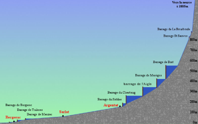
Figure 1: The Dordogne river.

The typical applications we have in mind are in the field of energy management. Consider a power producer that owns a certain number of power units. Each unit has its own local characteristics such as physical constraints that restrain the set of feasible decisions, and induces a production cost or a revenue. The power producer has to control the power units so that an overall goal is met. A classical example is the so-called unit commitment problem Takriti et al. [1996] where the producer has to satisfy a global power demand at every instant. The power demand, as well as other parameters such as unit breakdowns, are random. The producer is looking for strategies that make the overall production cost minimal, over a given time horizon. Another application, which is considered in this paper, is the management of a large-scale hydro valley: here the power producer manages a cascade of dams, and maximizes the revenue obtained by selling the energy produced by turbinating the water inside the dams. Both natural inflows in water reservoirs and prices are random. In all these problems, both the number of power units and the number of time steps are usually large de Matos et al. [2015].

1.2 Standard resolution methods

One classical approach when dealing with stochastic dynamic optimization problems is to discretize the random inputs of the problem using a scenario tree. Such an approach has been widely studied within the stochastic programming community (Heitsch & Römisch [2009], Shapiro et al. [2009]), and also used to model and solve energy problems Pflug & Pichler [2014]. One of the advantages of such a technique is that, as soon as the scenario tree is drawn, the derived problem can be treated by classical mathematical programming techniques. Thus, a number of decomposition methodologies have been proposed (see for instance Rockafellar & Wets [1991], Carpentier et al. [1996], Ruszczyński [1997], [Ruszczyński & Shapiro, 2003, Chap. 3]) and applied to energy planning problems Bacaud et al. [2001]. The way to combine the discretization of expectation together with the discretization of information in a general setting has been presented in Heitsch et al. [2006], Carpentier et al. [2015] and Pflug & Pichler [2014]). However, in a multi-stage setting, this methodology suffers from the drawback that arises with scenario trees: as it was pointed out by Shapiro [2006], the number of scenarios needed to achieve a given accuracy grows exponentially with the number of time steps of the problem.

The other natural approach to solve SOC problems is to rely on the dynamic programming (DP) principle (see Bellman [1957], Puterman [1994], Bertsekas [2000]). The core of the DP approach is the definition of a state variable that is, roughly speaking, the variable that, in conjunction with the time variable, is sufficient to take an optimal decision at every instant. It does not have the drawback of the scenario trees concerning the number of time steps since strategies are, in this context, depending on a state variable whose space dimension does not grow with time. However, DP suffers from another drawback which is the so-called curse of dimensionality: the complexity of solving the DP equation grows exponentially with the state space dimension. Hence, solving the DP equation by brute force is generally intractable when the state space dimension goes beyond several units. In Vezolle et al. [2009], the authors were able to solve DP on a $10$ state variables energy management problem, using parallel computation coupled with adequate data distribution, but the DP limits are around $5$ state variables in a straightforward use of the method.

Another popular idea is to represent the value functions (solutions of the DP equation) as a linear combination of a priori chosen basis functions (see Bellman & Dreyfus [1959] Bertsekas & Tsitsiklis [1996]). This approach, called Approximate Dynamic Programming (ADP) has become very popular and the reader is referred to Powell [2011] and Bertsekas [2012] for a precise description of ADP. This approximation drastically reduces the complexity of solving the DP equation. However, in order to be practically efficient, such an approach requires some a priori information about the problem, in order to define a well suited functional subspace. Indeed, there is no systematic means to choose the basis functions and several choices have been proposed in the literature Tsitsiklis & Van Roy [1996].

Last but not least is the popular DP-based method called Stochastic Dual Dynamic Programming (SDDP). Starting with the seminal work Van Slyke & Wets [1969], the SDDP method has been designed in Pereira & Pinto [1991]. It has been widely used in the energy management context and lately regained interest in the Stochastic Programming community Philpott & Guan [2008], Shapiro [2011]. The idea is somehow to extend Kelley’s cutting plane method to the case of multi-stage problems. Alternatively it can be seen as a multistage Benders (or L-shaped) decomposition method with sampling. It consists in a succession of forward (simulation) and backward (Bellman function refining) passes that ultimately aim at approaching the Bellman function by the supremum of affine hyperplanes (cuts) generated during the backward passes. It provides an efficient alternative to simply discretizing the state space to solve the DP equation. In the convex case with finite support random variables, it has been proven by Girardeau et al. [2015] that the method converges to optimality.

1.3 Decomposition approach

When dealing with large-scale optimization problems, the decomposition-coordination approach aims at finding a solution to the original problem by iteratively solving subproblems of smaller dimension. In the deterministic case, several types of decomposition have been proposed (e.g. by prices, by quantities or by interaction prediction) and unified in Cohen [1980] using a general framework called Auxiliary Problem Principle. In the open-loop stochastic case, i.e. when controls do not rely on any observation, it is proposed in Cohen & Culioli [1990] to take advantage of both decomposition techniques and stochastic gradient algorithms.

The natural extension of these techniques in the closed-loop stochastic case (see Barty et al. [2009]) fails to provide decomposed state dependent strategies. Indeed, the optimal strategy of a subproblem depends on the state of the whole system, and not only on the local state. In other words, decomposition approaches are meant to decompose the control space, namely the range of the strategy, but the numerical complexity of the problems also arises because of the dimensionality of the state space, that is to say the domain of the strategy.

We recently proposed a way to use price decomposition within the closed-loop stochastic case. The coupling constraints, namely the constraints preventing the problem from being naturally decomposed, are dualized using a Lagrange multiplier (price). At each iteration, the price decomposition algorithm solves each subproblem using the current price, and then uses the solutions to update it. In the stochastic context, the price is a random process whose dynamics is not available, so the subproblems do not in general fall into the Markovian setting. However, in a specific instance of this problem Strugarek [2006], the author exhibited a dynamics for the optimal multiplier and showed that these dynamics were independent with respect to the decision variables. Hence it was possible to come down to the Markovian framework and to use DP to solve the subproblems in this case. Following this idea, it is proposed in Barty et al. [2010b] to choose a parameterized dynamics for these multipliers in such a way that solving subproblems using DP becomes possible. While the approach, called Dual Approximate Dynamic Programming (DADP), showed promising results on numerical examples, it suffers from the fact that the induced restrained dual space is non-convex, leading to some numerical instabilities. Moreover, it was not possible to give convergence results for the algorithm.

The method has then been improved through a series of PhD theses (Girardeau [2010], Alais [2013] and Leclère [2014]) both from the theoretical and from the practical point of view. The methodology still relies on Lagrangian decomposition. In order to make the resolution of subproblems tractable, the core idea is to replace the current Lagrange multiplier by its conditional expectation with respect to some information process, at every iteration. This information process has to be a priori chosen and adapted to the natural filtration. Assume that the information process is driven by a dynamics: the state in each subproblem then consists of the original state augmented by the new state induced by the information process, making the resolution of the subproblem tractable by DP. The quality of the results produced by the algorithm highly depends on the choice of this information variable. An interesting point is that approximating the multipliers by their conditional expectations has an interpretation in terms of a relaxed optimization problem: this revisited DADP algorithm in fact aims at solving an approximate primal problem where the almost-sure coupling constraint has been replaced by its conditional expectation with respect to the information variable. In other words, this methodology consists in solving a relaxed primal problem, hence giving a lower bound of the true optimal cost. Another consequence of this approximation is that the solutions obtained by the DADP algorithm do not satisfy the initial almost-sure coupling constraint, so we must rely on a heuristic procedure to produce a feasible solution to the original problem.

1.4 Contents of the paper

The main contribution of the paper is to give a practical algorithm aiming at solving large scale stochastic optimal control problems and providing closed-loop strategies. The numerous approximations used in the algorithm, and especially the one allowing for feasible strategies, make difficult to theoretically assess the quality of the solution finally adopted. Nevertheless, numerical implementation shows that the method is promising to solve large scale optimization problems such as those encountered in the field of energy management.

The paper is organized as follows. In §2, we present the hydro valley management problem, the corresponding general SOC formulation and the DP principle. We then concentrate on the spatial decomposition of such a problem and the difficulties of using DP at the subproblem level. In §3, we present the DADP method and give different interpretations. We then propose a way to recover an admissible solution from the DADP results and we briefly discuss the theoretical and practical questions associated to the convergence and implementation of the method. Finally, in §4, we apply the DADP method to the management of hydro valleys. Different examples, corresponding to either academic or realistic valleys, are described. A comparison of the method with SDDP is outlined.

1.5 Notations

We will use the following notations, considering a probability space $(\Omega,\mathscr{A},\mathbb{P})$:

• bold letters for random variables, normal font for their realizations;

• ${\boldsymbol{X}}\preceq\mathcal{F}_{t}$ (resp. ${\boldsymbol{X}}\preceq{\boldsymbol{Y}}$) means that the random variable ${\boldsymbol{X}}$ is measurable with respect to the $\sigma$-algebra $\mathcal{F}_{t}$ (resp. with respect to the $\sigma$-algebra generated by ${\boldsymbol{Y}}$, denoted by $\sigma({\boldsymbol{Y}})$);

• $x$ generally stands for the state, $u$ for the control, $w$ for an exogeneous noise;

• $L_{t}$ for a cost function at time $t$, $K$ for a final cost function;

• $V_{t}$ represent a Bellman’s value function at time $t$;

• $\llbracket i,j\rrbracket$ is the set of integer between $i$ and $j$;

• the notation ${\boldsymbol{X}}^{i}$ (resp. ${\boldsymbol{U}}^{i}$ and ${\boldsymbol{Z}}^{i}$) stands for the discrete time state process $({\boldsymbol{X}}_{0}^{i},\ldots,{\boldsymbol{X}}_{T}^{i})$ (resp. control processes $({\boldsymbol{U}}_{0}^{i},\ldots,{\boldsymbol{U}}_{T-1}^{i})$, $({\boldsymbol{Z}}_{0}^{i},\ldots,{\boldsymbol{Z}}_{T-1}^{i})$).

2 Mathematical formulation

In this section, we present the modeling of a hydro valley and the associated optimization framework.

2.1 Dams management problem

We consider a hydro valley constituted of $N$ cascaded dams as represented in Figure 2. The water turbinated at a dam produces energy which is sold on electricity markets, and then enters the nearest downstream dam.

Figure 2: Operating scheme of a hydro valley with $3$ dams.

We formulate the problem of maximizing the cascade revenue over a discrete time horizon $\{0,1,\ldots,T\}$. The representative variables of dam $i$ at time $t$ are: $u_{t}^{i}$ for the water turbinated, $x_{t}^{i}$ for the current water volume, $a_{t}^{i}$ for the natural water inflow entering dam $i$, $p_{t}^{i}$ for the market value of the water of dam $i$. The randomness is given by $w_{t}^{i}=(a_{t}^{i},p_{t}^{i})$.

The modeling of a dam takes into account a possible overflow: the spilled water does not produce electricity, but enters the next dam (see Figure 3).

Figure 3: Dam behavior.

• The dam dynamics reads

  $$x_{t+1}^{i} =x_{t}^{i}-u_{t}^{i}+a_{t}^{i}+z_{t}^{i}-s_{t}^{i}=f_{t}^{i}(x_{t}^{i},u_{t}^{i},w_{t}^{i},z_{t}^{i})\;,$$

  where $s_{t}^{i}$ is the volume of water spilled by overflow of the dam:

  $$s_{t}^{i}=\max\big{\{}0,x_{t}^{i}-u_{t}^{i}+a_{t}^{i}+z_{t}^{i}-\overline{x}^{i}\big{\}}\;.$$

  The constant value $\overline{x}^{i}$ stands for the maximal capacity of dam $i$. The outflow of dam $i$, that is, the sum of the turbinated water and of the spilled water, is denoted by $z_{t}^{i+1}$:

  $$z_{t}^{i+1} =u_{t}^{i}+s_{t}^{i}=g_{t}^{i}(x_{t}^{i},u_{t}^{i},w_{t}^{i},z_{t}^{i})\;.$$

  Note that these dynamic equations are nonlinear because of the $\max$ operator in the definition of the spilled water volume. We assume the Hazard-Decision information structure: the control $u_{t}^{i}$ applied at time $t$ is chosen once the noise $w_{t}^{i}$ at time $t$ has been observed. It is thus possible to ensure that the dam always remains above its minimal admissible volume $\underline{x}^{i}$ by limiting the control range:

  $$\underline{u}^{i}\leq u_{t}^{i}\leq\min\big{\{}\overline{u}^{i},x_{t}^{i}+a_{t}^{i}+z_{t}^{i}-\underline{x}^{i}\big{\}}\;.$$

  Remark 1.

  As will be seen in §4, the typical time step length we use is the month (with a time horizon of one year). It is thus reasonable to assume the hazard-decision framework, the control applied for a given month being in fact implemented each day taking into account the observed information on a daily basis.

• The gain of the dam is the sum of different terms.

  • Gain at each time $t<T$:

    $$p_{t}^{i}u_{t}^{i}-\epsilon(u_{t}^{i})^{2}\;;$$

    we denote by $L_{t}^{i}(x_{t}^{i},u_{t}^{i},w_{t}^{i},z_{t}^{i})$ the opposite of this gain (cost). The quadratic terms $\epsilon(u_{t}^{i})^{2}$ ensure the strong convexity of the cost function. These terms model the operating cost of the turbine and are usually small.

  • Final gain at time $T$:

    $$-a^{i}\min\{0,x_{T}^{i}-\widehat{x}^{i}\}^{2}\;;$$

    we again denote by $K^{i}\big{(}x_{T}^{i}\big{)}$ the opposite of this gain. It corresponds to a quadratic penalization around a target value $\widehat{x}^{i}$ representing the desired water volume in the dam at the end of the time horizon.

  Taking into account the opposite of the gains, we thus have to deal with a minimization problem.

Thus the global optimization problem reads

$$\min_{({\boldsymbol{X}},{\boldsymbol{U}},{\boldsymbol{Z}})}\quad \mathbb{E}\bigg{(}\sum_{i=1}^{N}\Big{(}\sum_{t=0}^{T-1}L_{t}^{i}\big{(}{\boldsymbol{X}}_{t}^{i},{\boldsymbol{U}}_{t}^{i},{\boldsymbol{W}}_{t}^{i},{\boldsymbol{Z}}_{t}^{i}\big{)}+K^{i}\big{(}{\boldsymbol{X}}_{T}^{i}\big{)}\Big{)}\bigg{)}\;,$$ (1a)

$$s.t.\qquad {\boldsymbol{X}}^{i}_{0}\quad\text{given}\;,$$

$${\boldsymbol{X}}_{t+1}^{i}=f_{t}^{i}({\boldsymbol{X}}_{t}^{i},{\boldsymbol{U}}_{t}^{i},{\boldsymbol{W}}_{t}^{i},{\boldsymbol{Z}}_{t}^{i})\;,\enspace i\in\llbracket 1,N\rrbracket\;,\enspace t\in\llbracket 0,T-1\rrbracket\;,$$ (1b)

$${\boldsymbol{U}}_{t}^{i}\preceq\sigma({\boldsymbol{W}}_{0},\ldots,{\boldsymbol{W}}_{t})\;,\enspace\qquad\>\>i\in\llbracket 1,N\rrbracket\;,\enspace t\in\llbracket 0,T-1\rrbracket\;,$$ (1c)

$${\boldsymbol{Z}}^{1}_{t}=0\;,$$

$${\boldsymbol{Z}}_{t}^{i+1}=g_{t}^{i}({\boldsymbol{X}}_{t}^{i},{\boldsymbol{U}}_{t}^{i},{\boldsymbol{W}}_{t}^{i},{\boldsymbol{Z}}_{t}^{i})\;,\enspace i\in\llbracket 1,N\rrbracket\;,\enspace t\in\llbracket 0,T-1\rrbracket\;.$$ (1d)

Equations (1c) represent the so-called non-anticipativity constraints, that is, the fact that each control ${\boldsymbol{U}}_{t}^{i}$, considered as a random variable, has to be measurable with respect to the sigma-field $\sigma({\boldsymbol{W}}_{0},\ldots,{\boldsymbol{W}}_{t})$ generated by the noise sequence $({\boldsymbol{W}}_{0},\ldots,{\boldsymbol{W}}_{t})$ up to time $t$.

2.2 A more generic formulation

With a slight abuse of notation, the stochastic optimization problem formulated at §2.1 reads

$$\min_{({\boldsymbol{X}}^{i},{\boldsymbol{U}}^{i})_{i\in\llbracket 1,N\rrbracket}}\; \mathbb{E}\bigg{(}\sum_{i=1}^{N}\Big{(}\sum_{t=0}^{T-1}L^{i}_{t}({\boldsymbol{X}}^{i}_{t},{\boldsymbol{U}}^{i}_{t},{\boldsymbol{W}}_{t})+K^{i}({\boldsymbol{X}}^{i}_{T})\Big{)}\bigg{)}\;,$$ (2a)

s.t. $${\boldsymbol{X}}^{i}_{t+1}=f^{i}_{t}({\boldsymbol{X}}^{i}_{t},{\boldsymbol{U}}^{i}_{t},{\boldsymbol{W}}_{t})\;,\quad{\boldsymbol{X}}^{i}_{0}\quad\text{given}\;,$$ (2b)

$${\boldsymbol{U}}^{i}_{t}\preceq\sigma({\boldsymbol{W}}_{0},\ldots,{\boldsymbol{W}}_{t})\;,$$ (2c)

$$\sum_{i=1}^{N}\Theta^{i}_{t}({\boldsymbol{X}}^{i}_{t},{\boldsymbol{U}}^{i}_{t},{\boldsymbol{W}}_{t})=0\;.$$ (2d)

Constraints (2b) represent the dynamics and constraints (2c) are the non-anticipativity constraints. The last constraints (2d) express the interactions between the dams in a more general way than Equations (1d). They represent an additive coupling with respect to the different production units, which is termed the “spatial coupling of the problem”. Such a general modeling covers other cases than the cascade problem, such that the unit commitment problem, or the problem of exchanging energy on a smart grid.

2.3 Dynamic Programming like approaches

In the remainder of the paper, we assume that we are in the so-called white noise setting.

Assumption 1.

Noises ${\boldsymbol{W}}_{0},\ldots,{\boldsymbol{W}}_{T-1}$ are independent over time.

This assumption is of paramount importance in order to use Dynamic Programming or related approaches such that Stochastic Dual Dynamic Programming since in that case the controls given by DP or SDDP are the optimal ones for Problem 2 (they are given as feedback functions depending on the state variable). This assumption can be alleviated, in the case where it is possible to identify a dynamics in the noise process (such as an ARMA model), and by incorporating this new dynamics in the state variables (see e.g. Maceira & Damazio [2006] on this topic).

Under Assumption 1, Dynamic Programming (DP) applies to Problem (2) (see e.g  Bellman [1957], Puterman [1994], Bertsekas [2000] for the general theory): there is no optimality loss to seek each control ${\boldsymbol{U}}^{i}_{t}$ at time $t$ as a function of both the state and the noise at time $t$. Then, thanks to the measurability properties of the control the Bellman functions $V_{t}$ are obtained by solving the Dynamic Programming equation backwards in time:

$$V_{T}(x_{T}) =\sum_{i=1}^{N}K^{i}(x^{i}_{T})\;,$$ (3a)

$$V_{t}(x_{t}) =\mathbb{E}\bigg{(}\min_{{u}^{1},\ldots,{u}^{N}}\sum_{i=1}^{N}L^{i}_{t}(x^{i},{\boldsymbol{U}}^{i},{\boldsymbol{W}}_{t})+V_{t+1}\big{(}f_{t}(x_{t},{u}_{t},{\boldsymbol{W}}_{t}))\big{)}\bigg{)}\;.$$ (3b)

where $x_{t}=(x_{t}^{1},\dots,x_{t}^{N})$, $u_{t}=(u_{t}^{1},\dots,u_{t}^{N})$ and $f_{t}(x_{t},u_{t},{\boldsymbol{W}}_{t})$ is the collection of new states $f^{i}_{t}(x^{1}_{t},u^{i}_{t},{\boldsymbol{W}}_{t})$.

The DP equation is agnostic to whether the state and control variables are continuous or discrete, whether the constraints and the cost functions are convex or not, etc. However, in order to exhaustively solve it we need to have discrete state, and to be able to solve each equation to optimality. In practice, the method is subject to the curse of dimensionality and cannot be used for large-scale optimization problems. For example, applying DP to dams management problems is practically untractable for more than five dams (see the results given at §4.3).

Another way to compute the Bellman functions asociated to Problem (2) is to use the Stochastic Dual Dynamic Programming (SDDP) method. The method has been first described in Pereira & Pinto [1991], and its convergence has been analysed in Philpott & Guan [2008] for the linear case and in Girardeau et al. [2015] for the general convex case. SDDP recursively constructs an approximation of each Bellman function as the supremum of a number of affine functions, thus exploiting the convexity of the Bellman functions (arising from the convexity of the cost and constraint functions). SDDP has been used for a long time for solving large-scale hydrothermal problems (see de Matos et al. [2015] and the references therein) and allows to push the limits of DP in terms of state dimension (see the results in §4.4).

2.4 Spatial coupling and approach by duality

A standard way to tackle large-scale optimization problems is to use Lagrange relaxation in order to split the original problem into a collection of smaller subproblems by dualizing coupling constraints. As far as Problem (2) is concerned, we have in mind to use DP for solving the subproblems and thus want to dualize the spatial coupling constraints (2d) in order to formulate subproblems, each incorporating a single dam. The associated Lagrangian $\mathcal{L}$ is accordingly

$$\mathcal{L}\big{(}{\boldsymbol{X}},{\boldsymbol{U}},{\boldsymbol{\Lambda}}\big{)}=\mathbb{E}\Bigg{(}\sum_{i=1}^{N}\bigg{(}\sum_{t=0}^{T-1}L^{i}_{t}({\boldsymbol{X}}^{i}_{t},{\boldsymbol{U}}^{i}_{t},{\boldsymbol{W}}_{t})+K^{i}({\boldsymbol{X}}^{i}_{T})\\ +\sum_{t=0}^{T-1}{\boldsymbol{\Lambda}}_{t}\cdot\Theta^{i}_{t}({\boldsymbol{X}}^{i}_{t},{\boldsymbol{U}}^{i}_{t},{\boldsymbol{W}}_{t})\bigg{)}\Bigg{)}\;,$$

where the multiplier ${\boldsymbol{\Lambda}}_{t}$ associated to Constraint (2d) is a random variable. From the measurability of the variables ${\boldsymbol{X}}^{i}_{t}$, ${\boldsymbol{U}}^{i}_{t}$ and ${\boldsymbol{W}}_{t}$, we can assume without loss of optimality that the multipliers ${\boldsymbol{\Lambda}}_{t}$ are $\sigma({\boldsymbol{W}}_{0},\ldots,{\boldsymbol{W}}_{t})$-measurable random variables.

In order to be able to apply duality theory to the problem (which is mandatory for algorithmic resolution), we make the two following assumptions.

Assumption 2.

A saddle point of the Lagrangian $\mathcal{L}$ exists.

Assumption 3.

Uzawa algorithm applies to compute a saddle-point of $\mathcal{L}$.

Assumption 2 corresponds to a Constraint Qualification condition and ensures the existence of an optimal multiplier. Assumption 3 allows to use a gradient ascent algorithm to compute the optimal multiplier. An important question in order to be able to satisfy these two assumptions is the choice of the spaces where the various random variables of the problem are living in. Duality theory and associated algorithms have been extensively studied in the framework of Hilbert spaces Ekeland & Temam [1999], but the transition to the framework of stochastic optimal control poses difficult challenges Rockafellar [1968, 1971], which will be briefly presented in §3.4. One way to get rid of these difficulties is to assume that the space $\Omega$ is finite.

When using the Uzawa algorithm to compute a saddle-point of the Lagrangian, the minimization step with respect to $({\boldsymbol{X}}^{i},{\boldsymbol{U}}^{i})_{i\in\llbracket 1,N\rrbracket}$ splits in $N$ independent subproblems each depending on a single pair $({\boldsymbol{X}}^{i},{\boldsymbol{U}}^{i})$, and therefore allows for a dam by dam decomposition. More precisely, the $k$-th iteration of Uzawa algorithm consists of the two following steps.

1. Solve Subproblem $i$, $i\in\llbracket 1,N\rrbracket$, with fixed ${\boldsymbol{\Lambda}}^{(k)}$:

   $$\min_{{\boldsymbol{X}}^{i},{\boldsymbol{U}}^{i}}\; \mathbb{E}\Big{(}\sum_{t=0}^{T-1}L^{i}_{t}({\boldsymbol{X}}^{i}_{t},{\boldsymbol{U}}^{i}_{t},{\boldsymbol{W}}_{t})+{\boldsymbol{\Lambda}}_{t}^{(k)}\cdot\Theta^{i}_{t}({\boldsymbol{X}}^{i}_{t},{\boldsymbol{U}}^{i}_{t},{\boldsymbol{W}}_{t})+K^{i}({\boldsymbol{X}}^{i}_{T})\Big{)}\;,$$

   $$s.t.\quad {\boldsymbol{X}}^{i}_{t+1}=f^{i}_{t}({\boldsymbol{X}}^{i}_{t},{\boldsymbol{U}}^{i}_{t},{\boldsymbol{W}}_{t})\;,{\boldsymbol{X}}^{i}_{0}\quad\text{given}$$ (4a)

   $${\boldsymbol{U}}^{i}_{t}\;\;\>\preceq\sigma({\boldsymbol{W}}_{0},\ldots,{\boldsymbol{W}}_{t})\;,$$ (4b)

   whose solution is denoted $\big{(}{\boldsymbol{U}}^{i,(k)},{\boldsymbol{X}}^{i,(k)}\big{)}$.

2. Use a gradient step to update the multipliers ${\boldsymbol{\Lambda}}_{t}$:

   $${\boldsymbol{\Lambda}}_{t}^{(k+1)}={\boldsymbol{\Lambda}}_{t}^{(k)}+\rho_{t}\bigg{(}\sum_{i=1}^{N}\Theta_{t}^{i}\big{(}{\boldsymbol{X}}_{t}^{i,(k)},{\boldsymbol{U}}_{t}^{i,(k)},{\boldsymbol{W}}_{t}\big{)}\bigg{)}\;.$$ (5)

Consider the resolution of Subproblem (4). This subproblem only involves the “physical” state variable ${\boldsymbol{X}}^{i}_{t}$ and the control variable ${\boldsymbol{U}}^{i}_{t}$, a situation which seems favorable to DP. It also involves two exogeneous random processes, namely ${\boldsymbol{W}}$ and ${\boldsymbol{\Lambda}}^{(k)}$. The white noise Assumption 1 applies for the first process ${\boldsymbol{W}}$, but not for the second one ${\boldsymbol{\Lambda}}^{(k)}$, so that the state of the system cannot be summarized by the physical state ${\boldsymbol{X}}^{i}_{t}$ ! Moreover if we just use the fact that ${\boldsymbol{\Lambda}}^{(k)}_{t}$ is measurable with respect to the past noises, the state of the system must incorporate all noises prior to time $t$, that is, $({\boldsymbol{W}}_{0},\ldots,{\boldsymbol{W}}_{t})$. The state size of the subproblem increases with time. Without some additional knowledge on the process ${\boldsymbol{\Lambda}}^{(k)}$, DP cannot be applied in a straightforward manner: something has to be compressed in order to use Dynamic Programming.

3 Dual Approximate Dynamic Programming

For a very specific instance of Problem (2), Strugarek [2006] exhibited the dynamics of the optimal multiplier. Hence it was possible to come down to the Markovian framework and to use DP to solve the subproblems (4) with an augmented space, namely the “physical” state ${\boldsymbol{X}}^{i}_{t}$ and the state associated to the mutiplier’s dynamics. Following this idea for a general Problem (2), Barty et al. [2010b] proposed to choose a parameterized dynamics for the multiplier: then solving the subproblems using DP becomes possible, the parameters defining the multiplier dynamics being updated at each iteration of the Uzawa algorithm. This new approach, called Dual Approximate Dynamic Programming (DADP), has then improved through a series of PhD theses (Girardeau [2010], Alais [2013] and Leclère [2014]) both from the theoretical and from the practical point of view. We give here a brief overview of the current DADP method.

3.1 DADP core idea and associated algorithm

In order to overcome the obstacle explained at §2.4 concerning the random variables ${\boldsymbol{\Lambda}}_{t}^{(k)}$, we choose a random variable ${\boldsymbol{Y}}_{t}$ at each time $t$, each ${\boldsymbol{Y}}_{t}$ being measurable with respect to the noises up to time $t$ $\big{(}{\boldsymbol{W}}_{0},\ldots,{\boldsymbol{W}}_{t}\big{)}$. We call ${\boldsymbol{Y}}=\big{(}{\boldsymbol{Y}}_{0},\ldots,{\boldsymbol{Y}}_{T-1}\big{)}$ the information process associated to Problem (2).

3.1.1 Method foundation

The core idea of DADP is to replace the multiplier ${\boldsymbol{\Lambda}}_{t}^{(k)}$ by its conditional expectation $\mathbb{E}({\boldsymbol{\Lambda}}_{t}^{(k)}\mid{\boldsymbol{Y}}_{t})$ with respect to ${\boldsymbol{Y}}_{t}$. From an intuitive point of view, the resulting optimization problem will be a good approximation of the original one if ${\boldsymbol{Y}}_{t}$ is close to the random variable ${\boldsymbol{\Lambda}}_{t}^{(k)}$. Note that we require that the information process is not influenced by controls because introducing a dependency of the conditioning term with respect to the control would lead to very serious difficulties for optimization.

Using this core idea, we replace Subproblem (4) by:

$$\min_{{\boldsymbol{X}}^{i},{\boldsymbol{U}}^{i}}\qquad \mathbb{E}\bigg{(}\sum_{t=0}^{T-1}\Big{(}L^{i}_{t}({\boldsymbol{X}}^{i}_{t},{\boldsymbol{U}}^{i}_{t},{\boldsymbol{W}}_{t})+K^{i}({\boldsymbol{X}}^{i}_{T})\Big{)}$$

$$\qquad\qquad\qquad\qquad+\mathbb{E}({\boldsymbol{\Lambda}}_{t}^{(k)}\mid{\boldsymbol{Y}}_{t})\cdot\Theta^{i}_{t}({\boldsymbol{X}}^{i}_{t},{\boldsymbol{U}}^{i}_{t},{\boldsymbol{W}}_{t})\bigg{)}\;,$$ (6a)

s.t. $${\boldsymbol{X}}^{i}_{t+1}=f^{i}_{t}({\boldsymbol{X}}^{i}_{t},{\boldsymbol{U}}^{i}_{t},{\boldsymbol{W}}_{t})\;,\enspace\quad{\boldsymbol{X}}^{i}_{0}\quad\text{given}\;,$$ (6b)

$${\boldsymbol{U}}^{i}_{t}\;\;\>\preceq\sigma({\boldsymbol{W}}_{0},\ldots,{\boldsymbol{W}}_{t})\;.$$ (6c)

According to the Doob property [Dellacherie & Meyer, 1975, Chapter 1, p. 18], the ${\boldsymbol{Y}}_{t}$-measurable random variable $\mathbb{E}({\boldsymbol{\Lambda}}_{t}^{(k)}\mid{\boldsymbol{Y}}_{t})$ can be represented by a measurable mapping $\mu_{t}^{(k)}$, that is,

$$\mu_{t}^{(k)}({\boldsymbol{Y}}_{t})=\mathbb{E}\big{(}{\boldsymbol{\Lambda}}_{t}^{(k)}\ \big{|}\ {\boldsymbol{Y}}_{t}\big{)}\;,$$ (7)

so that Subproblem (6) in fact involves the two fixed random processes ${\boldsymbol{W}}$ and ${\boldsymbol{Y}}$. If the process ${\boldsymbol{Y}}$ follows a non-controlled Markovian dynamics driven by the noise process ${\boldsymbol{W}}$, i.e. if there exists functions $h_{t}$ such that

$${\boldsymbol{Y}}_{t+1}=h_{t}({\boldsymbol{Y}}_{t},{\boldsymbol{W}}_{t})\;,$$ (8)

then $({\boldsymbol{X}}^{i}_{t},{\boldsymbol{Y}}_{t})$ is a valid state for the subproblem and DP applies.

3.1.2 DADP algorithm

Assume that the information process ${\boldsymbol{Y}}$ follows the dynamics (8).

• The first step of the DADP algorithm at iteration $k$ consists in solving the subproblems (6) with ${\boldsymbol{\Lambda}}_{t}^{(k)}$ fixed, that is, with $\mu_{t}^{(k)}(\cdot)$ given. It is done by solving the Bellman functions associated to each subproblem $i$, that is,

  $$V_{T}^{i}(x^{i},y)= \;K^{i}(x)\;,$$

  $$V_{t}^{i}(x^{i},y)= \;\mathbb{E}\big{(}Q_{t}^{k}(x^{i},y,{\boldsymbol{W}}_{t})\big{)}$$

  where $Q_{t}^{k}(x^{i},y,w_{t})$ is the value of

  $$\min_{u^{i}}\quad L^{i}_{t}(x^{i},u^{i},{w}_{t})+\mu_{t}^{(k)}(y)\cdot\Theta^{i}_{t}(x^{i},u^{i},{w}_{t})+V_{t+1}^{i}\big{(}{x}_{t+1}^{i},{y}_{t+1}^{i}\big{)}$$

  s.t. $${x}_{t+1}^{i}=f^{i}_{t}(x^{i},u^{i},{w}_{t})\;,$$

  $${y}_{t+1}=h_{t}(y,{w}_{t})\;.$$

  Storing the $\mathrm{argmin}$ obtained during the Bellman resolution, we obtain the optimal feedback laws $\gamma_{t}^{i,(k)}$ as functions of both the state $(x^{i},y)$ and the noise $w$ at time $t$. These functions allow to compute the optimal state and control processes $\big{(}{\boldsymbol{U}}^{i,(k)},{\boldsymbol{X}}^{i,(k)}\big{)}$ of subproblem $i$ at iteration $k$. Starting from ${\boldsymbol{X}}_{0}^{i,(k)}={\boldsymbol{X}}_{0}^{i}$ the optimal control and state variables are obtained by applying the optimal feedback laws from $t=0$ up to $T-1$:

  $${\boldsymbol{U}}_{t}^{i,(k)}= \;\gamma_{t}^{i,(k)}({\boldsymbol{X}}_{t}^{i,(k)},{\boldsymbol{Y}}_{t},{\boldsymbol{W}}_{t})\;,$$

  $${\boldsymbol{X}}_{t+1}^{i,(k)}= \;f_{t}^{i}({\boldsymbol{X}}_{t}^{i,(k)},{\boldsymbol{U}}_{t}^{i,(k)},{\boldsymbol{W}}_{t})\;.$$

• The second step of the DADP algorithm consists in updating the multiplier process ${\boldsymbol{\Lambda}}^{(k)}$. Instead of updating the multipliers themselves by the standard gradient formula

  $${\boldsymbol{\Lambda}}_{t}^{(k+1)}={\boldsymbol{\Lambda}}_{t}^{(k)}+\rho_{t}\bigg{(}\sum_{i=1}^{N}\Theta_{t}^{i}\big{(}{\boldsymbol{X}}_{t}^{i,(k)},{\boldsymbol{U}}_{t}^{i,(k)},{\boldsymbol{W}}_{t}\big{)}\bigg{)}\;,$$

  it is sufficient to deal with their conditional expectations w.r.t. ${\boldsymbol{Y}}_{t}$. Using the optimal processes ${\boldsymbol{X}}^{i,(k)}$ and ${\boldsymbol{U}}^{i,(k)}$ obtained at the previous step of the algorithm for all subproblems, the conditional deviation from the coupling constraint is obtained:

  $$\mathbb{E}\bigg{(}\sum_{i=1}^{N}\Theta_{t}^{i}\big{(}{\boldsymbol{X}}_{t}^{i,(k)},{\boldsymbol{U}}_{t}^{i,(k)},{\boldsymbol{W}}_{t}\big{)}\ \bigg{|}\ {\boldsymbol{Y}}_{t}\bigg{)}\;.$$

  By the Doob property, this conditional expectation can be represented by a measurable mapping $\Delta_{t}^{(k)}$:

  $$\Delta_{t}^{(k)}({y}_{t})=\mathbb{E}\bigg{(}\sum_{i=1}^{N}\Theta_{t}^{i}\big{(}{\boldsymbol{X}}_{t}^{i,(k)},{\boldsymbol{U}}_{t}^{i,(k)},{\boldsymbol{W}}_{t}\big{)}\ \bigg{|}\ {\boldsymbol{Y}}_{t}=y_{t}\bigg{)}\;.$$ (9)

  Gathering the functional representations (7) and (9) of the conditional multiplier and of the conditional deviation, the gradient update reduces to the following functional expression:

  $$\mu_{t}^{(k+1)}(\cdot)=\mu_{t}^{(k)}(\cdot)+\rho_{t}\Delta_{t}^{(k)}(\cdot)\;.$$ (10)

  This last equation is equivalent to the multipliers conditional expectation update:

  $$\mathbb{E}\big{(}{\boldsymbol{\Lambda}}_{t}^{(k+1)}\ \big{|}\ {\boldsymbol{Y}}_{t}\big{)}=\mathbb{E}\big{(}{\boldsymbol{\Lambda}}_{t}^{(k)}\ \big{|}\ {\boldsymbol{Y}}_{t}\big{)}\\ +\rho_{t}\;\mathbb{E}\Big{(}\sum_{i=1}^{N}\Theta_{t}^{i}\big{(}{\boldsymbol{X}}_{t}^{i,(k)},{\boldsymbol{U}}_{t}^{i,(k)},{\boldsymbol{W}}_{t}\big{)}\ \Big{|}\ {\boldsymbol{Y}}_{t}\Big{)}\;.$$ (11)

DADP algorithm is depicted in Figure 4.

Figure 4: DADP flowchart.

3.2 DADP interpretations

The DADP method, as it has been presented up to now, consists in an approximation of the optimal multiplier, that is, the multiplier ${\boldsymbol{\Lambda}}_{t}$ is replaced by its conditional expectation $\mathbb{E}\big{(}{\boldsymbol{\Lambda}}_{t}\ \big{|}\ {\boldsymbol{Y}}_{t}\big{)}$. Such an approximation is equivalent to a decision-rule approach for the dual problem, obtained by imposing measurability conditions to the dual variables ${\boldsymbol{\Lambda}}_{t}$:

$$\max_{{\boldsymbol{\Lambda}}}\;\min_{{\boldsymbol{X}},{\boldsymbol{U}}}\;\mathcal{L}\big{(}{\boldsymbol{X}},{\boldsymbol{U}},{\boldsymbol{\Lambda}}\big{)}\quad\rightsquigarrow\quad\max_{{\boldsymbol{\Lambda}}_{t}\preceq{\boldsymbol{Y}}_{t}}\;\min_{{\boldsymbol{X}},{\boldsymbol{U}}}\;\mathcal{L}\big{(}{\boldsymbol{X}},{\boldsymbol{U}},{\boldsymbol{\Lambda}}\big{)}\;.$$

DADP may also be viewed as a relaxation of the constraints in the primal problem. More precisely, we replace the almost sure coupling constraint (2a) by a conditional expectation constraint, that is we consider the following relaxed version of the initial problem (2):

$$\min_{({\boldsymbol{X}},{\boldsymbol{U}})_{i\in\llbracket 1,N\rrbracket}}\;\mathbb{E}\bigg{(}\sum_{i=1}^{N}\Big{(}\sum_{t=0}^{T-1}L^{i}_{t}({\boldsymbol{X}}^{i}_{t},{\boldsymbol{U}}^{i}_{t},{\boldsymbol{W}}_{t})+K^{i}({\boldsymbol{X}}^{i}_{T})\Big{)}\bigg{)}\;,$$ (12a)

subject to the dynamics constraints (2b), to the measurability constraints (2c) and to the conditional coupling constraints:

$$\mathbb{E}\Big{(}\sum_{i=1}^{N}\Theta^{i}_{t}({\boldsymbol{X}}^{i}_{t},{\boldsymbol{U}}^{i}_{t},{\boldsymbol{W}}_{t})\ \Big{|}\ {\boldsymbol{Y}}_{t}\Big{)}=0\;.$$ (12b)

Proposition 1.

Suppose the Lagrangian associated with Problem (12b) has a saddle point. Then the DADP algorithm can be interpreted as the Uzawa algorithm applied to Problem (12b).

Proof.

Consider the duality term $\mathbb{E}\big{(}\mathbb{E}({\boldsymbol{\Lambda}}_{t}^{(k)}\mid{\boldsymbol{Y}}_{t})\cdot\Theta^{i}_{t}({\boldsymbol{X}}^{i}_{t},{\boldsymbol{U}}^{i}_{t},{\boldsymbol{W}}_{t})\big{)}$ which appears in the cost function of subproblem $i$ in DADP. This term can be written equivalently $\mathbb{E}\big{(}{\boldsymbol{\Lambda}}_{t}^{(k)}\cdot\mathbb{E}(\Theta^{i}_{t}({\boldsymbol{X}}^{i}_{t},{\boldsymbol{U}}^{i}_{t},{\boldsymbol{W}}_{t})\mid{\boldsymbol{Y}}_{t})\big{)}$. which corresponds to the dualization of the coupling constraint handled by Problem (12b). ∎

DADP thus consists in replacing an almost-sure constraint by its conditional expectation w.r.t. the information variable ${\boldsymbol{Y}}_{t}$. From this interpretation, we deduce that the optimal value provided by DADP is a guaranteed lower bound of the optimal value of Problem (2).

3.3 Admissibility recovery

Instead of solving the original problem (2), DADP deals with the relaxed problem (12b) in which the almost-sure coupling constraint (2d) is replaced by the less binding constraint (12b). As a consequence, a solution of Problem (12b) does not satisfy the set of constraints of Problem (2). An additional procedure has to be devised in order to produce an (at last) admissible solution of (2).

Nevertheless, solving Problem (12b) produces at each time $t$ a set of $N$ local Bellman functions $V_{t}^{i}$, each depending on the extended state $(x_{t}^{i},y_{t})$. We use these functions to produce a single Bellman function $\widehat{V}_{t}$ depending on the global state $\big{(}x_{t}^{1},\ldots,x_{t}^{N}\big{)}$ which is used as an approximation of the “true” Bellman function $V_{t}$ of Problem (2). The heuristic rule leading to this approximated Bellman function simply consists in summing the local Bellman functions:

$$\widehat{V}_{t}\big{(}x_{t}^{1},\ldots,x_{t}^{N},y_{t}\big{)}=\sum_{i=1}^{N}V_{t}^{i}\big{(}x_{t}^{i},y_{t}\big{)}\;.$$

The approximated Bellman functions $\widehat{V}_{t}$ allow us to devise an admissible feedback policy for Problem (2): for any value of the state $\big{(}x_{t}^{1},\ldots,x_{t}^{N}\big{)}$, any value of the information $y_{t}$ and any value of the noise $w_{t}$ at time $t$, the control value is obtained by solving the following one-step DP problem

$$\min_{(u_{t}^{1},\ldots,u_{t}^{N})}\quad \;\sum_{i=1}^{N}L_{t}^{i}\big{(}x_{t}^{i},u_{t}^{i},w_{t}^{i}\big{)}+\widehat{V}_{t+1}\big{(}x_{t+1}^{1},\ldots,x_{t+1}^{N},y_{t+1}\big{)}\;,$$

s.t. $$x_{t+1}^{i}=f_{t}^{i}\big{(}x_{t}^{i},u_{t}^{i},w_{t}^{i}\big{)}\;,\enspace i\in\llbracket 1,N\rrbracket\;,$$

$$y_{t+1}=h_{t}\big{(}y_{t}^{i},w_{t}^{i}\big{)}\;,$$

$$\sum_{i=1}^{N}\Theta^{i}_{t}(x^{i}_{t},u^{i}_{t},w_{t})=0\;.$$

In this framework, DADP can be viewed as a tool allowing to compute approximated Bellman functions for Problem (2). These functions are then used to compute control values satisfying all the constraints of the problem, that is, to produce an online admissible feedback policy for Problem (2).

Applying this online feedback policy along a bunch of noises scenarios allows to compute a Monte Carlo approximation of the cost, which is accordingly a stochastic upper bound of the optimal value of Problem (2).

3.4 Theoretical and practical questions

The theoretical questions linked to DADP are adressed in Leclère [2014], and the practical ones in Girardeau [2010]and Alais [2013].

3.4.1 Theoretical questions

In the DADP approach, we treat the coupling constraints of a stochastic optimization problem by duality methods and solve it using the Uzawa algorithm. Uzawa algorithm is a dual method which is usually described in an Hilbert space such as $\mathrm{L}^{2}(\Omega,\mathscr{A},\mathbb{P},\mathbb{R}^{n})$, but we cannot guarantee the existence of an optimal multiplier in such a space. To overcome the difficulty, the approach consists in extending the setting to the non-reflexive Banach space $\mathrm{L}^{\infty}(\Omega,\mathscr{A},\mathbb{P},\mathbb{R}^{n})$, to give conditions for the existence of an optimal multiplier in $\mathrm{L}^{1}\big{(}\Omega,\mathscr{A},\mathbb{P};\mathbb{R}^{n}\big{)}$ (rather than in the dual space of $\mathrm{L}^{\infty}$) and to study the Uzawa algorithm convergence in this space. The interested reader is referred to Leclère [2014] for more information.

3.4.2 Practical questions

An important practical question is the choice of the information variables ${\boldsymbol{Y}}_{t}$. We present here some possibilities.

1. Perfect memory: ${\boldsymbol{Y}}_{t}=\big{(}{\boldsymbol{W}}_{0},\ldots,{\boldsymbol{W}}_{t}\big{)}$.
   From the measurability properties of ${\boldsymbol{\Lambda}}_{t}^{(k)}$, we have $\mathbb{E}({\boldsymbol{\Lambda}}_{t}^{(k)}\mid{\boldsymbol{Y}}_{t})={\boldsymbol{\Lambda}}_{t}^{(k)}$, that is, there is no approximation! A valid state for each subproblem is then $\big{(}{\boldsymbol{W}}_{0},\ldots,{\boldsymbol{W}}_{t}\big{)}$: the state is growing with time.

2. Minimal information: ${\boldsymbol{Y}}_{t}=0$.
   Here ${\boldsymbol{\Lambda}}_{t}^{(k)}$ is approximated by its expectation $\mathbb{E}({\boldsymbol{\Lambda}}_{t}^{(k)})$. The information variable does not deliver any online information, and a valid state for subproblem  $i$ is ${\boldsymbol{X}}_{t}^{i}$.

3. Dynamic information: ${\boldsymbol{Y}}_{t+1}=h_{t}\big{(}{\boldsymbol{Y}}_{t},{\boldsymbol{W}}_{t+1}\big{)}$.
   This choice corresponds to a number of possibilities, as mimicking the state of another unit, or adding a hidden dynamics. A valid state for subproblem $i$ is $\big{(}{\boldsymbol{X}}_{t}^{i},{\boldsymbol{Y}}_{t}\big{)}$.

Finally, the question of accelerating the DADP algorithm by replacing the standard Lagrangian by an augmented one, or by using more sophisticated methods than the simple gradient ascent method in the multiplier update step, have a great interest in order to improve the method. This point is developed in §4.3.1.

4 Numerical experiments

In this section, we present numerical results obtained on a large selection of hydro valleys. Some of these valleys (see Figure 6) correspond to academic examples, in the sense that their characteristics (size of dams, range of controls, inflows values) do not rely on existing valleys. These examples allow us to quantify the performance of different optimization methods (DP, DADP and two different flavors of SDDP) on problems of increasing size, from a valley incorporating 4 dams, and thus solvable by DP, up to a valley with 30 dams, and thus facing the curse of dimensionality (§4.3 and §4.4). We also present two instances corresponding to more realistic hydro valleys, where the models respect the orders of magnitude of the dam sizes of existing valleys (§4.5).

All the results presented here have been obtained using a 3.4GHz, 4 cores – 8 threads Intel$\circledR$ Xeon$\circledR$ E3 based computer.

4.1 Application of DADP to a hydro valley

We go back to the problem formulation (1) presented at §2.1. In order to implement the DADP algorithm, we dualize the coupling constraints

$${\boldsymbol{Z}}_{t}^{i+1}-g_{t}^{i}({\boldsymbol{X}}_{t}^{i},{\boldsymbol{U}}_{t}^{i},{\boldsymbol{W}}_{t}^{i},{\boldsymbol{Z}}_{t}^{i})=0\;,$$ (13)

and we denote by ${\boldsymbol{\Lambda}}_{t}^{i+1}$ the associated multiplier (random variable).

When minimizing the dual problem at iteration $k$ of the algorithm, the product with a given multiplier by ${\boldsymbol{\Lambda}}_{t}^{i+1,(k)}$

$${\boldsymbol{\Lambda}}_{t}^{i+1,(k)}\cdot\big{(}{\boldsymbol{Z}}_{t}^{i+1}-g_{t}^{i}({\boldsymbol{X}}_{t}^{i},{\boldsymbol{U}}_{t}^{i},{\boldsymbol{W}}_{t}^{i},{\boldsymbol{Z}}_{t}^{i})\big{)}\;,$$

is additive with respect to the dams, that is,

• the first term ${\boldsymbol{\Lambda}}_{t}^{i+1,(k)}\cdot{\boldsymbol{Z}}_{t}^{i+1}$ pertains to dam $i\!+\!1$ subproblem,

• whereas the second term ${\boldsymbol{\Lambda}}_{t}^{i+1,(k)}\cdot g_{t}^{i}\big{(}{\boldsymbol{X}}_{t}^{i},{\boldsymbol{U}}_{t}^{i},{\boldsymbol{W}}_{t}^{i},{\boldsymbol{Z}}_{t}^{i}\big{)}$ pertains to dam $i$ subproblem,

hence leading to a dam by dam decomposition for the dual problem maximization in $({\boldsymbol{X}},{\boldsymbol{U}},{\boldsymbol{Z}})$ at ${\boldsymbol{\Lambda}}_{t}^{i+1,(k)}$ fixed.

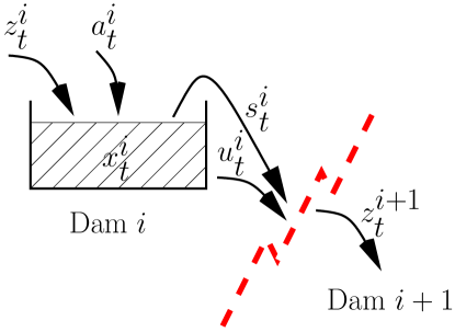
Figure 5: Decomposition by dam.

4.1.1 DADP implementation

The DADP method consists in choosing a multiplier process ${\boldsymbol{Y}}$ and then replacing the coupling constraints by their conditional expectations with respect to ${\boldsymbol{Y}}_{t}$. Here we adopt the choice ${\boldsymbol{Y}}_{t}=0$ (minimal information), so that Constraints (13) are replaced in the approximated problem by their expectations:

$$\mathbb{E}\big{(}{\boldsymbol{Z}}_{t}^{i+1}-g_{t}^{i}({\boldsymbol{X}}_{t}^{i},{\boldsymbol{U}}_{t}^{i},{\boldsymbol{W}}_{t}^{i},{\boldsymbol{Z}}_{t}^{i})\big{)}=0\;.$$ (14)

The expression of Subproblem (6) attached to dam $i$ reads

$$\max_{{\boldsymbol{U}}^{i},{\boldsymbol{Z}}^{i},{\boldsymbol{X}}^{i}}\quad \mathbb{E}\bigg{(}\sum_{t=0}^{T-1}\Big{(}L_{t}^{i}\big{(}{\boldsymbol{X}}_{t}^{i},{\boldsymbol{U}}_{t}^{i},{\boldsymbol{W}}_{t}^{i},{\boldsymbol{Z}}_{t}^{i}\big{)}\;+\;\mathbb{E}\big{(}{\boldsymbol{\Lambda}}_{t}^{i,(k)}\big{)}\cdot{\boldsymbol{Z}}_{t}^{i}$$ (15a)

$$\qquad-\;\mathbb{E}\big{(}{\boldsymbol{\Lambda}}_{t}^{i+1,(k)}\big{)}\cdot g_{t}^{i}\big{(}{\boldsymbol{X}}_{t}^{i},{\boldsymbol{U}}_{t}^{i},{\boldsymbol{W}}_{t}^{i},{\boldsymbol{Z}}_{t}^{i}\big{)}\Big{)}+K^{i}\big{(}{\boldsymbol{X}}_{T}^{i}\big{)}\bigg{)}\;,\qquad\qquad$$ (15b)

$$s.t.\qquad {\boldsymbol{X}}^{i}_{t+1}=f^{i}_{t}({\boldsymbol{X}}^{i}_{t},{\boldsymbol{U}}^{i}_{t},{\boldsymbol{W}}_{t})\;,\qquad{\boldsymbol{X}}^{i}_{0}\quad\text{given}$$ (15c)

$${\boldsymbol{U}}^{i}_{t}\;\;\>\preceq\sigma({\boldsymbol{W}}_{0},\ldots,{\boldsymbol{W}}_{t})\;.$$ (15d)

Because of the crude relaxation due to a constant ${\boldsymbol{Y}}_{t}^{i}$, the multipliers ${\boldsymbol{\Lambda}}_{t}^{i,(k)}$ appear only in the subproblems by means of their expectations $\mathbb{E}\big{(}{\boldsymbol{\Lambda}}_{t}^{i,(k)}\big{)}$, so that all subproblems involve a $1$-dimensional state variable, that is, the dam stock ${\boldsymbol{X}}^{i}_{t}$, and hence are easily solvable by Dynamic Programming.

We denote by $\big{(}{\boldsymbol{U}}^{i,(k)},{\boldsymbol{Z}}^{i,(k)},{\boldsymbol{X}}^{i,(k)}\big{)}$ the optimal solution of each subproblem $i$, and by $V_{t}^{i,(k)}(x^{i})$the Bellman function obtained for each dam $i$ at time $t$.

With the choice of constant information variables ${\boldsymbol{Y}}_{t}^{i}$, the coordination update step (11) reduces to

$$\mathbb{E}\big{(}{\boldsymbol{\Lambda}}_{t}^{i,(k+1)}\big{)}=\mathbb{E}\big{(}{\boldsymbol{\Lambda}}_{t}^{i,(k)}\big{)}+\rho_{t}\mathbb{E}\Big{(}{\boldsymbol{Z}}^{i+1,(k)}_{t}-g_{t}^{i}\big{(}{\boldsymbol{X}}^{i,(k)}_{t},{\boldsymbol{U}}^{i,(k)}_{t},{\boldsymbol{W}}_{t}^{i},{\boldsymbol{Z}}^{i,(k)}_{t}\big{)}\Big{)}\;,$$ (16)

that is, a collection of deterministic equations involving the expectation of (13) which is easily computable by a Monte Carlo approach.

Assume that DADP converges, leading to optimal Bellman functions $V_{t}^{i,\infty}$ and to optimal solutions $\big{(}{\boldsymbol{U}}^{i,\infty},{\boldsymbol{Z}}^{i,\infty},{\boldsymbol{X}}^{i,\infty}\big{)}$. We know that the initial almost-sure coupling constraints are not satisfied. To recover admissibility, the heuristic rule proposed at §3.3 consists in forming the global approximated Bellman $V_{t}^{\infty}$ functions as

$$V_{t}^{\infty}\big{(}x^{1},\ldots,x^{N}\big{)}=\sum_{i=1}^{N}V_{t}^{i,\infty}\big{(}x^{i}\big{)}\;,$$

and then computing, at any time $t$ and for any pair $(x_{t},w_{t})$, a control satisfying all the constraints of Problem (1) by solving the following one-step DP problem:

$$\max_{(u^{1},\ldots,u^{N})}\;\; \sum_{i=1}^{N}L_{t}^{i}\big{(}x^{i},u^{i},w_{t}^{i},z^{i}\big{)}+V_{t+1}^{\infty}\big{(}x_{t+1}^{1},\ldots,x_{t+1}^{N}\big{)}\;,$$

$$s.t.\quad\;\; x_{t+1}^{i}=f_{t}^{i}\big{(}x^{i},u^{i},w_{t}^{i},z^{i}\big{)}\quad\forall i\;,$$

$$z^{i+1}=g_{t}^{i}(x^{i},u^{i},w_{t}^{i},z^{i})\quad\;\forall i\;.$$

4.1.2 Complete process

To summarize, the whole process for implementing DADP is as follows.

• Optimization stage

  • Apply the DADP algorithm, and obtain at convergence the local Bellman functions $V_{t}^{i,\infty}$.

  • Form the approximated global Bellman functions $V_{t}^{\infty}$.

• Simulation stage

  • Draw a large number of noise scenarios (Monte Carlo sampling).

  • Compute the control values along each scenario by solving the one-step DP problems involving the Bellman functions $V_{t}^{\infty}$’s, thus satisfying all the constraints of Problem (1) as explained in §3.3; these computations produce for each scenario a state and control trajectories, as well as a payoff.

  • Evaluate the quality of the solution: trajectories variability, payoff distribution and associated mean…

4.2 SDDP implementations

As will be explained in §4.3, the controls of the original problem are discrete, which is a priori a difficulty for SDDP implemetation.

We describe here the two implementations of SDDP that we use for numerical comparisons, that is, a classical version of SDDP in which the integrity constraints on the control variables are relaxed (continuous controls) in order to use standard quadratic programming, and a homemade discrete version of SDDP described later on.

4.2.1 Continuous version of SDDP

The continuous implementation $\mathrm{SDDP}_{\!\mathrm{c}}$ of SDDP relaxes the integrity constraints upon the control ${\boldsymbol{U}}$, and assume that for all time $t$ and all dam $i$

$$x_{t}^{i}\in[\underline{x}^{i},\;\overline{x}^{i}]\quad\quad u_{t}^{i}\in[\underline{u}^{i},\;\overline{u}^{i}]\;.$$ (17)

Furthermore, $\mathrm{SDDP}_{\!\mathrm{c}}$ considers that the spillage is a control variable, so as to render the dynamic linear. As the dynamic is linear and costs convex, we are in the standard framework of Stochastic Dual Dynamic Programming and the resolution converges asymptotically to the optimal solution of the relaxed problem Girardeau et al. [2015].

The whole process of $\mathrm{SDDP}_{\!\mathrm{c}}$ is as follows.

• Optimization stage. The implementation of $\mathrm{SDDP}_{\!\mathrm{c}}$ corresponds to the one described in Shapiro [2011], that is, the so-called DOASA implementation. Lower approximations of the Bellman functions $V_{t}$ are built iteratively. At iteration $k$, the procedure consists of two passes.

  • During the forward pass, we first sample a scenario of noise. We then simulate a stock trajectory by using the current approximation of the Bellman functions. This is done by successively solving one-step DP problem to determine the next stock value. Each of these one-step DP problems is in fact a continuous quadratic programming (QP) problem.

  • In the backward pass, duality theory allows to find subgradient of lower approximations of the Bellman functions. This subgradients are used to construct valid cut, that is hyperplanes that are lower that the Bellman functions. Those cuts are then added to the current approximations of Bellman functions.

• Simulation stage. The simulation stage is identical to the one described at §4.1.2: the controls are computed with a one-step DP problem using the approximation of the Bellman functions obtained by $\mathrm{SDDP}_{\!\mathrm{c}}$.

The continuous version $\mathrm{SDDP}_{\!\mathrm{c}}$ is implemented in Julia, with the package StochDynamicProgramming built on top of the JuMP package used as a modeller Dunning et al. [2015]. The QP problems are solved using CPLEX 12.5. Every 5 iterations, redundant cuts are removed thanks to the limited memory level-1 heuristic described in Guigues [2017]. Indeed, without cuts removal, the resolution of each QP becomes too slow as the number of cuts increase along iterations. The algorithm is stopped after a fixed number of iterations and the gap is estimated with Monte-Carlo as described in Shapiro [2011].

4.2.2 Discrete version of SDDP

In the discrete version of $\mathrm{SDDP}_{\!\mathrm{d}}$, the controls ${\boldsymbol{U}}$ are discrete variables which have the same constraints as in the original problem formulation. Some other works mixing SDDP and binary variables are described in Zou et al. [2016] The whole process of $\mathrm{SDDP}_{\!\mathrm{d}}$ is as follows.

• Optimization stage. The implementation of $\mathrm{SDDP}_{\!\mathrm{d}}$ corresponds to the one described for $\mathrm{SDDP}_{\!\mathrm{c}}$ that is, approximations of the Bellman functions $V_{t}$ by a set of cuts which are built iteratively. At iteration $k$, the procedure consists of two passes.

  • During the forward pass, we first sample a scenario of noise. We then simulate a stock trajectory by using the current approximation of the Bellman functions. This is done by successively solving one-step DP problem to determine the next stock. Each of these one-step DP problems is solved by enumerating all possible values of the discrete control. In order to take advantage of the threading facilities, we may treat multiple noise scenarios in parallel (8 scenarios in practice).

  • In the backward pass, the approximations of the Bellman functions are refined along the trajectories computed during the forward pass. For each new added state point we first solve a one-step DP problem to obtain a new Bellman value. Then we solve a family of one step DP problem using as state points the neighbors on the grid of the current state point. We are thus able to approximate a new cut at the current state point by approximating derivatives of the Bellman function by finite differences (we use centered finite differences for regular states and forward, backward differences for states at domain boundary).

• Simulation stage. The simulation stage is identical to the one described at §4.1.2: the controls are computed with a one-step DP problem using the approximation of the Bellman functions obtained by $\mathrm{SDDP}_{\!\mathrm{d}}$.

The algorithm is stopped after a fixed number of iterations (25 in our experiments). The number of added points at forward step as already explained was set to 8. During the iterations some cuts were dropped by only keeping the last 100 cuts obtained for each Bellman function.

4.3 Results obtained for academic valleys

We model a first collection of hydro valleys including from 4 to 12 dams, with arborescent geometries (see Figure 6).

         

4-Dams        6-Dams              8-Dams                            10-Dams

Figure 6: Some academic examples of hydro valleys.

The optimization problem is stated on a time horizon of one year, with a monthly time step ($T=12$). All the dams have more or less the same maximal volume. The maximal amount of turbinated water for each dam varies with the location of the dam in the valley (more capacity for a downstream dam than for an upstream dam), as well as the random inflows in a dam (more inflow for an upstream dam than for a downstream dam). We assume discrete probability laws with finite supports for the inflows, and we also assume that the available turbine controls are discrete, so that each dam is in fact modeled using a discrete Markov chain. These valleys do not correspond to realistic valleys, in the sense that a true valley incorporates dams with very heterogeneous sizes.

4.3.1 DADP convergence

Let us first detail the gradient method used for the update of the multipliers involved by DADP. Thanks to the choice of constant information variables, the gradient expression involved in the update formula (16) is an expectation:

$$\mathbb{E}\Big{(}{\boldsymbol{Z}}^{i+1,(k)}_{t}-g_{t}^{i}\big{(}{\boldsymbol{X}}^{i,(k)}_{t},{\boldsymbol{U}}^{i,(k)}_{t},{\boldsymbol{W}}_{t}^{i},{\boldsymbol{Z}}^{i,(k)}_{t}\big{)}\Big{)}\;.$$

This expectation can be approximated by a Monte Carlo approach. We draw a collection of scenarios of $\{{\boldsymbol{W}}_{t}\}$ and then compute at iteration $k$ of DADP the optimal solutions $\big{\{}{\boldsymbol{X}}^{i,(k)}_{t},{\boldsymbol{U}}^{i,(k)}_{t},{\boldsymbol{Z}}^{i,(k)}_{t}\big{\}}$ of Subproblem (15) along each scenario. We thus obtain realizations of $\big{(}{\boldsymbol{Z}}^{i+1,(k)}_{t}-g_{t}^{i}({\boldsymbol{X}}^{i,(k)}_{t},{\boldsymbol{U}}^{i,(k)}_{t},{\boldsymbol{W}}_{t}^{i},{\boldsymbol{Z}}^{i,(k)}_{t})\big{)}$, whose arithmetic mean gives the (approximated) gradient component at time $t$ for the coupling at dam $i+1$ . This gradient can be used either in the standard steepest descent method such as in (16), or in a more sophisticated algorithm such as the conjugate gradient or the quasi-Newton method. We use in our numerical experiments a solver (limited memory BFGS) of the MODULOPT library from INRIA Gilbert & Jonsson [2007]. For all the valleys we studied, the convergence was fast (around 100 iterations regardless of the problem size). Figure 7 represents the evolution of the multipliers of dam connections for the 4-Dams valley along the iterations of the algorithm.

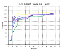
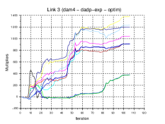
Figure 7: 4-Dams multipliers: dam1$\leftrightarrow$dam2 (left)  —  dam2$\leftrightarrow$dam3 (right)

4.3.2 Methods comparison

We solve Problem (1) for the first collection of academic valleys by 4 different methods:

1. the standard Dynamic Programming method (DP), if possible,

2. the continuous version of SDDP ($\mathrm{SDDP}_{\!\mathrm{c}}$) presented at §4.2.1,

3. the discrete version of SDDP ($\mathrm{SDDP}_{\!\mathrm{d}}$) presented at §4.2.2,

4. the DADP method (DADP).

All these methods produce Bellman functions (optimization stage described at §4.1.2), whose quality is evaluated by the simulation stage of §4.1.2. The obtained results are given in Table 1. The lines “CPU time” correspond to the time (in minute) needed to compute the Bellman functions (optimization stage), whereas the lines “value” indicate the cost obtained by Monte Carlo on the initial model (simulation stage, performed using a 100,000 scenarios sample, except for the 12-Dams valley for which a smaller sample set was used for computational time constraint). The comparisons between the different cost values for the same valley are thus relevant. For the two methods $\mathrm{SDDP}_{\!\mathrm{c}}$ and DADP, we also give the upper bound corresponding to the Bellman value obtained at the end of the optimization stage.

Valley	4-Dams	6-Dams	8-Dams	10-Dams	12-Dams
DP CPU time	$\mathit{1600}$’	$\sim\mathit{10^{8}}$’	$\sim\infty$	$\sim\infty$	$\sim\infty$
DP value	$3743$	N.A.	N.A.	N.A.	N.A.
$\mathrm{SDDP}_{\!\mathrm{d}}$ CPU time	$\mathit{2}$’	$\mathit{320}$’	$\mathit{2250}$’	$\mathit{133500}$’	$\sim\infty$
$\mathrm{SDDP}_{\!\mathrm{d}}$ value	$3737$	$7011$	$11750$	$16920$	N.A.
$\mathrm{SDDP}_{\!\mathrm{c}}$ CPU time	$\mathit{6}$’	$\mathit{10}$’	$\mathit{13}$’	$\mathit{50}$’	$\mathit{97}$’
$\mathrm{SDDP}_{\!\mathrm{c}}$ value	$3742$	$7027$	$11830$	$17070$	$\sim 17000$
$\mathrm{SDDP}_{\!\mathrm{c}}$ upper bound	$\mathit{3754}$	$\mathit{7050}$	$\mathit{11960}$	$\mathit{17260}$	$\mathit{19490}$
DADP CPU time	$\mathit{7}$’	$\mathit{12}$’	$\mathit{18}$’	$\mathit{24}$’	$\mathit{22}$’
DADP value	$3667$	$6816$	$11570$	$16760$	$\sim 17000$
DADP dual value	$\mathit{3996}$	$\mathit{7522}$	$\mathit{12450}$	$\mathit{17930}$	$\mathit{20480}$
Gap DADP/$\mathrm{SDDP}_{\!\mathrm{c}}$	$\mathbf{-2.0}$%	$\mathbf{-3.0}$%	$\mathbf{-2.2}$%	$\mathbf{-1.8}$%	$?$

Table 1: Results obtained by DP, $\mathrm{SDDP}_{\!\mathrm{d}}$, $\mathrm{SDDP}_{\!\mathrm{c}}$ and DADP

We first note that a direct use of DP is only possible for the 4-Dams valley: it corresponds to the well-known curse of dimensionality inherent to DP. The value given by DP is the true optimal cost value for the 4-Dams valley and can be used as the reference value. If we go on to the $\mathrm{SDDP}_{\!\mathrm{d}}$ method, we observe that it gives rather good results. The simulation cost obtained for the 4-Dams valley is very close to the one obtained by DP, which grounds the quality of the $\mathrm{SDDP}_{\!\mathrm{d}}$ method. But the method suffers from a curse of dimensionality associated to the control, in the sense that each optimization problem inside $\mathrm{SDDP}_{\!\mathrm{d}}$ has to enumerate all possible values of the discrete control, which becomes prohibitive for large valleys (number of possible controls for a single dam power number of dams). This explains why the method fails on the 12-Dams valley. Moreover, the $\mathrm{SDDP}_{\!\mathrm{d}}$ method does not provide any upper bound: the cuts are indeed computed by finite differences, so that we cannot guarantee that the cuts approximation is a lower approximation of the Bellman functions. The $\mathrm{SDDP}_{\!\mathrm{c}}$ method, although relying on the integrity constraints relaxation in the optimization stage (hence a not so tight upper bound), gives excellent results for the 4-Dams valley: we thus elect $\mathrm{SDDP}_{\!\mathrm{c}}$ as the reference method in order to evaluate the DADP method. Note that the CPU time remains reasonable, the optimization problems inside $\mathrm{SDDP}_{\!\mathrm{c}}$ corresponding to a continuous linear-quadratic formulation (here solved using the CPLEX commercial solver).

We now turn to the DADP method. We first notice that the upper bound given by the method is rather bad (as a consequence of solving a problem with relaxed coupling constraints in the optimization stage), but the values obtained in the simulation stage are correct compared to the ones given by $\mathrm{SDDP}_{\!\mathrm{c}}$ (as indicated by the last line of Table 1). The most noticeable point is that the CPU time needed for the optimization stage seems to grow more slowly for DADP than for $\mathrm{SDDP}_{\!\mathrm{c}}$. This aspect will be highlighted in §4.4.

Let us finally materialize more finely the difference in the results between $\mathrm{SDDP}_{\!\mathrm{c}}$ and DADP. Beyond average values given in Table 1, Figure 8 represents the payoff empirical probability laws (optimal cost over the time horizon), obtained by the simulation stage using 100,000 scenarios, for both $\mathrm{SDDP}_{\!\mathrm{c}}$ and DADP. We observe that, although the expectations are fairly close, the shapes of the two distributions differ significantly.

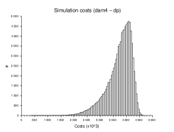
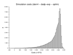
Figure 8: 4-Dams payoff distributions: $\mathrm{SDDP}_{\!\mathrm{c}}$ (left)  —  DADP (right)

4.4 Challenging the curse of dimensionality

The experiments made in §4.3 seem to indicate that DADP is less sensitive to the size of the valley than the $\mathrm{SDDP}_{\!\mathrm{c}}$ method. In order to validate this observation, we design a new collection of academic hydro valleys incorporating from $14$ up to $30$ dams. It is of course no more possible to perform the simulation stage for these instances: the combinatorics induced by the set of possible values of the controls is too large to allow to simulate the valley behavior along a large set of scenarios. We thus limit ourselves to the computation of the Bellman functions (optimization stage). The corresponding results are reported in Table 2.

Valley	14-Dams	18-Dams	20-Dams	25-Dams	30-Dams
$\mathrm{SDDP}_{\!\mathrm{c}}$ CPU time	$\mathit{210}$’	$\mathit{585}$’	$\mathit{970}$’	$\mathit{1560}$’	$\mathit{2750}$’
DADP CPU time	$\mathit{40}$’	$\mathit{50}$’	$\mathit{75}$’	$\mathit{140}$’	$\mathit{150}$’

Table 2: $\mathrm{SDDP}_{\!\mathrm{c}}$ and DADP comparison for large academic valleys

It appears that the CPU time required for the DADP method grows linearly with the number of dams, while the growth rate of $\mathrm{SDDP}_{\!\mathrm{c}}$ is more or less exponential. Figure 9 shows how the CPU time varies for the four methods. As expected, DP is only implementable for small instances, say up to $5$ dams. $\mathrm{SDDP}_{\!\mathrm{d}}$ allows to go a step further, but is limited by the combinatorial nature of the discrete controls we are considering. Finally, the limits of $\mathrm{SDDP}_{\!\mathrm{c}}$ and DADP have not really be reached, but DADP displays a linear rate allowing to tackle instances of even greater size.

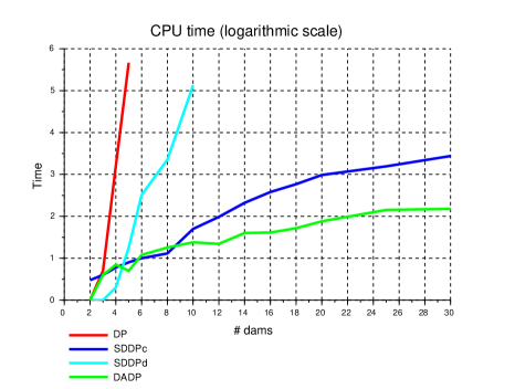
Figure 9: CPU time comparison

4.5 Results for two realistic valleys

We finally model two hydro valleys corresponding to existing systems in France, namely the Vicdessos valley and the Dordogne river (see Figure 10).

 

Vicdessos                                     Dordogne

Figure 10: Two realistic hydro valleys.

The optimization problem is posed again on a time horizon of one year, with a monthly time step. What mainly differ here from the academic examples used at §4.3 are the characteristics of the dams. For example, the Dordogne river valley encompasses large dams (as “Bort” whose capacity is say $400$) and small dams (as “Mareges” the capacity of which is equal to $35$, that is, ten times smaller). This heterogeneity induces numerical difficulties, as the fact to have at disposal a wide range of possible controls for the small downstream reservoirs, or the need to use a fine discretization for the state grid in DP-like methods. We again assume discrete probability laws with finite support for the inflows, and we also assume that the available turbine controls are discrete.

The comparison results of $\mathrm{SDDP}_{\!\mathrm{c}}$ and DADP are given in Table 3.

Valley	Vicdessos	Dordogne
$\mathrm{SDDP}_{\!\mathrm{d}}$ CPU time	$\mathit{90}$’	$\mathit{86000}$’
$\mathrm{SDDP}_{\!\mathrm{d}}$ value	$2234$	$21910$
$\mathrm{SDDP}_{\!\mathrm{d}}$ upper bound	$\mathit{2195}$	$\mathit{21370}$
$\mathrm{SDDP}_{\!\mathrm{c}}$ CPU time	$\mathit{9}$’	$\mathit{17}$’
$\mathrm{SDDP}_{\!\mathrm{c}}$ value	$2244$	$22150$
$\mathrm{SDDP}_{\!\mathrm{c}}$ upper bound	$\mathit{2258}$	$\mathit{22310}$
DADP CPU time	$\mathit{9}$’	$\mathit{210}$’
DADP value	$2238$	$21650$
DADP dual value	$\mathit{2286}$	$\mathit{22990}$
Gap DADP/$\mathrm{SDDP}_{\!\mathrm{c}}$	$\mathbf{-0.3}$%	$\mathbf{-2.2}$%

Table 3: Results obtained by $\mathrm{SDDP}_{\!\mathrm{c}}$, $\mathrm{SDDP}_{\!\mathrm{d}}$ and DADP

As for the academic examples, $\mathrm{SDDP}_{\!\mathrm{c}}$ displays the best results and is therefore used as the reference. The large number of possible discrete controls heavily penalizes the $\mathrm{SDDP}_{\!\mathrm{d}}$ methods. We also observe that this large combinatorics is a difficulty even for DADP, although the resolution is done dam by dam. Finally, the gap between $\mathrm{SDDP}_{\!\mathrm{c}}$ and DADP remains limited.

5 Conclusion

In this article, we have depicted a method called DADP which allows to tackle large-scale stochastic optimal control problems in discrete time, such as the ones found in the field of energy management. We have mainly presented the practical aspects of the method, without deepening in the theoretical issues arising in the foundations of the method. A lot of numerical experiments have been presented on hydro valley problems (“chained models”), which complements the ones already made on unit commitment problems (“flower models”) Barty et al. [2010b, a]. The main conclusions are that DADP, on the one hand converges fast, and on the other hand gives near-optimal results even when using a “crude” relaxation (here a constant information process ${\boldsymbol{Y}}$). More precisely, DADP allows to deal with optimization problems that are out of the scope of standard Dynamic Programming, and beats SDDP for very large hydro valleys in terms of CPU time. We thus hope to be able to implement DADP for very large stochastic optimal control problems such as the ones encountered in smart management of urban districts, involving hundreds of houses and thus hundred of dynamic variables.

The main perspectives that we see beyond this study are to extend it in two directions. The first direction consists in implementing the DADP method for general spatial structures (not only “flower models” or “chain model”, but “smart-grid models” involving a planar graph). The second direction is to implement more sophisticated decomposition methods than price decomposition. On the one hand we want to make use of decomposition schemes such that resource allocation or interaction prediction principle Cohen [1978]. On the other hand we want to use augmented Lagrangian based methods such as alternating direction method of multiplier (ADMM) and proximal decomposition algorithm (PDA) for decomposition in order to obtain the nice convergence properties of this kind of methods (see Lenoir & Mahey [2017] for a survey).

Finally, let us mention that a theoretical work has begun in order to provide foundations of the method Leclère [2014], Leclere [2013] it includes conditions for existence of a multiplier in the $L^{1}$ space when the optimization problem is posed in $L^{\infty}$ and conditions for convergence of the Uzawa algorithm in $L^{\infty}$. A lot of work remains to be done on these questions, mainly to relax the continuity assumption in order to be able to deal with extended functions, and to obtain more general assumptions ensuring the convergence of Uzawa algorithm.

Acknowledgments

This research benefited from the support of the FMJH “Program Gaspard Monge for optimization and operations research”, and from the support from EDF.

References

References

- Alais [2013] Alais, J.-C. (2013). Risque et optimisation pour le management d’énergies. Thèse de doctorat Université Paris-Est.
- Bacaud et al. [2001] Bacaud, L., Lemaréchal, C., Renaud, A., & Sagastizábal, C. A. (2001). Bundle methods in stochastic optimal power management: A disaggregated approach using preconditioner. Computational Optimization and Applications, 20, 227–244.
- Barty et al. [2010a] Barty, K., Carpentier, P., Cohen, G., & Girardeau, P. (2010a). Price decomposition in large-scale stochastic optimal control. ArXiv:1012.2092.
- Barty et al. [2010b] Barty, K., Carpentier, P., & Girardeau, P. (2010b). Decomposition of large-scale stochastic optimal control problems. RAIRO Operations Research, 44, 167–183.
- Barty et al. [2009] Barty, K., Roy, J.-S., & Strugarek, C. (2009). A stochastic gradient type algorithm for closed-loop problems. Mathematical Programming, Series A, 119, 51–78.
- Bellman [1957] Bellman, R. (1957). Dynamic Programming. New Jersey: Princeton University Press.
- Bellman & Dreyfus [1959] Bellman, R., & Dreyfus, S. E. (1959). Functional approximations and dynamic programming. Math tables and other aides to computation, 13, 247–251.
- Bertsekas [2000] Bertsekas, D. P. (2000). Dynamic Programming and Optimal Control. (2nd ed.). Athena Scientific.
- Bertsekas [2012] Bertsekas, D. P. (2012). Dynamic Programming and Optimal Control: Approximate Dynamic Programming. (4th ed.). Athena Scientific.
- Bertsekas & Tsitsiklis [1996] Bertsekas, D. P., & Tsitsiklis, J. N. (1996). Neuro-Dynamic Programming. Athena Scientific.
- Carpentier et al. [2015] Carpentier, P., Chancelier, J.-P., Cohen, G., & De Lara, M. (2015). Stochastic Multi-Stage Optimization volume 75 of Probability Theory and Stochastic Modelling. Springer International Publishing.
- Carpentier et al. [1996] Carpentier, P., Cohen, C., Culioli, J.-C., & Renaud, A. (1996). Stochastic optimization of unit commitment: a new decomposition framework. IEEE Transactions on Power Systems, 11, 1067–1073.
- Cohen [1978] Cohen, G. (1978). Optimization by Decomposition and Coordination: A Unified Approach. IEEE Transactions on Automatic Control, 23, 222–232.
- Cohen [1980] Cohen, G. (1980). Auxiliary Problem Principle and decomposition of optimization problems. Journal of Optimization Theory and Applications, 32, 277–305.
- Cohen & Culioli [1990] Cohen, G., & Culioli, J.-C. (1990). Decomposition Coordination Algorithms for Stochastic Optimization. SIAM J. Control Optimization, 28, 1372–1403.
- Dellacherie & Meyer [1975] Dellacherie, C., & Meyer, P. A. (1975). Probabilités et potentiel. Paris: Hermann.
- Dunning et al. [2015] Dunning, I., Huchette, J., & Lubin, M. (2015). JuMP: A modeling language for mathematical optimization. arXiv:1508.01982 [math.OC], .
- Ekeland & Temam [1999] Ekeland, I., & Temam, R. (1999). Convex Analysis and Variational Problems volume 28 of Classics in Applied Mathematics. SIAM.
- Gilbert & Jonsson [2007] Gilbert, J. C., & Jonsson, X. (2007). Libopt–an environment for testing solvers on heterogeneous collections of problems. Submitted to ACM Transactions on Mathematical Software, .
- Girardeau [2010] Girardeau, P. (2010). Résolution de grands problèmes en optimisation stochastique dynamique. Thèse de doctorat Université Paris-Est.
- Girardeau et al. [2015] Girardeau, P., Leclere, V., & Philpott, A. B. (2015). On the convergence of decomposition methods for multistage stochastic convex programs. Mathematics of Operations Research, 40, 130–145.
- Guigues [2017] Guigues, V. (2017). Dual dynamic programing with cut selection: Convergence proof and numerical experiments. European Journal of Operational Research, 258, 47–57.
- Heitsch & Römisch [2009] Heitsch, H., & Römisch, W. (2009). Scenario tree modelling for multistage stochastic programs. Mathematical Programming, 118, 371–406.
- Heitsch et al. [2006] Heitsch, H., Römisch, W., & Strugarek, C. (2006). Stability of multistage stochastic programs. SIAM Journal on Optimization, 17, 511–525.
- Leclere [2013] Leclere, V. (2013). Epiconvergence of relaxed stochastic optimization problem. hal-00848275, .
- Leclère [2014] Leclère, V. (2014). Contributions aux méthodes de décomposition en optimisation stochastique. Thèse de doctorat Université Paris-Est.
- Lenoir & Mahey [2017] Lenoir, A., & Mahey, P. (2017). A survey on operator splitting and decomposition of convex programs. RAIRO Operations Research, 51, 17–41.
- Maceira & Damazio [2006] Maceira, M. E. P., & Damazio, J. M. (2006). Use of par(p) model in the stochastic dual dynamic programming optimization scheme used used in the operation planning of the brazilian hydropower system. Probability in the Engineering and Informational Sciences, 20, 143–156.
- de Matos et al. [2015] de Matos, V. L., Philpott, A. B., & Finardi, E. C. (2015). Improving the performance of stochastic dual dynamic programming. Journal of Computational and Applied Mathematics, 290, 196–208.
- Pereira & Pinto [1991] Pereira, M. V. F., & Pinto, L. M. V. G. (1991). Multi-stage stochastic optimization applied to energy planning. Mathematical Programming, 52, 359–375.
- Pflug & Pichler [2014] Pflug, G. C., & Pichler, A. (2014). Multistage Stochastic Optimization. Springer.
- Philpott & Guan [2008] Philpott, A. B., & Guan, Z. (2008). On the convergence of stochastic dual dynamic programming and related methods. Operations Reseach Letters, 36, 450–455.
- Powell [2011] Powell, W. B. (2011). Approximate Dynamic Programming: Solving the Curses of Dimensionality volume 842. John Wiley & Sons.
- Puterman [1994] Puterman, M. (1994). Markov Decision Processes: Discrete Stochastic Dynamic Programming. New York, NY: John Wiley and Sons.
- Rockafellar [1968] Rockafellar, R. T. (1968). Integrals which are convex functionals. Pacific Journal of Mathematics, 24, 525–539.
- Rockafellar [1971] Rockafellar, R. T. (1971). Integrals which are convex functionals, ii. Pacific Journal of Mathematics, 39, 439–469.
- Rockafellar & Wets [1991] Rockafellar, R. T., & Wets, R. J.-B. (1991). Scenarios and policy aggregation in optimization under uncertainty. Math. Oper. Res., 16, 119–147.
- Ruszczyński [1997] Ruszczyński, A. (1997). Decomposition methods in stochastic programming. Mathematical programming, 79, 333–353.
- Ruszczyński & Shapiro [2003] Ruszczyński, A., & Shapiro, A. (Eds.) (2003). Stochastic Programming volume 10 of Handbooks in Operations Research and Management Science. Elsevier.
- Shapiro [2006] Shapiro, A. (2006). On complexity of multistage stochastic programs. Operations Research Letters, 34, 1–8.
- Shapiro [2011] Shapiro, A. (2011). Analysis of Stochastic Dual Dynamic Programming Method. European Journal of Operational Research, 209, 63–72.
- Shapiro et al. [2009] Shapiro, A., Dentcheva, D., & Ruszczyński, A. (2009). Lectures on Stochastic Programming. Society for Industrial and Applied Mathematics, Philadelphia.
- Strugarek [2006] Strugarek, C. (2006). Approches variationnelles et autres contributions en optimisation stochastique. Ph.D. thesis École Nationale des Ponts et Chaussées.
- Takriti et al. [1996] Takriti, S., Birge, J. R., & Long, E. (1996). A stochastic model for the unit commitment problem. IEEE Transactions on Power Systems, 11, 1497–1508.
- Tsitsiklis & Van Roy [1996] Tsitsiklis, J. N., & Van Roy, B. (1996). Feature-based methods for large-scale dynamic programming. Machine Learning, 22, 59–94.
- Van Slyke & Wets [1969] Van Slyke, R. M., & Wets, R. (1969). L-shaped linear programs with applications to optimal control and stochastic programming. SIAM Journal on Applied Mathematics, 17, 638–663.
- Vezolle et al. [2009] Vezolle, P., Vialle, S., & Warin, X. (2009). Large Scale Experiment and Optimization of a Distributed Stochastic Control Algorithm. Application to Energy Management Problems. In International workshop on Large-Scale Parallel Processing (LSPP 2009). Rome, Italy.
- Zou et al. [2016] Zou, J., Ahmed, S., & Sun, X. A. (2016). Nested decomposition of multistage stochastic integer programs with binary state variables. Optimization Online, 5436.