Efficient covariance approximations for large sparse precision matrices

Abstract.

The use of sparse precision (inverse covariance) matrices has become popular because they allow for efficient algorithms for joint inference in high-dimensional models. Many applications require the computation of certain elements of the covariance matrix, such as the marginal variances, which may be non-trivial to obtain when the dimension is large. This paper introduces a fast Rao-Blackwellized Monte Carlo sampling-based method for efficiently approximating selected elements of the covariance matrix. The variance and confidence bounds of the approximations can be precisely estimated without additional computational costs. Furthermore, a method that iterates over subdomains is introduced, and is shown to additionally reduce the approximation errors to practically negligible levels in an application on functional magnetic resonance imaging data. Both methods have low memory requirements, which is typically the bottleneck for competing direct methods.

1. Introduction

We consider the problem of computing selected elements of the covariance matrix $\boldsymbol{\Sigma}$ of a multivariate normal distribution, which is parameterized using the precision matrix $\mathbf{Q}=\boldsymbol{\Sigma}^{-1}$. Specifying models with the precision matrix rather than the covariance matrix is useful (or even necessary) in many high-dimensional applications, since it allows for a sparse representation, typically leading to smaller time and memory complexity. Their use has a long history in spatial statistics (Besag,, 1974; Rue and Held,, 2005), image processing (Jeng and Woods,, 1991), and probabilistic graphical models (Lauritzen,, 1996; Malioutov et al.,, 2006).

The desire to compute certain elements of the covariance matrix arises in many applications. If $\mathbf{Q}$ is the posterior precision matrix in a Bayesian analysis, then the diagonal of $\boldsymbol{\Sigma}$ contains the posterior marginal variances, which are often presented as a measure of marginal uncertainty. Furthermore, joint posterior statistics of larger subdomains will normally also require the computation of certain off-diagonal elements of $\boldsymbol{\Sigma}$. This is for example the case when computing the posterior probability of exceeding a threshold in a specific subdomain, which is the topic of Bolin and Lindgren, (2015), and which has applications in temperature modeling (Furrer et al.,, 2007), astrophysics (Beaky et al.,, 1992) and brain imaging (Sidén et al.,, 2017). Computing submatrices of $\boldsymbol{\Sigma}$ is also needed for characterizing the uncertainty of a robot’s location in an unknown environment (Thrun et al.,, 2005).

Even though $\mathbf{Q}$ is sparse, $\boldsymbol{\Sigma}$ is dense in general, and the naive direct inversion $\boldsymbol{\Sigma}=\mathbf{Q}^{-1}$ is not an option even for relatively small dimensions. Fortunately, as described in the next section, when only selected elements of $\boldsymbol{\Sigma}$ are required, a number of less computationally intensive exact methods exist in the literature. However, for modern applications the dimensionality of the problem can be too large even for these methods to be computationally feasible. Usually the bottleneck is in the memory requirements, even though computation times can also be unpleasantly long. This often leads to investigators choosing to perform their analyses on smaller subsets of the data independently or at a lower resolution than desired. Another situation in which the memory is normally a limitation is when performing these operations on robots or other embedded systems.

In this paper, we develop a fast Rao-Blackwellized Monte Carlo sampling-based method for approximating the elements of the covariance matrix, and show its efficiency compared to existing sampling-based methods. We further show that the variances and confidence bounds of the approximations can be cheaply computed by inserting the approximated values into analytical expressions. In addition, a second, more exact method is developed, which by using the estimates from the first method as starting values and by iterating over subdomains, produces estimates with negligible error in practice. Both methods build on decompositions of the domain on which the GMRF is defined, into subdomains that can be processed nearly independently, leading to low memory requirements and algorithms that are easily parallelized. We evaluate the methods on precision matrices from theoretical models and on a posterior precision matrix from a functional magnetic resonance imaging (fMRI) experiment.

The outline of the article follows. In the next section, we give a theoretical background to the problem and an overview of existing methods and their limitations. We present the developed methods in Section 3 and numerically evaluate their performance in Section 4. Section 5 is a discussion and Section 6 concludes. A Matlab implementation of the methods in the article is available at https://github.com/psiden/CovApprox.

2. Background and literature review

We assume that $\mathbf{x}\sim\mathsf{N}\left(\boldsymbol{\mu},\mathbf{Q}^{-1}\right)$ is an $N$-dimensional multivariate normally distributed random variable, and that $\mathbf{Q}$ is a sparse symmetric positive definite precision matrix. Such a distribution is commonly referred to as a Gaussian Markov random field (GMRF) (Rue and Held,, 2005) and the sparsity pattern of $\mathbf{Q}$ has a natural interpretation in that an element $Q_{i,j}$ is zero if and only if the corresponding elements $x_{i}$ and $x_{j}$ are conditionally independent given all other elements. We assume, for simplicity and without loss of generality, that $\boldsymbol{\mu}=\mathbf{0}$.

Selected inversion refers to the computation of $\boldsymbol{\Sigma}_{\mathcal{S}}$ for some set of indices
$\mathcal{S}\subset\left\{\left(i,j\right);1\leq i,j\leq N\right\}$, with $\left|\mathcal{S}\right|\ll N^{2}$, for example $\mathcal{S}=\mathcal{S}_{I}=\left\{\left(i,j\right);i=j\right\}$ gives the diagonal. We will also use the (slightly abusive) notation $\boldsymbol{\sigma}^{\mathbf{2}}=\left[\sigma_{1}^{2},\ldots,\sigma_{N}^{2}\right]=\boldsymbol{\Sigma}_{\mathcal{S}_{I}},$ to denote the marginal variances. Other commonly appearing examples of index sets for selected inversion are $\mathcal{S}_{\mathbf{aa}^{T}}=\left\{\left(i,j\right);a_{i}\neq 0,a_{j}\neq 0\right\}$, for some sparse column vector $\mathbf{a}$, and $\mathcal{S}_{\mathbf{R}}=\left\{\left(i,j\right);R_{ij}\neq 0\right\}$, for some sparse symmetric matrix $\mathbf{R}$. The first can be used to compute $Var\left(\mathbf{a}^{T}\text{{x}}\right)=\mathbf{a}^{T}\boldsymbol{\Sigma}\mathbf{a}=\sum_{i,j}a_{i}a_{j}\Sigma_{i,j}$, and the second when computing $tr\left(\mathbf{R}\boldsymbol{\Sigma}\right)=\sum_{i,j}R_{i,j}\Sigma_{i,j}$, which is commonly needed in some inference methods such as the expectation maximization (EM) algorithm (Bolin et al.,, 2009) and variational Bayes (VB) (Rue et al.,, 2009). Depending on $\mathcal{S}$ and the sparsity pattern of $\mathbf{Q}$, different methods for selected inversion might be preferable.

A naive method for selected inversion that always works in theory for any $\mathcal{S}$, is of course to completely compute $\boldsymbol{\Sigma}=\mathbf{Q}^{-1}$ using a standard method, for example Gaussian elimination, and then extract $\boldsymbol{\Sigma}_{\mathcal{S}}$. Such a method is of time complexity $O\left(N^{3}\right)$ and memory complexity $O$$\left(N^{2}\right)$ which is prohibitive even for rather small values of $N$. By exploiting the sparsity patterns in $\mathcal{S}$ and $\mathbf{Q}$, this complexity can often be greatly reduced.

Another trivial idea for selected inversion is that column $j$ of $\boldsymbol{\Sigma}$ can be computed by solving $\mathbf{Qz}=\mathbf{e}_{j}$ for $\mathbf{z}$, where $\mathbf{e}_{j}$ is the $j$th column of the $N\times N$ identity matrix. The computational cost of this operation may be high for large $N$, but can be greatly reduced by using iterative methods such as the preconditioned conjugate gradient (PCG) algorithm (Manteuffel,, 1980; Barrett et al.,, 1994). This method produces an approximate solution by iteratively minimizing the relative residual $\left\|\mathbf{Qz}-\mathbf{e}_{j}\right\|/\left\|\mathbf{e}_{j}\right\|$ until it decreases below some specified level $\delta$, that can be set arbitrarily low. The time complexity of iterative methods can be nearly linear in $N$ for diagonally dominant matrices $\mathbf{Q}$, which are matrices $Q_{i,i}>\sum_{i\neq j}\left|Q_{i,j}\right|$ for all $i$ (Spielman and Teng,, 2004). However, in general PCG has complexity $O\left(m\sqrt{\kappa}\right)$, where $m$ is the number of nonzero elements in $\mathbf{Q}$ and $\kappa$ is its condition number. This for example gives complexity $O\left(N^{1+1/d}\right)$ if $\mathbf{Q}$ is obtained from a finite element approximation of a second-order elliptic boundary value problem posed on a $d$-dimensional domain (Shewchuk,, 1994). This strategy will therefore have at least quadratic complexity when the selected elements are in all columns (for example when computing $\boldsymbol{\Sigma}_{\mathcal{S}_{I}}$), which will often be too costly, but it can be useful when the number of selected elements is small.

Direct methods for selected inversion usually rely on first computing the Cholesky decomposition $\mathbf{LL}^{T}=\mathbf{Q}$, where $\mathbf{L}$ is lower triangular. This operation also takes $O\left(N^{3}\right)$ time in general, but by using reordering techniques, for example approximate minimum degree reordering (Amestoy et al.,, 1996), it can generally be reduced to $O\left(N^{3/2}\right)$ for 2D problems and $O\left(N^{2}\right)$ for 3D problems (Rue and Held,, 2005). It is, however, the memory requirements that normally make these methods unfeasible (Aune et al.,, 2014). The complexity mainly depends on the sparsity pattern of $\mathbf{L}$, whose dependency on $\mathbf{Q}$ is nicely explained from a graph theoretical point of view in Vandenberghe and Andersen, (2014). We denote the index set of the symbolic Cholesky factorization by $\mathcal{L}_{\mathbf{Q}}$ (edges in the chordal extension of the graph corresponding to $\mathbf{Q}$), which has the property that $\mathcal{L}_{\mathbf{Q}}\supseteq\mathcal{S}_{\mathbf{L}+\mathbf{L}^{T}}\cup\mathcal{S}_{\mathbf{Q}}$, but in most cases $\mathcal{L}_{\mathbf{Q}}=\mathcal{S}_{\mathbf{L}+\mathbf{L}^{T}}$. Largely speaking, the complexity is low whenever the fill-in $\mathcal{L}_{\mathbf{Q}}\setminus\mathcal{S}_{\mathbf{Q}}$ is small.

The probably oldest idea for direct selected inversion, referred to as the Takahashi equations (Takahashi et al.,, 1973; Erisman and Tinney,, 1975), is nicely presented and compactly derived in Rue and Martino, (2007). A statistical derivation in the same article begins by noting that

$$x_{i}|\mathbf{x}_{i+1:N}\sim\mathsf{N}\left(-\frac{1}{L_{i,i}}\sum_{k=i+1}^{N}L_{k,i}x_{k},1/L_{i,i}^{2}\right),$$ (2.1)

which provides a sequential representation of the GMRF. For $j\geq i$ it is straightforward to derive that

$$\Sigma_{ij} = E\left(x_{i}x_{j}\right)=E\left[E\left(x_{i}x_{j}|\mathbf{x}_{i+1:N}\right)\right]=\frac{\mathbb{1}_{\left\{i=j\right\}}}{L_{i,i}^{2}}-\frac{1}{L_{i,i}}\sum_{k=i+1}^{N}L_{k,i}\Sigma_{k,j}.$$ (2.2)

By iterating backwards, for $i=N,\ldots,1$ and for each $i,$ $j=N,\ldots,i$, one can compute the full $\boldsymbol{\Sigma}$ recursively. Furthermore, because of the sparsity structure of $\mathbf{L}$, many terms of the sum in Eq. (2.2) will be zero, and the authors show that it is enough to compute $\Sigma_{ij}$ for iterations where $\left(i,j\right)\in\mathcal{L}_{\mathbf{Q}}$ and to sum over indices where $\left(k,i\right)\in\mathcal{L}_{\mathbf{Q}}$ for the computations to be correct for all of $\boldsymbol{\Sigma}_{\mathcal{L}_{\mathbf{Q}}}$. Therefore, if the selected elements $\mathcal{S}$ form a subset of $\mathcal{L}_{\mathbf{Q}}$, which is true for example for $\mathcal{S}_{\mathbf{Q}}$ and $\mathcal{S}_{I}$, this method is sufficient for computing the selected inverse. If $\mathcal{S}=\mathcal{S}_{\mathbf{R}}$ is not a subset of $\mathcal{L}_{\mathbf{Q}}$, then one could easily show that it will be sufficient to iterate over the Takahashi equations for indices in $\mathcal{L}_{\left|\mathbf{Q}\right|+\left|\mathbf{R}\right|}$ instead, by applying Theorem 1 in Rue and Martino, (2007) on the graph corresponding to $\left|\mathbf{Q}\right|+\left|\mathbf{R}\right|$. The time complexity of solving the Takahashi equations is similar that of Cholesky factorization as illustrated in Vandenberghe and Andersen, (2014, Fig. 9.5).

In the literature on numerical linear algebra, some effort has in recent years been devoted to improving this and similar direct methods (Li et al.,, 2008; Lin et al., 2011a, ; Lin et al., 2011b, ; Rouet,, 2012; Amestoy et al.,, 2012; Vandenberghe and Andersen,, 2014; Amestoy et al.,, 2015; Xia et al.,, 2015; Jacquelin et al.,, 2015). The new techniques use various reorderings, multifrontal and supernodal strategies, cleverly adapted to the sparsity structure in $\mathbf{Q}$, in order to distribute computations and storage in efficient ways, see Vandenberghe and Andersen, (2014) for an in depth explanation. For problems of moderate size, these methods are very competitive, but will always have memory limitations for problems of higher dimensionality.

In the field of probabilistic graphical models, belief propagation (BP) and loopy belief propagation (LBP) (Pearl,, 1988; Malioutov et al.,, 2006) are well-known algorithms for inferring the marginal distributions of the nodes of a graphical model, by iteratively passing messages between neighboring nodes using various message passing schemes. When applied to GMRFs, these algorithms compute the means and marginal variances of all nodes, resulting in the covariance matrix diagonal. In this case, each message passing step is related to computing the Schur complement $\boldsymbol{\Sigma}_{\mathcal{I},\mathcal{I}}=\left(\mathbf{Q}_{\mathcal{I},\mathcal{I}}-\mathbf{Q}_{\mathcal{I},\mathcal{I}^{c}}\mathbf{Q}_{\mathcal{I}^{c},\mathcal{I}^{c}}^{-1}\mathbf{Q}_{\mathcal{I}^{c},\mathcal{I}}\right)^{-1}$, applied to a single node, $\mathcal{I}=\left\{i\right\}$, see Malioutov et al., (2006) for details. Of course, $\mathbf{Q}_{\mathcal{I}^{c},\mathcal{I}^{c}}^{-1}$ is unavailable for large graphs, but an approximation, based on saved results from previous iterations of the algorithm, can be computed for elements corresponding to neighbors of node $i$. These are the only ones required due to the sparsity pattern of $\mathbf{Q}_{\mathcal{I},\mathcal{I}^{c}}$. If the graph is a tree, BP can be used to produce the exact marginal variances in a finite number of iterations. This largely corresponds to applying the Cholesky factorization and Takahashi equations in the case with no fill-in, which is also computationally cheap. In the common case that the graph is not a tree, LBP must be used, which is known to not converge for all models. Malioutov et al., (2006) show that a sufficient condition for the convergence of the means and variances is that the model is walk-summable, a property including for example models that have a diagonally dominant $\mathbf{Q}$. However, only the means, and not the variances, are guaranteed to converge to the true values, which together with the fact that many models are not walk-summable limits the use of these methods.

As a remedy, Liu et al., (2012) introduce a modified version named feedback message passing (FMP), that first removes a number of “feedback nodes” from the graph so that the remaining graph is cycle-free. BP is then used to get the exact solution for this graph, that can be passed back to the feedback nodes which in turn can now also get the correct variances computed. In a final step, information from the feedback nodes is used to compute the exact variances in the cycle-free part of the graph. The method is exact and bears resemblance with some of the methods from numerical linear algebra presented above, but also becomes computationally intractable as the problem, and in particular the number of required feedback nodes, becomes large. In addition, a separate, faster, approximate FMP method is developed, in which a smaller number of feedback nodes is selected so that the remaining graph is no longer cycle-free, but at least walk-summable or almost walk-summable. Approximate FMP is not exact, but is empirically shown to produce reasonable approximations of the variances on some small examples.

A number of papers look at sampling-based approaches for estimating the selected inverse. The idea in Bekas et al., (2007) origins from the paper by Hutchinson, (1990) and suggests estimating the matrix diagonal as

$$\hat{\boldsymbol{\sigma}}^{\mathbf{2}}=\left[\sum_{j=1}^{N_{s}}\mathbf{v}^{\left(j\right)}\odot\boldsymbol{\Sigma}\mathbf{v}^{\left(j\right)}\right]\oslash\left[\sum_{j=1}^{N_{s}}\mathbf{v}^{\left(j\right)}\odot\mathbf{v}^{\left(j\right)}\right],$$ (2.3)

where $\odot$ and $\oslash$ means component-wise multiplication and division of vectors respectively, where $\mathbf{v}^{\left(j\right)}$ is an $N$-dimensional random vector, for example a vector where each element independently has value $1$ or $-1$ with equal probability, and where $N_{s}$ is the number of sampled vectors. The method requires the computation of $\boldsymbol{\Sigma}\mathbf{v}^{\left(j\right)}$, which in our case can be done by solving $\mathbf{Q}\mathbf{z}=\mathbf{v}^{\left(j\right)}$ for $\mathbf{z}$, using PCG methods. The estimator in Eq. (2.3) is unbiased, and it is also exact if the rows ($i$ and $j$) of $\mathbf{V}_{s}=\left[\mathbf{v}^{\left(1\right)},\ldots,\mathbf{v}^{\left(N_{s}\right)}\right]$ are orthogonal for all $i$ and $j$ for which $\boldsymbol{\Sigma}_{i,j}\neq 0$. If $\boldsymbol{\Sigma}$ is dense, this condition implies that $N_{s}=N$ is required for exactness (for example by choosing $\mathbf{v}^{\left(j\right)}=\mathbf{e}_{j}$), which is not very helpful. However, this condition still motivates choosing the columns of $\mathbf{V}_{s}$ deterministically, such that the rows are non-orthogonal only for $i$ and $j$ such that $\boldsymbol{\Sigma}_{i,j}$ is small. By assuming that the off-diagonal elements of $\boldsymbol{\Sigma}$ decays with distance, Bekas et al., (2007) motivates selecting $\mathbf{V}_{s}$ as a Hadamard matrix to get a good approximation. The same sort of argument can be used to motivate selecting $\mathbf{v}_{j}$ as probing vectors (Tang and Saad,, 2012), but this requires first coloring the graph corresponding to $\mathbf{Q}^{p}$ for some suitable integer $p$. Malioutov et al., (2008) also use coloring to select the rows of $\mathbf{V}_{s}$ as orthogonal for nodes that are close, but in addition they provide a multiscale wavelet basis for $\mathbf{V}_{s}$, that works better for long-range correlation models and multiscale models.

Papandreou and Yuille, (2010) develop an algorithm for fast sampling from $\mathsf{N}\left(\mathbf{0},\mathbf{Q}^{-1}\right)$ when $\mathbf{Q}$ can be written as $\mathbf{G}^{T}\mathbf{G}+\mathbf{H}^{T}\mathbf{H}$, for some sparse matrices $\mathbf{G}$ and $\mathbf{H}$, which is a situation that often appears naturally when $\mathbf{Q}$ is a posterior precision matrix, see for example the models in Section 4. In these cases, a sample can be produced as $\mathbf{x}^{\left(j\right)}=\mathbf{Q}^{-1}\left(\mathbf{G}^{T}\mathbf{z}_{1}+\mathbf{H}^{T}\mathbf{z}_{2}\right)$, where $\mathbf{z}_{1}$ and $\mathbf{z}_{2}$ are standard normal i.i.d. sampled vectors of appropriate lengths. For efficiency, the PCG method can also here be used to solve the equation system with respect to $\mathbf{Q}$. A similar algorithm is provided by Bhattacharya et al., (2016) to sample from the conditional posterior in high-dimensional regression with Gaussian scale mixture priors. Given $N_{s}$ independent samples of $\mathbf{x}$, denoted $\mathbf{X}=\left[\mathbf{x}^{\left(1\right)},\ldots,\mathbf{x}^{\left(N_{s}\right)}\right]$, simple Monte Carlo (MC) estimators of $\boldsymbol{\Sigma}$ and $\sigma_{i}^{2}$ are

$$\hat{\boldsymbol{\Sigma}}_{MC}=\frac{1}{N_{s}}\sum_{j=1}^{N_{s}}\mathbf{x}^{\left(j\right)}\mathbf{x}^{\left(j\right)T}=\frac{1}{N_{s}}\mathbf{X}\mathbf{X}^{T},\,\,\,\,\,\,\,\text{$\sigma_{MC,i}^{2}=\frac{1}{N_{s}}\sum_{j=1}^{N_{s}}\left(x_{i}^{\left(j\right)}\right)^{2}$,}$$ (2.4)

which are further explored in Papandreou and Yuille, (2011). The estimators follow scaled Wishart and chi-squared distributions with $N_{s}$ degrees of freedom, $\hat{\boldsymbol{\Sigma}}_{MC}\sim\frac{1}{N_{s}}\mathsf{Wishart}\left(\boldsymbol{\Sigma},N_{s}\right)$ and $\hat{\sigma}_{MC,i}^{2}\sim\frac{\sigma_{i}^{2}}{N_{s}}\chi_{N_{s}}^{2}$, and are thus unbiased, see for example Mardia et al., (1979, Chapter 3). By defining the relative error with respect to the true marginal variances of the second estimator as $r_{MC,i}=\nicefrac{{\left(\hat{\sigma}_{MC,i}^{2}-\sigma_{i}^{2}\right)}}{{\sigma_{i}^{2}}}$ and the relative root-mean-square error (relative RMSE) as $RMSE_{MC,i}=\sqrt{E\left[r_{MC,i}^{2}\right]}$, the unbiasedness and the variance of a $\chi^{2}$-distributed variable gives $RMSE_{MC,i}=\sqrt{Var\left[\nicefrac{{\hat{\sigma}_{MC,i}^{2}}}{{\sigma_{i}^{2}}}\right]}=\sqrt{2/N_{s}}$. This means for example $20\%$ relative RMSE when using $N_{s}=50$ samples. Note that the relative RMSE does not depend on the true variances. The MC estimator provides a simple way to estimate $\boldsymbol{\Sigma}_{\mathcal{S}}$ for any reasonably sized index set $\mathcal{S}$. The computational bottleneck is usually in producing the samples $\mathbf{X}$, and given these, the additional computational costs are very low in both time and memory. At the same time, the estimator is a bit simplistic in the sense that information about the distribution encoded in the precision matrix $\mathbf{Q}$ is discarded when only using the samples $\mathbf{X}$. We therefore propose an improved Rao-Blackwellized MC estimator in the next section.

3. Methods

3.1. Rao-Blackwellized Monte Carlo

The simple, yet effective, idea of this section will be to improve the MC estimator (Papandreou and Yuille,, 2010, 2011), by using the fact that the precision matrix is known. We will start by deriving what we call the simple Rao-Blackwellized Monte Carlo (simple RBMC) estimator and then propose a number of improvements resulting in what we will refer to as the block RBMC estimator.

We derive the simple RBMC approximation for $\sigma_{i}^{2}$ by using the law of total variance

$$Var\left(x_{i}\right) = E\left[Var\left(x_{i}|\mathbf{x}_{-i}\right)\right]+Var\left[E\left(x_{i}|\mathbf{x}_{-i}\right)\right]=Q_{i,i}^{-1}+Var\left[-Q_{i,i}^{-1}\mathbf{Q}_{i,-i}\mathbf{x}_{-i}\right]$$ (3.1)

$$\approx Q_{i,i}^{-1}+\frac{1}{N_{s}}\sum_{j=1}^{N_{s}}\left(Q_{i,i}^{-1}\mathbf{Q}_{i,-i}^{\,}\mathbf{x}_{-i}^{\left(j\right)}\right)^{2}=\hat{\sigma}_{i|-i}^{2},$$

with $-i$ denoting all indices but $i$ and the notation $\cdot|-i$ denotes that the part of the variance that comes from indices $-i$ are approximated using MC samples. This estimator also follows a (translated and scaled) chi-squared distribution, $\hat{\sigma}_{i|-i}^{2}\sim Q_{i,i}^{-1}+\frac{\sigma_{i}^{2}-Q_{i,i}^{-1}}{N_{s}}\chi_{N_{s}}^{2}$, and is clearly unbiased, see Section 3.1.2. The relative RMSE is $\left(1-Q_{i,i}^{-1}/\sigma_{i}^{2}\right)\sqrt{2/N_{s}}$, so the reduction in relative RMSE by using this estimator instead of the MC estimator is $Q_{i,i}^{-1}/\sigma_{i}^{2}$. The logic here is that the closer $Q_{i,i}^{-1}$ is to $\sigma_{i}^{2}$ (they become equal when $\mathbf{Q}$ is diagonal) the smaller the error becomes, as a larger portion of the variance is then explained by $Q_{i,i}^{-1}$. So for a GMRF which has close to independent elements the simple RBMC approximation is much better, and as the dependence between the elements increases the difference in relative RMSE between the methods decreases, but RBMC is always better.

Let $\mathcal{D}\left(\mathbf{Q}\right)$ denote the diagonal matrix with the same diagonal as $\mathbf{Q}$. As the expression $\mathbf{Q}_{i,-i}\mathbf{x}_{-i}^{\left(j\right)}$ can be compactly computed for all $i$ and $j$ as $\left(\mathbf{Q}-\mathcal{D}\left(\mathbf{Q}\right)\right)\mathbf{X}$, it is clear that, given $\mathbf{X}$, the computational cost of the simple RBMC estimator for all marginal variances is dominated by $N_{s}$ (sparse) matrix-vector-multiplications of size $N$. This is normally cheap, more precisely $O\left(N\cdot N_{s}\right)$ when the number of non-zero elements in each row of $\mathbf{Q}$ does not depend on $N$.

The reduction in error compared to the MC estimator can be understood from the two terms in Eq. 3.1, where the first one is now computed exactly and only the second one is approximated using MC samples. The estimator can be further improved by enlarging the set of nodes for which covariances are computed exactly. A more general RBMC estimator is written as

$$\hat{\boldsymbol{\Sigma}}_{\mathcal{S}|\mathcal{I}^{c}}=\left[Var\left(\mathbf{x}_{\mathcal{I}}|\mathbf{x}_{\mathcal{I}^{c}}\right)+\widehat{Var}\left[E\left(\mathbf{x}_{\mathcal{I}}|\mathbf{x}_{\mathcal{I}^{c}}\right)\right]\right]_{\mathcal{S}}=\left[\mathbf{Q}_{\mathcal{I},\mathcal{I}}^{-1}+\frac{1}{N_{s}}\sum_{j=1}^{N_{s}}\boldsymbol{\kappa}_{\mathcal{I}}^{\left(j\right)}\boldsymbol{\kappa}_{\mathcal{I}}^{\left(j\right)T}\right]_{\mathcal{S}},$$ (3.2)

where $\boldsymbol{\kappa}_{\mathcal{I}}^{\left(j\right)}=\mathbf{Q}_{\mathcal{I},\mathcal{I}}^{-1}\mathbf{Q}_{\mathcal{I},\mathcal{I}^{c}}\mathbf{x}_{\mathcal{I}^{c}}^{\left(j\right)}$, $\mathcal{I}$ is a subset of all nodes and the operator $\left[\cdot\right]_{\mathcal{S}}$ extracts the elements in $\mathcal{S}\subseteq\left\{\left(i,j\right);i,j\in\mathcal{I}\right\}$. Also this estimator can easily be shown to be unbiased, and follows a Wishart distribution, see Section 3.1.2. The set of nodes $\mathcal{I}$ should be thought of as a spatial enclosure of the nodes in $\mathcal{S}$, and assuming spatial dependence that decays with distance, the approximation will be better the further inside the interior of $\mathcal{I}$ the nodes in $\mathcal{S}$ are. If $\mathcal{I}$ is chosen as the whole domain, we get the exact inverse. There is thus a tradeoff between computing cost and error when selecting $\mathcal{I}$ for this estimator; a larger enclosure size $M=\left|\mathcal{I}\right|$ leads to smaller error, but also to heavier computations since Eq. (3.2) contains an inverse of an $M\times M$ matrix. We illustrate the error reduction with an example.

A stationary AR$(1)$-process is possibly the simplest example of a GMRF and can be defined as $x_{i}=\phi x_{i-1}+\varepsilon_{i},$ with $\varepsilon_{i}\sim\mathsf{N}\left(0,1\right)$ which gives marginal variances $\left(1-\phi^{2}\right)^{-1}$. Ignoring the boundaries, the precision matrix $\mathbf{Q}$ for the $AR(1)$ is tridiagonal, with $1+\phi^{2}$ on the diagonal and $-\phi$ on the super-/sub-diagonal, while $\boldsymbol{\Sigma}$ is full. Fig. 3.1 depicts the analytically derived relative RMSE for the MC estimator and three different RBMC estimators for this model, plotted as a function of $\phi$ when $N_{s}=50$, illustrating how the RBMC error increases when the spatial dependence is increased and decreases when $M$ is increased.

Figure 3.1. Relative RMSE of marginal variance estimators $\left(RMSE=\sqrt{E\left[\left(\nicefrac{{\left(\hat{\sigma}_{i}^{2}-\sigma_{i}^{2}\right)}}{{\sigma_{i}^{2}}}\right)^{2}\right]}\right)$ of the MC estimator $\left(RMSE=\sqrt{2/N_{s}}\right)$ and RBMC estimators $\hat{\sigma}_{i|-i}^{2}$ $\left(M=1\right)$, $\hat{\sigma}_{i|-\left\{i-1,i,i+1\right\}}^{2}$ $\left(M=3\right)$ and $\hat{\sigma}_{i|-\left\{i-5,\ldots,i+5\right\}}^{2}$ $\left(M=11\right)$ $\left(RMSE=\frac{2\phi^{M+1}}{1+\phi^{M+1}}\sqrt{2/N_{s}}\right)$ for the AR$(1)$-model as a function of the AR-parameter $\phi$ and $N_{s}=50$.

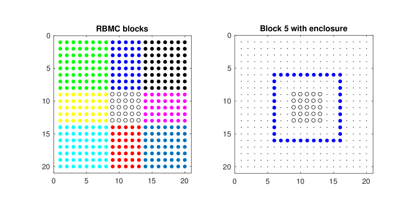
Figure 3.2. Disjoint blocks $\left\{\mathcal{Y}_{1},\ldots,\mathcal{Y}_{9}\right\}$ for block RBMC in different colors (left) and block 5 together with its spatial enclosure $\mathcal{I}\left(\mathcal{Y}_{5}\right)$ , that is, all nodes inside of the filled square (right).

3.1.1. Block RBMC

To compute the matrix diagonal using the improved RBMC estimator, we could use the following strategy. For each element $i$ we select a spatial enclosure $\mathcal{I}(i)$ of size $M$ and compute $\hat{\sigma}_{i|\mathcal{I}\left(i\right)^{c}}^{2}$ using Eq. (3.2). The computational bottleneck of the method will then be in the $N$ Cholesky factorizations of $M\times M$-matrices, needed to compute $\mathbf{Q}_{\mathcal{I}\left(i\right),\mathcal{I}\left(i\right)}^{-1}$ and $\boldsymbol{\kappa}_{\mathcal{I}\left(i\right)}^{\left(j\right)}$ for each $i$. In practice, this strategy might lead to substantial overhead costs when $N$ is large. In the numerical experiments in Section 4, we will therefore resort a to different strategy which we refer to as block RBMC. In block RBMC, we partition the domain into $N_{b}$ disjoint sets $\left\{\mathcal{Y}_{1},\ldots,\mathcal{Y}_{N_{b}}\right\}$ and compute $\hat{\boldsymbol{\Sigma}}_{\mathcal{Y}_{{}_{i}}|\mathcal{I}\left(\mathcal{Y}_{i}\right)^{c}}$ for each block $i$ using Eq. (3.2). An example for a 20 by 20 lattice and 9 blocks is displayed in Fig. 3.2.

When we are only interested in the covariance matrix diagonal, the important elements of Eq. (3.2) can be computed more efficiently. We start by reordering the nodes in the spatial enclosure $\mathcal{I}\left(\mathcal{Y}_{i}\right)$ using constrained approximate minimum degree (CAMD) reordering (Liu,, 1989; Amestoy et al.,, 1996), such that the block nodes $\mathcal{Y}_{i}$ comes last. Assuming $\left|\mathcal{I}\left(\mathcal{Y}_{i}\right)\right|$ is reasonably small, we can then compute the Cholesky factor of $\mathbf{Q}_{\mathcal{I}\left(\mathcal{Y}_{i}\right),\mathcal{I}\left(\mathcal{Y}_{i}\right)}$ cheaply and also the sparse inverse of $\mathbf{Q}_{\mathcal{I}\left(\mathcal{Y}_{i}\right),\mathcal{I}\left(\mathcal{Y}_{i}\right)}$ using the Takahashi equations (see Eq. (2.2)). Since we placed the block nodes last we do not need to iterate backwards the whole way to $i=1$ but can break as soon as the variances of the block nodes are computed. We thus have computed the first term of Eq. (3.2) and to obtain the second term we can compute $\boldsymbol{\kappa}_{\mathcal{I}\left(\mathcal{Y}_{i}\right)}^{\left(j\right)}$ for all $j$ with forward and backward substitution using the Cholesky factor. The block RBMC method is summarized in Algorithm 1. As presented there, block RBMC can be used to compute for example the covariance matrix diagonal. For some other possible choices of $\mathcal{S}$, trivial extensions to the algorithm could be required, including making the blocks overlapping and computing additional elements in the Takahashi equation step.

1:Precision matrix $\mathbf{Q}$, $N_{s}$ Gaussian samples $\mathbf{X}$,
blocks $\left\{\mathcal{Y}_{1},\ldots,\mathcal{Y}_{N_{b}}\right\}$, and block enclosures $\left\{\mathcal{I}\left(\mathcal{Y}_{1}\right),\ldots,\mathcal{I}\left(\mathcal{Y}_{N_{b}}\right)\right\}$

2:for  $i=1$ to $N_{b}$ do

3:     Reorder the nodes in $\mathcal{I}\left(\mathcal{Y}_{i}\right)$ using CAMD such that $\mathcal{Y}_{i}$ comes last

4:     Compute $\mathbf{L}_{\mathcal{I}\left(\mathcal{Y}_{i}\right)}$ as the Cholesky factor of $\mathbf{Q}_{\mathcal{I}\left(\mathcal{Y}_{i}\right),\mathcal{I}\left(\mathcal{Y}_{i}\right)}$

5:     for  $j=\left|\mathcal{I}\left(\mathcal{Y}_{i}\right)\right|$ to $\left|\mathcal{I}\left(\mathcal{Y}_{i}\right)\right|-\left|\mathcal{Y}_{i}\right|+1$ do

6:         Use the Takahashi equations to compute sparse elements $(j,k)$
.          of $\mathbf{Q}_{\mathcal{I}\left(\mathcal{Y}_{i}\right),\mathcal{I}\left(\mathcal{Y}_{i}\right)}^{-1}$, for $k\geq j$

7:     end for

8:     for  $j=1$ to $N_{s}$ do

9:         Solve $\mathbf{L}_{\mathcal{I}\left(\mathcal{Y}_{i}\right)}\tilde{\boldsymbol{\kappa}}=\mathbf{Q}_{\mathcal{I}\left(\mathcal{Y}_{i}\right),\mathcal{I}\left(\mathcal{Y}_{i}\right)^{c}}\mathbf{x}_{\mathcal{I}\left(\mathcal{Y}_{i}\right)^{c}}^{\left(j\right)}$  for $\tilde{\boldsymbol{\kappa}}$

10:         Solve $\mathbf{L}_{\mathcal{I}\left(\mathcal{Y}_{i}\right)}^{T}\boldsymbol{\kappa}_{\mathcal{I}\left(\mathcal{Y}_{i}\right)}^{\left(j\right)}=\tilde{\boldsymbol{\kappa}}$  for $\boldsymbol{\kappa}_{\mathcal{I}\left(\mathcal{Y}_{i}\right)}^{\left(j\right)}$

11:     end for

12:     Compute selected covariances in block $\mathcal{Y}_{i}$ using Eq. (3.2)

13:     Optionally compute the uncertainty measures using Eq. (3.3)

14:end for

Algorithm 1 Block RBMC

In the results presented in Section 4, the choices of blocks $\mathcal{Y}_{i}$ and enclosures $\mathcal{I}\left(\mathcal{Y}_{i}\right)$ will for simplicity be done correspondingly to how the blocks are chosen for the iterative interface method presented in Section 3.2 below. That is, for each block we select $\mathcal{Y}_{i}$ as the smallest rectangle (or cuboid in the 3D case) that contains all nodes in $\mathcal{Z}_{i}$ and $\mathcal{I}\left(\mathcal{Y}_{i}\right)=\mathcal{I}\left(\mathcal{W}_{i}\right)$ (see definitions of $\mathcal{Z}_{i}$ and $\mathcal{I}\left(\mathcal{W}_{i}\right)$ in Section 3.2, and the illustration in Fig. 3.3). This seems to be a pragmatic choice of blocks for the RBMC method in practice.

3.1.2. Approximation variance and confidence bounds

Precise estimates of the variance and uncertainty bounds of the different RBMC estimators can be cheaply obtained by noting that the estimator in Eq. (3.2) follows a Wishart distribution. See Mardia et al., (1979, Chapter 3) for some fundamental properties that connects the Wishart, Gaussian, and $\chi^{2}$-distributions. It can be seen that $\boldsymbol{\kappa}_{\mathcal{I}}^{\left(j\right)}$ in Eq. (3.2) is multivariate normal with mean zero and covariance matrix $\boldsymbol{\Sigma}_{\mathcal{I},\mathcal{I}}-\mathbf{Q}_{\mathcal{I},\mathcal{I}}^{-1}$ since $\mathbf{x}^{\left(j\right)}$ is normal and since the law of total variance gives that $\boldsymbol{\Sigma}_{\mathcal{I},\mathcal{I}}=\mathbf{Q}_{\mathcal{I},\mathcal{I}}^{-1}+Var\left(-\boldsymbol{\kappa}_{\mathcal{I}}^{\left(j\right)}\right)$. It thereby follows that

$$\hat{\boldsymbol{\Sigma}}_{\left(\mathcal{I},\mathcal{I}\right)|\mathcal{I}^{c}}\sim\mathbf{Q}_{\mathcal{I},\mathcal{I}}^{-1}+\frac{1}{N_{s}}\mathsf{Wishart}\left(\boldsymbol{\Sigma}_{\mathcal{I},\mathcal{I}}-\mathbf{Q}_{\mathcal{I},\mathcal{I}}^{-1},N_{s}\right),$$ (3.3)

and taking the mean directly shows the unbiasedness of the estimator.

We thus know the analytical distribution of the different RBMC estimators. This can be used to compute uncertainty measures such as the variances and confidence bounds of the different elements, apart from that we do not know $\boldsymbol{\Sigma}_{\mathcal{I},\mathcal{I}}$ which is in fact what we are trying to estimate. However, if $\hat{\boldsymbol{\Sigma}}_{\left(\mathcal{I},\mathcal{I}\right)|\mathcal{I}^{c}}$ is a reasonably good estimate of $\boldsymbol{\Sigma}_{\mathcal{I},\mathcal{I}}$, then plugging it into Eq. (3.3) instead of $\boldsymbol{\Sigma}_{\mathcal{I},\mathcal{I}}$ gives good estimates also of the uncertainty measures, as shown empirically in Section 4. Note that $\hat{\boldsymbol{\Sigma}}_{\left(\mathcal{I},\mathcal{I}\right)|\mathcal{I}^{c}}-\mathbf{Q}_{\mathcal{I},\mathcal{I}}^{-1}$ is positive definite, due to the construction in Eq (3.2). Also note that both $\hat{\boldsymbol{\Sigma}}_{\left(\mathcal{I},\mathcal{I}\right)|\mathcal{I}^{c}}$ and $\mathbf{Q}_{\mathcal{I},\mathcal{I}}^{-1}$ are already computed for selected elements in Algorithm 1, so computing the uncertainty measures generates very little additional computational cost.

As an example, we give explicit uncertainty measures for the RBMC estimates of the elements of covariance matrix diagonal $\hat{\sigma}_{i|\mathcal{I}^{c}}^{2}$. These can be derived by noting that the diagonal elements of a Wishart distributed matrix are $\chi^{2}$-distributed, so

$$\hat{\sigma}_{i|\mathcal{I}^{c}}^{2}\sim\left[\mathbf{Q}_{\mathcal{I},\mathcal{I}}^{-1}\right]_{i,i}+\frac{1}{N_{s}}\left(\sigma_{i}^{2}-\left[\mathbf{Q}_{\mathcal{I},\mathcal{I}}^{-1}\right]_{i,i}\right)\chi_{N_{s}}^{2},\,\,\,\,\,\,\,Var\left(\hat{\sigma}_{i|\mathcal{I}^{c}}^{2}\right)=\frac{2}{N_{s}}\left(\sigma_{i}^{2}-\left[\mathbf{Q}_{\mathcal{I},\mathcal{I}}^{-1}\right]_{i,i}\right)^{2},$$ (3.4)

and the quantiles of the $\chi^{2}$-distribution can directly be used to compute confidence intervals (CIs). In practice the uncertainty measures can be approximated using $\sigma_{i}^{2}=\hat{\sigma}_{i|\mathcal{I}^{c}}^{2}$.

3.2. Iterative interface method

In this section we introduce a method that can be used to further improve the RBMC covariance estimates by iterating over certain subdomains, which we call interfaces. For the ease of presentation, we will here assume that we have a GMRF defined on a 2D lattice with nearest neighbor Markov structure (5-point-stencil), but it is straightforward to extend this to 3D (we provide numerical results for this case in Section 4) and also possible for other types of domains or Markov structures. The underlying idea can be explained using Fig. 3.3, which depicts a $20$ by $20$ lattice with all the interface nodes marked with unfilled dots in the top left graph. The other three graphs illustrate situations in which a subset of interface nodes $\mathcal{W}_{i}$ (unfilled) have been enclosed within a frame of other interface nodes $\mathcal{V}_{i}$ (filled). The nodes in $\mathcal{W}_{i}$ are divided into an inner set $\mathcal{Z}_{i}$ (unfilled circles) and an outer set $\mathcal{W}_{i}\setminus\mathcal{Z}_{i}$ (unfilled squares) for reasons that will be apparent shortly. We also use the notation $\mathcal{I}\left(\mathcal{W}_{i}\right)$ for all nodes within the frame and $\mathcal{U}_{i}=\mathcal{I}\left(\mathcal{W}_{i}\right)\cup\mathcal{V}_{i}$, that is, $\mathcal{U}_{i}$ are all nodes on and inside the frame. Because of the Markov assumption, if we would know the covariance matrix $\boldsymbol{\Sigma}_{\mathcal{V}_{i},\mathcal{V}_{i}}$ of the frame, we could compute the covariance matrix of the inner nodes $\boldsymbol{\Sigma}_{\mathcal{W}_{i},\mathcal{W}_{i}}$ without having to consider the distribution outside of the frame. The basic idea is therefore to iterate between interface subdomains, as the three illustrated, and in each step compute the covariances of the inner nodes $\text{$\mathcal{W}$ }_{i}$ based on the covariances of the frame $\mathcal{V}_{i}$ and $\mathbf{Q}$ (for the example in Fig. 3.3, nine steps are required to iterate through all interface nodes once).

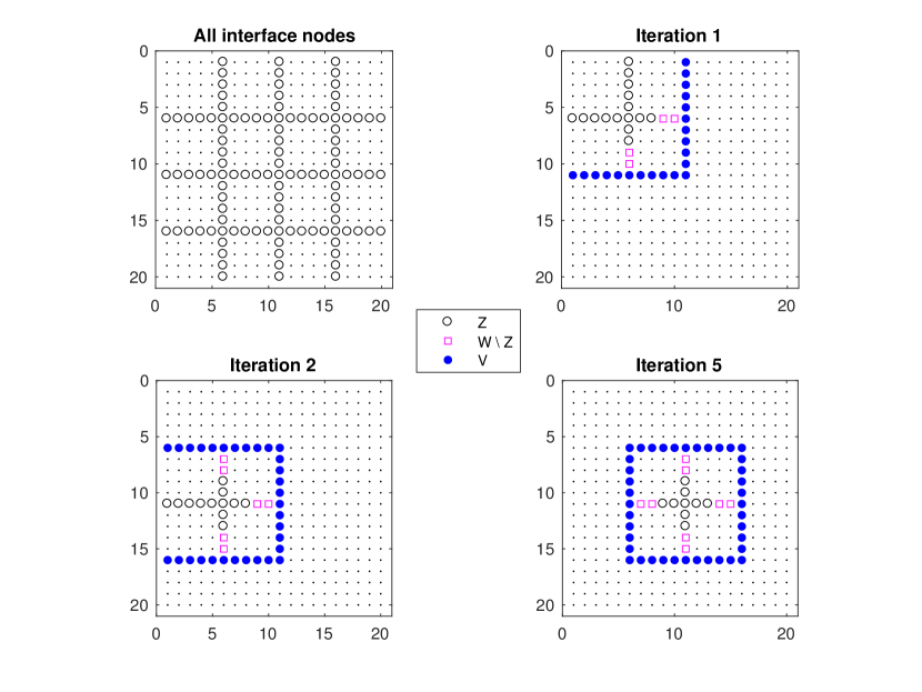
Figure 3.3. The iterative interface method illustrated for the $20$ by $20$ lattice with 9 subblocks. All interface nodes (top left) and those updated in the iterations 1, 2 and 5, divided into the sets $\mathcal{W}$, $\mathcal{V}$ and $\mathcal{Z}$. In addition, $\mathcal{I}\left(\mathcal{W}\right)$ denotes all nodes inside the frame and $\mathcal{U}$ denotes all nodes on and inside the frame $\mathcal{V}$.

The algorithm, summarized in Algorithm 2, can be divided into three phases. In the first phase, starting values are computed using a slightly modified version of the block RBMC method, in which the full covariance matrix of the innermost nodes $\mathcal{Z}_{i}$ are computed together with the cross-covariances between $\mathcal{Z}_{i}$ and $\mathcal{W}_{i}\setminus\mathcal{Z}_{i}$. The starting variances of the nodes in $\mathcal{W}_{i}\setminus\mathcal{Z}_{i}$ are however estimated in a different block where these nodes are further inside the frame, which leads to smaller error (consider for example the two bottommost square nodes in iteration 1 of Fig. 3.3, which are more centrally located in iteration 2). In the second phase the algorithm iterates $N_{iter}$ times over all $N_{b}$ blocks and computes $\boldsymbol{\Sigma}_{\mathcal{W}_{i},\mathcal{W}_{i}}$ each time treating $\boldsymbol{\Sigma}_{\mathcal{V}_{i},\mathcal{V}_{i}}$ as known. In the final phase all selected covariances (not only those that happen to belong to interface nodes) are computed using the Takahashi equations with the modification that the covariances on the frame, $\boldsymbol{\Sigma}_{\mathcal{V}_{i},\mathcal{V}_{i}}$, are treated as known. More formal derivations and motivations of the different steps in Algorithm 2 are given in the following subsection.

3.2.1. Algorithm derivation

Note that every step in Algorithm 2 is done within the context of a single subblock/interface, so here we drop the subindex $i$ from all sets, for readability. Consider the case when we are interested in computing the dense covariance matrix $\boldsymbol{\Sigma}_{\mathcal{W},\mathcal{W}}$ knowing $\boldsymbol{\Sigma}_{\mathcal{V},\mathcal{V}}$ and using that $p\left(\mathbf{x}_{\mathcal{W}}|\mathbf{x}_{\mathcal{V}}\,,\mathbf{x}_{\mathcal{U}^{c}}\right)=p\left(\mathbf{x}_{\mathcal{W}}|\mathbf{x}_{\mathcal{V}}\right).$ For computational efficiency, first reorder the nodes in $\mathbf{Q}_{\mathcal{I}\left(\mathcal{W}\right),\mathcal{I}\left(\mathcal{W}\right)}$ such that $\mathcal{W}$ comes last, using CAMD. Now, similar to when the RBMC method was derived

$$Var\left(\mathbf{x}_{\mathcal{I}\left(\mathcal{W}\right)}\right)=\boldsymbol{\Sigma}_{\mathcal{I}\left(\mathcal{W}\right),\mathcal{I}\left(\mathcal{W}\right)} =E\left[Var\left(\mathbf{x}_{\mathcal{I}\left(\mathcal{W}\right)}|\mathbf{x}_{\mathcal{V}}\right)\right]+Var\left[E\left(\mathbf{x}_{\mathcal{I}\left(\mathcal{W}\right)}|\mathbf{x}_{\mathcal{V}}\right)\right]$$

$$=\mathbf{Q}_{\mathcal{I}\left(\mathcal{W}\right),\mathcal{I}\left(\mathcal{W}\right)}^{-1}+Var\left(\mathbf{Q}_{\mathcal{I}\left(\mathcal{W}\right),\mathcal{I}\left(\mathcal{W}\right)}^{-1}\mathbf{Q}_{\mathcal{I}\left(\mathcal{W}\right),\mathcal{V}}\mathbf{x}_{\mathcal{V}}\right)$$

$$=\mathbf{L}^{-T}\mathbf{L}^{-1}+Var\left(\mathbf{L}^{-T}\mathbf{L}^{-1}\mathbf{Q}_{\mathcal{I}\left(\mathcal{W}\right),\mathcal{V}}\mathbf{x}_{\mathcal{V}}\right)$$

$$=\mathbf{L}^{-T}\left(\mathbf{I}_{\left|\mathcal{I}\left(\mathcal{W}\right)\right|}+Var\left(\mathbf{L}^{-1}\mathbf{Q}_{\mathcal{I}\left(\mathcal{W}\right),\mathcal{V}}\mathbf{x}_{\mathcal{V}}\right)\right)\mathbf{L}^{-1}$$

$$=\mathbf{L}^{-T}\left(\mathbf{I}_{\left|\mathcal{I}\left(\mathcal{W}\right)\right|}+\mathbf{M}\boldsymbol{\Sigma}_{V,V}\mathbf{M}^{T}\right)\mathbf{L}^{-1}$$ (3.5)

where $\mathbf{Q}_{\mathcal{I}\left(\mathcal{W}\right),\mathcal{I}\left(\mathcal{W}\right)}=\mathbf{LL}^{T}$ is the Cholesky decomposition and $\mathbf{M}=\mathbf{L}^{-1}\mathbf{Q}_{\mathcal{I}\left(\mathcal{W}\right),\mathcal{V}}$. This equation provides a way to compute $\boldsymbol{\Sigma}_{\mathcal{I}\left(\mathcal{W}\right),\mathcal{I}\left(\mathcal{W}\right)}$ when $\boldsymbol{\Sigma}_{\mathcal{V},\mathcal{V}}$ is known, but since we are only interested in the covariance matrix $\boldsymbol{\Sigma}_{\mathcal{W},\mathcal{W}}$, this would be unnecessary. We divide the Cholesky factor $\mathbf{L}$ using the subsets $\mathcal{\widetilde{\mathcal{W}}}:=\mathcal{I}\left(\mathcal{W}\right)\setminus\mathcal{W}$ and $\mathcal{W}$ so that

$$\mathbf{L}=\left[\begin{array}[]{cc}\mathbf{L}_{\mathcal{\widetilde{\mathcal{W}}}}\\ \mathbf{L}_{\mathcal{W},\mathcal{\widetilde{\mathcal{W}}}}&\mathbf{L}_{\mathcal{W}}\end{array}\right]\Rightarrow\mathbf{L}^{-1}=\left[\begin{array}[]{cc}\mathbf{L}_{\mathcal{\widetilde{\mathcal{W}}}}^{-1}\\ -\mathbf{L}_{\mathcal{W}}^{-1}\mathbf{L}_{\mathcal{W},\mathcal{\widetilde{\mathcal{W}}}}\mathbf{L}_{\mathcal{\widetilde{\mathcal{W}}}}^{-1}&\mathbf{L}_{\mathcal{W}}^{-1}\end{array}\right]=\left[\begin{array}[]{cc}\mathbf{L}_{\mathcal{\widetilde{\mathcal{W}}}}^{-1}\\ -\mathbf{S}&\mathbf{L}_{\mathcal{W}}^{-1}\end{array}\right],$$ (3.6)

and divide $\mathbf{M}$ as $\ \mathbf{M}^{T}=\left[\text{{M}}_{\mathcal{\widetilde{\mathcal{W}}}}^{T}\,\,\mathbf{M}_{\mathcal{W}}^{T}\right]$. Eq. (3.5) can now be written as

$$\left[\begin{array}[]{cc}\boldsymbol{\Sigma}_{\mathcal{\widetilde{\mathcal{W}}},\mathcal{\widetilde{\mathcal{W}}}}&\boldsymbol{\Sigma}_{\mathcal{\widetilde{\mathcal{W}}},\mathcal{W}}\\ \boldsymbol{\Sigma}_{\mathcal{W},\mathcal{\widetilde{\mathcal{W}}}}&\boldsymbol{\Sigma}_{\mathcal{W},\mathcal{W}}\end{array}\right] =\left[\begin{array}[]{cc}\mathbf{L}_{\mathcal{\widetilde{\mathcal{W}}}}^{-T}&-\mathbf{S}\\ &\mathbf{L}_{\mathcal{W}}^{-T}\end{array}\right]\cdot$$ (3.11)

$$\left(\left[\begin{array}[]{cc}\mathbf{I}_{\left|\mathcal{\widetilde{\mathcal{W}}}\right|}+\mathbf{M}_{\mathcal{\widetilde{\mathcal{W}}}}\boldsymbol{\Sigma}_{\mathcal{V},\mathcal{V}}\mathbf{M}_{\mathcal{\widetilde{\mathcal{W}}}}^{T}&\mathbf{M}_{\mathcal{\widetilde{\mathcal{W}}}}\boldsymbol{\Sigma}_{\mathcal{V},\mathcal{V}}\mathbf{M}_{\mathcal{W}}^{T}\\ \mathbf{M}_{\mathcal{W}}\boldsymbol{\Sigma}_{\mathcal{V},\mathcal{V}}\mathbf{M}_{\mathcal{\widetilde{\mathcal{W}}}}^{T}&\mathbf{I}_{\left|\mathcal{W}\right|}+\mathbf{M}_{\mathcal{W}}\boldsymbol{\Sigma}_{\mathcal{V},\mathcal{V}}\mathbf{M}_{\mathcal{W}}^{T}\end{array}\right]\right)\left[\begin{array}[]{cc}\mathbf{L}_{\mathcal{\widetilde{\mathcal{W}}}}^{-1}\\ -\mathbf{S}&\mathbf{L}_{\mathcal{W}}^{-1}\end{array}\right],$$ (3.16)

from which the bottom right block can be extracted. This gives

$$\boldsymbol{\Sigma}_{\mathcal{W},\mathcal{W}}=\mathbf{L}_{\mathcal{W}}^{-T}\left(\mathbf{I}_{\left|\mathcal{W}\right|}+\mathbf{M}_{\mathcal{W}}\boldsymbol{\Sigma}_{\mathcal{V},\mathcal{V}}\mathbf{M}_{\mathcal{W}}^{T}\right)\mathbf{L}_{\mathcal{W}}^{-1},$$ (3.17)

and we now have a formula to update $\boldsymbol{\Sigma}_{W,W}$ given $\boldsymbol{\Sigma}_{\mathcal{V},\mathcal{V}}$, which is used on line 10 in Algorithm 2. If $\boldsymbol{\Sigma}_{\mathcal{V},\mathcal{V}}$ is approximated by samples in Eq. (3.17) we get the RBMC estimator for the starting values in line 5

$$\boldsymbol{\hat{\Sigma}}_{\mathcal{W},\mathcal{W}}^{\text{start}}=\mathbf{L}_{\mathcal{W}}^{-T}\left(\mathbf{I}_{\left|\mathcal{W}\right|}+\frac{1}{N_{s}}\sum_{j=1}^{N_{s}}\left(\mathbf{M}_{\mathcal{W}}\mathbf{x}_{\mathcal{V}}^{\left(j\right)}\right)\left(\mathbf{M}_{\mathcal{W}}\mathbf{x}_{\mathcal{V}}^{\left(j\right)}\right)^{T}\right)\mathbf{L}_{\mathcal{W}}^{-1}.$$ (3.18)

1:Precision matrix $\mathbf{Q}$, Gaussian samples $\mathbf{X}$,
and node sets $\mathcal{W}_{i}$, $\mathcal{I}\left(\mathcal{W}_{i}\right)$, $\mathcal{V}_{i}$, $\mathcal{Z}_{i}$, $\mathcal{U}_{i}$ for all $i$

2:for  $i=1$ to $N_{b}$ do $\triangleright$ start phase one

3:     Reorder the nodes in $\mathcal{I}\left(\mathcal{W}_{i}\right)$ using CAMD such that $\mathcal{W}_{i}$ comes last

4:     Compute $\mathbf{L}$ as the Cholesky factor of $\mathbf{Q}_{\mathcal{I}\left(\mathcal{W}_{i}\right),\mathcal{I}\left(\mathcal{W}_{i}\right)}$ and extract $\mathbf{L}_{\mathcal{W}_{i}}$ as
.     the bottom right $\left|\mathcal{W}_{i}\right|\times\left|\mathcal{W}_{i}\right|$ block of $\mathbf{L}$

5:     Compute $\mathbf{M}=\mathbf{L}^{-1}\mathbf{Q}_{\mathcal{I}\left(\mathcal{W}_{i}\right),\mathcal{V}_{i}}$ and extract $\mathbf{M}_{\mathcal{W}_{i}}$ as the last $\left|\mathcal{W}_{i}\right|$ rows of $\mathbf{M}$

6:     Compute starting values as
.     $\boldsymbol{\hat{\Sigma}}_{\mathcal{W}_{i},\mathcal{W}_{i}}^{\text{start}}=\mathbf{L}_{\mathcal{W}_{i}}^{-T}\left(\mathbf{I}_{\left|\mathcal{W}_{i}\right|}+\frac{1}{N_{s}}\sum_{j=1}^{N_{s}}\left(\mathbf{M}_{\mathcal{W}_{i}}\mathbf{x}_{\mathcal{V}_{i}}^{\left(j\right)}\right)\left(\mathbf{M}_{\mathcal{W}_{i}}\mathbf{x}_{\mathcal{V}_{i}}^{\left(j\right)}\right)^{T}\right)\mathbf{L}_{\mathcal{W}_{i}}^{-1}$

7:     Set $\boldsymbol{\hat{\Sigma}}_{\mathcal{S}}=\boldsymbol{\hat{\Sigma}}_{\mathcal{S}}^{\text{start}}$ for $\mathcal{S}=\left(\mathcal{Z}_{i}\times\mathcal{Z}_{i}\right)\cup\left(\left(\mathcal{W}_{i}\setminus\mathcal{Z}_{i}\right)\times\mathcal{Z}_{i}\right)\cup\left(\mathcal{Z}_{i}\times\left(\mathcal{W}_{i}\setminus\mathcal{Z}_{i}\right)\right)$

8:end for

9:for  $j=1$ to $N_{iter}$ do $\triangleright$ start phase two

10:     for  $i=1$ to $N_{b}$ do

11:         Compute $\boldsymbol{\hat{\Sigma}}_{\mathcal{W}_{i},\mathcal{W}_{i}}=\mathbf{L}_{\mathcal{W}_{i}}^{-T}\left(\mathbf{I}_{\left|\mathcal{W}_{i}\right|}+\mathbf{M}_{\mathcal{W}_{i}}\boldsymbol{\hat{\Sigma}}_{\mathcal{V}_{i},\mathcal{V}_{i}}\mathbf{M}_{\mathcal{W}_{i}}^{T}\right)\mathbf{L}_{\mathcal{W}_{i}}^{-1}$

12:     end for

13:end for

14:for  $i=1$ to $N_{b}$ do $\triangleright$ start phase three

15:     Reorder the nodes in $\mathcal{U}_{i}$ using CAMD such that $\mathcal{V}_{i}$ comes last

16:     Compute $\mathbf{L}_{\mathcal{U}_{i}}$ as the Cholesky factor of $\mathbf{Q}_{\mathcal{U}_{i},\mathcal{U}_{i}}$

17:     for  $j=\left|\mathcal{I}\left(\mathcal{W}_{i}\right)\right|$ to $1$ do

18:         Use the Takahashi equations to compute sparse elements $(j,k)$
.          of $\boldsymbol{\hat{\Sigma}}_{\mathcal{U}_{i},\mathcal{U}_{i}}$, for $k\geq j$ treating the last block $\boldsymbol{\hat{\Sigma}}_{\mathcal{V}_{i},\mathcal{V}_{i}}$ as known.

19:     end for

20:end for

Algorithm 2 Iterative interface method

3.2.2. Convergence and error

The hope is to bring the interface covariances closer to the exact values in each iteration. However, the error will not converge to zero in general since the necessary covariances between some nodes in each frame can not be computed, and will instead be assumed to be zero. For example, in the bottom right subgraph of Fig 3.3, the covariance between the top left and bottom right nodes in the frame will never be computed since these nodes are not in the same $\mathcal{W}_{i}$ for any $i$. Still, for all interface nodes that are close to each other the covariance will be computed in some block $i$ and hopefully the approximation error from not computing the covariance of distant nodes will be small. If not we can always increase the sizes of the interface blocks, which increases the distance between the nodes for which the covariance can not be computed. This will however bring additional computational costs.

3.3. Correcting for linear constraints

A situation that occurs quite frequently in practice is that we have some linear constraints $\mathbf{Ax}=\mathbf{e}$ on the GMRF $\mathbf{x}$, for example that $\sum_{i}x_{i}=0$, that is $\mathbf{A}=\mathbf{1}^{T}$ and $\mathbf{e}=0$ (Rue and Held,, 2005). In such a situation, Rue and Martino, (2007) provide a general strategy to compute selected elements of the covariance matrix $\boldsymbol{\Sigma}^{*}$ of $\mathbf{x}^{*}=\left(\mathbf{x}|\mathbf{Ax}=\mathbf{e}\right)$ using that

$$\boldsymbol{\Sigma}^{*}=\boldsymbol{\Sigma}-\mathbf{Q}^{-1}\mathbf{A}^{T}\left(\mathbf{A}\mathbf{Q}^{-1}\mathbf{A}^{T}\right)^{-1}\mathbf{A}\mathbf{Q}^{-1}=\boldsymbol{\Sigma}-\mathbf{W}\left(\mathbf{A}\mathbf{W}\right)^{-1}\mathbf{W}^{T}=\boldsymbol{\Sigma}-\mathbf{C},$$ (3.19)

where $\mathbf{W}=\mathbf{Q}^{-1}\mathbf{A}^{T}$ and $\mathbf{C}=\mathbf{W}\left(\mathbf{A}\mathbf{W}\right)^{-1}\mathbf{W}^{T}$. If $\mathbf{A}$ is of size $k\times N$, then the cost of computing $\mathbf{W}$ is equal to that of solving $k$ equation systems $\mathbf{Q}\mathbf{W}=\mathbf{A}^{T}$, which can be done with PCG as explained earlier, as long as $k$ is reasonably small. In this case, computing selected elements of $\mathbf{C}$ is also cheap, requiring one $k\times k$ matrix inversion and an additional $k\times k$ matrix-vector-multiplication per element. Thereby, given an estimate $\hat{\boldsymbol{\Sigma}}_{\mathcal{S}}$ for some index set $\mathcal{S}$ from any of the methods above, an estimate $\hat{\boldsymbol{\Sigma}}_{\mathcal{S}}^{*}=\hat{\boldsymbol{\Sigma}}_{\mathcal{S}}-\mathbf{C}_{\mathcal{S}}$ of selected elements of the covariance matrix of the constrained field is straightforward to compute. As $\mathbf{C}_{\mathcal{S}}$ can be computed exactly the variance of the estimator $\hat{\boldsymbol{\Sigma}}_{\mathcal{S}}^{*}$ is the same as the variance of $\hat{\boldsymbol{\Sigma}}_{\mathcal{S}}$.

When this method is used for the diagonal elements of $\boldsymbol{\Sigma}^{*}$, the marginal variances, some attention should be drawn to the fact that some estimates could become negative if $\hat{\boldsymbol{\Sigma}}_{i,i}<\mathbf{C}_{i,i}$ for some $i$. One possible approach to remedy this situation in practice is to replace any negative estimates with the MC estimates computed using samples from the constrained field itself (with subtracted mean), which can be computed by correcting the samples from the original field as $\mathbf{X}^{*}=\mathbf{X}-\mathbf{W}\left(\mathbf{A}\mathbf{W}\right)^{-1}\mathbf{A}\mathbf{X},$ see Rue and Held, (2005, Algortihm 2.6).

4. Results

In this section, we will investigate the performance of the introduced methods for selected inversion empirically on various posterior precision matrices. We first compare sampling-based methods on a simple theoretical model and then consider a spatial model for neuroimaging and evaluate all our methods using data from both simulated and real fMRI experiments. All computations were performed on a Linux workstation with a 4-core (8 threads) Intel Xeon E5-1620 processor at 3.5GHz and 128GB RAM. The main part of the code was written in Matlab, but some (non-optimized) C++ code was called for evaluating the Takahashi equations and the SuiteSparse library (Davis,, 2017) was used for calling CAMD and the functions for symbolic Cholesky factorization.

The first task consists in computing the covariance matrix diagonal corresponding to the sparse posterior matrix of a simple model with independent Gaussian measurements and a first order random walk prior on the 3D lattice, that is $y_{i}\sim\mathsf{N}\left(x_{i},\lambda_{i}^{-1}\right)$ and $x_{i}-x_{j}\sim\mathsf{N}\left(0,1\right)$ for all adjacent nodes $i$ and $j$ on the lattice a priori. $\lambda_{i}$ were uniformly sampled on the interval $\left(0.1,0.2\right)$ for all $i$. The posterior distribution for $\mathbf{x}|\mathbf{y}$ is a GMRF with precision matrix $\mathbf{Q}=diag\left(\boldsymbol{\lambda}\right)+\mathbf{G}^{T}\mathbf{G}$, with $\boldsymbol{\lambda}=\left[\lambda_{1},\ldots,\lambda_{N}\right]$ and $\mathbf{G}$ is a matrix with one row for every pair of adjacent nodes $i$ and $j$, with $1$ in column $i$ and $-1$ in column $j$. We compare the simple RBMC and block RBMC methods to the MC and Hutchinson sampling-based methods in Table 1. For each node $i$ we compute the relative error $r_{i}=\nicefrac{{\left(\hat{\sigma}_{i}^{2}-\sigma_{i}^{2}\right)}}{{\sigma_{i}^{2}}}$ using $\sigma_{i}^{2}$ computed exactly using the Takahashi equations. The maximum error is computed as $\max_{i}\left|r_{i}\right|$ and the RMSE is computed empirically for $r_{i}$ across all nodes for each method. For each $\hat{\sigma}_{i}^{2}$ for the block RBMC method, we also compute a confidence interval (CI) based on the $\chi^{2}$-distribution in Eq. (3.4), with $\sigma_{i}^{2}=\hat{\sigma}_{i|\mathcal{I}^{c}}^{2}$, and count the share of nodes for which the true value $\sigma_{i}^{2}$ is outside the CI. The CI computation for the MC method uses that $\hat{\sigma}_{MC,i}^{2}\sim\frac{\sigma_{i}^{2}}{N_{s}}\chi_{N_{s}}^{2}$. For the Hutchinson method we do not have a simple method to compute CIs, so this measure is not reported. The lattice is of size $80\times 80\times 80=512,000$ and for block RBMC we use 5, 10 or 20 blocks in each dimension and we present results using 20 and 100 random samples.

Table 1. Computing times, empirical errors and proportion of confidence intervals not covering the true value when computing the posterior covariance matrix diagonal of a theoretical spatial model on a $80\times 80\times 80$ lattice, using different methods and different number of random samples. The presented results are averages $\pm$ one standard deviation across 100 runs with different random seeds.

Table 1 clearly shows that our simple RBMC method performs significantly better than previous methods (MC and Hutchinson) with the same computing time. We see that the error can be further decreased using the block RBMC method, but with additional computational cost. If low error is desirable, the results indicate that block RBMC with few samples is preferable over simple RBMC with many samples, as block RBMC with 1000 blocks and 20 samples gives far lower error than simple RBMC with 100 samples, in less time. Out of the two previous methods, Hutchinson seems to give lower error than MC, but we noted a drawback in that Hutchinson can sometimes produce negative variance estimates. The computed CIs can be seen to cover close to the desired $95\%$ of the true values, but they are slightly biased because $\hat{\sigma}_{i}^{2}$ is used in place of $\sigma_{i}^{2}$. The bias is reduced when using a larger number of samples, and since it is so systematic it could probably be corrected for, knowing the distribution of $\hat{\sigma}_{i}^{2}$. However, for most applications, this level of error in the uncertainty of the estimated covariances is likely to be acceptable, so we leave such a task to future work.

Next, we consider a spatial regression model for neuroimaging (Sidén et al.,, 2017; Penny et al.,, 2007). Brain activity is modeled as a GMRF on a 3D lattice of voxels over the brain, with $K$ different variables in each voxel, corresponding to activations of different tasks and an intercept. The resulting variational Bayes (VB) posterior is a GMRF of size $KN$, where $N$ is the number of voxels, and the Markov assumptions of the model makes all non-adjacent voxels conditionally independent. This makes the use of our developed methods possible, if we for the iterative interface include all $K$ variables in each voxel on for example the frame to the corresponding interface set $\mathcal{V}_{i}$. We present results for the block RBMC and iterative interface methods in Table 2 for data simulated in the same way as in Sidén et al., (2017, Appendix D) on a $50\times 50\times 40$ lattice and $K=5$ (the resulting GMRF has $500,000$ variables). The errors are computed relative to the exact values computed using the Takahashi equations. We use $N_{s}=20$ samples in $\mathbf{X}$ for both methods and our experience has shown that the iterative interface methods does not improve much after the first iteration, so we use $N_{iter}=1$, and we use 5, 10 and 15 interface blocks in each of the three dimensions.

Table 2 shows that the iterative interface method can reduce the error beyond what is achievable using the block RBMC method, but that it requires more computing time and memory. The computing time of the exact Takahashi equations could probably be significantly reduced by optimizing the code, but its large memory requirements (55GB) is just that of storing the Cholesky factor and the corresponding sparse inverse of $\mathbf{Q}$, which is difficult to reduce further, showing the infeasibility of exact methods for large problems. The iterative interface method can also be rather costly memory-wise, but by choosing the appropriate block sizes one could adapt the memory usage to the current limitations.

Table 2. Computing times, memory usage and errors relative to the exact values from the Takahashi equations, when computing the posterior covariance matrix of the spatial model in Sidén et al., (2017) using simulated fMRI data on a $50\times 50\times 40$ with a 5-dimensional variable in each lattice point, using different methods and different number of blocks and $20$ random samples. The presented results are averages $\pm$ one standard deviation across 10 runs with different random seeds, except for the Takahashi equations.

So far we have only evaluated the methods on marginal variances, but the methods can be used to estimate all covariances. To show that the error is small also for the covariances we computed the empirical absolute RMSE for $\hat{\Sigma}_{i,j}$ across all $i$ and $j$ corresponding to the same variable in adjacent voxels, estimated with the iterative interface method with 1000 blocks (the relative RMSE is not suitable for covariances as they can be zero or negative). The RMSE was $4.04\cdot 10^{-5}$ for these off-diagonal elements, which can be compared to $3.02\cdot 10^{-5}$ for the diagonal elements, indicating that the errors are in the same order of magnitude.

Finally, we visualize the improvement of our methods on some real fMRI data. The top left subfigure in Fig. 4.1 replicates the bottom middle subfigure in Sidén et al., (2017, Fig. 3), showing MC estimated marginal standard deviations of brain activity over a brain slice. The top right subfigure shows the ratio ($\hat{\sigma}_{i}/\sigma_{i}$) compared to the exact marginal standard deviations computed with the Takahashi equations. The bottom row shows the same, but with simple RBMC estimates instead of MC. It is clear that the simple RBMC estimates have much smaller error and using the even more exact block RBMC or iterative interface methods would reduce the error to levels that would be hardly visible to the naked eye.

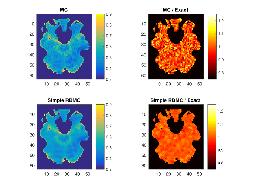
Figure 4.1. Posterior marginal standard deviation estimates for the fMRI data and model in Sidén et al., (2017), based on MC estimation (top row) and simple RBMC estimation (bottom row). The second column shows the estimated standard deviations divided with the exact values, computed using the slower Takahashi equations method.

5. Discussion and future work

The results show that our suggested methods, the simple RBMC, the block RBMC, and the iterative interface method outperform other sampling-based methods in terms of accuracy for a given computing time, and exact methods in terms of memory usage.

For a practical problem, one could find the desired balance between error, computing time and memory requirements by choosing between our proposed methods, the number of samples and the number of blocks (or block sizes). For the RBMC methods, the error will decrease linearly with $\sqrt{N_{s}}$, while time and memory requirements grow linearly with $N_{s}$. As usual with Monte Carlo methods this gives asymptotical exactness, but this limit is not attainable in practice.

Both the RBMC and iterative interface methods also converges with block size, as $N_{b}=1$ will be the same as the exact Takahashi equations. Exactly how the error, computing time and memory depend on the block sizes is a difficult question to answer in general, but by assuming a field that is fairly stationary, the following strategy could be employed to find the required block size for a given error: Compute the block RBMC estimates for just one or a small number of blocks and also compute the corresponding uncertainty measures, as explained in Section 3.1.2. Redo this procedure with increasing block sizes until the uncertainty is sufficiently small, before computing the estimates for the whole domain. Since the iterative interface method uses block RBMC for starting values and then reduces the error, this gives an upper bound for the uncertainty also for that method. Especially, models with longer spatial correlation range will require larger blocks to obtain a given accuracy.

There are a number of ways in which our algorithms can be parallelized. All samples in $\mathbf{X}$ are independent, so these can be generated in parallel. Also, all steps in the RBMC and iterative interface methods are done independently for each block and are straightforward to parallelize over blocks, apart from phase two in the iterative interface method, but this phase can probably be run in parallel by letting different threads operate on separate parts of the domain.

As we mentioned in Section 2, our developed methods can be used for trace estimation needed for EM and VB, but they could also be used in other methods, for example integrated nested Laplace approximation (INLA) (Rue et al.,, 2009). INLA normally uses the Cholesky factor of $\mathbf{Q}$ for computing marginal posterior variances and $\log\text{$\left|\textbf{Q}\right|$}$. To avoid the Cholesky factorization, the variances could instead be approximated using our methods and the log determinant could be approximated for example using the methods in Aune et al., (2014) or Ubaru et al., (2017). The usefulness of our methods within MCMC algorithms is probably limited, as posterior samples can normally be sampled using $\mathbf{Q}$ directly with for example the method in Papandreou and Yuille, (2010), without the need of computing elements of the covariance matrix. However, our algorithms could possibly be employed in MCMC post processing to more efficiently compute marginal variances. The usefulness of our methods for models not always formulated using precision matrices such as vector autoregressive (VAR) models (Koop,, 2013) and could also be further explored.

6. Conclusions

We presented a number of methods for estimating selected elements of the covariance matrix when the precision matrix is sparse and the corresponding Gaussian density can be sampled from, but too large for full inversion or even Cholesky factorization. Our methods extends the idea of Papandreou and Yuille, (2010) to use MC sampling to estimate covariances, but better utilizes the information from the known precision matrix to reduce the error, while simultaneously having lower computational requirements than known exact methods.

References

- Amestoy et al., (1996) Amestoy, P. R., Davis, T. A., and Duff, I. S. (1996). An approximate minimum degree ordering algorithm. SIAM Journal on Matrix Analysis and Applications, 17(4):886–905.
- Amestoy et al., (2012) Amestoy, P. R., Duff, I. S., L’Excellent, J.-Y., Robert, Y., Rouet, F.-H., and Uçar, B. (2012). On computing inverse entries of a sparse matrix in an out-of-core environment. SIAM Journal on Scientific Computing, 34(4):A1975–A1999.
- Amestoy et al., (2015) Amestoy, P. R., Duff, I. S., L’Excellent, J.-Y., and Rouet, F.-H. (2015). Parallel computation of entries of A^-1. SIAM Journal on Scientific Computing, 37(2):C268–C284.
- Aune et al., (2014) Aune, E., Simpson, D. P., and Eidsvik, J. (2014). Parameter estimation in high dimensional Gaussian distributions. Statistics and Computing, 24(2):247–263.
- Barrett et al., (1994) Barrett, R., Berry, M. W., Chan, T. F., Demmel, J., Donato, J., Dongarra, J., Eijkhout, V., Pozo, R., Romine, C., and Van der Vorst, H. (1994). Templates for the solution of linear systems: building blocks for iterative methods, volume 43. Siam, Philadelphia, PA.
- Beaky et al., (1992) Beaky, M. M., Scherrer, R. J., and Villumsen, J. V. (1992). Topology of large-scale structure in seeded hot dark matter models. The Astrophysical Journal, 387:443–448.
- Bekas et al., (2007) Bekas, C., Kokiopoulou, E., and Saad, Y. (2007). An estimator for the diagonal of a matrix. Applied Numerical Mathematics, 57:1214–1229.
- Besag, (1974) Besag, J. (1974). Spatial interaction and the statistical analysis of lattice systems. Journal of the Royal Statistical Society. Series B (Methodological), 36(2):192–236.
- Bhattacharya et al., (2016) Bhattacharya, A., Chakraborty, A., and Mallick, B. K. (2016). Fast sampling with Gaussian scale-mixture priors in high-dimensional regression. Biometrika, 103(4):985–991.
- Bolin and Lindgren, (2015) Bolin, D. and Lindgren, F. (2015). Excursion and contour uncertainty regions for latent Gaussian models. Journal of the Royal Statistical Society: Series B (Statistical Methodology), 77(1):85–106.
- Bolin et al., (2009) Bolin, D., Lindström, J., Eklundh, L., and Lindgren, F. (2009). Fast estimation of spatially dependent temporal vegetation trends using Gaussian Markov random fields. Computational Statistics and Data Analysis, 53(8):2885–2896.
- Davis, (2017) Davis, T. A. (2017). SuiteSparse. http://faculty.cse.tamu.edu/davis/research.html.
- Erisman and Tinney, (1975) Erisman, a. M. and Tinney, W. F. (1975). On computing certain elements of the inverse of a sparse matrix. Communications of the ACM, 18(3):177–179.
- Furrer et al., (2007) Furrer, R., Knutti, R., Sain, S. R., Nychka, D. W., and Meehl, G. A. (2007). Spatial patterns of probabilistic temperature change projections from a multivariate Bayesian analysis. Geophysical Research Letters, 34(6):2–5.
- Hutchinson, (1990) Hutchinson, M. F. (1990). A stochastic estimator of the trace of the influence matrix for Laplacian smoothing splines. Communications in Statistics-Simulation and Computation, 19(2):433–450.
- Jacquelin et al., (2015) Jacquelin, M., Lin, L., and Yang, C. (2015). PSelInv - A distributed memory parallel algorithm for selected inversion : the symmetric case. arXiv preprint 1404.0447v3.
- Jeng and Woods, (1991) Jeng, F. C. and Woods, J. W. (1991). Compound Gauss-Markov random fields for image estimation. IEEE Transactions on Signal Processing, 39(3):683–697.
- Koop, (2013) Koop, G. M. (2013). Forecasting with medium and large Bayesian VARs. Journal of Applied Econometrics, 28(2):117–203.
- Lauritzen, (1996) Lauritzen, S. L. (1996). Graphical models, volume 17. Clarendon Press.
- Li et al., (2008) Li, S., Ahmed, S., Klimeck, G., and Darve, E. (2008). Computing entries of the inverse of a sparse matrix using the FIND algorithm. Journal of Computational Physics, 227(22):9408–9427.
- (21) Lin, L., Yang, C., Lu, J., Ying, L., and Weinan, E. (2011a). A fast parallel algorithm for selected inversion of structured sparse matrices with application to 2D electronic structure calculations. SIAM Journal on Scientific Computing, 33(3):1329–1351.
- (22) Lin, L., Yang, C., Meza, J. C., Lu, J., Ying, L., and E, W. (2011b). SelInv–An algorithm for selected inversion of a sparse symmetric matrix. ACM Transactions on Mathematical Software, 37(4):1–19.
- Liu, (1989) Liu, J. W. H. (1989). The minimum degree ordering with constraints. SIAM Journal on Scientific and Statistical Computing, 10(6):1136–1145.
- Liu et al., (2012) Liu, Y., Chandrasekaran, V., Anandkumar, A., and Willsky, A. S. (2012). Feedback message passing for inference in Gaussian graphical models. IEEE Transactions on Signal Processing, 60(8):4135–4150.
- Malioutov et al., (2008) Malioutov, D. M., Johnson, J. K., Choi, M. J., and Willsky, A. S. (2008). Low-rank variance approximation in GMRF models: Single and multiscale approaches. IEEE Transactions on Signal Processing, 56(10):4621–4634.
- Malioutov et al., (2006) Malioutov, D. M., Johnson, J. K., and Willsky, A. S. (2006). Walk-sums and belief propagation in Gaussian graphical models. Journal of Machine Learning Research, 7:2031–2064.
- Manteuffel, (1980) Manteuffel, T. a. (1980). An incomplete factorization technique for positive definite linear systems. Mathematics of Computation, 34(150):473–473.
- Mardia et al., (1979) Mardia, K. V., Kent, J. T., and Bibby, J. M. (1979). Multivariate analysis. Academic Press.