Which bridge estimator is The Best For Variable Selection?

Abstract

We study the problem of variable selection for linear models under the high-dimensional asymptotic setting, where the number of observations $n$ grows at the same rate as the number of predictors $p$. We consider two-stage variable selection techniques (TVS) in which the first stage uses bridge estimators to obtain an estimate of the regression coefficients, and the second stage simply thresholds this estimate to select the “important” predictors. The asymptotic false discovery proportion (AFDP) and true positive proportion (ATPP) of these TVS are evaluated. We prove that for a fixed ATPP, in order to obtain a smaller AFDP, one should pick a bridge estimator with smaller asymptotic mean square error in the first stage of TVS. Based on such principled discovery, we present a sharp comparison of different TVS, via an in-depth investigation of the estimation properties of bridge estimators. Rather than “order-wise” error bounds with loose constants, our analysis focuses on precise error characterization. Various interesting signal-to-noise ratio and sparsity settings are studied. Our results offer new and thorough insights into high-dimensional variable selection. For instance, we prove that a TVS with Ridge in its first stage outperforms TVS with other bridge estimators in large noise settings; two-stage LASSO becomes inferior when the signal is rare and weak. As a by-product, we show that two-stage methods outperform some standard variable selection techniques, such as LASSO and Sure Independence Screening, under certain conditions.

and

1 Introduction

1.1 Motivation and problem statement

Although linear models can be traced back to two hundred years ago, they keep shining in the modern statistical research. A problem of major interest in this literature is variable selection. Consider the linear regression model

$$y=X\beta+w,$$

with $y\in\mathbb{R}^{n}$, $X\in\mathbb{R}^{n\times p}$, $\beta\in\mathbb{R}^{p}$ and $w\in\mathbb{R}^{n}$. Suppose only a few elements of $\beta$ are nonzero. The problem of variable selection is to find these nonzero locations of $\beta$. Motivated by the concerns about the instability and high computational cost of classical variable selection techniques, such as best subset selection and stepwise selection, Tibshirani proposed LASSO [Tib96] to perform parameter estimation and variable selection simultaneously. The LASSO estimate is given by

$$\hat{\beta}(1,\lambda):=\underset{\beta}{\text{argmin}}\;\frac{1}{2}\|y-X\beta\|_{2}^{2}+\lambda\|\beta\|_{1},$$ (1.1)

where $\lambda\in(0,\infty)$ is the tuning parameter, and $\|\cdot\|_{1}$ is the $\ell_{1}$ norm. The regularization term $\|\beta\|_{1}$ stablizes the variable selection process while the convex formulation of (1.1) reduces the computational cost.

Compared to LASSO, other convex regularizers such as $\|\beta\|_{2}^{2}$ imposes larger penalty to large components of $\beta$. Hence, their estimates might be more stable than LASSO. Even though the solutions of many of these regularizers are not sparse (and thus not automatically perform variable selection), we may threshold their estimates to select variables. This observation leads us to the following questions: can such two-stage methods with other regularizers outperform LASSO in variable selection? If so, which regularizer should be used in the first stage? The goal of this paper is to address these questions. In particular, we study the performances of the two-stage variable selection (TVS) techniques mentioned above, with the first stage based on the class of bridge estimators [FF93]:

$$\hat{\beta}(q,\lambda):=\underset{\beta}{\text{argmin}}\;\frac{1}{2}\|y-X\beta\|_{2}^{2}+\lambda\|\beta\|_{q}^{q},$$ (1.2)

where $\|\beta\|_{q}^{q}=\sum_{i}|\beta_{i}|^{q}$ with $q\geq 1$. Our variable selection technique takes $\hat{\beta}(q,\lambda)$ and returns the sparse estimate $\bar{\beta}(q,\lambda,s)$ defined as follows:

$$\bar{\beta}(q,\lambda,s)=\eta_{0}(\hat{\beta}(q,\lambda);s^{2}/2),$$

where $\eta_{0}(u;\chi)=u\mathbbm{1}_{\{|u|\geq\sqrt{2\chi}\}}$ denotes the hard threshold function and it operates on a vector in a component-wise manner. The nonzero elements of $\bar{\beta}(q,\lambda,s)$ are used as selected variables. In this paper, we give a thorough investigation of such TVS techniques under the asymptotic setting $n/p\rightarrow\delta\in(0,\infty)$. Specifically the following fundamental questions are addressed:

Which value of $q$ offers the best variable selection performance? Does LASSO outperform the two-stage methods based on other bridge estimators? What is the impact of the signal-to-noise ratio (SNR) and the sparisty level on the optimal choice of $q$?

1.2 Our Contribution

Different from most of the previous works, our study adopts a high-dimensional regime in which variable selection consistency is unattainable. Under our asymptotic framework, we are able to obtain a sharp characterization of the variable selection “error” (we will clarify our definition of this error in Section 2). The asymptotically exact expressions we derive for the error open a new way for comparing the aforementioned variable selection techniques accurately.

It turns out that the variable selection performance of TVS is closely connected with the estimation quality of the bridge estimator in the first stage; a bridge estimator with a smaller asymptotic mean square error (AMSE) in the first stage offers a better variable selection performance in the TVS. This novel observation enables us to connect and translate the study of TVS to the comparison of the estimation accuracy of different bridge estimators.

Due to the nature of different $\ell_{q}$ regularizers, each bridge estimator has its own strength under different model settings. To clarify the strength and weakness of different bridge estimators, we study and compare their AMSE under the following important scenarios: (i) rare signal scenario; (ii) large noise scenario; (iii) large sample scenario. For the first two, new phenomena are discovered: the Ridge estimator is optimal among all the bridge estimators in large noise settings; in the setting of rare signals, LASSO achieves the best performance when the signal strength exceeds a certain level. However for signals below that level, other bridge estimators may outperform LASSO. In the large sample scenario, we connect our analyese with the fruits of the classical low-dimensional asymptotic studies. We will provide new comparison results not available in classical asymptotic analyses of bridge estimators.

In summary, our studies reveal the intricate impact of the combination of SNR and sparsity level on the estimation of the coefficients. New insights into high-dimensional variable selection are discovered. We present our contributions more formally in Section 3.

1.3 Related Work

The literature on variable selection is very rich. Hence, the related works we choose to discuss can only be illustrative rather than exhaustive.

Traditional methods of variable selection include best subset selection and stepwise procedures. Best subset selection suffers from high computational complexity and high variance. The greedy nature of stepwise procedures reduces the computational complexity, but limits the number of models that are checked by such procedures. See [Mil02] for a comprehensive treatment of classical subset selection. To overcome these limitations, [Tib96] proposed the LASSO that aims to perform variable selection and parameter estimation simultaneously. Both the variable selection and estimation performance of LASSO have been studied extensively in the past decade. It has been justified in the works of [MB06, ZY06, ZH08] that a type of “irrepresentable condition” is almost sufficient and necessary to guarantee sign consistency for the LASSO. Later [Wai09b] established sharp conditions under which LASSO can perform a consistent variable selection. One implication of [Wai09b] that is relevant to our paper is that, consistent variable selection is impossible under the linear asymptotic regime that we consider in this paper. This result is consistent with that of [SBC15] and our paper. Hence, we should expect that both the true positive proportion (TPP) and false discovery proportion (FDP) play a major role in our analyses and comparisons. It is worth mentioning that the rate of convergence for variable selection under Hamming loss has been studied in a sequel of works [GJWY12, KJF14, JZZ14, BNS⁺18].

Since LASSO requires strong conditions for variable selection consistency, several authors have considered a few variants, such as adaptive LASSO [Zou06] and thresholded LASSO [MY09]. Thresholded LASSO is an instance of two-stage variable selection schemes we study in this paper. [MY09] proved that thresholded LASSO offers a variable selection consistency under weaker conditions than the irrepresentable condition required by LASSO. As we will see later, even the thresholded LASSO does not obtain variable selection consistency under the asymptotic framework of this paper. However, we will show that it outperforms the LASSO in variable selection. Other authors have also studied two-step or even multi-step variable selection schemes in the hope of weakening the required conditions [Zho09, Z⁺09, LC14, WFQ17]. Note that none of these methods provide consistent variable selection under the linear asymptotic setting we consider in this paper. Study and comparison of these other schemes under our asymptotic setting is an interesting open problem for future research.

A more delicate study of the LASSO estimator and more generally the bridge estimators is necessary for an accurate analysis of two-stage methods under the linear asymptotic regime. Our analysis relies on the recent results in the study of bridge estimators [DMM09, DMM11, BM11, BM12, WMZ⁺18, MAYB13, SBC15]. These papers use the platform offered by approximate message passing (AMP) to characterize sharp asymptotic properties. In particular, the most relevant work to our paper is [SBC15] which studies the solution path of LASSO through the trade-off diagram of the asymptotic FDP and TPP. The present paper makes further steps in the analysis of bridge estimator based two-stage methods under various interesting signal-to-noise ratio settings that have not been considered in [SBC15].

Another line of two-stage methods is the idea of screening [FL08, WR09, JJ⁺12, CF12]. For instance, in [FL08] a preliminary estimate of the $j$th regression coefficient is obtained by regressing $y$ on only the $j$th predictor. Then a hard threshold function is applied to all the estimates to infer the location of the non-zero coefficients. As we will discuss in Section 4.2, this approach is a special form of our TVS with a debiasing performed in the first stage, and hence our variable selection technique under appropriate tuning outperforms Sure Independence Screening of [FL08]. Compared to Sure Independence Screening, the work of [WR09] uses more complicated estimators in the first stage, which is more aligned to our approach. However, [WR09] requires data splitting. While this data splitting achieves certain theoretical improvement, in practice (especially in high-dimensions) this may degrade the performance of a variable selection technique. In this paper, we avoid data splitting. We should also mention that two-stage or multi-stage methods (that have a thresholding step) are also popular for estimation purposes. See for instance [YLR14]. Due to limited space, the current paper will be focused on variable selection and not discuss the estimation performance of TVS. However, an accurate analysis of multi-stage estimation techniques is an interesting problem to study.

Finally, there exists one stream of research with emphasis on the derivation of sufficient and necessary conditions for variable selection consistency under different types of restrictions on the model parameters [FRG09, Wai09a, ASZ10, WWR10, Rad11, DI17, NT18]. These works typically assume that all the entries of the design matrix $X$ and error vector $w$ are independent zero-mean Gaussian, with which they are able to obtain accurate information theoretical thresholds and phase transition for exact support recovery of the coefficients $\beta$. We refer to [NT18] for a detailed discussion of such results. As will be shown shortly in Section 2, we make the same assumption on the design $X$, but allow much weaker conditions on the error term $w$. More importantly, we push the analysis one step further by analyzing a class of TVS when exact recovery is impossible information theoretically.

2 Our Asymptotic Framework and Some Preliminaries

2.1 Asymptotic framework

In this section, we review the asymptotic framework under which our studies are performed. We start with the definition of a converging sequence adapted from [BM12].

Definition 2.1.

The sequence of instances $\{\beta(p),w(p),X(p)\}_{p\in\mathbb{N}}$, indexed by $p$, is said to be a standard converging sequence if

• $n=n(p)$ such that $\frac{n}{p}\rightarrow\delta\in(0,\infty)$.

• The empirical distribution of the entries of $\beta(p)$ converges weakly to a probability measure $p_{B}$ on $\mathbb{R}$ with finite second moment. Further, $\frac{1}{p}\sum_{i=1}^{p}\beta_{i}(p)^{2}$ converges to the second moment of $p_{B}$; and $\frac{1}{p}\sum_{i=1}^{p}\mathbb{I}(\beta_{i}(p)=0)\rightarrow p_{B}(\{0\})$.

• The empirical distribution of the entries of $w(p)$ converges weakly to a zero-mean distribution with variance $\sigma^{2}$. Furthermore, $\frac{1}{n}\sum_{i=1}^{n}w_{i}(p)^{2}\rightarrow\sigma^{2}$.

• $X_{ij}(p)\overset{i.i.d.}{\sim}N\left(0,\frac{1}{n}\right)$.

The asymptotic scaling $n/p\rightarrow\delta$ specified in Condition (a) was proposed by Huber in 1973 [H⁺73], and has become one of the most popular asymptotic settings especially for studying problems with moderately large dimensions [EK⁺10, EKBB⁺13, DM16, SCC17, DW⁺18, SC18]. Regarding Condition (b), suppose the entries of $\beta(p)$ form a stationary ergodic sequence with marginal distribution determined by some probability measure $p_{B}$. According to Birkhoff’s ergodic theorem, it is clear that Condition (b) will hold almost surely. Thus Condition (b) can be considered as a weaker notion of this Bayesian set-up. Similar interpretation works for Condition (c). Regarding Condition (d), as discussed in Section 1.3, many related works assume it as well. Moreover, we would like to point out that there are a lot of empirical and a few theoretical studies revealing the universal behavior of i.i.d. Gaussian design matrices over a wider class of distributions. See [BLM⁺15] and references therein. Hence, the Gaussianity of the design does not play a critical role in our final results. The numerical studies presented in Section 5.7 confirm this claim. The independence assumption of the design entries is critical for our analysis. Given that our analyses for i.i.d. matrices are already complicated, and the obtained results are highly non-trivial (as will be seen in Section 3), we leave the study of general design matrices for a future research. However, the numerical studies performed in Section 5.7 imply that the main conclusions of our paper are valid even when the design matrix is correlated.

In the rest of the paper, we assume the vector of regression coefficients $\beta$ is sparse. More specifically, we assume $p_{B}=(1-\epsilon)\delta_{0}+\epsilon p_{G}$, where $\delta_{0}$ denotes a point mass at 0 and $p_{G}$ is a probability measure without any point mass at 0. Accordingly, the mixture proportion $\epsilon$ represents the sparsity level of $\beta(p)$ in the converging sequence. Throughout the paper, $B$ and $G$ will be used as random variables with distribution specified by $p_{B}$ and $p_{G}$, respectively. $Z$ represents a standard normal random variable. Subscripts like $i$ attached to a vector are used to denote its $i$th component. The asymptotic mean square error (AMSE) of the bridge estimator $\hat{\beta}(q,\lambda)$ is defined as the almost sure limit

$${\rm AMSE}(q,\lambda)\triangleq\lim_{p\rightarrow\infty}\frac{1}{p}\|\hat{\beta}(q,\lambda)-\beta\|_{2}^{2}.$$ (2.1)

According to [BM11, WMZ⁺18], AMSE$(q,\lambda)$ is well defined for $q\in[1,\infty)$ and $\lambda>0$. In this paper, one of our focuses will be on bridge estimators with optimal tuning $\lambda^{*}_{q}$ defined as

$$\lambda_{q}^{*}\triangleq\arg\min_{\lambda>0}\mathrm{AMSE}(q,\lambda).$$

Further, we denote the thresholded estimators as

$$\bar{\beta}(q,\lambda,s)=\eta_{0}(\hat{\beta}(q,\lambda);s^{2}/2)=\hat{\beta}(q,\lambda)\mathbbm{1}_{\{|\hat{\beta}(q,\lambda)|\geq s\}}.$$

Since under our asymptotic setting the exact recovery of the non-zero locations of $\beta$ is impossible [Wai09b, RG13], we expect to observe both false positives and false negatives. Hence, for a given sparse estimator $\hat{\beta}$, we follow [SBC15] and measure its variable selection performance by the false discovery proportion (FDP) and true positive proportion (TPP), defined as:

$$\text{FDP}(\hat{\beta})=\frac{\#\{i:\hat{\beta}_{i}\neq 0,\beta_{i}=0\}}{\#\{i:\hat{\beta}_{i}\neq 0\}},\quad\text{TPP}(\hat{\beta})=\frac{\#\{i:\hat{\beta}_{i}\neq 0,\beta_{i}\neq 0\}}{\#\{i:\beta_{i}\neq 0\}}.$$

In particular, our study will focus on the asymptotic version of FDP and TPP for the LASSO estimate $\hat{\beta}(1,\lambda)$ and thresholded estimators $\bar{\beta}(q,\lambda,s)$. We define (the limits are in almost surely senses)

$$\hskip 5.69046pt{\rm AFDP}(1,\lambda)=\lim_{p\rightarrow\infty}{\rm FDP}(\hat{\beta}(1,\lambda)),~{}~{}{\rm AFDP}(q,\lambda,s)=\lim_{p\rightarrow\infty}{\rm FDP}(\bar{\beta}(q,\lambda,s)).$$

Similar definitions are used for ${\rm ATPP}(1,\lambda)$ and ${\rm ATPP}(q,\lambda,s)$. The following result adapted from [BvdBSC13] characterizes the AFDP and ATPP for LASSO.

Lemma 2.1.

For any given $\lambda>0$, almost surely

$${\rm AFDP}(1,\lambda) = \frac{(1-\epsilon)\mathbb{P}(|Z|>\alpha)}{(1-\epsilon)\mathbb{P}(|Z|>\alpha)+\epsilon\mathbb{P}(|G+\tau Z|>\alpha\tau)},$$

$${\rm ATPP}(1,\lambda) = \mathbb{P}(|G+\tau Z|>\alpha\tau),$$ (2.2)

where $(\alpha,\tau)$ is the unique solution to the following equations with $q=1$:

$$\tau^{2} = \sigma^{2}+\frac{1}{\delta}\mathbb{E}\left(\eta_{q}(B+\tau Z;\alpha\tau^{2-q})-B\right)^{2},$$ (2.3)

$$\lambda = \alpha\tau^{2-q}\big{(}1-\frac{1}{\delta}\mathbb{E}\eta_{q}^{\prime}(B+\tau Z;\alpha\tau^{2-q})\big{)},$$ (2.4)

with $\eta_{q}(\cdot;\cdot)$ being the proximal operator defined as

$$\eta_{q}(u;\chi)=\arg\min_{z}\frac{1}{2}(u-z)^{2}+\chi|z|^{q},$$

and $\eta_{q}^{\prime}(\cdot;\cdot)$ being the derivative of $\eta_{q}$ with respect to its first argument.

The formulas in this lemma have been derived in terms of convergence in probability in [BvdBSC13]. The extension to almost sure convergence is straightforward and is hence skipped. See Appendix C.1 of [WWM17] for more information. One of the main goals of this paper is to compare the performance of two-stage variable selection techniques with LASSO. In the next lemma we derive the AFDP and ATPP of the thresholded estimate $\bar{\beta}(q,\lambda,s)$.

Lemma 2.2.

For any given $q\in[1,\infty),\lambda>0,s>0$, almost surely

$${\rm AFDP}(q,\lambda,s) = \frac{(1-\epsilon)\mathbb{P}(\eta_{q}(|Z|;\alpha)>\frac{s}{\tau})}{(1-\epsilon)\mathbb{P}(\eta_{q}(|Z|;\alpha)>\frac{s}{\tau})+\epsilon\mathbb{P}(|\eta_{q}(G+\tau Z;\alpha\tau^{2-q})|>s)},$$

$${\rm ATPP}(q,\lambda,s) = \mathbb{P}(|\eta_{q}(G+\tau Z;\alpha\tau^{2-q})|>s),$$ (2.5)

where $(\alpha,\tau)$ is the unique solution of (2.3) and (2.4).

The proof of this lemma is presented in Appendix C.

3 Our Main Contribution

3.1 How to compare two variable selection schemes?

The main objective of this paper is to compare the performance of the TVS techniques under the asymptotic setting of Section 2. A natural way for performing this comparison is to set ATPP to a fixed value $\zeta\in[0,1]$ for different variable selection schemes and then compare their AFDPs.

The first challenge we face in such a comparison is that the TVS may have many different ways for setting ATPP to $\zeta$. If $q>1$, Lemma 2.2 shows that for every given value of the regularization parameter $\lambda$, we can set $s$ (the threshold parameter) in a way that it returns the right level of ATPP. Which of these parameter choices should be used when we compare a TVS with another variable selection technique, such as LASSO? Despite the fact that different choices of $(\lambda,s)$ achieve the same ATPP level $\zeta$, they may result in different values of AFDP. Thus for fair comparison we pick the one that minimizes AFDP. The next theorem explains how this optimal pair can be found.

Theorem 3.1.

Consider $q\in(1,\infty)$. Given an ATPP level $\zeta\in[0,1]$, for every value of $\lambda>0$ there exists $s=s(\lambda,\zeta)$ such that ${\rm ATPP}(q,\lambda,s)=\zeta$. Furthermore, the value of $\lambda$ that minimizes ${\rm AFDP}(q,\lambda,s(\lambda,\zeta))$ also minimizes AMSE$(q,\lambda)$.

The proof of this theorem can be found in Appendix D.1. Before discussing the implications of this theorem, we state a similar result for LASSO.

Theorem 3.2.

For any $\zeta\in[0,{\rm ATPP}(1,\lambda_{1}^{*})]$, there exists at least one $\lambda$ s.t. ${\rm ATPP}(1,\lambda)=\zeta$. Further there exists a unique $s=s_{\zeta}$ such that ${\rm ATPP}(1,\lambda_{1}^{*},s)=\zeta$. There may also exist other $(\lambda,s)$ s.t. ${\rm ATPP}(1,\lambda,s)=\zeta$. Among all these estimators, the one that offers the minimal ${\rm AFDP}$ is $\bar{\beta}(1,\lambda^{*}_{1},s_{\zeta})$, i.e., the two-stage LASSO with the optimal tuning value $\lambda=\lambda_{1}^{*}$.

The proof of this theorem can be found in Appendix D.2. There are a couple of points we would like to emphasize here:

1. Consider a TVS technique. According to Theorems 3.1 and 3.2, for $q\in(1,\infty)$, the optimal choice of $\lambda$ does not depend on the ATPP level $\zeta$ we are interested in. Even for $q=1$, the optimal choice of $\lambda$ is independent of $\zeta$ in a large range of ATPPs. It is the optimal tuning $\lambda^{*}_{q}$ for AMSE.

2. An implication of Theorem 3.2 is that, for a wide range of $\zeta$, a second thresholding step helps with the variable selection of LASSO. Figure 3.1 compares the AFDP-ATPP curve of LASSO with that of the two-stage LASSO. As is clear in this figure, when SNR is higher, the gap between the performance of two-stage LASSO and LASSO becomes larger. We should emphasize that the ATPP level of the two-stage LASSO (with optimal tuning) can not exceed that of $\hat{\beta}(1,\lambda^{*}_{1})$. We discuss debiasing to resolve this issue in Section 4.

3. Theorems 3.1 and 3.2 do not explain how $\lambda_{q}^{*}$ can be estimated in practice. This issue will be discussed in Section 5. But in a nutshell, any approach that optimizes $\lambda$ for minimizing the out-of-sample prediction error works well.

	$\sigma=0.5$	$\sigma=0.22$	$\sigma=0.15$
AFDP
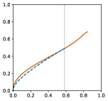
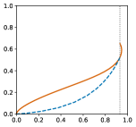
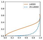
	ATPP	ATPP	ATPP

Figure 3.1: Comparison of AFDP-ATPP curve between LASSO and two-stage LASSO. Here we pick the setting $\delta=0.8$, $\epsilon=0.3$, $\sigma\in\{0.5,0.22,0.15\},p_{G}=\delta_{1}$. For two-stage LASSO, we use optimal tuning $\lambda^{*}_{1}$ in the first stage. All the curves are calculated based on Equations (2.2) and (2.5). The gray dotted line is the upper bound of ATPP that the two-stage LASSO can reach. Notice that even for LASSO, there is an upper bound which it cannot exceed.

Remark 3.1.

Theorems 3.1 and 3.2 prove that the optimal way to use two-stage variable selection is to set $\lambda=\lambda^{*}_{q}$ for the regularization parameter in the first stage. It is important to point out that $\lambda_{q}^{*}$ minimizes AMSE$(q,\lambda)$ and thus is the optimal tuning for parameter estimation. Therefore, the optimal tuning of the regularization parameter in bridge regression is the same for estimation and variable selection.

In the rest of the paper we will use the notation $s^{*}_{q}(\zeta)$ for the value of threshold that satisfies ${\rm ATPP}(q,\lambda^{*}_{q},s^{*}_{q}(\zeta))=\zeta$.

3.2 The best bridge estimator for variable selection

3.2.1 Summary

The two theorems we presented in the last section pave our way in addressing the question we raised in Section 1.1, i.e., finding the best bridge estimator based TVS technique. Consider $q_{1},q_{2}\in[1,\infty)$. We would like to compare ${\rm AFDP}(q_{1},\lambda^{*}_{q_{1}},s^{*}_{q_{1}}(\zeta))$ and ${\rm AFDP}(q_{2},\lambda^{*}_{q_{2}},s^{*}_{q_{2}}(\zeta))$. The following corollary of Theorems 3.1 and 3.2 shows the equivalence of the variable selection and estimation performance of bridge estimators.

Corollary 3.1.

Let $q_{1},q_{2}\geq 1$. If ${\rm AMSE}(q_{1},\lambda^{*}_{q_{1}})<{\rm AMSE}(q_{2},\lambda^{*}_{q_{2}})$, then for every $\zeta\in[0,1]$

$${\rm AFDP}(q_{1},\lambda^{*}_{q_{1}},s^{*}_{q_{1}}(\zeta))\leq{\rm AFDP}(q_{2},\lambda^{*}_{q_{2}},s^{*}_{q_{2}}(\zeta)).$$

The proof of this result is presented in Appendix D.3. According to Corollary 3.1, in order to see which two-stage method is better, we can compare their $\mathrm{AMSE}$ under optimal tuning $\lambda_{q}^{*}$. Such $\mathrm{AMSE}$ is given by (see Theorem B.1 and Lemma B.1 in the appendix)

$${\rm AMSE}(q,\lambda^{*}_{q})=\mathbb{E}\left(\eta_{q}(B+\tau_{*}Z;\alpha_{*}\tau_{*}^{2-q})-B\right)^{2},$$

where $\tau_{*}$ and $\alpha_{*}$ satisfy (2.3) and (2.4) with $\lambda=\lambda_{q}^{*}$.

The stage is finally set for comparing different two-stage variable selection techniques. Note that in the calculation of ${\rm AMSE}(q,\lambda^{*}_{q})$, the values of $\alpha_{*}$ and $\tau_{*}$ are required and can only be calculated through the fixed point equations (2.3) and (2.4). Therefore, we have no access to an explicit formula for ${\rm AMSE}(q,\lambda^{*}_{q})$. Furthermore, $\mathrm{AMSE}$ depends on many factors including $\delta$, $\sigma$ and $p_{B}$. This poses an extra challenge to completely evaluate and compare $\mathrm{AMSE}$ for different values of $q$. To address these issues, we focus on a few regimes that researchers have found useful in applications, and develop techniques to obtain explicit and accurate expressions for ${\rm AMSE}(q,\lambda^{*}_{q})$. These sharp results enable an accurate comparison among different TVS methods in each setting. The regimes we will consider are the following:

• Nearly black objects or rare signals: In this regime, $\epsilon$ is assumed to be small. In other words, there are very few non-zero coefficients that need to be detected. This model is called nearly black objects [DJHS92] or rare signals [DJ⁺15]. Intuitively speaking, it is also equivalent to the models considered in many other papers in which the sparsity level is assumed to be much smaller than the number of features. See for instance, [MB06, ZY06, ZH08] and the references therein. We will allow the signal strength to vary with respect to $\epsilon$. It turns out that the rate of signal strength affects the choice of optimal bridge estimator.

• Low SNR: In this model, $\sigma$ is considered to be large. This assumption is accurate in many social and medical studies. For more information, the reader may refer to [HTT17]. To explain the effect of SNR on the best choice of $q$, we will also mention a result for high SNR. Such assumption is also standard in the engineering applications, where the quality of measurements is carefully controlled. The analysis that is performed under the low noise setting is often called phase transition analysis, noise sensitivity analysis, or nearly exact recovery. See for instance [OH16, DT05, DMM11].

• Large sample regime: In this regime the per-feature sample size $\delta$ is large. This regime, as will be seen later, is closely related to the classical asymptotic regime $n/p\rightarrow\infty$, and is appropriate for traditional applied statistical problems. See for instance [KF00] for the asymptotic analysis of bridge estimators.

3.2.2 Analysis of AMSE for nearly black objects

As discussed in the preceding section, the formulas of $\mathrm{AMSE}$ are implicit and depend on $\delta$, $\sigma$ and $p_{B}$ in a complicated way. The goal of this section is to obtain explicit and accurate expressions for ${\rm AMSE}(q,\lambda_{q}^{*})$ when $\epsilon$ is small (i.e. the signal is very sparse). Towards this goal, a critical issue as made in e.g. [DJHS92] for the case of orthogonal design, is that the strength of the signal affects the performance of each estimator. Hence, in our analysis we let the strength of the signal vary with $\epsilon$. This generalization requires an extra notation we introduce here. Recall $G$ is the random variable with probability measure $p_{G}$, which determines the values of the non-zero entries of $\beta$. Define

$$b_{\epsilon}=\sqrt{\mathbb{E}G^{2}},\quad\tilde{G}=G/b_{\epsilon}.$$

Under this parameterization, $\mathbb{E}\tilde{G}^{2}=1$ and $b_{\epsilon}$ represents the (average) magnitude of each non-zero coefficient. We refer to $b_{\epsilon}$ as the signal strength and will allow it to change with the sparsity level $\epsilon$. Our first theorem characterizes the behavior of bridge estimators for $q>1$ and small values of $\epsilon$.

Theorem 3.3.

Suppose that $b_{\epsilon}\rightarrow\infty$ and $b_{\epsilon}=O(1/\sqrt{\epsilon})$. For $q>1$, we have

• If $b_{\epsilon}=\omega(\epsilon^{\frac{1-q}{2}})$, then

  $$\lim_{\epsilon\rightarrow 0}\epsilon^{-\frac{1}{q}}b_{\epsilon}^{-\frac{2(q-1)}{q}}\mathrm{AMSE}(q,\lambda_{q}^{*})=q(q-1)^{\frac{1}{q}-1}\sigma^{\frac{2}{q}}\big{[}\mathbb{E}|Z|^{\frac{2}{q-1}}\big{]}^{\frac{q-1}{q}}\big{[}\mathbb{E}|\tilde{G}|^{2q-2}\big{]}^{\frac{1}{q}}.$$

• If $b_{\epsilon}=o(\epsilon^{\frac{1-q}{2}})$, then $\lim_{\epsilon\rightarrow 0}\epsilon^{-1}b_{\epsilon}^{-2}{\rm AMSE}(q,\lambda_{q}^{*})=1$.

• If $\lim_{\epsilon\rightarrow 0}b_{\epsilon}\epsilon^{\frac{q-1}{2}}=c_{r}\in(0,\infty)$, then

  $$\lim_{\epsilon\rightarrow 0}\epsilon^{-\frac{1}{q}}b_{\epsilon}^{-\frac{2(q-1)}{q}}{\rm AMSE}(q,\lambda^{*}_{q})=\min_{C}h(C),$$

  where $h:\mathbb{R}^{+}\rightarrow\mathbb{R}$ and $h(C)\triangleq(Cq)^{-\frac{2}{q-1}}\sigma^{2}\mathbb{E}|Z|^{\frac{2}{q-1}}+\mathbb{E}\Big{(}\eta_{q}\big{(}c_{r}\tilde{G};C\sigma^{2-q}\big{)}-c_{r}\tilde{G}\Big{)}^{2}$. Furthermore, the minimizer of $h(C)$ is finite.

We note that when $q>2$, $b_{\epsilon}=o(\epsilon^{\frac{1-q}{2}})$ always holds, hence only the second item applies. When $q=2$, only the second and the thrid items apply.

This theorem is proved in Appendix E. Before we interpret this result, we characterize ${\rm AMSE}(1,\lambda_{1}^{*})$ in Theorem 3.4.

Theorem 3.4.

Suppose that $b_{\epsilon}\rightarrow\infty$ and $b_{\epsilon}=O(1/\sqrt{\epsilon})$. We have

• If $b_{\epsilon}=\omega(\sqrt{\log\epsilon^{-1}})$, then $\lim_{\epsilon\rightarrow 0}\frac{{\rm AMSE}(1,\lambda_{1}^{*})}{\epsilon\log\epsilon^{-1}}=2\sigma^{2}.$

• If $b_{\epsilon}=o(\sqrt{\log\epsilon^{-1}})$, then $\lim_{\epsilon\rightarrow 0}\frac{{\rm AMSE}(1,\lambda_{1}^{*})}{\epsilon b_{\epsilon}^{2}}=1$.

• If $\frac{b_{\epsilon}}{\sqrt{2\log\epsilon^{-1}}}\rightarrow c\in(0,\infty)$, then $\lim_{\epsilon\rightarrow 0}\frac{{\rm AMSE}(1,\lambda_{1}^{*})}{\epsilon\log\epsilon^{-1}}=\mathbb{E}(\eta_{1}(c\tilde{G};\sigma)-c\tilde{G})^{2}$.

This theorem will be proved in Appendix F. There are a few points that we should emphasize about Theorems 3.3 and 3.4.

Remark 3.2.

First let us discuss the assumptions of these two theorems. It is straightforward to show that with $b_{\epsilon}=\omega(1/\sqrt{\epsilon})$, the SNR per measurement goes to infinity. Such scenarios seem uncommon in applications, and for the sake of brevity we have only considered $b_{\epsilon}=O(1/\sqrt{\epsilon})$. Otherwise, the techniques we developed can be applied to higher SNR as well. Furthermore, we postpone the discussion about the case $b_{\epsilon}=O(1)$ to Theorem 3.5.

Remark 3.3.

The work of [DJHS92] has studied the problem of estimating an extremely sparse signal under the orthogonal design. The main goal of [DJHS92] is to obtain the minimax risk for the class of $\epsilon$-sparse signals (similar to our model) without any constraint on the signals’ power. They have shown that the approximately least favorable distribution has a point mass at $\Theta(\sqrt{\log(\epsilon^{-1})})$, and that LASSO achieves the minimax risk. Note that there are two major differences between Theorem 3.4 and the work of [DJHS92]: (i) our result is for non-orthogonal design, and (ii) we are not concerned with the minimax performance. In fact, we fix the power of the signal and obtain the asymptotic mean square error. This platform enables us to observe several delicate phenomena that are not observed in minimax settings. For instance, as is clear from Theorem 3.4, the rate of ${\rm AMSE}(1,\lambda_{1}^{*})$ undergoes a transition at the signal strength level $\Theta(\sqrt{\log(\epsilon^{-1})})$. As we will discuss later, below this threshold, LASSO is not necessarily optimal. However, since the risk of the Bayes estimator and LASSO is maximized for $b_{\epsilon}=\Theta(\sqrt{\log(\epsilon^{-1})})$, this important information is missed in minimax analysis.

Remark 3.4.

Compared to other bridge estimators, the performance of LASSO is much less sensitive to the strength of the signal: ${\rm AMSE}(1,\lambda_{1}^{*})\sim\epsilon\log\epsilon^{-1}$ as long as $b_{\epsilon}=\Omega(\sqrt{\log\epsilon^{-1}})$, while the order of ${\rm AMSE}(q,\lambda_{q}^{*})$ continuously changes as $b_{\epsilon}$ varies.

Theorems 3.3 and 3.4 can be used for comparing different bridge estimators, as clarified in our next corollary.

Corollary 3.2.

Suppose that $b_{\epsilon}=\epsilon^{-\gamma}$ for $\gamma\in(0,1/2]$. We have

• If $q>2\gamma+1$, then ${\rm AMSE}(q,\lambda_{q}^{*})\sim\epsilon^{1-2\gamma}$.

• If $1<q\leq 2\gamma+1$, then ${\rm AMSE}(q,\lambda_{q}^{*})\sim\epsilon^{\frac{1-2\gamma(q-1)}{q}}$.

• If $q=1$, then ${\rm AMSE}(q,\lambda_{q}^{*})\sim\epsilon\log(\epsilon^{-1})$.

The above result implies that in a wide range of signal strength, $q=1$ offers the smallest AMSE when the value of $\epsilon$ is very small. Consequently, according to Corollary 3.1, the two-stage LASSO provides the best variable selection performance. One can further confirm that the same conclusion continues to hold as long as $b_{\epsilon}=\omega(\sqrt{\log\epsilon^{-1}})$.

So far, we have seen that if the signal is reasonably strong, i.e. $b_{\epsilon}=\omega(\sqrt{\log\epsilon^{-1}})$, then two-stage LASSO outperforms all the other variable selection techniques. However, once $b_{\epsilon}=O(\sqrt{\log\epsilon^{-1}})$, we can see that ${\rm AMSE}(q,\lambda_{q}^{*})\sim\epsilon b_{\epsilon}^{2}$ for all $q\geq 1$. Hence, in order to provide a fair comparison, one should perform finer analyses and obtain a more accurate expression for $\mathrm{AMSE}$. Our next result shows how this can be done.

Theorem 3.5.

Consider $b_{\epsilon}=1$ and hence $\tilde{G}=G$. Assume $G$ is bounded from above. Then we have

$$\text{For }q=1: \quad\mathrm{AMSE}(1,\lambda_{1}^{*})=\epsilon\mathbb{E}G^{2}+o(\epsilon^{k}),\quad\forall k\in\mathbb{N};$$ (3.1)

$$\text{For }q>1: \quad\mathrm{AMSE}(q,\lambda^{*}_{q})=\epsilon\mathbb{E}G^{2}-\epsilon^{2}\frac{\mathbb{E}^{2}\Big{(}\big{|}\frac{G}{\sigma}+Z\big{|}^{\frac{1}{q-1}}\text{sgn}\big{(}\frac{G}{\sigma}+Z\big{)}G\Big{)}}{\mathbb{E}|Z|^{\frac{2}{q-1}}}+o(\epsilon^{2}),$$ (3.2)

where $\text{sgn}(\cdot)$ denotes the sign of a random variable.

The proof of this theorem is presented in Appendix G. The first interesting observation about this theorem is that, the first dominant term of $\mathrm{AMSE}$ is the same for all bridge estimators. The second dominant term, on the other hand, is much smaller for $q=1$ compared to the other values of $q$. Hence, LASSO is suboptimal in this setting. Accordingly, two-stage LASSO is outperformed by other TVS methods. However, as is clear from Theorem 3.5, we should not expect the bridge estimator with $q>1$ to outperform LASSO by a large margin when $\epsilon$ is too small. In fact, the second dominant term is proportional to $\epsilon^{2}$ (for $q>1$), while the first dominant term is proportional to $\epsilon$. Hence, the second dominant term is expected to become important for moderately small values of $\epsilon$. In such cases, we expect $q>1$ to offer more significant improvements. Regarding the optimal choice of $q$, it is determined by the constant of the second order term in (3.2). As is shown in Figure 3.2, while the optimal value of $q$ is case-dependent, it gets closer to 1 as the signal strength increases. This observation is consistent with the message delivered by Theorems 3.3 and 3.4.

	$M=1$	$M=2$	$M=3$
2nd order coef
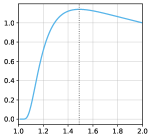
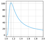
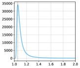
	$q$	$q$	$q$

Figure 3.2: The constant coefficient of the second order term in (3.2). We set $G=\delta_{M}$ with $M=1,2,3$ respectively and $\sigma=1$. As the signal strength $M$ increases, the optimal choice of $q$ shifts towards 1.

3.2.3 Analysis of AMSE in large noise scenario

This section aims to obtain explicit formulas for the optimal $\mathrm{AMSE}$ of bridge estimators in low SNR. This regime is particularly important, since in many social and medical studies, variable selection plays a key role and the SNR is low. The following theorem summarizes the main result of this section.

Theorem 3.6.

As $\sigma\rightarrow\infty$, we have the following expansions of AMSE$(q,\lambda_{q}^{*})$:

1. For $q=1$, when $G$ has a sub-Gaussian tail, we have

   $${\rm AMSE}(1,\lambda_{1}^{*})=\epsilon\mathbb{E}|G|^{2}+o(e^{-\frac{C^{2}\sigma^{2}}{2}}),$$ (3.3)

   where $C$ can be any positive number smaller than $C_{0}$, and $C_{0}>0$ is a constant only depending on $\epsilon$ and $G$. The explicit definition of $C_{0}$ can be found in the proof.

2. For $1<q\leq 2$, if all the moments of $G$ are finite, then

   $${\rm AMSE}(q,\lambda_{q}^{*})=\epsilon\mathbb{E}|G|^{2}-\frac{\epsilon^{2}(\mathbb{E}|G|^{2})^{2}c_{q}}{\sigma^{2}}+o(\sigma^{-2}),$$ (3.4)

   with $c_{q}=\frac{\big{(}\mathbb{E}|Z|^{\frac{2-q}{q-1}}\big{)}^{2}}{(q-1)^{2}\mathbb{E}|Z|^{\frac{2}{q-1}}}$.

3. For $q>2$, if $G$ has sub-Gaussian tail, then (3.4) holds.

We present our proofs in Appendix H. Figure 3.3 compares the accuracy of the first-order approximation and second-order approximation for moderate values of $\sigma$. As is clear, for $q\in(1,\infty)$, the second-order approximation provides an accurate approximation of ${\rm AMSE}(q,\lambda_{q}^{*})$ for a wide range of $\sigma$. Moreover, the first-order approximation for ${\rm AMSE}(1,\lambda_{1}^{*})$ is already accurate as can be justified by its exponentially small second order term in (3.3).

	$q=1$	$q=1.5$
relative error
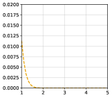
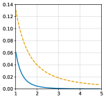
	$\sigma$	$\sigma$
	$q=2$	$q=2.5$
relative error
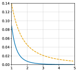
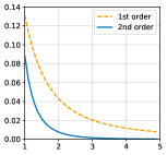
	$\sigma$	$\sigma$

Figure 3.3: Absolute relative error of first-order and second-order approximations of $\mathrm{AMSE}$ under large noise scenario. In these four figures, $p_{B}=(1-\epsilon)\delta_{0}+\epsilon\delta_{1}$, $\delta=0.4$, $\epsilon=0.2$.

According to this theorem, we can conclude that for sufficiently large $\sigma$, two-stage method with any $q>1$ can outperform the two-stage LASSO. This is because while the first dominant term is the same for all the bridge estimators with $q\in[1,\infty)$, the second order term for LASSO is exponentially smaller (in magnitude) than that of the other estimators. More interestingly, the following lemma shows that in fact $q=2$ leads to the smallest AMSE in the large noise regime.

$C_{q}$
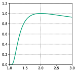
	$q$

Figure 3.4: The constant $c_{q}$ in Theorem 3.6 part (ii). The maximum is achieved at $q=2$.

Lemma 3.1.

The maximum of $c_{q}$, defined in Theorem 3.6, is achieved at $q=2$.

See Figure 3.4 for the plot of $c_{q}$.

Proof.

A simple integration by part yields:

$$\mathbb{E}|Z|^{\frac{2-q}{q-1}} = 2(q-1)\int_{0}^{\infty}z^{\frac{q}{q-1}}\phi(z)dz=(q-1)\mathbb{E}|Z|^{\frac{q}{q-1}}$$

We can then apply H$\ddot{o}$lders’s inequality to obtain

$$c_{q}=\frac{(\mathbb{E}|Z|^{\frac{q}{q-1}})^{2}}{\mathbb{E}|Z|^{\frac{2}{q-1}}}\leq\frac{\mathbb{E}|Z|^{\frac{2}{q-1}}\mathbb{E}Z^{2}}{\mathbb{E}|Z|^{\frac{2}{q-1}}}=1=c_{2}.$$

∎

Therefore, while the AMSE of all bridge estimators share the same first dominant term, Ridge offers the largest second dominant term (in magnitude), and hence the lowest AMSE. If we combine this result with Corollary 3.1, we conclude that in low SNR regime, two-stage Ridge obtains the best variable selection performance among TVS schemes with their first stage picked from the class of bridge estimators.

A comparison of this result with that for the high SNR derived in [WMZ⁺18] clarifies the impact of SNR on the best choice of $q$.

Theorem 3.7.

Assume $\epsilon\in(0,1)$. As $\sigma\rightarrow 0$, we have the following expansions of AMSE$(q,\lambda_{q}^{*})$ in terms of $\sigma$.

1. For $q=1$, if $\mathbb{P}(|G|\geq\mu)=1$ for some $\mu>0$, $\delta>M_{1}(\epsilon)$, and $\mathbb{E}|G|^{2}<\infty$, then

   $${\rm AMSE}(1,\lambda_{1}^{*})=\frac{\delta M_{1}(\epsilon)}{\delta-M_{1}(\epsilon)}\sigma^{2}+o\big{(}e^{\frac{(M_{1}(\epsilon)-\delta)\tilde{\mu}^{2}}{2\delta\sigma^{2}}}\big{)},$$ (3.5)

   where $M_{1}(\epsilon)=\min_{\chi}(1-\epsilon)\mathbb{E}\eta_{1}^{2}(Z;\chi)+\epsilon(1+\chi^{2})$, and $\tilde{\mu}$ can be any positive number smaller than $\mu$.

2. For $1<q<2$, if $\mathbb{P}(|G|\leq x)=O(x)$ (as $x\rightarrow 0$), $\delta>1$, and $\mathbb{E}|G|^{2}<\infty$ then

   $${\rm AMSE}(q,\lambda_{q}^{*})=\frac{\sigma^{2}}{1-1/\delta}-\sigma^{2q}\frac{\delta^{q+1}(1-\epsilon)^{2}(\mathbb{E}|Z|^{q})^{2}}{(\delta-1)^{q+1}\epsilon\mathbb{E}|G|^{2q-2}}+o(\sigma^{2q}).$$ (3.6)

3. For $q=2$, if $\delta>1$ and $\mathbb{E}|G|^{2}<\infty$, we have

   $${\rm AMSE}(2,\lambda_{2}^{*})=\frac{\sigma^{2}}{1-1/\delta}-\sigma^{4}\frac{\delta^{3}}{(\delta-1)^{3}\epsilon\mathbb{E}|G|^{2}}+o(\sigma^{4}).$$ (3.7)

4. For $q>2$, if $\delta>1$ and $\mathbb{E}|G|^{2q-2}<\infty$, then

   $${\rm AMSE}(q,\lambda_{q}^{*})=\frac{\sigma^{2}}{1-1/\delta}-\sigma^{4}\frac{\delta^{3}\epsilon(q-1)^{2}(\mathbb{E}|G|^{q-2})^{2}}{(\delta-1)^{3}\mathbb{E}|G|^{2q-2}}+o(\sigma^{4}).$$ (3.8)

The results for $q\in[1,2]$ are taken from [WMZ⁺18]. The proof for the case $q>2$ can be found in Appendix I of [WWM17]. It is straightforward to see that $M_{1}(\epsilon)$ is an increasing function of $\epsilon\in[0,1]$ and $M_{1}(1)=1$. This implies that ${\rm AMSE}(1,\lambda_{1}^{*})$ is the smallest among all ${\rm AMSE}(q,\lambda_{q}^{*})$ with $q\in[1,\infty)$. As is clear, the first order terms in the expansion of ${\rm AMSE}(q,\lambda_{q}^{*})$ are the same for all $q\in(1,\infty)$. However, the second dominant term shows that the smaller values of $q$ are preferable (note the strict monotonicity only occurs in the range $(1,2]$).

Combining the above results with Corollary 3.1 implies that in the high SNR setting, two-stage LASSO offers the best variable selection performance. We should also emphasize that as depicted in Figure 3.1, in this regime two-stage LASSO offers a much better variable selection performance than LASSO.

Remark 3.5.

Theorems 3.6 and 3.7 together give a full and sharp evaluation of the noise-sensitivity of bridge estimators. Among all the bridge estimators with $q\in[1,\infty)$, LASSO and Ridge are optimal for parameter estimation and variable selection, in the low and large noise settings respectively. This result delivers an intriguing message: sparsity inducing regularization is not necessarily preferable even in sparse models. Such phenomenon might be well explained by the bias-variance tradeoff: variance is the major factor in very noisy settings, thus a regularization that produces more stable estimator is preferred, when the noise is large.

3.2.4 Analysis of AMSE in large sample scenario

Our analysis in this section is concerned with the large $\delta$ regime. Since $n/p\rightarrow\delta$ in our asymptotic setting, large $\delta$ means large sample size (relative to the dimension $p$). Intuitively speaking, this is similar to the classical asymptotic setting where $n\rightarrow\infty$ and $p$ is fixed (specially if we assume the fixed number $p$ is large). We will later connect the results we derive in the large $\delta$ regime to those obtained in classical asymptotic regime, and provide new insights.

In our original set-up, the elements of the design matrix are $X_{ij}\overset{i.i.d.}{\sim}N(0,\frac{1}{n})$. This means the SNR ${\rm var}(\sum_{j}X_{ij}\beta_{j})/{\rm var}(w_{i})\rightarrow\frac{\mathbb{E}|B|^{2}}{\delta\sigma^{2}}$ as $n\rightarrow\infty$. Therefore, if we let $\delta\rightarrow\infty$, the SNR will decrease to zero, which is not consistent with the classical asymptotics in which the SNR is assumed to be fixed. To resolve this discrepancy we scale the noise term by $\sqrt{\delta}$ and use the model:

$$y=X\beta+\frac{1}{\sqrt{\delta}}w,$$ (3.9)

where $\{\beta,w,X\}$ is the converging sequence in Definition 2.1. Under this model we compare the AMSE of different bridge estimators. The next theorem summarizes the main result.

Theorem 3.8.

Consider the model in (3.9) and $\epsilon\in(0,1)$. As $\delta\rightarrow\infty$, we have

1. For $q=1$, if $\mathbb{P}(|G|\geq\mu)=1$ for some $\mu>0$ and $\mathbb{E}|G|^{2}<\infty$, then

   $${\rm AMSE}(1,\lambda^{*}_{1})=\frac{M_{1}(\epsilon)\sigma^{2}}{\delta}+o(\delta^{-1}),$$ (3.10)

   where $M_{1}(\epsilon)$ has the same definition as in Theorem 3.7 (i).

2. For $1<q<2$, if $\mathbb{P}(|G|\leq x)=O(x)$ (as $x\rightarrow 0$) and $\mathbb{E}|G|^{2}<\infty$, then

   $${\rm AMSE}(q,\lambda^{*}_{q})=\frac{\sigma^{2}}{\delta}-\frac{\sigma^{2q}}{\delta^{q}}\frac{(1-\epsilon)^{2}(\mathbb{E}|Z|^{q})^{2}}{\epsilon\mathbb{E}|G|^{2q-2}}+o\big{(}\delta^{-q}\big{)}$$ (3.11)

3. For $q=2$, if $\mathbb{E}|G|^{2}<\infty$, then we have

   $${\rm AMSE}(2,\lambda^{*}_{2})=\frac{\sigma^{2}}{\delta}+\frac{\sigma^{2}}{\delta^{2}}\big{[}1-\frac{\sigma^{2}}{\epsilon\mathbb{E}G^{2}}\big{]}+o(\delta^{-2})$$ (3.12)

4. For $q>2$, if $\mathbb{E}|G|^{2q-2}<\infty$, then

   $${\rm AMSE}(q,\lambda^{*}_{q})=\frac{\sigma^{2}}{\delta}+\frac{\sigma^{2}}{\delta^{2}}\bigg{[}1-\frac{\epsilon(q-1)^{2}\sigma^{2}(\mathbb{E}|G|^{q-2})^{2}}{\mathbb{E}|G|^{2q-2}}\bigg{]}+o(\delta^{-2}).$$ (3.13)

The proof of Theorem 3.8 can be found in Appendix I. Figure 3.5 compares the accuracy of the first and second order expansions in large range of $\delta$. As is clear from this figure, the second-order term often offers an accurate approximation over a wide range of $\delta$.

Remark 3.6.

As mentioned in Section 3.2.3, $M_{1}(\epsilon)$ is an increasing function of $\epsilon\in[0,1]$ and $M_{1}(1)=1$. This implies that ${\rm AMSE}(1,\lambda_{1}^{*})$ is the smallest among all ${\rm AMSE}(q,\lambda_{q}^{*})$ with $q\in[1,\infty)$. Therefore, in this regime LASSO gives the smallest estimation error and thus two-stage LASSO offers the best variable selection performance.

Remark 3.7.

The ${\rm AMSE}(q,\lambda_{q}^{*})$ with $q>1$ share the same first dominant term, but have different second order terms. Furthermore, for $q\in(1,2]$, the smaller $q$ is, the better its performance will be. Such monotonicity does not hold beyond $q=2$.

	$q=1$	$q=1.5$
relative error
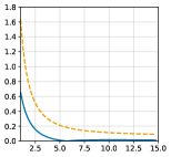
	$\delta$	$\delta$
	$q=2$	$q=2.5$
relative error
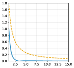
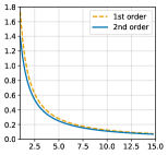
	$\delta$	$\delta$

Figure 3.5: Absolute relative error of first-order and second-order approximations of AMSE under large sample scenario. In these four figures, $p_{B}=(1-\epsilon)\delta_{0}+\epsilon\delta_{1}$, $\epsilon=0.5$, $\sigma=1$.

We now connect our results in this large $\delta$ regime to those obtained in classical asymptotic setting. The classical aymptotics ($p$ fixed) of bridge estimators for all the values of $q\in[0,\infty)$ is studied in [KF00]. We explain LASSO first. According to [KF00], if $\frac{\lambda}{\sqrt{n}}\rightarrow\lambda_{0}\geq 0$ and $\frac{1}{n}X^{T}X\rightarrow C$, then

$$\sqrt{n}(\hat{\beta}-\beta)\xrightarrow{d}\arg\min_{u}V(u),$$ (3.14)

where $V(u)=-2u^{T}W+u^{T}Cu+\lambda_{0}\sum_{j=1}^{p}[u_{j}\text{sgn}(\beta_{j})\mathbbm{1}_{\{\beta_{j}\neq 0\}}+|u_{j}|\mathbbm{1}_{\{\beta_{j}=0\}}]$ with $W\sim\mathcal{N}(0,\sigma^{2}C)$. We will do the following calculations to explore the connections. Since $X_{ij}\sim N(0,1/n)$ in our paper, we first make the following changes to LASSO to make our set-up consistent with that of [KF00]:

$$\frac{1}{2}\|y-X\beta\|_{2}^{2}+\lambda\|\beta\|_{1}=\frac{1}{2}\Big{(}\|y-\sqrt{n}X\frac{\beta}{\sqrt{n}}\|_{2}^{2}+2\sqrt{n}\lambda\|\frac{\beta}{\sqrt{n}}\|_{1}\Big{)}.$$

We thus have $C=\frac{1}{n}(\sqrt{n}X)^{T}(\sqrt{n}X)\rightarrow I$ and $\lambda_{0}=2\lambda$. Now suppose the result (3.14) works for $\hat{\beta}(1,\lambda)$. Then we have

$$\hat{\beta}(1,\lambda)-\beta\xrightarrow{d}\arg\min_{u}V(u),$$ (3.15)

where $V(u)=-2u^{T}W+u^{T}u+2\lambda\sum_{j=1}^{p}[u_{j}\text{sgn}(\beta_{j})\mathbbm{1}_{\{\beta_{j}\neq 0\}}+|u_{j}|\mathbbm{1}_{\{\beta_{j}=0\}}]$ with $W\sim\mathcal{N}(0,\frac{\sigma^{2}}{\delta}I)$. It is straightforward to see that the optimal choice of $u$ in (3.15) has the following form:

$$\hat{u}_{j}=\left\{\begin{array}[]{ll}W_{j}-\lambda\text{sgn}(\beta_{j})&\text{ when }\beta_{j}\neq 0\\ W_{j}-\lambda s(\hat{u}_{j})&\text{ when }\beta_{j}=0\end{array}\right.$$

where $s(u_{j})=\text{sgn}(u_{j})$ when $u_{j}\neq 0$ and $|s(u_{j})|\leq 1$ when $u_{j}=0$. Furthermore, for the case of $\beta_{j}=0$, $\hat{u}_{j}=0$ is equivalent to $|W_{j}|\leq\lambda$ and $\text{sgn}(W_{j})=\text{sgn}(\hat{u}_{j})$ when $\hat{u}_{j}\neq 0$. Based on this result, we do the following heuristic calculation to connect our results with those of [KF00]:

$$\frac{1}{p}\|\hat{\beta}(1,\lambda)-\beta\|_{2}^{2}\approx \frac{1}{p}\mathbb{E}\bigg{[}\sum_{j:\beta_{j}\neq 0}\big{[}W_{j}^{2}-2\lambda\text{sgn}(\beta_{j})W_{j}+\lambda^{2}\big{]}+\sum_{j:\beta_{j}=0,\hat{u}_{j}\neq 0}\big{[}W_{j}^{2}-2\lambda W_{j}\text{sgn}(\hat{u}_{j})+\lambda^{2}\big{]}\bigg{]}$$

$$\approx \frac{1}{p}\bigg{[}\sum_{j:\beta_{j}\neq 0}(\frac{\sigma^{2}}{\delta}+\lambda^{2})+\sum_{j:\beta_{j}=0}\mathbb{E}\eta_{1}^{2}(W_{j};\lambda)\bigg{]}=\frac{k}{p}(\frac{\sigma^{2}}{\delta}+\lambda^{2})+\frac{p-k}{p}\mathbb{E}\eta_{1}^{2}(W_{j};\lambda)$$

$$= \frac{\sigma^{2}}{\delta}\Big{[}\frac{p-k}{p}\mathbb{E}\eta^{2}_{1}(Z;\sqrt{\delta}\lambda/\sigma)+\frac{k}{p}(1+(\sqrt{\delta}\lambda/\sigma)^{2})\Big{]},$$

where $k$ is the number of non-zero elements of $\beta$ and $Z\sim N(0,1)$. Note that in our asymptotic setting $k/p\rightarrow\epsilon$ and we consider the optimal tuning $\lambda_{1}^{*}$. Therefore following the above calculations we obtain

$$\min_{\lambda}\frac{1}{p}\|\hat{\beta}(1,\lambda)-\beta\|_{2}^{2}\approx\frac{\sigma^{2}}{\delta}\min_{\chi}(1-\epsilon)\mathbb{E}\eta_{1}^{2}(Z;\chi)+\epsilon(1+\chi^{2})=\frac{M_{1}(\epsilon)\sigma^{2}}{\delta}.$$

This is consistent with (3.10) in our asymptotic analysis. We can do similar calculations to show that the asumptotic analysis of [KF00] leads to the first order expansion of AMSE in Theorem 3.8 for the case $q>1$.

Based on this heuristic argument, we may conclude that the information provided by the classical asymptotic analysis is reflected in the first order term of AMSE$(q,\lambda_{q}^{*})$. Moreover, our large sample analysis is able to derive the second dominant term for $q>1$. This term enables us to compare the performance of different values of $q>1$ more accurately (note they all have the same first order term). Such comparisons cannot be performed in [KF00].

4 Debiasing

4.1 Implications of debiasing for LASSO

As is clear from Theorem 3.2, since LASSO produces a sparse solution, it is not possible for a LASSO based two-stage method to achieve ATPP values beyond what is already reached by the first stage. This problem can be resolved by debiasing. In this approach, instead of thresholding the LASSO estimate (or in general a bridge estimate), we threshold its debiased version. Below we will add a dagger $\dagger$ to aforementioned notations to denote their corresponding debiased version. Recall $\hat{\beta}(q,\lambda)$ denotes the solution of bridge regression for any $q\geq 1$. Define the debiased estimates as

1. For $q=1$,

   $$\hat{\beta}^{\dagger}(1,\lambda)\triangleq\hat{\beta}(1,\lambda)+X^{T}\frac{y-X\hat{\beta}(1,\lambda)}{1-\|\hat{\beta}(1,\lambda)\|_{0}/n},$$

   where $\|\cdot\|_{0}$ counts the number of non-zero elements in a vector.

2. For $q>1$,

   $$\hat{\beta}^{\dagger}(q,\lambda)\triangleq\hat{\beta}(q,\lambda)+X^{T}\frac{y-X\hat{\beta}(q,\lambda)}{1-f(\hat{\beta}(q,\lambda),\hat{\gamma}_{\lambda})/n},$$ (4.1)

   where $f(v,w)=\sum_{i=1}^{p}\frac{1}{1+wq(q-1)|v_{i}|^{q-2}}$ and $\gamma=\hat{\gamma}_{\lambda}$ is the unique solution of the following equation:

   $$\frac{\lambda}{\gamma}=1-\frac{1}{n}f(\hat{\beta}(q,\lambda),\gamma).$$ (4.2)

We have the following theorem to confirm the validity of the debiasing estimator $\hat{\beta}^{\dagger}(q,\lambda)$.

Theorem 4.1.

For any given $q\in[1,\infty)$, with probability one, the empirical distribution of the components of $\hat{\beta}^{\dagger}(q,\lambda)-\beta$ converges weakly to $N(0,\tau^{2})$, where $\tau$ is the solution of (2.3) and (2.4).

See Appendix J for the proof. In order to perform variable selection, one may apply the hard thresholding function to these debiased estimates, i.e.,

$$\bar{\beta}^{\dagger}(q,\lambda,s)=\eta_{0}(\hat{\beta}^{\dagger}(q,\lambda);s^{2}/2)=\hat{\beta}^{\dagger}(q,\lambda)\mathbbm{1}_{\{|\hat{\beta}^{\dagger}(q,\lambda)|\geq s\}}.$$

We use the notations ${\rm ATPP}^{\dagger}(q,\lambda,s)$ and ${\rm AFDP}^{\dagger}(q,\lambda,s)$ to denote the ATPP and AFDP of $\bar{\beta}^{\dagger}(q,\lambda,s)$ respectively. In the case of LASSO, note that unlike $\hat{\beta}(1,\lambda)$ the debiased estimator $\hat{\beta}^{\dagger}(1,\lambda)$ is dense. Hence we expect the two-stage variable selection estimate $\bar{\beta}^{\dagger}(1,\lambda,s)$ to be able to reach any value of ATPP between $[0,1]$. The following theorem confirms this claim.

Theorem 4.2.

Given the ATPP level $\zeta\in[0,1]$, for every value of $\lambda>0$, there exists $s(\lambda,\zeta)$ such that ${\rm ATPP}^{\dagger}(1,\lambda,s(\lambda,\zeta))=\zeta$. Furthermore, whenever $\bar{\beta}^{\dagger}(1,\lambda,s)$ and $\bar{\beta}(1,\lambda,\tilde{s})$ reach the same level of ATPP, they have the same AFDP. The value of $\lambda$ that minimizes ${\rm AFDP}^{\dagger}(1,\lambda,s(\lambda,\zeta))$ also minimizes ${\rm AMSE}(1,\lambda)$.

As expected since the solution of bridge regression for $q>1$ is dense, the debiasing step does not help variable selection for $q>1$. Our next theorem confirms this claim.

Theorem 4.3.

Consider $q>1$. Given the ATPP level $\zeta\in[0,1]$, for every value of $\lambda>0$, there exists $s(\lambda,\zeta)$ such that ${\rm ATPP}^{\dagger}(q,\lambda,s(\lambda,\zeta))=\zeta$. Furthermore, whenever $\bar{\beta}^{\dagger}(q,\lambda,s)$ and $\bar{\beta}(q,\lambda,\tilde{s})$ reach the same level of ATPP, they have the same AFDP. Also, the value of $\lambda$ that minimizes ${\rm AFDP}^{\dagger}(q,\lambda,s(\lambda,\zeta))$ also minimizes ${\rm AMSE}(q,\lambda)$. As a result, the optimal value of ${\rm AFDP}^{\dagger}(q,\lambda,s(\lambda,\zeta))$ is the same as ${\rm AFDP}(q,\lambda^{*}_{q},s^{*}_{q}(\zeta))$.

For the proof of Theorems 4.2 and 4.3, please refer to Appendix J.

Remark 4.1.

Comparing Theorem 4.2 with Theorem 3.2, we see that replacing LASSO in the first stage with the debiased version enables to achieve wider range of ATPP level. On the other hand, given the value of $\lambda$, if $\bar{\beta}^{\dagger}(1,\lambda,s)$ and $\bar{\beta}(1,\lambda,\tilde{s})$ reach the same level of ATPP, their AFDP are equal as well. Therefore, the debiasing for LASSO expands the range of AFDP-ATPP curve without changing the original one. Figure 4.1 compares the variable selection performance of LASSO with that of the two-stage scheme having the debiased LASSO estimate in the first stage. Compare this figure with Figure 3.1 to see the difference between the two-stage LASSO and two-stage debiased LASSO.

	$\sigma=0.5$	$\sigma=0.22$	$\sigma=0.15$
AFDP
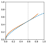
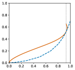
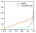
	ATPP	ATPP	ATPP

Figure 4.1: Comparison of AFDP-ATPP curve between LASSO and two-stage debiased LASSO. Here we pick the setting $\delta=0.8$, $\epsilon=0.3$, $\sigma\in\{0.5,0.22,0.15\},p_{G}=\delta_{1}$. For the two-stage debiased LASSO, we use optimal tuning $\lambda_{1}^{*}$ in the first stage. The gray dotted line is the upper bound for the two-stage LASSO without debiasing can reach.

Remark 4.2.

The debiasing does not present any extra gain to the two-stage variable selection technique based on bridge estimators with $q>1$. In other words, debiasing does not change the AFDP-ATPP curve for $q>1$.

4.2 Debiasing and Sure Independence Screening

Sure Independence Screening (SIS) is a variable selection scheme proposed for ultra-high dimensional settings [FL08]. Our asymptotic setting is not considered an ultra-high dimensional asymptotic. We are also aware that SIS is typically used for screening out irrelevant variables and other variable selection methods, such as LASSO, will be applied afterwards. Nevertheless, we present a connection and comparison between our two-stage methods and SIS in the linear asymptotic regime. Such comparisons shed more light on the performance of SIS. It is straightforward to confirm that Sure Independence Screening is equivalent to

$$\bar{\beta}^{\dagger}(q,\infty,s)=\eta_{0}(\hat{\beta}^{\dagger}(q,\infty);s^{2}/2)=\eta_{0}(X^{T}y;s^{2}/2).$$

Therefore, the main difference between the approach we propose in this paper and SIS, is that SIS sets $\lambda$ to $\infty$, while we select the value of $\lambda$ that minimizes AMSE. This simple difference may give a major boost to the variable selection performance. The following lemma confirms this claim.

	$\sigma=0.5$	$\sigma=0.22$	$\sigma=0.15$
AFDP
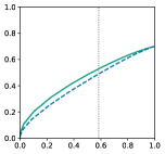
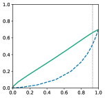
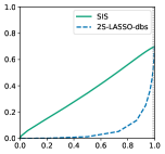
	ATPP	ATPP	ATPP

Figure 4.2: Comparison of AFDP-ATPP curve between SIS and the two-stage debiased LASSO. Here we pick the setting $\delta=0.8$, $\epsilon=0.3$, $\sigma\in\{0.5,0.22,0.15\},p_{G}=\delta_{1}$. For the two-stage debiased LASSO, we use optimal tuning $\lambda^{*}_{1}$ in the first stage. The gray dotted line is the upper bound that the two-stage LASSO without debiasing can reach.

Lemma 4.1.

Consider $q\geq 1$. Given any ATPP level $\zeta\in[0,1]$, let ${\rm AFDP}_{\rm sis}(\zeta)$ and ${\rm AFDP}^{\dagger}(q,\lambda_{q}^{*},s(\lambda_{q}^{*},\zeta))$ denote the asymptotic FDP of SIS and two-stage debiased bridge estimator respectively, when their ATPP is equal to $\zeta$. Then, ${\rm AFDP}^{\dagger}(q,\lambda^{*}_{q},s(\lambda^{*}_{q},\zeta))\leq{\rm AFDP}_{\rm sis}(\zeta)$.

Refer to Appendix J for the proof. Note that when the noise $\sigma$ is large, we expect the optimally tuned $\lambda$ to be large, and hence the performance of SIS gets closer to the TVS. However, as $\sigma$ decreases, the gain obtained from using a better estimator in the first stage improves. Figure 4.2 compares the performance of SIS and TVS under different noise settings.

5 Numerical experiments

5.1 Objective and Simulation Set-up

This section aims to investigate the finite sample performances of various two-stage variable selection estimators under the three different regimes analyzed in Section 3.2. In particular, we will study to what extent our theory works for more realistic situations, where model parameters $\sigma$, $\epsilon$, $\delta$ are of moderate magnitudes or the iid-Gaussian design assumption is violated. For brevity, we will use bridge estimator to refer to the corresponding two-stage method whenever it does not cause any confusion. More specifically, in all the figures, $\ell_{q}$ will be used to denote the TVS that uses the bridge estimator with $q$ in the first stage, and $\ell_{1}$-db denotes the two-stage debiased LASSO. The performances of different methods will be compared via the AFDP-ATPP curves.

The organization of this section is as follows. In Sections 5.2 - 5.6, we focus on experiments under iid-Gaussian design as assumed in our theories. In Section 5.7, we present numerical results for non-i.i.d. or non-Gaussian designs to evaluate the accuracy of our results, when i.i.d. Gaussian assumption on $X$ is violated.

We adopt the following settings for iid-Gaussian design. The settings for general design are described in Section 5.7.

1. Number of variables is fixed at $p=5000$. Sample size $n=p\delta$ is then decided by $\delta$.

2. Given the values of $\delta$, $\epsilon$, $\sigma$, we sample $X\in\mathbb{R}^{n\times p}$ with $X_{ij}\overset{i.i.d.}{\sim}\mathcal{N}(0,\frac{1}{n})$. We pick the probability measure $p_{G}$ as a point mass at $M$ where $M$ will be specified in each scenario. We generate $\beta\in\mathbb{R}^{p}$ with $\beta_{i}\overset{i.i.d.}{\sim}p_{B}=(1-\epsilon)\delta_{0}+\epsilon p_{G}$, and $w\in\mathbb{R}^{n}$ with $w_{i}\overset{i.i.d.}{\sim}\mathcal{N}(0,\sigma^{2})$ or $\mathcal{N}(0,\frac{\sigma^{2}}{\delta}).$ Construct $y$ according to $y=X\beta+w$.

3. For each data set $(y,X)$, AFDP-ATPP curves will be generated for different variable selection methods. In each setting of parameters, 80 samples are drawn and the average AFDP-ATPP curves are calculated. The associated one standard deviation confidence interval will be presented.

We compute bridge estimators via coordinate descent algorithm, with the proximal operator $\eta_{q}(x;\tau)$ calculated through a properly implemented Newton’s method.

We discuss how to pick optimal tuning under iid-Gaussian design in Section 5.2. Section 5.3 presents the large/small noise scenario. Section 5.4 is devoted to the large sample regime. Section 5.5 covers the nearly black object scenario. In Section 5.6, we compare the performance of LASSO and two-stage LASSO to shed more lights on our two-stage methods.

5.2 Estimating the optimal tuning $\lambda_{q}^{*}$

For two-stage variable selection procedures, it is critical to have a good estimator in the first step. One challenge here is to search for the optimal tuning that minimizes $\mathrm{AMSE}$ of $\hat{\beta}(q,\lambda)$. According to the result of Theorem B.1 and the definition of ${\rm AMSE}$ in (2.1), it is straightforward to see that $\tau^{2}=\sigma^{2}+\frac{1}{\delta}\mathrm{AMSE}$. Hence, one can minimize $\tau^{2}$ to achieve the same optimal tuning. Motivated by [MMB⁺18], we can obtain a consistent estimator of $\tau^{2}$:

$$q=1:\quad\hat{\tau}^{2}=\frac{\|y-X\hat{\beta}(1,\lambda)\|_{2}^{2}}{n(1-\|\hat{\beta}(1,\lambda)\|_{0}/n)^{2}},\qquad q>1:\quad\hat{\tau}^{2}=\frac{\|y-X\hat{\beta}(q,\lambda)\|_{2}^{2}}{n(1-f(\hat{\beta}(q,\lambda),\hat{\gamma}_{\lambda})/n)^{2}},$$

where $f(\cdot,\cdot),\hat{\gamma}_{\lambda}$ are the same as the ones in (4.1) and (4.2). The consistency $\hat{\tau}\overset{a.s.}{\rightarrow}\tau$ can be easily seen from the proof of Theorem 4.1. We thus do not repeat it. As a result, we approximate $\lambda_{q}^{*}$ by searching for the $\lambda$ that minimizes $\hat{\tau}^{2}$. Notice that this problem has been studied for LASSO in [MMB⁺18] and a generalization is straightforward for other bridge estimators. We use the following grid search strategy:

• Initialization: An initial search region $[a,b]$, a window size $\Delta$ and a grid size $m$.

• Searching: A grid with size $m$ is built over $[a,b]$, upon which we search in descending order for $\lambda$ that minimizes $\hat{\tau}^{2}$ with warm initialization.

  • If the minimal point $\hat{\lambda}\in(a,b)$, stop searching and return $\hat{\lambda}$.

  • If $\hat{\lambda}=a$ or $b$, update the search region with $[\frac{a}{10},a]$ or $[b,b+\Delta]$ and do the next round of searching.

• Stability: If the optimal $\hat{\lambda}$ obtained from two consecutive search regions are smaller than a threshold $\epsilon_{0}$, we stop and return the previous optimal $\hat{\lambda}$; If the number of non-zero locations of a LASSO estimator is larger than $n$ (which may happen numerically for very small tuning), we set its $\hat{\tau}^{2}$ to $\infty$.

For our experiments, we pick the initial $[a,b]=[0.1,\frac{1}{2}\|X^{T}y\|_{\infty}]$, $\Delta=\frac{1}{2}\|X^{T}y\|_{\infty}$ and $m=15$.

5.3 From large noise to small noise

Theorems 3.6 and 3.7 showed that in low and high SNR situations, ridge and LASSO offer the best performances respectively. These results are obtained for limiting cases $\sigma\rightarrow\infty$ and $\sigma\rightarrow 0$. In this section, we run a few simulations to clarify the scope of applicability of our analysis. Toward this goal, we fix the probability measure $p_{G}=\delta_{M}$ with $M=8$ and run TVS for $q\in\{1,1.2,2,4\}$ and debiased LASSO under four settings:

1. $\delta=0.8$, $\epsilon=0.2$: The results are shown in Figure 5.1. Here we pick $\sigma\in\{1.5,3,5\}$. As expected from our theoretical results, for small values of noise LASSO offers the best performance. As we increase the noise, eventually ridge outperforms LASSO and the other bridge estimators. Note that under this setting, the outperformance occurs at a high noise level so that all estimators have large errors. In this example, we make $1>\delta>M_{1}(\epsilon)$. Refer to Theorem 3.7 for the importance of this condition.

   	$\sigma=1.5$	$\sigma=3$	$\sigma=5$
   AFDP
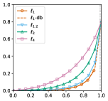
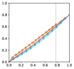
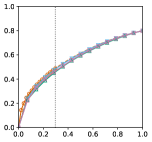
   	ATPP	ATPP	ATPP
   $\mathrm{AFDP}_{q}-\mathrm{AFDP}_{2}$
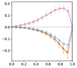
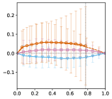
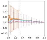
   	ATPP	ATPP	ATPP
   	$\sigma=2$	$\sigma=4$	$\sigma=8$
   AFDP
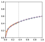
   	ATPP	ATPP	ATPP
   $\mathrm{AFDP}_{q}-\mathrm{AFDP}_{2}$
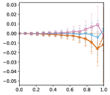
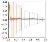
   	ATPP	ATPP	ATPP

   Figure 5.1: Top row: AFDP-ATPP curve under the setting $\delta=0.8$, $\epsilon=0.2,\sigma\in\{1.5,3,5\}$. Second row: Y-axis is the difference of AFDP between the other bridge estimators and ridge. One standard deviation of the difference is added. Third and fourth rows: the same type of plots as in the first two rows, under the setting $\delta=2$, $\epsilon=0.4,\sigma\in\{2,4,8\}$.

   	$\sigma=0.25$	$\sigma=0.75$	$\sigma=2$
   AFDP
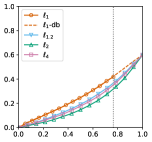
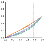
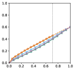
   	ATPP	ATPP	ATPP
   $\mathrm{AFDP}_{q}-\mathrm{AFDP}_{2}$
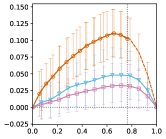
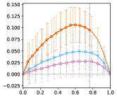
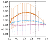
   	ATPP	ATPP	ATPP
   	$\sigma=1.2$	$\sigma=1.5$	$\sigma=1.9$
   AFDP
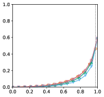
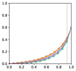
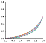
   	ATPP	ATPP	ATPP
   $\mathrm{AFDP}_{q}-\mathrm{AFDP}_{2}$
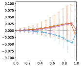
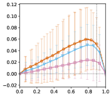
   	ATPP	ATPP	ATPP

   Figure 5.2: Top row: AFDP-ATPP curve under the setting $\delta=0.6$, $\epsilon=0.4,\sigma\in\{0.25,0.75,2\}$. Second row: Y-axis is the difference of AFDP between the other bridge estimators and ridge. One standard deviation of the difference is added. Third and fourth rows: the same type of plots as in the first two rows, under the setting $\delta=0.9$, $\epsilon=0.4,\sigma\in\{1.2,1.5,1.9\}$.

2. $\delta=2$, $\epsilon=0.4$: The results are included in Figure 5.1. Here we pick $\sigma\in\{2,4,8\}$. Similar phenomena are observed. However for all choices of $\sigma$, the AFDP-ATPP curves of different methods are quite close to each other.

3. $\delta=0.6$, $\epsilon=0.4$: Figure 5.2 contains the results for this part. Here we have $\sigma\in\{0.25,0.75,2\}$. An important feature of this simulation is that $\delta<M_{1}(\epsilon)$, which does not satisfy the condition of Theorem 3.7. It is interesting to observe that in this case, ridge outperforms LASSO even for small values of the noise. We thus see that the superiority of LASSO in small noise characterized by Theorem 3.7 may not hold when the conditions of the theorem are violated. In fact, Theorem 3.7 is restricted to the regime below the phase transition (i.e., when the signal can be fully recovered without noise). However, in the current setting, the optimal $\mathrm{AMSE}$ for $q=1,1.2,2,4$ at $\sigma=0$ are $14.9,12.2,10.2,11.6$, respectively.

4. $\delta=0.9$, $\epsilon=0.4$: The results are shown in Figure 5.2. Here we have $\sigma\in\{1.2,1.5,1.9\}$. This group of figures provide us with examples where ridge based TVS outperforms the other two-stage methods, and at the same time reaches a quite satisfactory AFDP-ATPP trade-off. For instance, when $\sigma=1.5$ and $\text{AFDP}\approx 0.2$, for ridge we have $\text{ATPP}\approx 0.8$ while that for LASSO is around 0.7. Note that here $M_{1}(\epsilon)<\delta<1$.

5.4 Large sample regime

We will validate the results in Theorem 3.8, which are obtained under the limiting case $\delta\rightarrow\infty$. We fix the probability measure $p_{G}=\delta_{M}$ with $M=1$ and consider the following settings for $q\in\{1,1.5,2,4\}$ and debiased LASSO:

	$\delta=2$	$\delta=3$	$\delta=4$
AFDP
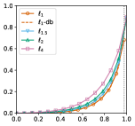
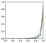
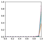
	ATPP	ATPP	ATPP
$\mathrm{AFDP}_{q}-\mathrm{AFDP}_{1}$
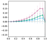
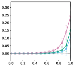
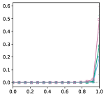
	ATPP	ATPP	ATPP
	$\delta=2$	$\delta=3$	$\delta=4$
AFDP
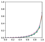
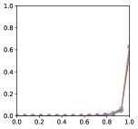
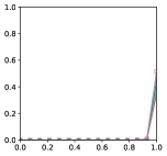
	ATPP	ATPP	ATPP
$\mathrm{AFDP}_{q}-\mathrm{AFDP}_{1}$
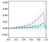
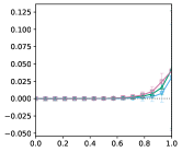
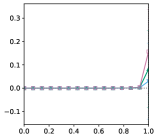
	ATPP	ATPP	ATPP

Figure 5.3: Top row: AFDP-ATPP curve under the setting $\epsilon=0.1,\sigma=0.4,\delta\in\{2,3,4\}$. Second row: Y-axis is the difference of AFDP between the other bridge estimators and LASSO. One standard deviation of the difference is added. Third and fourth rows: the same type of plots as in the first two rows, under the setting $\epsilon=0.3,\sigma=0.4,\delta\in\{2,3,4\}$.

1. $\epsilon=0.1$, $\sigma=0.4$: The results for this setting are shown in Figure 5.3. We vary $\delta\in\{2,3,4\}$. As is clear, LASSO starts to outperform the others even when $\delta=2$. As $\delta$ increases, LASSO remains the best, but all the methods are becoming better and the AFDP-ATPP curves get closer to each other.

2. $\epsilon=0.3$, $\sigma=0.4$: The results can be found in Figure 5.3. Again $\delta\in\{2,3,4\}$. Similar phenomena are observed. Compared to the previous setting, a larger $\epsilon$ leads to a higher SNR and all the methods have improved performances.

3. $\epsilon=0.4$, $\sigma=0.22$: The results are shown in Figure 5.4. We set $\delta\in\{0.7,0.8,1.2\}$. When $\delta$ is 0.7 or 0.8, ridge significantly outperforms the others. As $\delta$ is increased to 1.2, LASSO starts to lead the performances.

	$\delta=0.7$	$\delta=0.8$	$\delta=1.2$
AFDP
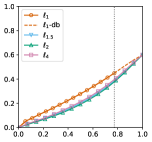
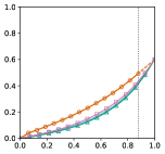
	ATPP	ATPP	ATPP
$\mathrm{AFDP}_{q}-\mathrm{AFDP}_{1}$
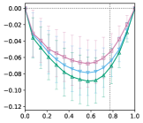
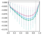
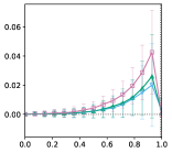
	ATPP	ATPP	ATPP

Figure 5.4: Top row: AFDP-ATPP curve under the setting $\epsilon=0.4,\sigma=0.22,\delta\in\{0.7,0.8,1.2\}$. Second row: Y-axis is the difference of AFDP between the other bridge estimators and LASSO. One standard deviation of the difference is added.

5.5 Nearly black object

In this section, we verify our theoretical results which are presented in Section 3.2.2 for the nearly black object setting. Recall $b_{\epsilon}=\sqrt{\mathbb{E}G^{2}}$ and $\tilde{G}=G/b_{\epsilon}$. We consider the following setting: $\delta=0.8$, $\sigma\in\{3,5\}$, $b_{\epsilon}=4/\sqrt{\epsilon},\tilde{G}=1,\epsilon\in\{0.25,0.0625,0.04\}$. The simulation results are displayed in Figure 5.5. We observe that under both noise levels $\sigma=3,5$, LASSO is suboptimal at sparsity level $\epsilon=0.25$. As $\epsilon$ decreases, LASSO becomes better. When $\epsilon$ is reduced to $0.04$, LASSO outperforms the other bridge estimators by a large margin. Note that in this simulation, the signal strength $b_{\epsilon}$ scales with $\epsilon$ at the rate $\epsilon^{-1/2}$. This is the regime where LASSO is proved to be optimal in Section 3.2.2.

	$\sigma=3$, $\epsilon=0.25$	$\sigma=3$, $\epsilon=0.0625$	$\sigma=3$, $\epsilon=0.04$
AFDP
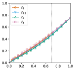
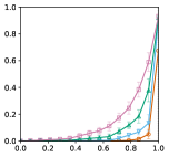
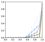
	ATPP	ATPP	ATPP
	$\sigma=5$, $\epsilon=0.25$	$\sigma=5$, $\epsilon=0.0625$	$\sigma=5$, $\epsilon=0.04$
$\mathrm{AFDP}$
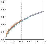
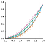
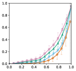
	ATPP	ATPP	ATPP

Figure 5.5: Top row: AFDP-ATPP curve under the setting $b_{\epsilon}=4/\sqrt{\epsilon},\sigma=3,\delta=0.8,\epsilon\in\{0.25,0.0625,0.04\}$. Second row: AFDP-ATPP curve under the setting $b_{\epsilon}=4/\sqrt{\epsilon},\sigma=5,\delta=0.8,\epsilon\in\{0.25,0.0625,0.04\}$. One standard deviation is added.

5.6 LASSO vs. two-stage LASSO

In Theorem 3.2 we proved that two-stage LASSO with its first stage optimally tuned outperforms LASSO on variable selection. We now provide a brief simulation to verify this result. We choose $p_{G}=\delta_{M}$ with $M=8$ and set $\delta=0.8,\epsilon=0.2,\sigma\in\{1,3,5\}$. As shown in Figure 5.6, two-stage LASSO improves over LASSO. When the noise is small ($\sigma=1$), the improvement is the most significant. As the noise level increases, the difference between the two approaches becomes smaller. When the noise is large ($\sigma=5$), both have large errors.

	$\sigma=1$	$\sigma=3$	$\sigma=5$
$\mathrm{AFDP}$
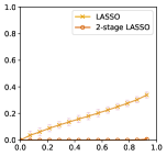
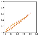
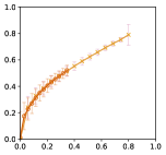
	ATPP	ATPP	ATPP

Figure 5.6: LASSO vs. two-stage LASSO. Here $\delta=0.8$, $\epsilon=0.2$, $M=8,\sigma\in\{1,3,5\}$. The outperformance of two-stage LASSO is the most significant when the noise level is low. When noise gets higher, the gap becomes smaller and smaller.

5.7 General design

In this section, we extend our simulations to general design matrices. Given that our theoretical results in Section 3 are derived under the i.i.d. Gaussian assumption on $X$, the aim of this section is to numerically study the validity scope of our main conclusions when such an assumption does not hold. In particular, we consider the following correlated designs and i.i.d. non-Gaussian designs:

• Correlated design: We consider the model $y=X\Sigma^{\frac{1}{2}}\beta+w$, where $X_{ij}\overset{i.i.d.}{\sim}\mathcal{N}(0,\frac{1}{n})$ and $\Sigma$ is a Toeplitz matrix with $\Sigma_{ij}=\rho^{|i-j|}$. Here $\rho\in(0,1)$ controls the correlation strength.

• i.i.d. non-Gaussian design: We generate $X$ with i.i.d. components $X_{ij}\sim\sqrt{\frac{\nu-2}{n\nu}}t_{\nu}$ where $t_{\nu}$ is the t-distribution with degrees of freedom $\nu$. The scaling $\sqrt{\frac{\nu-2}{n\nu}}$ ensures $\mbox{var}(X_{ij})=\frac{1}{n}$ as in the i.i.d Gaussian case.

Throughout this section, we choose $p=2500,p_{G}=\delta_{M},n=\delta p,w_{i}\overset{i.i.d.}{\sim}N(0,\sigma^{2})$.

Large/small noise

We set $M=8,\delta=0.9$, $\epsilon=0.4$. For correlated design, we vary $\rho\in\{0.1,0.5,0.9\}$ to allow for different levels of correlations among the predictors. Figure 5.7 shows the simulation results. There are a few important observations:

• For a given $\rho\in\{0.1,0.5,0.9\}$, the comparison of bridge estimators under different noise levels is similar to what we observe for i.i.d. Gaussian designs: LASSO performs best in low noise case, and ridge becomes optimal when the noise is large.

• Given the noise level $\sigma=0.8$, as the design correlation $\rho$ varies in $\{0.1,0.5,0.9\}$, it is interesting to observe that, LASSO outperforms the other estimators when the correlation is not high ($\rho=0.1,0.5$), while ridge becomes the optimal one when the correlation is increased to $0.9$. Similar phenomenon happens at the noise level $\sigma=1$. It seems that in terms of variable selection performance comparison of TVS, adding dependency among the predictors is like increasing the noise level in the system. We leave a theoretical analysis of the impact of correlation on our results as an interesting future research.

	$\rho=0.1$, $\sigma=0.8$	$\rho=0.1$, $\sigma=1$	$\rho=0.1$, $\sigma=2$
AFDP
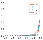
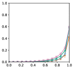
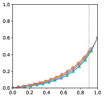
	ATPP	ATPP	ATPP
	$\rho=0.5$, $\sigma=0.8$	$\rho=0.5$, $\sigma=1$	$\rho=0.5$, $\sigma=2$
$\mathrm{AFDP}$
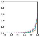
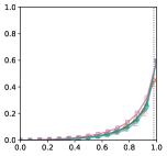
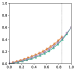
	ATPP	ATPP	ATPP
	$\rho=0.9$, $\sigma=0.3$	$\rho=0.9$, $\sigma=0.8$	$\rho=0.9$, $\sigma=1$
$\mathrm{AFDP}$
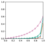
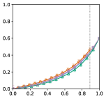
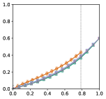
	ATPP	ATPP	ATPP

Figure 5.7: Large/small noise scenario under correlated design.

	$\sigma=0.8$	$\sigma=1$	$\sigma=2$
AFDP
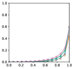
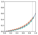
	ATPP	ATPP	ATPP

Figure 5.8: Large/small noise scenario under i.i.d. non-Gaussian design. We set $\delta=0.9,\epsilon=0.4,M=8,\sigma\in\{0.8,1,2\}$. The degrees of freedom of the t-distribution is $\nu=3$.

Regarding i.i.d. non-Gaussian design, we choose the t-distribution $t_{\nu}$ with $\nu=3$. Note that among all the t-distributions $\{t_{\nu},\nu\in\mathbb{N}\}$ with finite variance$,t_{3}$ has the heaviest tail. The results are shown in Figure 5.8. We again observe the comparison predicted by our theory: LASSO outperforms the other bridge estimators when the noise level is low ($\sigma=0.8$), and ridge performs best as the noise level increases to $\sigma=2$.

Nearly black object

For nearly black objects, we consider $\delta=0.8,\sigma=3,b_{\epsilon}=\frac{4}{\sqrt{\epsilon}},\tilde{G}=1,\epsilon\in\{0.25,0.0625,0.04\}$. We construct the design matrix in the following ways:

• Set a correlated Gaussian design with correlation levels $\rho=0.5,0.9$.

• Set an i.i.d. non-Gaussian design with $t_{3}$.

Figures 5.9 and 5.10 contain the results for the correlated design and i.i.d. non-Gaussian design, respectively. We can see that as the model becomes sparser, LASSO starts to outperform other choices of bridge estimator and eventually becomes optimal. This is consistent with the main conclusion we have proved for the i.i.d. Gaussian designs.

	$\rho=0.5$, $\epsilon=0.25$	$\rho=0.5$, $\epsilon=0.0625$	$\rho=0.5$, $\epsilon=0.04$
AFDP
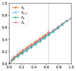
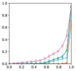
	ATPP	ATPP	ATPP
	$\rho=0.9$, $\epsilon=0.25$	$\rho=0.9$, $\epsilon=0.0625$	$\rho=0.9$, $\epsilon=0.04$
$\mathrm{AFDP}$
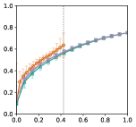
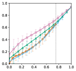
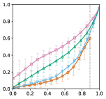
	ATPP	ATPP	ATPP

Figure 5.9: Nearly black object with correlated design. We fix $\delta=0.8$, $\sigma=3$ and $b_{\epsilon}=4/\sqrt{\epsilon},\epsilon\in\{0.25,0.0625,0.04\}$. The correlation $\rho$ is set to $0.5$ and $0.9$ in the two rows.

	$\epsilon=0.25$	$\epsilon=0.0625$	$\epsilon=0.04$
AFDP
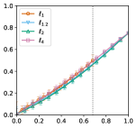
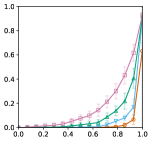
	ATPP	ATPP	ATPP

Figure 5.10: Nearly black object with i.i.d. non-Gaussian design. We fix $\delta=0.8$, $\sigma=3$ and $b_{\epsilon}=4/\sqrt{\epsilon},\epsilon\in\{0.25,0.0625,0.04\}$. The degrees of freedom for the t-distribution design is $\nu=3$.

LASSO vs two-stage LASSO

We compare LASSO and two-stage LASSO under more general designs. As in Section 5.6 for i.i.d. Gaussian design, we set $\delta=0.8$, $\epsilon=0.2$, $M=8$ and $\sigma=1,3,5$. For correlated designs, we pick $\rho=0.5,0.9$. For i.i.d. non-Guassian design, we choose $\nu=3$. As is seen in Figure 5.11, the same phenomenon observed in i.i.d. Gaussian design also occurs under general designs: two-stage LASSO outperforms LASSO by a large margin when the noise is small, and the outperformance becomes marginal in large noise.

	$\rho=0.5$, $\sigma=1$	$\rho=0.5$, $\sigma=3$	$\rho=0.5$, $\sigma=5$
AFDP
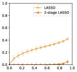
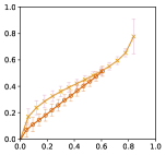
	ATPP	ATPP	ATPP
	$\rho=0.9$, $\sigma=1$	$\rho=0.9$, $\sigma=3$	$\rho=0.9$, $\sigma=5$
$\mathrm{AFDP}$
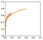
	ATPP	ATPP	ATPP
	$\nu=3$, $\sigma=1$	$\nu=3$, $\sigma=3$	$\nu=3$, $\sigma=5$
$\mathrm{AFDP}$
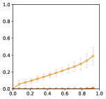
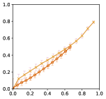
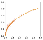
	ATPP	ATPP	ATPP

Figure 5.11: LASSO vs. two-stage LASSO under general designs. Here $\delta=0.8,\epsilon=0.2,M=8,\sigma\in\{1,3,5\}$. The first two rows are for $\rho=0.5,0.9$ in correlated design. The last row is for $\nu=3$ in i.i.d. non-Gaussian design.

6 Discussion

6.1 Nonconvex bridge estimators

In this paper, our discussion has been focused on the bridge estimators with $q\in[1,\infty)$. When $q$ falls in $[0,1)$, the corresponding bridge regression becomes a nonconvex problem. Given that certain nonconvex regularizations have been shown to achieve variable selection consistency under weaker conditions than LASSO [LW⁺17], it is of great interest to analyze the variable selection performance of nonconvex bridge estimators. An early work [HHM⁺08] has showed that bridge estimators for $q\in(0,1)$ enjoy an oracle property in the sense of [FL01] under appropriate conditions. However, the asymptotic regime considered in [HHM⁺08] is fundamentally different from the linear asymptotic in the current paper. A more relevant work is [ZMW⁺17] which studied the estimation property of bridge regression when $q$ belongs to $[0,1]$ under a similar asymptotic framework to ours. Nevertheless, the main focus of [ZMW⁺17] is on the estimators returned by an iterative local algorithm. The analysis of the global minimizer in [ZMW⁺17] relies on the replica method [RGF09] from statistical physics, which has not been fully rigorous yet. To the best of our knowledge, under the linear asymptotic setting, no existing works have provided a fully rigorous analysis of the global solution from nonconvex regularization in linear regression models. We leave this important and challenging problem as a future research.

6.2 Tuning parameter selection for a two-stage variable selection scheme

Two-stage variable selection techniques discussed in this paper have two tuning parameters: the regularization parameter $\lambda$ in the first stage and the threshold $s$ from the second stage. Furthermore, given that TVS using different bridge estimators offer the best performance in different regimes, we may see $q$ as another tuning parameter. How can these parameters be optimally tuned in practice? As proved in Section 3, the TVS with an estimator of smaller AMSE in the first stage provides a better variable selection. Hence, the parameter $\lambda$ can be set by minimizing the estimated risk of the bridge estimator. Similarly, one can estimate the risk for different values of $q$ and choose the one that offers the smallest estimated risk. Section 5.2 has showed how this can be done.

It remains to determine the parameter $s$. As presented in our results, the threshold $s$ controls the trade-off between AFDP and ATPP. By increasing $s$ we decrease the number of false discoveries, but at the same time, we decrease the number of correct discoveries. Therefore, the choice of $s$ depends on the accepted level of false discoveries (or similar quantities). For instance, one can control the false discovery rate by combining the two-stage approach with the knockoff framework [BC⁺15]. Specifically, if we would like to control FDP at a rate of $\rho\in(0,1)$, we can go through the following procedure.

1. Construct the knockoff features $\tilde{X}\in\mathbb{R}^{n\times p}$ as stated in [BC⁺15];

2. Run bridge regression on the joint design $[X,\tilde{X}]$ and obtain the corresponding estimator $\begin{bmatrix}\hat{\beta}\\ \tilde{\beta}\end{bmatrix}$. Let $W_{j}=\max(|\hat{\beta}_{j}|,|\tilde{\beta}_{j}|)\mathrm{sign}(|\hat{\beta}_{j}|-|\tilde{\beta}_{j}|),j=1,2,\ldots,p$. Define the threshold $s$ as $s=\min\Big{\{}t>0:\frac{1+\#\{j:W_{j}\leq-t\}}{\#\{j:W_{j}\geq t\}\vee 1}\leq\rho\Big{\}}$.

3. Select all the predictors with $\{j:W_{j}\geq s\}$.

The above procedure only works for $n\geq p$. We may adapt the new knockoff approach in [CFJL18] when $n<p$.

7 Conclusion

We studied two-stage variable selection schemes for linear models under the high-dimensional asymptotic setting, where the number of observations $n$ grows at the same rate as the number of predictors $p$. Our TVS has a bridge estimator in the first stage and a simple threshold function in the second stage. For such schemes, we proved that for a fixed ATPP, in order to obtain the smallest AFDP one should pick an estimator that minimizes the asymptotic mean square error in the first stage of TVS. This connection between parameter estimation and variable selection further led us to a thorough investigation of the AMSE under different regimes including rare and weak signals, small/large noise, and large sample. Our analyses revealed several interesting phenomena and provided new insights into variable selection. For instance, the variable selection of LASSO can be improved by debiasing and thresholding; a TVS with ridge in its first stage outperforms TVS with other bridge estimators for large values of noise; the optimality of two-stage LASSO among two-stage bridge estimators holds for very sparse signals until the signal strength is below some threshold. We conducted extensive numerical experiments to support our theoretical findings and validate the scope of our main conclusions for general design matrices.

Supplementary material

Appendix A Organization

This supplement contains the proofs of all the main results. Below we mention the organization of this supplement to help the readers.

1. Appendix B includes some preliminaries that will be extensively used in the latter proofs. We also outline the proofs of Theorems 3.3 - 3.8 in Appendix E - I since they share certain similarities.

2. Appendix C proves Lemma 2.2.

3. Appendix D contains the proof of Theorems 3.1, 3.2 and Corollary 3.1.

4. Appendix E proves Theorem 3.3.

5. Appendix F proves Theorem 3.4.

6. Appendix G proves Theorem 3.5.

7. Appendix H proves Theorems 3.6.

8. Appendix I proves Theorem 3.8.

9. Appendix J includes the proof of Theorems 4.1, 4.2, 4.3 and Lemma 4.1.

Appendix B Preliminaries

B.1 Some notations

We will use the following notations throughout this supplementary file:

1. We will use $\partial_{i}f$ to denote the partial derivative of $f(x,y,\ldots)$ with respect to its $i^{\rm th}$ argument. Also for the ease of organizing the proof, we may use $\partial_{y}f$ to be the partial derivative of $f$ with respect to its argument $y$, which is equivalent to $\partial_{2}f$.

2. We will use DCT as a short name for Dominated Convergence Theorem.

3. Recall we have $p_{B}=(1-\epsilon)\delta_{0}+\epsilon p_{G}$. By symmetry, it can be easily verified that $B$ and $G$ appearing in the subsequent proofs can be equivalently replaced by $|B|$ and $|G|$. Hence without loss of generality, we assume $B$ and $G$ are nonnegative random variables.

4. Let $\Phi$ and $\phi$ denote the cumulative distribution function and probability density function of a standard normal random variable respectively. Integration by parts gives us the standard result on the Gaussian tails expansion: for $k\in\mathbb{N}^{+},s>0$

   $$\Phi(-s)=\phi(s)\Bigg{[}\sum_{i=0}^{k-1}\frac{(-1)^{i}(2i-1)!!}{s^{2i+1}}+(-1)^{k}(2k-1)!!\int_{s}^{\infty}\frac{\phi(t)}{t^{2k}}dt\Bigg{]},$$ (B.1)

   where $(2i-1)!!\triangleq 1\times 3\times 5\times\ldots\times(2i-1)$.

5. As $a\rightarrow 0$ (or $a\rightarrow\infty$), $g(a)=O(f(a))$, means that there exists a constant $C$ such that for small enough (or large enough) values of $a$, $g(a)\leq Cf(a)$. Furthermore, $g(a)=o(f(a))$ if and only if $\lim_{a\rightarrow 0}\frac{g(a)}{f(a)}=0$ (or in case of $a\rightarrow\infty$, $\lim_{a\rightarrow\infty}\frac{g(a)}{f(a)}=0$).

6. As $a\rightarrow 0$ (or $a\rightarrow\infty$), $g(a)=\Omega(f(a))$, if and only if $f(a)=O(g(a))$. Similarly, $g(a)=\omega(f(a))$ if and only if $f(a)=o(g(a))$. Finally, $f(a)=\Theta(g(a))$, if and only if $f(a)=O(g(a))$ and $g(a)=O(f(a))$.

B.2 State evolution and properties of the proximal operator

Definition B.1 (pseudo-Lipschitz function).

A function $\psi:\mathbb{R}^{2}\rightarrow\mathbb{R}$ is said to be pseudo-Lipschitz, if $\exists L>0$ s.t., $\forall x,y\in\mathbb{R}^{2}$, $|\psi(x)-\psi(y)|\leq L(1+\|x\|_{2}+\|y\|_{2})\|x-y\|_{2}$.

The following theorem proved by [BM11] and [WMZ⁺18] will be used in our proof.

Theorem B.1.

([BM11], [WMZ⁺18]) For a given $q\in[1,\infty)$, let $\hat{\beta}(q,\lambda)$ be the bridge estimator defined in (1.2). Consider a converging sequence $\{\beta(p),X(p),w(p)\}$. Then, for any pseudo-Lipschitz function $\psi:\mathbb{R}^{2}\rightarrow\mathbb{R}$, almost surely

$$\lim_{p\rightarrow\infty}\frac{1}{p}\sum_{i=1}^{p}\psi\left(\hat{\beta}_{i}(q,\lambda),\beta_{i}(p)\right)=\mathbb{E}\psi\left(\eta_{q}(B+\tau Z;\alpha\tau^{2-q}),B\right),$$

where $B\sim p_{B}$ and $Z\sim N(0,1)$ are two independent random variables; $\alpha$ and $\tau$ are two positive numbers satisfying (2.3) and (2.4).

For each tuning parameter $\lambda>0$, [WMZ⁺18] has proved that the solution pair $(\alpha,\tau)$ to the nonlinear equations (2.3) and (2.4) is unique. We will denote this unique solution pair for the optimal tuning value $\lambda=\lambda_{q}^{*}$ by $(\alpha_{*},\tau_{*})$. Note that we omit the dependency of these two quantities on $q$, since when they appear in this paper, $q$ is clear from the context.

Lemma B.1.

If $(\alpha_{*},\tau_{*})$ are the solutions of (2.3) and (2.4) for $\lambda=\lambda_{q}^{*}$, then $\tau_{*}$ satisfies the following equation:

$$\tau_{*}^{2}= \sigma^{2}+\frac{1}{\delta}\min_{\alpha>0}\mathbb{E}(\eta_{q}(B+\tau_{*}Z;\alpha\tau_{*}^{2-q})-B)^{2},$$

$$\alpha_{*}= \arg\min_{\alpha>0}\mathbb{E}(\eta_{q}(B+\tau_{*}Z;\alpha\tau_{*}^{2-q})-B)^{2}$$ (B.2)

and

$${\rm AMSE}(q,\lambda^{*}_{q})=\mathbb{E}(\eta_{q}(B+\tau_{*}Z;\alpha_{*}\tau_{*}^{2-q})-B)^{2}.$$

This is a simple extension of Lemma 15 in Appendix E of [WMZ⁺18]. Hence we skip the proof. Define

$$R_{q}(\alpha,\tau) \triangleq \mathbb{E}(\eta_{q}(B/\tau+Z;\alpha)-B/\tau)^{2},$$ (B.3)

$$\alpha_{q}(\tau) \triangleq \arg\min_{\alpha\geq 0}R_{q}(\alpha,\tau).$$ (B.4)

For the definition (B.4), if the minimizer is not unique, we choose the smallest one.

Recall the proximal operator:

$$\eta_{q}(u;\chi)=\arg\min_{z}\frac{1}{2}(u-z)^{2}+\chi|z|^{q}.$$

Note that $\eta_{q}(u;\chi)$ does not have an explicit form except for $q=0,1,2$. In the following lemma, we summarize some properties of $\eta_{q}(u;\chi)$. They will be used to prove our theorems.

Lemma B.2.

For any $q\in(1,\infty)$, we have

• $\eta_{q}(u;\chi)=-\eta_{q}(-u;\chi)$.

• $u=\eta_{q}(u;\chi)+\chi q|\eta_{q}(u;\chi)|^{q-1}{\rm sgn}(u)$, where ${\rm sgn}$ denotes the sign of a variable.

• $\eta_{q}(\alpha u;\alpha^{2-q}\chi)=\alpha\eta_{q}(u;\chi),\mbox{~{}~{}for~{}}\alpha>0.$

• $\partial_{1}\eta_{q}(u;\chi)=\frac{1}{1+\chi q(q-1)|\eta_{q}(u;\chi)|^{q-2}}$.

• $\partial_{2}\eta_{q}(u;\chi)=\frac{-q|\eta_{q}(u;\chi)|^{q-1}{\rm sgn}(u)}{1+\chi q(q-1)|\eta_{q}(u;\chi)|^{q-2}}$.

• $0\leq\partial_{1}\eta_{q}(u;\chi)\leq 1$.

• If $1<q<2$, then $\lim_{u\rightarrow 0}\frac{|u|}{|\eta_{q}(u;\chi)|^{q-1}}=\chi q$.

• If $1<q<2$, then $\lim_{u\rightarrow\infty}\frac{|u|}{|\eta_{q}(u;\chi)|}=1$,

Proof.

Please refer to Lemmas 7 and 10 in [WMZ⁺18] for the proof of $q\in(1,2]$. The proof for $q>2$ is the same. Hence we do not repeat it. ∎

B.3 Proof sketch for Theorem 3.3 - 3.8

In Appendix E - I we prove Theorem 3.3 - 3.8. Since the proofs share some similarities, we sketch the proof idea in this section.

The results in Theorem 3.3 - 3.8 characterize the asymptotic expansion of the optimal $\mathrm{AMSE}(q,\lambda_{q}^{*})$ under different scenarios we considered. In Lemma B.1, we connect $\mathrm{AMSE}(q,\lambda_{q}^{*})$ with $(\alpha_{*},\tau_{*})$ through the state evolution equations. Hence in order to prove our theorems, we will characterize the behavior of the solution $(\alpha_{*},\tau_{*})$ of the fixed point equations (2.3) and (2.4) with $\lambda=\lambda_{q}^{*}$ under different scenarios. This can be achieved by making use of (B.1) and its first order condition (notice $\alpha_{*}$ minimize the AMSE).

Depending on different scenarios, (B.1) may be presented in slightly different ways. Specifically for nearly black object, we replace $B$ by $b_{\epsilon}\tilde{B}$ with $p_{\tilde{B}}=(1-\epsilon)\delta_{0}+\epsilon p_{\tilde{G}}$; For large sample scenario, we replace $\sigma^{2}$ by $\frac{\sigma^{2}}{\delta}$.

For $R_{q}(\alpha,\tau)$, the following decomposition holds:

$$R_{q}(\alpha,\tau)=(1-\epsilon)\mathbb{E}\eta_{q}^{2}(Z;\alpha)+\epsilon\mathbb{E}[\eta_{q}(G/\tau+Z;\alpha)-G/\tau]^{2}.$$

Since both terms are positve, either can be used as a lower bound for $R_{q}(\alpha,\tau)$.

For LASSO, the $\ell_{1}$ norm enables a simple form for $\eta_{1}$ and hence for $\eqref{eq:se11}$ and its first order derivative. We present some useful formula below.

$$R_{1}(\alpha,\tau)= \underbrace{(1-\epsilon)\tau^{2}\mathbb{E}\eta_{1}^{2}(Z;\alpha)}_{\triangleq F_{1}}+\underbrace{\epsilon\mathbb{E}[\eta_{1}(b_{\epsilon}\tilde{G}+\tau Z;\alpha\tau)-b_{\epsilon}\tilde{G}-\tau Z]^{2}}_{\triangleq F_{2}}-\underbrace{\epsilon\tau^{2}}_{\triangleq F_{3}}$$

$$+\underbrace{2\epsilon\tau^{2}\mathbb{E}\partial_{1}\eta_{1}(b_{\epsilon}\tilde{G}+\tau Z;\alpha\tau)}_{\triangleq F_{4}}$$ (B.5)

$$= 2(1-\epsilon)[(1+\alpha^{2})\Phi(-\alpha)-\alpha\phi(\alpha)]+\epsilon\mathbb{E}_{G}\bigg{[}(1+\alpha^{2}-\frac{G^{2}}{\tau^{2}})\Phi(\frac{G}{\tau}-\alpha)+$$

$$(1+\alpha^{2}-\frac{G^{2}}{\tau^{2}})\Phi(-\frac{G}{\tau}-\alpha)-(\alpha+\frac{G}{\tau})\phi(\alpha-\frac{G}{\tau})-(\alpha-\frac{G}{\tau})\phi(\alpha+\frac{G}{\tau})+\frac{G^{2}}{\tau^{2}}\bigg{]}$$ (B.6)

Each of the two expansions (B.5) and (B.6) will be handy in certain case. Note that

$$F_{1}=2(1-\epsilon)\tau^{2}\int_{\alpha}^{\infty}(z-\alpha)^{2}\phi(z)dz=2(1-\epsilon)[(1+\alpha^{2})\Phi(-\alpha)-\alpha\phi(\alpha)].$$ (B.7)

We also provide the following expansion for the first order derivative $\partial_{\alpha}R_{1}(\alpha,\tau)$.

$$\frac{\partial R_{1}(\alpha,\tau)}{\partial\alpha}= 2(1-\epsilon)[-\phi(\alpha)+\alpha\Phi(-\alpha)]+\epsilon\mathbb{E}\Big{[}\alpha\Phi(\frac{|G|}{\tau}-\alpha)-\phi(\alpha-\frac{|G|}{\tau})\Big{]}$$

$$+\epsilon\mathbb{E}\Big{[}\alpha\Phi(-\frac{|G|}{\tau}-\alpha)-\phi(\alpha+\frac{|G|}{\tau})\Big{]}$$ (B.8)

Appendix C Proof of Lemma 2.2

Define ${\rm FP}=\sum_{i=1}^{p}\mathbb{I}(\bar{\beta}_{i}(q,\lambda,s)\neq 0,\beta_{i}=0),~{}~{}{\rm TP}=\sum_{i=1}^{p}\mathbb{I}(\bar{\beta}_{i}(q,\lambda,s)\neq 0,\beta_{i}\neq 0)$. First note that according to Theorem B.1, almost surely the empirical distribution of $(\hat{\beta}(q,\lambda),\beta)$ converges weakly to the distribution of $(\eta_{q}(B+\tau Z;\alpha\tau^{2-q}),B)$. We now choose a sequence $t_{m}\rightarrow 0$ as $m\rightarrow 0$ such that $G$ does not have any point mass on that sequence. Then by portmanteau lemma we have almost surely

$$\lim_{p\rightarrow\infty}\frac{1}{p}\sum_{i=1}^{p}\mathbb{I}(\bar{\beta}_{i}(q,\lambda,s)\neq 0,|\beta_{i}|\leq t_{m})=\lim_{p\rightarrow\infty}\frac{1}{p}\sum_{i=1}^{p}\mathbb{I}(|\hat{\beta}_{i}(q,\lambda)|>s,|\beta_{i}|\leq t_{m})$$

$$= \mathbb{P}(|\eta_{q}(B+\tau Z;\alpha\tau^{2-q})|>s,|B|\leq t_{m})$$

$$= (1-\epsilon)\mathbb{P}(|\eta_{q}(\tau Z;\alpha\tau^{2-q})|>s)+\epsilon\mathbb{P}(|\eta_{q}(G+\tau Z;\alpha\tau^{2-q})|>s,|G|\leq t_{m}),$$

which leads to

$$\lim_{m\rightarrow\infty}\lim_{p\rightarrow\infty}\frac{1}{p}\sum_{i=1}^{p}\mathbb{I}(\bar{\beta}_{i}(q,\lambda,s)\neq 0,|\beta_{i}|\leq t_{m})=(1-\epsilon)\mathbb{P}(|\eta_{q}(\tau Z;\alpha\tau^{2-q})|>s).$$

Moreover, it is clear that

$$\frac{1}{p}\big{|}\sum_{i=1}^{p}\mathbb{I}(\bar{\beta}_{i}(q,\lambda,s)\neq 0,|\beta_{i}|\leq t_{m})-{\rm FP}\big{|}\leq\frac{1}{p}\sum_{i=1}^{p}\mathbb{I}(|\hat{\beta}_{i}(q,\lambda)|>s)\cdot\mathbb{I}(0<|\beta_{i}|\leq t_{m})$$

$$\leq\sqrt{\frac{1}{p}\sum_{i=1}^{p}\mathbb{I}(|\hat{\beta}_{i}(q,\lambda)|>s)}\cdot\sqrt{\frac{1}{p}\sum_{i=1}^{p}\mathbb{I}(0<|\beta_{i}|\leq t_{m})}$$

$$\overset{a.s.}{\rightarrow}[\mathbb{P}(|\eta_{q}(B+\tau Z;\alpha\tau^{2-q})|>s)]^{1/2}\cdot\epsilon^{1/2}[\mathbb{P}(0<|G|\leq t_{m})]^{1/2}\mbox{~{}as~{}}p\rightarrow\infty.$$

Hence we obtain almost surely

$$\lim_{m\rightarrow\infty}\lim_{p\rightarrow\infty}\frac{1}{p}\bigg{|}\sum_{i=1}^{p}\mathbb{I}(\bar{\beta}_{i}(q,\lambda,s)\neq 0,|\beta_{i}|\leq t_{m})-{\rm FP}\bigg{|}=0.$$

This combined with (C) implies that as $p\rightarrow\infty$

$$\frac{{\rm FP}}{p}\overset{a.s.}{\rightarrow}(1-\epsilon)\mathbb{P}(|\eta_{q}(\tau Z;\alpha\tau^{2-q})|>s).$$

We can now conclude that

$${\rm AFDP}(q,\lambda,s)=\frac{\lim_{p\rightarrow\infty}{\rm FP}/p}{\lim_{p\rightarrow\infty}\sum_{i=1}^{p}\mathbb{I}(\hat{\beta}_{i}(q,\lambda)>s)/p}\\ =\frac{(1-\epsilon)\mathbb{P}(|\eta_{q}(\tau Z;\alpha\tau^{2-q})|>s)}{\mathbb{P}(|\eta_{q}(B+\tau Z;\alpha\tau^{2-q})|>s)},\quad a.s.$$

The formula of ${\rm AFDP}(q,\lambda,s)$ in Lemma 2.2 can then be obtained by Lemma B.2 part (iii). Regarding ${\rm ATPP}(q,\lambda,s)$ we have

$${\rm ATPP}(q,\lambda,s)= \frac{\lim_{p\rightarrow\infty}\sum_{i=1}^{p}\mathbb{I}(\hat{\beta}_{i}(q,\lambda)>s)/p-\lim_{p\rightarrow\infty}{\rm FP}/p}{\lim_{p\rightarrow\infty}\sum_{i=1}^{p}\mathbb{I}(\beta_{i}\neq 0)/p}$$

$$= \mathbb{P}(|\eta_{q}(G+\tau Z;\alpha\tau^{2-q})|>s),\quad\text{a.s.}$$

Appendix D Proof of Theorems 3.1, 3.2 and Corollary 3.1

We present the proofs of Theorems 3.1, 3.2 and Corollary 3.1 in Sections D.1, D.2 and D.3, respectively.

D.1 Proof of Theorem 3.1

Proof.

According to Lemma 2.2, we know

$${\rm ATPP}(q,\lambda,s)=\mathbb{P}(|\eta_{q}(G+\tau Z;\alpha\tau^{2-q})|>s)$$

where $(\alpha,\tau)$ is the unique solution to (2.3) and (2.4). From Lemma B.2 part (iv), the proximal function $\eta_{q}(u;\chi)=0$ if and only if $u=0$ for $q>1$. Since $G+\tau Z\neq 0~{}a.s.$, we have ${\rm ATPP}(q,\lambda,0)=1$. Moreover, it is clear that ${\rm ATPP}(q,\lambda,+\infty)=0$, and ${\rm ATPP}(q,\lambda,s)$ is a continuous and strictly decreasing function of $s$ over $[0,\infty]$. Hence there exists a unique $s$ for which ${\rm ATPP}(q,\lambda,s)=\zeta\in[0,1]$.

Now consider all possible pairs $(\lambda,s)$ such that ${\rm ATPP}(q,\lambda,s)=\zeta$. Let $(\alpha_{*},\tau_{*},s_{*})$ be the triplet corresponding to the optimal tuning $\lambda_{q}^{*}$ (it minimizes ${\rm AMSE}(q,\lambda)$), and $(\alpha,\tau,s)$ be the one that corresponds to any other $\lambda$. According to Theorem B.1, we know ${\rm AMSE}(q,\lambda)=\delta(\tau^{2}-\sigma^{2})$. So $\tau_{*}<\tau$. By the strict monotonicity and symmetry of $\eta_{q}$ with respect to its first argument (see Lemma B.2 parts (i)(iv)), ${\rm ATPP}(q,\lambda_{q}^{*},s_{*})={\rm ATPP}(q,\lambda,s)$ implies that

$$\mathbb{P}(|G/\tau_{*}+Z|>\eta_{q}^{-1}(s_{*}/\tau_{*};\alpha_{*}))=\mathbb{P}(|G/\tau+Z|>\eta_{q}^{-1}(s/\tau;\alpha)),$$ (D.1)

where $\eta_{q}^{-1}$ is the inverse function of $\eta_{q}$. Now we claim ${\rm AFDP}(q,\lambda_{q}^{*},s_{*})<{\rm AFDP}(q,\lambda,s)$. Otherwise, from the formula of ${\rm AFDP}$ in (2.5), we will have

$$\mathbb{P}(\eta_{q}(|Z|;\alpha_{*})>s_{*}/\tau_{*})\geq\mathbb{P}(\eta_{q}(|Z|;\alpha)>s/\tau),$$

which is equivalent to $\mathbb{P}(|Z|>\eta_{q}^{-1}(s_{*}/\tau_{*};\alpha_{*}))\geq\mathbb{P}(|Z|>\eta_{q}^{-1}(s/\tau;\alpha)).$ This implies $\eta_{q}^{-1}(s_{*}/\tau_{*};\alpha_{*})\leq\eta_{q}^{-1}(s/\tau;\alpha)$. However, combining this result with $\tau_{*}<\tau$ and the fact that $\mathbb{P}(|\mu+Z|>t)$ is an strictly increasing function of $\mu$ over $[0,\infty)$, we must have

$$\small\mathbb{P}\Big{(}\Big{|}\frac{G}{\tau_{*}}+Z\Big{|}>\eta_{q}^{-1}\Big{(}\frac{s_{*}}{\tau_{*}};\alpha_{*}\Big{)}\Big{)}\geq\mathbb{P}\Big{(}\Big{|}\frac{G}{\tau_{*}}+Z\Big{|}>\eta_{q}^{-1}\Big{(}\frac{s}{\tau};\alpha\Big{)}\Big{)}>\mathbb{P}\Big{(}\Big{|}G/\tau+Z\Big{|}>\eta_{q}^{-1}\Big{(}\frac{s}{\tau};\alpha\Big{)}\Big{)}.$$

This is in contradiction with (D.1). The conclusion follows. ∎

D.2 Proof of Theorem 3.2

According to Lemma 2.1,

$${\rm ATPP}(1,\lambda)=\mathbb{P}(|G+\tau Z|>\alpha\tau)=\mathbb{E}[\Phi(G/\tau-\alpha)+\Phi(-G/\tau-\alpha)].$$

It has been shown in [BM12] that, $\alpha$ is an increasing and continuous function of $\lambda$, and $\alpha\rightarrow\infty$ as $\lambda\rightarrow\infty$. Hence, $\text{ATPP}(1,\lambda)$ is continuous in $\lambda$ and $\lim_{\lambda\rightarrow\infty}\text{ATPP}(1,\lambda)=\lim_{\alpha\rightarrow\infty}\mathbb{P}(|G+\tau Z|>\alpha\tau)=0$. Now let $(\alpha_{*},\tau_{*})$ be the solution to (2.3) and (2.4) when $\lambda=\lambda_{1}^{*}$. As we decrease $\lambda$ from $\infty$ to $\lambda_{1}^{*}$, $\text{ATPP}(1,\lambda)$ continuously changes from $0$ to $\text{ATPP}(1,\lambda_{1}^{*})$. Therefore, for any ATPP level $\zeta\in[0,{\rm ATPP}(1,\lambda_{1}^{*})]$, there always exists at least a value of $\lambda\in[\lambda_{1}^{*},\infty]$ such that ${\rm ATPP}(1,\lambda)=\zeta$. Regarding the thresholded LASSO $\bar{\beta}(1,\lambda_{1}^{*},s)$, Lemma 2.2 shows that

$${\rm ATPP}(1,\lambda_{1}^{*},s)=\mathbb{P}(|\eta_{1}(G+\tau_{*}Z;\alpha_{*}\tau_{*})|>s).$$

Note that when $s=0$ the thresholded LASSO is equal to LASSO and thus ${\rm ATPP}(1,\lambda^{*}_{1},0)={\rm ATPP}(1,\lambda_{1}^{*})$. It is also clear that ${\rm ATPP}(1,\lambda_{1}^{*},s)$ is a continuous and strictly decreasing function of $s$ on $[0,\infty]$. As a result, a unique threshold $s_{\zeta}$ exists s.t. ${\rm ATPP}(1,\lambda_{1}^{*},s_{\zeta})$ reaches a given level $\zeta\in[0,{\rm ATPP}(1,\lambda_{1}^{*})]$. We now compare the AFDP of different estimators that have the same ATPP. Suppose $\hat{\beta}(1,\lambda)$ and $\bar{\beta}(1,\lambda_{1}^{*},s)$ reach the same level of ATPP. We have

$$\mathbb{P}(|\eta_{1}(G+\tau Z;\alpha\tau)|>0)=\mathbb{P}(|\eta_{1}(G+\tau_{*}Z;\alpha_{*}\tau_{*})|>s),$$

which is equivalent to

$$\mathbb{P}(|G/\tau+Z|>\alpha)=\mathbb{P}(|G/\tau_{*}+Z|>\alpha_{*}+s/\tau_{*}).$$ (D.2)

Similar to the argument in the proof of Theorem 3.1, we have $\alpha<\alpha_{*}+s/\tau_{*}$, since otherwise the left hand side in (D.2) will be smaller than the right hand side. Hence, we obtain

$$\mathbb{P}(|Z|>\alpha)>\mathbb{P}(|Z|>\alpha_{*}+s/\tau_{*})=\mathbb{P}(|\eta_{1}(Z;\alpha_{*})|>s/\tau_{*}).$$

This implies ${\rm AFDP}(1,\lambda)>{\rm AFDP}(1,\lambda_{1}^{*},s)$ based on Lemmas 2.1 and 2.2. By the same argument, we can show that $\bar{\beta}(1,\lambda_{1}^{*},s)$ also has smaller AFDP than $\bar{\beta}(1,\lambda,s)$ if $\lambda\neq\lambda_{1}^{*}$.

D.3 Proof of Corollary 3.1

This theorem compares the two-stage estimators $\bar{\beta}(q,\lambda_{q}^{*},s)$ for $q\in[1,\infty)$. Consider $q_{1},q_{2}\geq 1$, and ${\rm AMSE}(q_{1},\lambda^{*}_{q_{1}})<{\rm AMSE}(q_{2},\lambda^{*}_{q_{2}})$. Let $(\alpha_{q_{i}*},\tau_{q_{i}*})$ be the solution to (2.3) and (2.4) when $\lambda=\lambda_{q_{i}}^{*}$, for $i=1,2$. Then, according to Theorem B.1, $\tau_{q_{1}*}<\tau_{q_{2}*}$. Suppose ${\rm ATPP}(q_{1},\lambda_{q_{1}},s_{1})={\rm ATPP}(q_{2},\lambda_{q_{2}},s_{2})$, i.e.,

$$\mathbb{P}(\eta_{q_{1}}(G+\tau_{q_{1}*}Z;\alpha_{q_{1}*}\tau_{q_{1}*}^{2-q_{1}})>s_{1})=\mathbb{P}(\eta_{q_{2}}(G+\tau_{q_{2}*}Z;\alpha_{q_{2}*}\tau_{q_{2}*}^{2-q_{2}})>s_{2}).$$

When the ATPP level is 0 or 1, we see $s_{1}$ and $s_{2}$ are either both $\infty$ or 0. The corresponding AFDP will be the same. We now consider the level of ATPP belong to $(0,1)$. Using arguments similar to the ones presented in the proof of Theorem 3.1, we can conclude $\eta_{q_{1}}^{-1}(s_{1}/\tau_{q_{1}*};\alpha_{q_{1}*})>\eta_{q_{2}}^{-1}(s_{2}/\tau_{q_{2}*};\alpha_{q_{2}*})$. This gives us

$$\mathbb{P}(|\eta_{q_{1}}(Z;\alpha_{q_{1}*})|>s_{1}/\tau_{q_{1}*})=\mathbb{P}(|Z|>\eta_{q_{1}}^{-1}(s_{1}/\tau_{q_{1}*};\alpha_{q_{1}*}))$$

$$<\mathbb{P}(|Z|>\eta_{q_{2}}^{-1}(s_{2}/\tau_{q_{2}*};\alpha_{q_{2}*}))=\mathbb{P}(|\eta_{q_{2}}(Z;\alpha_{q_{2}*})|>s_{2}/\tau_{q_{2}*}),$$

implying ${\rm AFDP}(q_{1},\lambda_{q_{1}},s_{1})<{\rm AFDP}(q_{2},\lambda_{q_{2}},s_{2})$.

Appendix E Proof of Theorem 3.3

E.1 Roadmap of the proof

As we have mentioned in Section B.3, we will characterize the behavior of $(\alpha_{*},\tau_{*})$ defined through equation (B.1). Since we are dealing with the nearly black object model, we replace $B$ by $b_{\epsilon}\tilde{B}$ with $p_{\tilde{B}}=(1-\epsilon)\delta_{0}+\epsilon p_{\tilde{B}}$. We first handle $q<2$ in Section E.2 - E.5. Then in Section E.6 we deal with $q\geq 2$. We will prove in Section E.2 that as $\epsilon\rightarrow 0$, $\tau_{*}\rightarrow\sigma$. Furthermore, it is straightforward to see that $\alpha_{*}\rightarrow\infty$ as $\epsilon\rightarrow 0$. Otherwise, if $\alpha_{*}\rightarrow C$, then

$$\varliminf_{\epsilon\rightarrow 0}\mathbb{E}(\eta_{q}(b_{\epsilon}\tilde{B}+\tau_{*}Z;\alpha_{*}\tau_{*}^{2-q})-b_{\epsilon}\tilde{B})^{2}\geq\varliminf_{\epsilon\rightarrow 0}(1-\epsilon)\mathbb{E}\eta_{q}^{2}(\tau_{*}Z;\alpha_{*}\tau_{*}^{2-q})=\mathbb{E}\eta_{q}^{2}(\sigma Z;C\sigma^{2-q})>0.$$

However, in Section E.2 we will prove that $\lim_{\epsilon\rightarrow 0}\mathbb{E}(\eta_{q}(b_{\epsilon}\tilde{B}+\tau_{*}Z;\alpha_{*}\tau_{*}^{2-q})-b_{\epsilon}\tilde{B})^{2}\rightarrow 0$. In order to show the optimal $\mathrm{AMSE}$ vanishes as $\epsilon\rightarrow 0$, we need to characterize the rate at which $\alpha_{*}\rightarrow\infty$. This requires an accurate analysis of $\arg\min_{\alpha}\tilde{R}_{q}(\alpha,\epsilon,\tau_{*})$, where

$$\tilde{R}_{q}(\alpha,\epsilon,\tau)\triangleq\mathbb{E}(\eta_{q}(b_{\epsilon}\tilde{B}+\tau Z;\alpha\tau^{2-q})-b_{\epsilon}\tilde{B}).$$ (E.1)

We note the slight differences between $\tilde{R}_{q}$ and $R_{q}$ in (B.3) and $\mathrm{AMSE}(q,\lambda_{q}^{*})=\tilde{R}(\alpha_{*},\epsilon,\tau_{*})$. The behavior of $\alpha_{*}$ depends on the relation between $b_{\epsilon}$ and $\epsilon$ in the following way:

• Case I - If $b_{\epsilon}=o(\epsilon^{\frac{1-q}{2}})$, then $\lim_{\epsilon\rightarrow 0}\epsilon^{-1}b_{\epsilon}^{-2}\tilde{R}_{q}(\alpha_{*},\epsilon,\tau_{*})=\mathbb{E}|\tilde{G}|^{2}.$ This claim is proved in Section E.3. Note that $\lim_{\alpha\rightarrow\infty}\tilde{R}_{q}(\alpha,\epsilon,\tau)=\epsilon b_{\epsilon}^{2}\mathbb{E}|\tilde{G}|^{2}$ too.

• Case II - If $b_{\epsilon}=\omega(\epsilon^{\frac{1-q}{2}})$, then $\epsilon^{\frac{q-1}{2q}}b_{\epsilon}^{\frac{(q-1)^{2}}{q}}\alpha_{*}=\Theta(1)$. This claim is proved in Section E.4. Furthermore, we will show that

  $$\epsilon^{-\frac{1}{q}}b_{\epsilon}^{-\frac{2(q-1)}{q}}\tilde{R}_{q}(\alpha_{*},\epsilon,\tau_{*})\rightarrow q(q-1)^{\frac{1}{q}-1}\sigma^{\frac{2}{q}}\big{[}\mathbb{E}|Z|^{\frac{2}{q-1}}\big{]}^{\frac{q-1}{q}}\big{[}\mathbb{E}|\tilde{G}|^{2q-2}\big{]}^{\frac{1}{q}}$$

• Case III - If $b_{\epsilon}=\Theta(\epsilon^{\frac{1-q}{2}})$, then still the optimal choice of $\alpha$ satisfies $\epsilon^{\frac{q-1}{2q}}b_{\epsilon}^{\frac{(q-1)^{2}}{q}}\alpha_{*}=\Theta(1)$. This will be proved in Section E.5. After obtaining this result, we will show

  $$\lim_{\epsilon\rightarrow 0}\epsilon^{-\frac{1}{q}}b_{\epsilon}^{-\frac{2(q-1)}{q}}\tilde{R}_{q}(\alpha_{*},\epsilon,\tau_{*})=\min_{C}h(C),$$

  where $h(C)\triangleq(Cq)^{-\frac{2}{q-1}}\sigma^{2}\mathbb{E}|Z|^{\frac{2}{q-1}}+\mathbb{E}\big{(}\eta_{q}(c_{r}G;C\sigma^{2-q})-c_{r}G\big{)}^{2}$, and $c_{r}\triangleq\lim_{\epsilon\rightarrow 0}b_{\epsilon}\epsilon^{\frac{q-1}{2}}$.

E.2 Proof of $\tau_{*}\rightarrow\sigma$ as $\epsilon\rightarrow 0$

We first prove a simple lemma which helps with bounding the optimal $\tau_{*}^{2}$.

Lemma E.1.

For any value of $\epsilon>0$ we have

$$\sigma^{2}\leq\tau_{*}^{2}\leq\sigma^{2}+\frac{\epsilon b_{\epsilon}^{2}}{\delta}\mathbb{E}\tilde{G}^{2}.$$

Proof.

$\tau_{*}>\sigma$ is clear from $\tau_{*}^{2}=\sigma^{2}+\frac{1}{\delta}\min_{\alpha>0}\tilde{R}_{q}(\alpha,\epsilon,\tau_{*})$. Furthermore,

$$\tau_{*}^{2}-\sigma^{2}=\frac{1}{\delta}\min_{\alpha>0}\tilde{R}_{q}(\alpha,\epsilon,\tau_{*})\leq\frac{1}{\delta}\lim_{\alpha\rightarrow\infty}\tilde{R}_{q}(\alpha,\epsilon,\tau_{*})=\frac{\epsilon b_{\epsilon}^{2}}{\delta}\mathbb{E}\tilde{G}^{2}.$$

∎

If $\sqrt{\epsilon}b_{\epsilon}\rightarrow 0$ as $\epsilon\rightarrow 0$, by Lemma E.1, we have $\tau_{*}\rightarrow\sigma$. So next we focus on the case when $\sqrt{\epsilon}b_{\epsilon}\rightarrow c$, where $c\in(0,\infty)$. In order to prove $\tau_{*}\rightarrow\sigma$ under this case, we prove $\tilde{R}_{q}(\alpha,\epsilon,\tau_{*})\rightarrow 0$ for a specific choice of $\alpha$.

Lemma E.2.

If $\sqrt{\epsilon}b_{\epsilon}\rightarrow c$, and $\tilde{\sigma}^{2}\triangleq\sigma^{2}+\frac{\epsilon b_{\epsilon}^{2}}{\delta}\mathbb{E}\tilde{G}^{2}$, then as $\epsilon\rightarrow 0$

$$\sup_{\sigma\leq\tau\leq\tilde{\sigma}}\tilde{R}_{q}\Big{(}\epsilon^{\frac{(2-q)(q-1)}{-2q}},\epsilon,\tau\Big{)}\rightarrow 0.$$

Proof.

Define $\alpha_{0}\triangleq\epsilon^{\frac{(2-q)(q-1)}{-2q}}$. We have

$$\tilde{R}_{q}(\alpha_{0},\epsilon,\tau)=\underbrace{(1-\epsilon)\mathbb{E}\eta_{q}^{2}(\tau Z;\alpha_{0}\tau^{2-q})}_{\triangleq A_{1}(\epsilon)}+\underbrace{\epsilon\mathbb{E}(\eta_{q}(b_{\epsilon}\tilde{G}+\tau Z;\alpha_{0}\tau^{2-q})-b_{\epsilon}\tilde{G})^{2}}_{\triangleq A_{2}(\epsilon)}$$ (E.2)

We first prove that $\varlimsup_{\epsilon\rightarrow 0}\sup_{\sigma\leq\tau\leq\tilde{\sigma}}A_{1}(\epsilon)=0$. Note that

$$\alpha_{0}^{\frac{2}{q-1}}A_{1}(\epsilon)\overset{(a)}{=}(1-\epsilon)\tau^{2}q^{-\frac{2}{q-1}}\mathbb{E}(|Z|-|\eta_{q}(Z;\alpha_{0})|)^{\frac{2}{q-1}}$$ (E.3)

Equality (a) is due to Lemma B.2 (ii) (iii). Hence,

$$\sup_{\sigma\leq\tau\leq\tilde{\sigma}}\alpha_{0}^{\frac{2}{q-1}}A_{1}(\epsilon)\leq(1-\epsilon)\tilde{\sigma}^{2}q^{-\frac{2}{q-1}}\mathbb{E}|Z|^{\frac{2}{q-1}}.$$

Since $\alpha_{0}\rightarrow\infty$ as $\epsilon\rightarrow 0$, this immediately implies that $\lim_{\epsilon\rightarrow 0}\sup_{\sigma\leq\tau\leq\tilde{\sigma}}A_{1}(\epsilon)=0$. Now we discuss $A_{2}(\epsilon)$. We have

$$A_{2}(\epsilon)= \epsilon\mathbb{E}(\eta_{q}(b_{\epsilon}\tilde{G}+\tau Z;\alpha_{0}\tau^{2-q})-b_{\epsilon}\tilde{G}-\tau Z)^{2}+\epsilon\tau^{2}$$

$$+2\epsilon\tau\mathbb{E}(Z(\eta_{q}(b_{\epsilon}\tilde{G}+\tau Z;\alpha_{0}\tau^{2-q})-b_{\epsilon}\tilde{G}-\tau Z))\triangleq\epsilon B_{1}(\epsilon)+\epsilon\tau^{2}+2\epsilon B_{2}(\epsilon).$$ (E.4)

We study $B_{1}(\epsilon)$ and $B_{2}(\epsilon)$ separately.

$$B_{1}(\epsilon)\overset{(a)}{=}q^{2}\alpha_{0}^{2}\tau^{4-2q}\mathbb{E}|\eta_{q}(b_{\epsilon}\tilde{G}+\tau Z;\alpha_{0}\tau^{2-q})|^{2q-2},$$

where Equality (a) is due to Lemma B.2(ii). We note that the choice of $\alpha_{0}$ implies $\epsilon\alpha_{0}^{2}b_{\epsilon}^{2q-2}\rightarrow 0$. Hence, as $\epsilon\rightarrow 0$

$$\epsilon B_{1}(\epsilon)\leq\epsilon\alpha_{0}^{2}q^{2}\tau^{4-2q}\mathbb{E}|b_{\epsilon}\tilde{G}+\tau Z|^{2q-2}\rightarrow 0$$

It is straightforward to see that $\lim_{\epsilon\rightarrow 0}\sup_{\tau\leq\tilde{\sigma}}\epsilon B_{1}(\epsilon)=0$. Now let us discuss $B_{2}(\epsilon)$. By using Stein’s lemma we have

$$B_{2}(\epsilon)=\tau^{2}\mathbb{E}(\partial_{1}\eta_{q}(b_{\epsilon}\tilde{G}+\tau Z;\alpha_{0}\tau^{2-q})-1)\overset{(a)}{=}\tau^{2}\mathbb{E}\bigg{[}\frac{-\alpha_{0}\tau^{2-q}q(q-1)|\eta_{q}(b_{\epsilon}\tilde{G}+\tau Z;\alpha_{0}\tau)|^{q-2}}{1+\alpha_{0}\tau^{2-q}q(q-1)|\eta_{q}(b_{\epsilon}\tilde{G}+\tau Z;\alpha_{0}\tau^{2-q})|^{q-2}}\bigg{]}.$$

Equality (a) is due to Lemma B.2(v). Hence, $|B_{2}(\epsilon)|<\tau^{2}$ and

$$\sup_{\tau\leq\tilde{\sigma}}|\epsilon B_{2}(\epsilon)|\rightarrow 0.$$ (E.5)

Combining (E.2), (E.3), (E.2), and (E.5) completes the proof. ∎

Now Lemma E.1 implies that $\tau_{*}\in[\sigma,\tilde{\sigma}]$. By combining this observation with Lemma E.2, it is straightforward to conclude that

$$\delta(\tau_{*}^{2}-\sigma^{2})=\min_{\alpha>0}\tilde{R}_{q}(\alpha,\epsilon,\tau_{*})\\ \leq\tilde{R}_{q}\Big{(}\epsilon^{\frac{(2-q)(q-1)}{-2q}},\epsilon,\tau_{*}\Big{)}\leq\sup_{\sigma<\tau<\tilde{\sigma}}\tilde{R}_{q}\Big{(}\epsilon^{\frac{(2-q)(q-1)}{-2q}},\epsilon,\tau\Big{)}\rightarrow 0.$$

This finishes our proof of $\tau_{*}\rightarrow\sigma$.

E.3 Case I - $b_{\epsilon}=o(\epsilon^{\frac{1-q}{2}})$

Since Case I is the simplest case, we start with this one. As discussed in Section E.1, $\alpha_{*}\rightarrow\infty$ as $\epsilon\rightarrow 0$. In Lemma E.3 we use this fact to derive a lower bound for $\tilde{R}_{q}(\alpha,\epsilon,\tau)$, then use it to obtain a finer information about $\alpha_{*}$.

Lemma E.3.

If $\alpha\rightarrow\infty$ and $\tau\rightarrow\sigma>0$ as $\epsilon\rightarrow 0$, then

$$\varliminf_{\epsilon\rightarrow 0}\alpha^{\frac{2}{q-1}}\tilde{R}_{q}(\alpha,\epsilon,\tau)\geq\sigma^{2}q^{-\frac{2}{q-1}}\mathbb{E}|Z|^{\frac{2}{q-1}}$$

Proof.

First note that

$$\alpha^{\frac{2}{q-1}}\tilde{R}_{q}(\alpha,\epsilon,\tau)\overset{(a)}{\geq}(1-\epsilon)\alpha^{\frac{2}{q-1}}\tau^{2}\mathbb{E}\eta_{q}^{2}(Z;\alpha)\overset{(b)}{=}(1-\epsilon)\tau^{2}q^{-\frac{2}{q-1}}\mathbb{E}\big{|}|Z|-|\eta_{q}(Z;\alpha)|\big{|}^{\frac{2}{q-1}}.$$

where inequality (a) is due to Lemma B.2(iii) and inequality (b) is due to Lemma B.2(ii). We note that an application of DCT proves that the last term of expectation converges to $\mathbb{E}|Z|^{\frac{2}{q-1}}$ as $\epsilon\rightarrow 0$. We should mention that it is straightforward to prove that for every $u$, $\eta_{q}(u;\alpha)\rightarrow 0$ as $\alpha\rightarrow\infty$. ∎

The rest of the proof goes as follows: we first use Lemma E.3 to prove $b_{\epsilon}\alpha_{*}^{-\frac{1}{2-q}}\rightarrow 0$. This will further help us to characterize the accurate behavior of $\tilde{R}_{q}(\alpha_{*},\epsilon,\tau_{*})$.

Lemma E.4.

We have $\lim_{\alpha\rightarrow\infty}\tilde{R}_{q}(\alpha,\epsilon,\tau_{*})=\epsilon b_{\epsilon}^{2}\mathbb{E}|\tilde{G}|^{2}$.

The proof of this lemma is straightforward and is hence skipped.

Lemma E.5.

If $b_{\epsilon}=o(\epsilon^{\frac{1-q}{2}})$, then $b_{\epsilon}\alpha_{*}^{-\frac{1}{2-q}}\rightarrow 0$ as $\epsilon\rightarrow 0$.

Proof.

We prove by contradiction. Assume the assertion of the lemma is incorrect, i.e. $\frac{\alpha_{*}}{b_{\epsilon}^{2-q}}=O(1)$. Then,

$$\epsilon^{-1}b_{\epsilon}^{-2}\tilde{R}_{q}(\alpha_{*},\epsilon,\tau_{*})=\big{(}\alpha_{*}^{-1}b_{\epsilon}^{2-q}\big{)}^{\frac{2}{q-1}}\big{(}b_{\epsilon}^{\frac{2}{(q-1)}}\epsilon\big{)}^{-1}\alpha_{*}^{\frac{2}{q-1}}\tilde{R}_{q}(\alpha_{*},\epsilon,\tau_{*}).$$

According to Lemma E.3, since $\alpha_{*}\rightarrow\infty$ and $\tau_{*}\rightarrow\sigma$, we have $\alpha_{*}^{\frac{2}{q-1}}\tilde{R}_{q}(\alpha_{*},\epsilon,\tau_{*})=\Omega(1)$. Furthermore our assumption indicates that $\alpha_{*}^{-1}b_{\epsilon}^{2-q}=\Omega(1)$. Finally, due to the condition of the lemma, we have $b_{\epsilon}^{\frac{2}{(q-1)}}\epsilon\rightarrow 0$. Hence, $\epsilon^{-1}b_{\epsilon}^{-2}\tilde{R}_{q}(\alpha_{*},\epsilon,\tau_{*})\rightarrow\infty$. Based on Lemma E.4, $\lim_{\epsilon\rightarrow 0}\tilde{R}_{q}(\alpha,\epsilon,\tau_{*})$ is proportional to $\epsilon b_{\epsilon}^{2}$. This forms a contradiction with the optimality of $\alpha_{*}$ and completes the proof. ∎

In the next theorem we use Lemma E.5 to characterize $R_{q}(\alpha_{*},\epsilon,\tau_{*})$.

Theorem E.1.

If $b_{\epsilon}=o(\epsilon^{\frac{1-q}{2}})$, then $\varliminf_{\epsilon\rightarrow 0}\frac{\tilde{R}_{q}(\alpha_{*},\epsilon,\tau_{*})}{\epsilon b_{\epsilon}^{2}\mathbb{E}|\tilde{G}|^{2}}\geq 1$.

Proof.

It is not hard to see that $\frac{\tilde{R}(\alpha_{*},\epsilon,\tau_{*})}{\epsilon b_{\epsilon}^{2}}\geq\mathbb{E}\Big{[}\eta_{q}\Big{(}\tilde{G}+\frac{\tau_{*}}{b_{\epsilon}}Z;\tau_{*}^{2-q}\frac{\alpha_{*}}{b_{\epsilon}^{2-q}}\Big{)}-\tilde{G}\Big{]}^{2}$. Since $b_{\epsilon}\rightarrow\infty$ and according to Lemma E.5, $\frac{\alpha_{*}}{b_{\epsilon}^{2-q}}\rightarrow\infty$, it is straightforward to apply DCT and obtain that $\mathbb{E}\Big{[}\eta_{q}\Big{(}\tilde{G}+\frac{\tau_{*}}{b_{\epsilon}}Z;\tau_{*}^{2-q}\frac{\alpha_{*}}{b_{\epsilon}^{2-q}}\Big{)}-\tilde{G}\Big{]}^{2}\rightarrow\mathbb{E}|\tilde{G}|^{2}$. The conclusion then follows. ∎

A direct corollary of Lemma E.4 and Theorem E.1 is if $b_{\epsilon}=o(\epsilon^{\frac{1-q}{2}})$, then $\tilde{R}_{q}(\alpha_{*},\epsilon,\tau_{*})\sim\epsilon b_{\epsilon}^{2}\mathbb{E}|\tilde{G}|^{2}$. This completes the first piece of Theorem 3.3.

E.4 Case II - $b_{\epsilon}=\omega(\epsilon^{\frac{1-q}{2}})$

We first characterize the risk for a specific choice of $\alpha$. This offers an upper bound for $\tilde{R}_{q}(\alpha_{*},\epsilon,\tau_{*})$, and will later help us obtain the exact behavior of $\alpha_{*}$.

Lemma E.6.

Suppose that $b_{\epsilon}=\omega(\epsilon^{\frac{1-q}{2}})$. If $\alpha=C\epsilon^{\frac{1-q}{2q}}b_{\epsilon}^{-\frac{(q-1)^{2}}{q}}$, then,

$$\lim_{\epsilon\rightarrow 0}\epsilon^{-\frac{1}{q}}b_{\epsilon}^{-\frac{2(q-1)}{q}}\tilde{R}(\alpha,\epsilon,\tau_{*})=C^{\frac{-2}{q-1}}q^{-\frac{2}{q-1}}\sigma^{2}\mathbb{E}|Z|^{\frac{2}{q-1}}+C^{2}q^{2}\sigma^{4-2q)}\mathbb{E}|\tilde{G}|^{2(q-1)}.$$

Proof.

We again start our argument with the same decomposition as in (E.2). Note that as $\epsilon\rightarrow 0$, $\alpha\rightarrow\infty$, and as discussed in Section E.2, $\tau_{*}\rightarrow\sigma$. We further have

$$\epsilon^{-\frac{1}{q}}b_{\epsilon}^{\frac{-2(q-1)}{q}}A_{1}(\epsilon)=(1-\epsilon)\epsilon^{-\frac{1}{q}}b_{\epsilon}^{\frac{-2(q-1)}{q}}\tau_{*}^{2}\;\mathbb{E}\eta_{q}^{2}(Z;\alpha)$$ (E.6)

$$\overset{(a)}{=} (1-\epsilon)q^{-\frac{2}{q-1}}\Big{(}\alpha\epsilon^{\frac{q-1}{2q}}b_{\epsilon}^{\frac{(q-1)^{2}}{q}}\Big{)}^{-\frac{2}{q-1}}\tau_{*}^{2}\;\mathbb{E}\big{|}|Z|-|\eta_{q}(Z;\alpha)|\big{|}^{\frac{2}{q-1}}\rightarrow q^{-\frac{2}{q-1}}C^{-\frac{2}{q-1}}\sigma^{2}\mathbb{E}|Z|^{\frac{2}{q-1}}.$$

Equality (a) is due to Lemma B.2(ii), and the last step is a result of DCT. We should also emphasize that since $\alpha\rightarrow\infty$, $|\eta_{q}(Z;\alpha)|\rightarrow 0$. Furthermore, similar to the steps in the proof of Lemma (E.2), we can obtain

$$A_{2}(\epsilon)=\;\epsilon\alpha^{2}\tau_{*}^{4-2q}q^{2}\mathbb{E}\big{|}\eta_{q}(b_{\epsilon}\tilde{G}+\tau_{*}Z;\alpha\tau_{*}^{2-q})\big{|}^{2q-2}+\epsilon\tau_{*}^{2}+2\epsilon\tau_{*}^{2}\mathbb{E}[\partial_{1}\eta_{q}(b_{\epsilon}\tilde{G}+\tau_{*}Z;\alpha\tau_{*}^{2-q})-1].$$ (E.7)

First we have that

$$\epsilon^{-\frac{1}{q}}b_{\epsilon}^{\frac{-2(q-1)}{q}}\epsilon\alpha^{2}\tau_{*}^{4-2q}q^{2}\mathbb{E}\big{|}\eta_{q}(b_{\epsilon}\tilde{G}+\tau_{*}Z;\alpha\tau_{*}^{2-q})\big{|}^{2q-2}$$

$$= \alpha^{2}\epsilon^{\frac{q-1}{q}}b_{\epsilon}^{\frac{2(q-1)^{2}}{q}}\tau_{*}^{4-2q}q^{2}\mathbb{E}\bigg{[}\frac{|\eta_{q}(b_{\epsilon}\alpha^{-\frac{1}{2-q}}\tilde{G}+\alpha^{-\frac{1}{2-q}}\tau_{*}Z;\tau_{*}^{2-q})|}{|b_{\epsilon}\alpha^{-\frac{1}{2-q}}\tilde{G}+\alpha^{-\frac{1}{2-q}}\tau_{*}Z|}|\tilde{G}+b_{\epsilon}^{-1}\tau_{*}Z|\bigg{]}^{2q-2}$$ (E.8)

We note our condition on the growth of $\alpha$ and the following relation:

$$b_{\epsilon}\alpha^{-\frac{1}{2-q}}=C^{-\frac{1}{2-q}}\big{[}\epsilon^{\frac{q-1}{2}}b_{\epsilon}\big{]}^{\frac{1}{q(2-q)}}\rightarrow\infty,\quad\epsilon^{-\frac{1}{q}}b_{\epsilon}^{\frac{-2(q-1)}{q}}\epsilon=\big{[}\epsilon b_{\epsilon}^{-2}\big{]}^{\frac{q-1}{q}}\rightarrow 0$$

The first relation above implies that

$$\lim_{\epsilon\rightarrow 0}\epsilon^{-\frac{1}{q}}b_{\epsilon}^{\frac{-2(q-1)}{q}}\epsilon\alpha^{2}\tau_{*}^{4-2q}q^{2}\mathbb{E}\big{|}\eta_{q}(b_{\epsilon}\tilde{G}+\tau_{*}Z;\alpha\tau_{*}^{2-q})\big{|}^{2q-2}=C^{2}\sigma^{4-2q}q^{2}\mathbb{E}|\tilde{G}|^{2q-2}$$ (E.9)

Since $\big{|}\partial_{1}\eta_{q}(b_{\epsilon}\tilde{G}+\tau_{*}Z;\alpha\tau_{*}^{2-q})-1\big{|}\leq 1$, we are able to conclude that

$$\epsilon^{-\frac{1}{q}}b_{\epsilon}^{\frac{-2(q-1)}{q}}A_{2}(\epsilon)\rightarrow C^{2}\sigma^{4-2q}q^{2}\mathbb{E}|\tilde{G}|^{2q-2}$$ (E.10)

where the last step is a simple application of DCT (According to Lemma B.2(ii) $\frac{|\eta_{q}(u;\chi)|}{|u|}\leq 1$ for every $u$ and $\chi$), combined with the fact that ${b_{\epsilon}}\rightarrow\infty$ and $\tau_{*}\rightarrow\sigma$ as $\epsilon\rightarrow 0$. Combining (E.2), (E.6), (E.7), and (E.10) finishes the proof. ∎

So far, we know that $\alpha_{*}\rightarrow\infty$. Our next theorem provides more accurate information about $\alpha_{*}$.

Theorem E.2.

If $b_{\epsilon}=\omega(\epsilon^{\frac{1-q}{2}})$, then $b_{\epsilon}\alpha_{*}^{-\frac{1}{2-q}}\rightarrow\infty$.

Proof.

Suppose this is not correct, then $b_{\epsilon}\alpha_{*}^{-\frac{1}{2-q}}=O(1)$. According to (E.7) and (E.2) we have

$$\tilde{R}_{q}(\alpha_{*},\epsilon,\tau_{*})\geq \;\epsilon\mathbb{E}\big{(}\eta_{q}(b_{\epsilon}\tilde{G}+\tau_{*}Z;\alpha_{*}\tau_{*}^{2-q})-b_{\epsilon}\tilde{G}\big{)}^{2}$$

$$\overset{(a)}{=} \;\epsilon b_{\epsilon}^{2}\mathbb{E}\big{(}\eta_{q}(\tilde{G}+b_{\epsilon}^{-1}\tau_{*}Z;b_{\epsilon}^{q-2}\alpha_{*}\tau_{*}^{2-q})-\tilde{G}\big{)}^{2},$$ (E.11)

where the last equality is due to Lemma B.2(iii). Note that

$$\frac{\tilde{R}_{q}(\alpha_{*},\epsilon,\tau_{*})}{\tilde{R}_{q}(C\epsilon^{\frac{1-q}{2q}}b_{\epsilon}^{-\frac{(q-1)^{2}}{q}},\epsilon,\tau_{*})}=\frac{\epsilon^{-1}b_{\epsilon}^{-2}\tilde{R}_{q}(\alpha_{*},\epsilon,\tau_{*})}{\epsilon^{-\frac{1}{q}}b_{\epsilon}^{\frac{2(1-q)}{q}}\tilde{R}_{q}(C\epsilon^{\frac{1-q}{2q}}b_{\epsilon}^{-\frac{(q-1)^{2}}{q}},\epsilon,\tau_{*})}\times(\epsilon^{q-1}b_{\epsilon}^{2})^{\frac{1}{q}}.$$

According to Lemma E.6, $\epsilon^{-\frac{1}{q}}b_{\epsilon}^{\frac{2(1-q)}{q}}\tilde{R}_{q}(C\epsilon^{\frac{1-q}{2q}}b_{\epsilon}^{-\frac{(q-1)^{2}}{q}},\epsilon,\tau_{*})=\Theta(1)$. By using the DCT in (E.4) (combined with the assumption that $b_{\epsilon}\alpha_{*}^{-\frac{1}{2-q}}=O(1)$), it is straightforward to confirm that $\epsilon^{-1}b_{\epsilon}^{-2}\tilde{R}_{q}(\alpha_{*},\epsilon,\tau_{*})=\Omega(1)$. Since, $(\epsilon^{q-1}b_{\epsilon}^{2})^{\frac{1}{q}}\rightarrow\infty$, we conclude that

$$\varliminf_{\epsilon\rightarrow 0}\frac{\tilde{R}_{q}(\alpha_{*},\epsilon,\tau_{*})}{\tilde{R}_{q}(C\sqrt{\epsilon}^{\frac{1-q}{q}}b_{\epsilon}^{-\frac{(q-1)^{2}}{q}},\epsilon,\tau_{*})}=\infty.$$

This is contradicted with the optimality of $\alpha_{*}$. Hence, $b_{\epsilon}\alpha_{*}^{-\frac{1}{2-q}}\rightarrow\infty$. ∎

Finally, we are ready to prove the main claim of this section.

Theorem E.3.

Suppose that $b_{\epsilon}=\omega(\epsilon^{\frac{1-q}{2}})$. Then, $\epsilon^{\frac{q-1}{2q}}b_{\epsilon}^{\frac{(q-1)^{2}}{q}}\alpha_{*}\rightarrow C_{*}$, where $C_{*}=\bigg{[}\frac{\sigma^{2q-2}\mathbb{E}|Z|^{\frac{2}{q-1}}}{(q-1)q^{\frac{2q}{q-1}}\mathbb{E}|\tilde{G}|^{2q-2}}\bigg{]}^{\frac{q-1}{2q}}$. Furthermore,

$$\epsilon^{-\frac{1}{q}}b_{\epsilon}^{-\frac{2(q-1)}{q}}\tilde{R}_{q}(\alpha_{*},\epsilon,\tau_{*})\rightarrow(C_{*}q)^{\frac{-2}{q-1}}\sigma^{2}\mathbb{E}|Z|^{\frac{2}{q-1}}+(C_{*}q)^{2}\sigma^{4-2q}\mathbb{E}|\tilde{G}|^{2(q-1)}.$$ (E.12)

Proof.

We know that $\frac{\partial\tilde{R}_{q}(\alpha_{*},\epsilon,\tau_{*})}{\partial\alpha}=0$. Hence,

$$0= (1-\epsilon)\tau_{*}^{2}\mathbb{E}[\eta_{q}(Z;\alpha_{*})\partial_{2}\eta_{q}(Z;\alpha_{*})]$$

$$+\epsilon\tau_{*}^{2-q}\mathbb{E}\big{[}(\eta_{q}(b_{\epsilon}\tilde{G}+\tau_{*}Z;\alpha_{*}\tau_{*}^{2-q})-b_{\epsilon}\tilde{G})\partial_{2}\eta_{q}(b_{\epsilon}\tilde{G}+\tau_{*}Z;\alpha_{*}\tau_{*}^{2-q})\big{]}$$

$$\overset{(a)}{=} (1-\epsilon)\tau_{*}^{2}\mathbb{E}\bigg{[}\frac{-q|\eta_{q}(Z;\alpha_{*})|^{q}}{1+\alpha_{*}q(q-1)|\eta_{q}(Z;\alpha_{*})|^{q-2}}\bigg{]}+\epsilon\tau_{*}^{3-q}\mathbb{E}\big{[}Z\partial_{2}\eta_{q}(b_{\epsilon}\tilde{G}+\tau_{*}Z;\alpha_{*}\tau_{*}^{2-q})\big{]}$$

$$+\epsilon\alpha_{*}\tau_{*}^{4-2q}q^{2}\mathbb{E}\bigg{[}\frac{|\eta_{q}(b_{\epsilon}\tilde{G}+\tau_{*}Z;\alpha_{*}\tau_{*}^{2-q})|^{2q-2}}{1+\alpha_{*}\tau_{*}^{2-q}q(q-1)|\eta_{q}(b_{\epsilon}\tilde{G}+\tau_{*}Z;\alpha_{*}\tau_{*}^{2-q})|^{q-2}}\bigg{]}$$

$$\triangleq -(1-\epsilon)q\tau_{*}^{2}H_{1}+\epsilon\tau_{*}^{3-q}H_{2}+\epsilon\alpha_{*}\tau_{*}^{4-2q}q^{2}H_{3}.$$ (E.13)

To obtain (a) we have used Lemma B.2 parts (ii) and (v). We now study each term separately. We should mention at this point that the rest of our analyses relies heavily on Theorem E.2. By using Lemma B.2(iii) we have

$$H_{1}= \mathbb{E}\bigg{[}\frac{|\eta_{q}(Z;\alpha_{*})|^{q}}{1+\alpha_{*}q(q-1)|\eta_{q}(Z;\alpha_{*})|^{q-2}}\bigg{]}$$

$$= \alpha_{*}^{-1}\mathbb{E}\Bigg{[}\bigg{|}\frac{|Z|-|\eta_{q}(Z;\alpha_{*})|}{q\alpha_{*}}\bigg{|}^{\frac{2}{q-1}}\frac{|\eta_{q}(\alpha_{*}^{-\frac{1}{2-q}}Z;1)|^{q-2}}{1+q(q-1)|\eta_{q}(\alpha_{*}^{-\frac{1}{2-q}}Z;1)|^{q-2}}\Bigg{]}.$$ (E.14)

Since $|\eta_{q}(\alpha_{*}^{-\frac{1}{2-q}}Z;1)|\rightarrow 0$, we have

$$\frac{|\eta_{q}(\alpha_{*}^{-\frac{1}{2-q}}Z;1)|^{q-2}}{1+q(q-1)|\eta_{q}(\alpha_{*}^{-\frac{1}{2-q}}Z;1)|^{q-2}}\rightarrow\frac{1}{q(q-1)}.$$ (E.15)

By combining (E.4) and (E.15) we have

$$\alpha_{*}^{\frac{q+1}{q-1}}H_{1}\rightarrow(q-1)^{-1}q^{-\frac{q+1}{q-1}}\mathbb{E}|Z|^{\frac{2}{q-1}}.$$ (E.16)

Now we focus on $H_{3}$. Define $D\triangleq 1+q(q-1)\tau_{*}^{2-q}|\eta_{q}(\frac{b_{\epsilon}\tilde{G}}{\alpha_{*}^{\frac{1}{2-q}}}+\frac{\tau_{*}Z}{\alpha_{*}^{\frac{1}{2-q}}};\tau_{*}^{2-q})|^{q-2}$. Then,

$$H_{3}= \mathbb{E}\bigg{[}\frac{|\eta_{q}(b_{\epsilon}\tilde{G}+\tau_{*}Z;\alpha_{*}\tau_{*}^{2-q})|^{2q-2}}{1+\alpha_{*}\tau_{*}^{2-q}q(q-1)|\eta_{q}(b_{\epsilon}\tilde{G}+\tau_{*}Z;\alpha_{*}\tau_{*}^{2-q})|^{q-2}}\bigg{]}$$

$$= \mathbb{E}\bigg{[}\frac{b_{\epsilon}^{2q-2}|\eta_{q}(\tilde{G}+b_{\epsilon}^{-1}\tau_{*}Z;\alpha_{*}b_{\epsilon}^{q-2}\tau_{*}^{2-q})|^{2q-2}}{1+\alpha_{*}b_{\epsilon}^{q-2}\tau_{*}^{2-q}q(q-1)|\eta_{q}(\tilde{G}+b_{\epsilon}^{-1}\tau_{*}Z;\alpha_{*}b_{\epsilon}^{q-2}\tau_{*}^{2-q})|^{q-2}}\bigg{]}.$$

According to Theorem E.2, $\alpha_{*}b_{\epsilon}^{q-2}\rightarrow 0$. This drives the term $\alpha_{*}\tau_{*}^{2-q}q(q-1)|\eta_{q}(b_{\epsilon}\tilde{G}+\tau_{*}Z;\alpha_{*}\tau_{*}^{2-q})|^{q-2}\rightarrow 0$ in the denominator. It is then straightforward to use DCT and show that

$$\lim_{\epsilon\rightarrow 0}b_{\epsilon}^{2-2q}H_{3}=\mathbb{E}|\tilde{G}|^{2q-2}.$$ (E.17)

Finally, we discuss $H_{2}$. By using Stein’s lemma and after some algebraic calculations we have

$$H_{2}= -q\mathbb{E}\bigg{[}Z\frac{|\eta_{q}(b_{\epsilon}\tilde{G}+\tau_{*}Z;\alpha_{*}\tau_{*}^{2-q})|^{q-1}\mathrm{sign}(b_{\epsilon}\tilde{G}+\tau_{*}Z;\alpha_{*}\tau_{*}^{2-q})}{1+\alpha_{*}\tau_{*}^{2-q}q(q-1)|\eta_{q}(b_{\epsilon}\tilde{G}+\tau_{*}Z)|^{q-2}}\bigg{]}$$

$$= -q(q-1)\tau_{*}\mathbb{E}\bigg{[}\frac{|\eta_{q}(b_{\epsilon}\tilde{G}+\tau_{*}Z;\alpha_{*}\tau_{*}^{2-q})|^{q-2}}{(1+\alpha_{*}\tau_{*}^{2-q}q(q-1)|\eta_{q}(b_{\epsilon}\tilde{G}+\tau_{*}Z;\alpha_{*}\tau_{*}^{2-q})|^{q-2})^{3}}\bigg{]}$$

$$-q^{2}(q-1)\alpha_{*}\tau_{*}^{3-q}\mathbb{E}\bigg{[}\frac{|\eta_{q}(b_{\epsilon}\tilde{G}+\tau_{*}Z;\alpha_{*}\tau_{*}^{2-q})|^{2q-4}}{(1+\alpha_{*}\tau_{*}^{2-q}q(q-1)|\eta_{q}(b_{\epsilon}\tilde{G}+\tau_{*}Z;\alpha_{*}\tau_{*}^{2-q})|^{q-2})^{3}}\bigg{]}$$

$$\triangleq -q(q-1)\tau_{*}H_{4}-q^{2}(q-1)\alpha_{*}\tau_{*}^{3-q}H_{5}.$$

Now we bound $H_{4}$ and $H_{5}$. Due to exactly the same reason when we analyzing $H_{3}$, the denominator of $H_{4}$ and $H_{5}$ converges to 1. According to Lemma B.2(iii), we have

$$b_{\epsilon}^{2-q}H_{4}=\mathbb{E}\bigg{[}\frac{|\eta_{q}(\tilde{G}+b_{\epsilon}^{-1}\tau_{*}Z;\alpha_{*}b_{\epsilon}^{q-2}\tau_{*}^{2-q})|^{q-2}}{(1+\alpha_{*}\tau_{*}^{2-q}q(q-1)|\eta_{q}(b_{\epsilon}\tilde{G}+\tau_{*}Z;\alpha_{*}\tau_{*}^{2-q})|^{q-2})^{3}}\bigg{]}\rightarrow\mathbb{E}|\tilde{G}|^{q-2}$$ (E.18)

Similarly for $H_{5}$ we have that

$$b_{\epsilon}^{4-2q}H_{5}=\mathbb{E}\bigg{[}\frac{|\eta_{q}(\tilde{G}+b_{\epsilon}^{-1}\tau_{*}Z;\alpha_{*}b_{\epsilon}^{q-2}\tau_{*}^{2-q})|^{2q-4}}{(1+\alpha_{*}\tau_{*}^{2-q}q(q-1)|\eta_{q}(b_{\epsilon}\tilde{G}+\tau_{*}Z;\alpha_{*}\tau_{*}^{2-q})|^{q-2})^{3}}\bigg{]}\rightarrow\mathbb{E}|\tilde{G}|^{2q-4}$$ (E.19)

From (E.4) and with some algebra we have

$$1= \lim_{\epsilon\rightarrow 0}\frac{\epsilon\tau_{*}^{3-q}H_{2}+\epsilon\alpha_{*}\tau_{*}^{4-2q}q^{2}H_{3}}{(1-\epsilon)q\tau_{*}^{2}H_{1}}=\lim_{\epsilon\rightarrow 0}\frac{\tau_{*}^{3-q}\alpha_{*}^{-1}b_{\epsilon}^{2-2q}H_{2}+\tau_{*}^{4-2q}q^{2}b_{\epsilon}^{2-2q}H_{3}}{(1-\epsilon)q\tau_{*}^{2}\alpha_{*}^{\frac{q+1}{q-1}}H_{1}}\epsilon\alpha_{*}^{\frac{2q}{q-1}}b_{\epsilon}^{2q-2}$$

$$= \frac{(q-1)q^{\frac{2q}{q-1}}\mathbb{E}|\tilde{G}|^{2q-2}}{\sigma^{2q-2}\mathbb{E}|Z|^{\frac{2}{q-1}}}\lim_{\epsilon\rightarrow 0}\epsilon\alpha_{*}^{\frac{2q}{q-1}}b_{\epsilon}^{2q-2}$$

where in the last step, we use the fact that $\alpha^{-1}b_{\epsilon}^{2-2q}H_{2}\rightarrow 0$ which is an implication of (E.18) and (E.19). We also used (E.16) and (E.17) to simplify the part involving $H_{1}$ and $H_{3}$. Overall, these give us that

$$\lim_{\epsilon\rightarrow 0}\epsilon\alpha_{*}^{\frac{2q}{q-1}}b_{\epsilon}^{2q-2}=\frac{\sigma^{2q-2}\mathbb{E}|Z|^{\frac{2}{q-1}}}{(q-1)q^{\frac{2q}{q-1}}\mathbb{E}|\tilde{G}|^{2q-2}}=C_{*}^{\frac{2q}{q-1}}$$ (E.20)

This proves the first claim of our theorem. The behavior of $\tilde{R}(\alpha_{*},\epsilon,\tau_{*})$ now follows once we combine (E.20) with Lemma E.6. In order to obtain the final form presented in Theorem 3.3, we need to substitute $C_{*}$ into (E.12) and simplify the expression. ∎

E.5 Case III - $\frac{b_{\epsilon}}{\sqrt{\epsilon}^{1-q}}\rightarrow c_{r}$ for $c_{r}\in(0,\infty)$

Since the proof is very similar to the one we presented in the last section, we only present the sketch of the proof, and do not discuss the details. We only emphasize on the major differences. First note that similar to what we had before

$$\tilde{R}_{q}(\alpha,\epsilon,\tau_{*})=(1-\epsilon)\tau_{*}^{2}\mathbb{E}\eta_{q}^{2}(Z;\alpha)+\epsilon\mathbb{E}\big{(}\eta_{q}(b_{\epsilon}\tilde{G}+\tau_{*}Z;\alpha\tau_{*}^{2-q})-b_{\epsilon}\tilde{G}\big{)}^{2}.$$

We can prove the following claims:

1. It is straightforward to prove that

   $$\lim_{\alpha\rightarrow\infty}\tilde{R}_{q}(\alpha,\epsilon,\tau_{*})=\epsilon b_{\epsilon}^{2}\mathbb{E}(\tilde{G})^{2}.$$ (E.21)

2. We claim that $\alpha_{*}^{-\frac{1}{2-q}}b_{\epsilon}=O(1)$. We then have

   $$\varliminf_{\epsilon\rightarrow 0}\alpha_{*}^{\frac{2}{q-1}}\tilde{R}_{q}(\alpha_{*},\epsilon,\tau_{*})\geq\sigma^{2}\varliminf_{\epsilon\rightarrow 0}\alpha_{*}^{\frac{2}{q-1}}\mathbb{E}\eta_{q}^{2}(Z;\alpha_{*})\overset{(a)}{=}\Theta(1).$$ (E.22)

   The reasoning for (a) is similar to what we did in (E.6). We connect (E.21) and (E.22) through the optimality of $\alpha_{*}$ to conclude that

   $$\epsilon b_{\epsilon}^{2}\alpha_{*}^{\frac{2}{q-1}}\geq\Theta(1)$$

   Our claim then follows by substituting the relation $\epsilon\sim b_{\epsilon}^{-\frac{2}{q-1}}$ into the above equation.

3. Given the previous case two scenarios can happen, each of which is discussed below:

   • Case I: $\alpha_{*}^{-\frac{1}{2-q}}b_{\epsilon}\rightarrow 0$. Note that in this case, we have

     $$\varliminf_{\epsilon\rightarrow 0}\frac{\tilde{R}_{q}(\alpha_{*},\epsilon,\tau_{*})}{\epsilon b_{\epsilon}^{2}\mathbb{E}|\tilde{G}|^{2}}\geq\varliminf_{\epsilon\rightarrow 0}\frac{\mathbb{E}\big{(}\eta_{q}(\tilde{G}+b_{\epsilon}^{-1}\tau_{*}Z;\alpha_{*}b_{\epsilon}^{q-2}\tau_{*}^{2-q})-\tilde{G}\big{)}^{2}}{\mathbb{E}|\tilde{G}|^{2}}=1,$$

     where the last step is a result of DCT and the assumption that $\alpha_{*}^{-\frac{1}{2-q}}b_{\epsilon}\rightarrow 0$. Note that the lower bound is achievable by $\alpha=\infty$.

   • Case II: $\alpha_{*}^{-\frac{1}{2-q}}b_{\epsilon}=\Theta(1)$. Under this assumption, we have $\alpha_{*}\epsilon^{\frac{(q-1)(2-q)}{2}}\rightarrow C$, where $C>0$ is fixed. We will specify the optimal choice of $C$ later. Furthermore,

     $$b_{\epsilon}\alpha_{*}^{-\frac{1}{2-q}}\rightarrow c_{r}C^{-\frac{1}{2-q}}.$$

     We remind the reader that $c_{r}\triangleq\lim_{\epsilon\rightarrow 0}\frac{b_{\epsilon}}{\sqrt{\epsilon}^{1-q}}\in(0,\infty)$. Similar to the proof of Lemma E.3 we have

     $$\alpha_{*}^{\frac{2}{q-1}}\mathbb{E}\eta_{q}^{2}(Z;\alpha_{*})\rightarrow q^{-\frac{2}{q-1}}\mathbb{E}|Z|^{\frac{2}{q-1}}.$$ (E.23)

     Also, with DCT we can show that, as $\epsilon\rightarrow 0$

     $$\small{\alpha_{*}^{-\frac{2}{2-q}}\mathbb{E}\big{(}\eta_{q}(b_{\epsilon}\tilde{G}+\tau_{*}Z;\alpha_{*}\tau_{*}^{2-q})-b_{\epsilon}\tilde{G}\big{)}^{2}\rightarrow\mathbb{E}\big{(}\eta_{q}(c_{r}C^{-\frac{1}{2-q}}G;\sigma^{2-q})-c_{r}C^{-\frac{1}{2-q}}G\big{)}^{2}.}$$ (E.24)

     Now we can characterize the risk accurately as

     $$\lim_{\epsilon\rightarrow 0}\epsilon^{q-2}\tilde{R}_{q}(\alpha_{*},\epsilon,\tau_{*})=\lim_{\epsilon\rightarrow 0}\epsilon^{q-2}\alpha_{*}^{-\frac{2}{q-1}}\tau_{*}^{2}\alpha_{*}^{\frac{2}{q-1}}\mathbb{E}\eta_{q}^{2}(Z;\alpha_{*})$$

     $$+\lim_{\epsilon\rightarrow 0}\epsilon^{q-1}\alpha_{*}^{\frac{2}{2-q}}\alpha_{*}^{-\frac{2}{2-q}}\mathbb{E}\big{(}\eta_{q}(b_{\epsilon}\tilde{G}+\tau_{*}Z;\alpha\tau_{*}^{2-q})-b_{\epsilon}\tilde{G}\big{)}^{2}$$

     $$\overset{(a)}{=} C^{-\frac{2}{q-1}}\sigma^{2}q^{-\frac{2}{q-1}}\mathbb{E}|Z|^{\frac{2}{q-1}}+\mathbb{E}\big{(}\eta_{q}(c_{r}G;C\sigma^{2-q})-c_{r}G\big{)}^{2}=:h(C)$$

     To obtain Equality (a), we have combined (E.23), (E.24) and the fact that $\epsilon^{q-2}\alpha_{*}^{-\frac{2}{q-1}}\rightarrow C^{-\frac{2}{q-1}}$, $\epsilon^{q-1}\alpha_{*}^{\frac{2}{2-q}}\rightarrow C^{\frac{2}{2-q}}$.

     To get the optimal choice of $C$, we take the derivative with respect to $C$ and obtain

     $$h^{\prime}(C)= -\frac{2}{q-1}C^{-\frac{q+1}{q-1}}\sigma^{2}q^{-\frac{2}{q-1}}\mathbb{E}|Z|^{\frac{2}{q-1}}$$

     $$+2\sigma^{2-q}\mathbb{E}\big{[}\big{(}\eta_{q}(c_{r}G;C\sigma^{2-q})-c_{r}G\big{)}\partial_{2}\eta_{q}(c_{r}G;C\sigma^{2-q})\big{]}$$

     $$= -\frac{2}{q-1}C^{-\frac{q+1}{q-1}}\sigma^{2}q^{-\frac{2}{q-1}}\mathbb{E}|Z|^{\frac{2}{q-1}}$$

     $$+2C\sigma^{4-2q}q^{2}\mathbb{E}\bigg{[}\frac{|\eta_{q}(c_{r}G;C\sigma^{2-q})|^{2q-2}}{1+C\sigma^{2-q}q(q-1)|\eta_{q}(c_{r}G;C\sigma^{2-q})|^{q-2}}\bigg{]}$$

     To obtain the last equality we have used Lemma B.2 parts (i), (ii), and (v). We would like to show that the optimal choice of $C$ is finite. Toward this goal, we characterize the limiting behavior of the ratio of the positive and negative terms in $\frac{dh(C)}{dC}$. First it is straighjtforward to see that $\lim_{C\rightarrow 0}h^{\prime}(C)=-\infty$. Further we have

     $$\lim_{C\rightarrow\infty}C^{\frac{q}{q-1}}h^{\prime}(C)=-\lim_{C\rightarrow\infty}\frac{2}{q-1}C^{-\frac{1}{q-1}}\sigma^{2}q^{-\frac{2}{q-1}}\mathbb{E}|Z|^{\frac{2}{q-1}}$$

     $$+2\sigma^{4-2q}q^{2}\lim_{C\rightarrow\infty}C^{\frac{q}{q-1}}C\mathbb{E}\bigg{[}\frac{|\eta_{q}(c_{r}G;C\sigma^{2-q})|^{2q-2}}{1+C\sigma^{2-q}q(q-1)|\eta_{q}(c_{r}G;C\sigma^{2-q})|^{q-2}}\bigg{]}$$

     $$= 2\sigma^{4-2q}q^{2}\lim_{C\rightarrow\infty}\mathbb{E}\bigg{[}\bigg{|}\frac{|c_{r}G|-|\eta_{q}(c_{r}G;C\sigma^{2-q})|}{q\sigma^{2-q}}\bigg{|}^{\frac{q}{q-1}}$$

     $$\quad\quad\quad\quad\quad\quad\quad\quad\quad\cdot\frac{|\eta_{q}(c_{r}C^{-\frac{1}{2-q}}G;\sigma^{2-q})|^{q-2}}{1+\sigma^{2-q}q(q-1)|\eta_{q}(c_{r}C^{-\frac{1}{2-q}}G;\sigma^{2-q})|^{q-2}}\bigg{]}$$

     $$= 2\sigma^{-\frac{2-q}{q-1}}(q-1)^{-1}q^{-\frac{1}{q-1}}\mathbb{E}|c_{r}G|^{\frac{q}{q-1}}>0$$

     where in the last step we used the fact that $|\eta_{q}(c_{r}C^{-\frac{1}{2-q}}G;\sigma^{2-q})|\rightarrow 0$ as $C\rightarrow\infty$. We should finally emphasize that, since $\lim_{C\rightarrow\infty}h(C)$ equals the risk of $\lim_{\epsilon\rightarrow 0}\epsilon^{q-2}\tilde{R}_{q}(\alpha,\epsilon,\sigma)$ when $\alpha_{*}^{-\frac{1}{2-q}}b_{\epsilon}\rightarrow 0$, we conclude that $\alpha_{*}\epsilon^{\frac{(q-1)(2-q)}{2}}\rightarrow C_{*}$, where $C_{*}$ is the minimizer of $h(C)$.

E.6 $q\geq 2$

In this part, we prove the rate for $q\geq 2$ in the nearly black object model. The proof when $\sqrt{\epsilon}b_{\epsilon}=o(1)$ can be simply obtained according to the previous proof for $q<2$. When $\sqrt{\epsilon}b_{\epsilon}=\Theta(1)$, a slightly longer argument is involved.

$\sqrt{\epsilon}b_{\epsilon}=o(1)$

In this case, we have $\tau_{*}\rightarrow\sigma$ according to Lemma E.1. Using the same argument as the start of Section E.1, we know $\alpha_{*}\rightarrow\infty$. Blessed by the condition $q\geq 2$, we know $b_{\epsilon}=o(\epsilon^{\frac{1-q}{2}})$ and $\alpha_{*}b_{\epsilon}^{q-2}\rightarrow\infty$. The conclusion of Lemma E.4 and Theorem E.1 simply follows and we have $\tilde{R}(\alpha_{*},\epsilon,\tau_{*})\sim\epsilon b_{\epsilon}^{2}$.

$\sqrt{\epsilon}b_{\epsilon}=\Theta(1)$

Assume $\lim_{\epsilon\rightarrow 0}\sqrt{\epsilon}b_{\epsilon}=c>0$. Let $\lim_{\epsilon\rightarrow 0}\alpha_{*}=\alpha_{0}\in[0,\infty]$ (we may focus on one of the convergent subsequences). The limit of the optimal $\tau_{*}^{2}$ is bounded in the sense that $\sigma^{2}\leq\varliminf_{\epsilon\rightarrow 0}\tau_{*}^{2}\leq\varlimsup_{\epsilon\rightarrow 0}\tau_{*}^{2}\leq\sigma^{2}+\frac{1}{\delta}c^{2}$. Let us consider a convergent subsequence of $\tau_{*}$ (since it is bounded). By using the state-evolution equation we have

$$\lim_{\epsilon\rightarrow 0}\tau_{*}^{2}= \sigma^{2}+\frac{1}{\delta}\lim_{\epsilon\rightarrow 0}\mathbb{E}[\eta_{q}(B+\tau_{*}Z;\alpha_{*}\tau_{*}^{2-q})-B]^{2}$$

$$= \sigma^{2}+\frac{1}{\delta}\lim_{\epsilon\rightarrow 0}\Big{[}(1-\epsilon)\tau_{*}^{2}\mathbb{E}\eta_{q}^{2}(Z;\alpha_{*})+\epsilon b_{\epsilon}^{2}\mathbb{E}[\eta_{q}(\tilde{G}+\tau_{*}b_{\epsilon}^{-1}Z;\alpha_{*}b_{\epsilon}^{q-2}\tau_{*}^{2-q})-\tilde{G}]^{2}\Big{]}$$

$$= \sigma^{2}+\frac{1}{\delta}\lim_{\epsilon\rightarrow 0}\tau_{*}^{2}\mathbb{E}\eta_{q}^{2}(Z;\alpha_{0})+\frac{c^{2}}{\delta}\mathbb{E}[\eta_{q}(\tilde{G};\lim_{\epsilon\rightarrow 0}(\alpha_{*}b_{\epsilon}^{q-2})\lim_{\epsilon\rightarrow 0}\tau_{*}^{2-q})-\tilde{G}]^{2}$$

Under the assumption $\delta<1$, the right hand side is always larger than the left hand side when $\alpha_{0}=0$. This implies that $\alpha_{0}>0$.

When $q>2$, we have $\lim_{\epsilon\rightarrow 0}\alpha_{*}b_{\epsilon}^{q-2}\rightarrow\infty$. This leads to the following result for $\tau_{*}^{2}$:

$$\lim_{\epsilon\rightarrow 0}\tau_{*}^{2}=\frac{\sigma^{2}+\frac{c^{2}}{\delta}{}}{1-\frac{1}{\delta}\mathbb{E}\eta_{q}^{2}(Z;\alpha_{0})}$$

The larger $\alpha_{0}$ is, the smaller $\tau_{*}^{2}$ is. Hence we have $\alpha_{*}\rightarrow\infty$ and $\tau_{*}^{2}\rightarrow\sigma^{2}+\frac{c^{2}}{\delta}$. This gives us

$$\tilde{R}_{q}(\alpha_{*},\epsilon,\tau_{*})\rightarrow c^{2},\quad\text{when}\quad q>2.$$

When $q=2$, the above argument becomes invalid. However in this case $\eta_{q}(u;\chi)=\frac{u}{1+2\chi}$, leading to an explicit form of the optimal $\alpha_{*}$ and $\tau_{*}$. A careful calculation exhibits that

$$\alpha_{*}=\frac{1}{4}\bigg{(}\frac{\sigma^{2}}{\mathbb{E}B^{2}}+\frac{1}{\delta}-1+\sqrt{\Big{(}\frac{\sigma^{2}}{\mathbb{E}B^{2}}+\frac{1}{\delta}-1\Big{)}^{2}+\frac{4\sigma^{2}}{\mathbb{E}B^{2}}}\bigg{)}\rightarrow\frac{1}{4}\bigg{(}\frac{\sigma^{2}}{c^{2}}+\frac{1}{\delta}-1+\sqrt{\Big{(}\frac{\sigma^{2}}{c^{2}}+\frac{1}{\delta}-1\Big{)}^{2}+\frac{4\sigma^{2}}{c^{2}}}\bigg{)}$$

The corresponding limit of $\mathrm{MSE}$ can then be explicitly represented as

$$\tilde{R}_{2}(\alpha_{*},\epsilon,\tau_{*})=\frac{\delta\sigma^{2}+4\delta\alpha_{*}^{2}c^{2}}{(1+2\alpha_{*})^{2}\delta-1}$$ (E.25)

This completes the proof.

Appendix F Proof of Theorem 3.4

F.1 Roadmap of the proof

The roadmap of the proof is similar to the one presented in Section E.1. As we discussed there, the main goal is to characterize the behavior of $(\alpha_{*},\tau_{*})$ in (B.1) for $q=1$ with $B$ replaced by $b_{\epsilon}\tilde{B}$, where $\tilde{B}=(1-\epsilon)\delta_{0}+\epsilon p_{\tilde{G}}$.

Similar to the proof in Section E.1, we can again prove that as $\epsilon\rightarrow 0$, (i) $\tau_{*}\rightarrow\sigma,$ and (ii) $\alpha_{*}\rightarrow\infty$. For the sake of brevity we skip the proof of this claim. The rest of this proof is to obtain a more accurate statement about the behvaior of $\alpha_{*}$ and ${\rm AMSE}(1,\lambda^{*}_{1})$. The optimal choice of $\alpha$ depends on the relation between $b_{\epsilon}$ and $\epsilon$ in the following way:

• Case I - $b_{\epsilon}=\omega(\sqrt{-\log\epsilon})$. Under this rate, we will prove that $\lim_{\epsilon\rightarrow 0}\frac{\alpha_{*}}{\sqrt{-2\log\epsilon}}=1$. We then use this result to show $\lim_{\epsilon\rightarrow 0}\frac{{\rm AMSE}(1,\lambda^{*}_{1})}{-\epsilon\log\epsilon}=2\sigma^{2}$. The proofs are presented in F.2.

• Case II - $b_{\epsilon}=o(\sqrt{-\log\epsilon})$. If $b_{\epsilon}=\omega(1)$, then $\lim_{\epsilon\rightarrow 0}\frac{{\rm AMSE}(1,\lambda^{*}_{1})}{\epsilon b_{\epsilon}^{2}}=\mathbb{E}\tilde{G}^{2}$. We prove this result in Section F.3.

• Case III - $b_{\epsilon}=\Theta(\sqrt{-\log\epsilon})$. If $\frac{b_{\epsilon}}{\sqrt{-2\log\epsilon}}\rightarrow c$, then $\lim_{\epsilon\rightarrow 0}\frac{{\rm AMSE}(1,\lambda^{*}_{1})}{-2\epsilon\log\epsilon}=\mathbb{E}(\eta_{1}(c\tilde{G};\sigma)-c\tilde{G})^{2}$. This claim is proved in Section F.4.

F.2 Case I - $b_{\epsilon}=\omega(\sqrt{-\log\epsilon})$

Before we start, we would like to remind our reader of the definition of $\tilde{R}$ in (E.1). We will study the behavior of $\tilde{R}$ as $\epsilon\rightarrow 0$ to obtain the rate of $\mathrm{AMSE}(1,\lambda_{1}^{*})$. Similar to the procedures in Section E.1, we characterize the rate of $\alpha_{*}$ in several steps: First we describe the behavior of the AMSE for a specific choice of $\alpha$. The suboptimality of this special choice then narrow down the scope of the optimal $\alpha_{*}$. Finally, this information about $\alpha_{*}$ enables us to accurately analyze the derivative of the risk with respect to $\alpha$ and the increasing rate of $\alpha_{*}$.

Lemma F.1.

Suppose that $b_{\epsilon}=\omega(\sqrt{-\log\epsilon})$. If $\alpha=\sqrt{-2\log\epsilon}$, then

$$\lim_{\epsilon\rightarrow 0}\frac{\tilde{R}_{1}(\alpha,\epsilon,\tau_{*})}{-\epsilon\log\epsilon}=2\sigma^{2}.$$ (F.1)

Proof.

Recall the expansions of $R_{1}(\alpha,\tau)$ in (B.5), we have the following expansion for $\tilde{R}_{1}(\alpha,\epsilon,\tau_{*})$.

$$\tilde{R}_{1}(\alpha,\epsilon,\tau_{*})= (1-\epsilon)\tau_{*}^{2}\mathbb{E}\eta_{1}^{2}(Z;\alpha)+\epsilon\mathbb{E}[\eta_{1}(b_{\epsilon}\tilde{G}+\tau_{*}Z;\alpha\tau_{*})-b_{\epsilon}\tilde{G}-\tau_{*}Z]^{2}$$

$$-\epsilon\tau_{*}^{2}+2\epsilon\tau_{*}^{2}\mathbb{E}[\partial_{1}\eta_{1}(b_{\epsilon}\tilde{G}+\tau_{*}Z;\alpha\tau_{*})]\triangleq\tau_{*}^{2}(F_{1}+F_{2}-F_{3}+F_{4}).$$ (F.2)

As what we pointed out in (B.7), $F_{1}=2(1-\epsilon)[(1+\alpha_{*}^{2})\Phi(-\alpha_{*})-\alpha_{*}\phi(\alpha_{*})]$. Since $\alpha=\sqrt{-2\log\epsilon}\rightarrow\infty$, (B.1) implies that

$$\lim_{\epsilon\rightarrow 0}\frac{F_{1}}{4\phi(\alpha)/\alpha^{3}}=1.$$ (F.3)

To calculate $F_{2}$ we note that $\big{|}\eta_{1}\big{(}\frac{b_{\epsilon}\tilde{G}}{\alpha\tau_{*}}+\frac{Z}{\alpha};1\big{)}-\frac{b_{\epsilon}\tilde{G}}{\alpha\tau_{*}}-\frac{Z}{\alpha}\big{|}\leq 1$ and $\tau_{*}\rightarrow\sigma$. By using DCT and the fact that $\frac{b_{\epsilon}}{\alpha}\rightarrow\infty$ we have

$$\lim_{\epsilon\rightarrow 0}\frac{F_{2}}{\epsilon\alpha^{2}}=1.$$ (F.4)

It is straightforward to check that $|\partial_{1}\eta_{1}(b_{\epsilon}\tilde{G}+\tau_{*}Z;\alpha\tau_{*})|<1$, these give us that

$$F_{3}=O(\epsilon),\quad F_{4}=O(\epsilon).$$ (F.5)

By combining (F.2), (F.3), (F.4), and (F.5) we obtain (F.1). ∎

Our next lemma provides a more refined information about $\alpha_{*}$.

Lemma F.2.

For $b_{\epsilon}=\omega(\sqrt{-\log\epsilon})$ there exists a $c\in[0,1]$, such that

$$\lim_{\epsilon\rightarrow 0}\frac{\sqrt{-2\log\epsilon}}{\alpha_{*}}=c.$$

Proof.

From (F.2) we have

$$\lim_{\epsilon\rightarrow 0}\frac{\tilde{R}_{1}(\alpha_{*},\epsilon,\tau_{*})}{\tilde{R}_{1}(\sqrt{-2\log\epsilon},\epsilon,\tau_{*})}\geq \lim_{\epsilon\rightarrow 0}\frac{(1-\epsilon)\tau_{*}^{2}\mathbb{E}\eta_{1}^{2}(Z;\alpha_{*})}{\tilde{R}_{1}(\sqrt{-2\log\epsilon},\epsilon,\tau_{*})}=\lim_{\epsilon\rightarrow 0}\frac{2(1-\epsilon)\phi(\alpha_{*})}{-\alpha_{*}^{3}\epsilon\log\epsilon},$$ (F.6)

where the second inequality is due to (F.1) and (F.3). Furthermore, if $\lim_{\epsilon\rightarrow 0}\frac{\sqrt{-2\log\epsilon}}{\alpha_{*}}>1$, then

$$\lim_{\epsilon\rightarrow 0}\frac{2(1-\epsilon)\phi(\alpha_{*})}{-\alpha_{*}^{3}\epsilon\log\epsilon}>\lim_{\epsilon\rightarrow 0}\frac{(1-\epsilon)\phi(\alpha_{*})}{\sqrt{2}\epsilon(-\log\epsilon)^{\frac{5}{2}}}\rightarrow\infty.$$ (F.7)

This is in contradiction with the optimality of $\alpha_{*}$. ∎

Lemma F.3.

For $b_{\epsilon}=\omega(\sqrt{-\log\epsilon})$, we have

$$\lim_{\epsilon\rightarrow 0}\frac{b_{\epsilon}}{\alpha_{*}}=\infty.$$

Proof.

We would like to prove this with contradiction. First, suppose that $\lim_{\epsilon\rightarrow 0}\frac{b_{\epsilon}}{\alpha_{*}}=0$. Under this assumption, we have

$$\lim_{\epsilon\rightarrow 0}\frac{\mathbb{E}\big{[}\eta_{1}\big{(}b_{\epsilon}\tilde{G}+\tau_{*}Z;\alpha_{*}\tau_{*}\big{)}-b_{\epsilon}\tilde{G}\big{]}^{2}}{\mathbb{E}(b_{\epsilon}^{2}\tilde{G}^{2})}=\lim_{\epsilon\rightarrow 0}\frac{\mathbb{E}\big{[}\eta_{1}\big{(}\tilde{G}+\frac{\tau_{*}}{b_{\epsilon}}Z;\frac{\alpha_{*}}{b_{\epsilon}}\tau_{*}\big{)}-\tilde{G}\big{]}^{2}}{\mathbb{E}(\tilde{G}^{2})}=1,$$ (F.8)

where to obtain the last equality we have used DCT. Now we have

$$\lim_{\epsilon\rightarrow 0}\frac{\tilde{R}_{1}(\alpha_{*},\epsilon,\tau_{*})}{\tilde{R}_{1}(\sqrt{-2\log\epsilon},\epsilon,\tau_{*})}\geq\lim_{\epsilon\rightarrow 0}\frac{\epsilon\mathbb{E}\big{[}\eta_{1}\big{(}b_{\epsilon}\tilde{G}+\tau_{*}Z;\alpha_{*}\tau_{*}\big{)}-b_{\epsilon}\tilde{G}\big{]}^{2}}{\tilde{R}_{1}(\sqrt{-2\log\epsilon},\epsilon,\tau_{*})}\overset{(a)}{=}\lim_{\epsilon\rightarrow 0}\frac{\epsilon b_{\epsilon}^{2}\mathbb{E}(\tilde{G}^{2})}{-\epsilon\log\epsilon}=\infty.$$ (F.9)

Equality (a) is due to (F.8), and the last equality is in contradiction with the optimality of $\alpha_{*}$. Similarly, we can show that if $\lim_{\epsilon\rightarrow 0}\frac{b_{\epsilon}}{\alpha_{*}}=c$ ($c<\infty$), then $\lim_{\epsilon\rightarrow 0}\frac{\tilde{R}_{1}(\alpha_{*},\epsilon,\tau_{*})}{\tilde{R}_{1}(\sqrt{-2\log\epsilon},\epsilon,\tau_{*})}=\infty$, which is again in contradiction with the optimality of $\alpha_{*}$. For brevity we skip this proof. ∎

Theorem F.1.

If $b_{\epsilon}=\omega(\sqrt{-\log\epsilon})$, then

$$\lim_{\epsilon\rightarrow 0}\frac{\alpha_{*}}{\sqrt{-2\log\epsilon}}=1.$$ (F.10)

Proof.

We analyze the derivative of the risk with respect to $\alpha$. Recall the form of $\frac{\partial R_{1}(\alpha,\tau)}{\partial\alpha}$ in (B.8), we have

$$\frac{1}{\tau_{*}^{2}}\frac{\partial\tilde{R}_{1}(\alpha,\epsilon,\tau_{*})}{\partial\alpha}\Big{|}_{\alpha=\alpha_{*}}= 2(1-\epsilon)\underbrace{[-\phi(\alpha_{*})+\alpha_{*}\Phi(-\alpha_{*})]}_{:=D_{1}}+\epsilon\underbrace{\mathbb{E}\Big{[}\alpha_{*}\Phi(\frac{|b_{\epsilon}\tilde{G}|}{\tau_{*}}-\alpha_{*})-\phi(\alpha_{*}-\frac{|b_{\epsilon}\tilde{G}|}{\tau_{*}})\Big{]}}_{:=D_{2}}$$

$$+\epsilon\underbrace{\mathbb{E}\Big{[}\alpha_{*}\Phi(-\frac{|b_{\epsilon}\tilde{G}|}{\tau_{*}}-\alpha_{*})-\phi(\alpha_{*}+\frac{|b_{\epsilon}\tilde{G}|}{\tau_{*}})\Big{]}}_{:=D_{3}}$$ (F.11)

Since $\alpha_{*}\rightarrow\infty$, similar calculations as the one presented (F.3) lead to the rate for $D_{1}$; On the other hand, according to Lemma F.3, $b_{\epsilon}/\alpha_{*}\rightarrow\infty$, This gives us the rate for $D_{2}+D_{3}$. Overall we have

$$\lim_{\epsilon\rightarrow 0}\frac{D_{1}}{\phi(\alpha_{*})/\alpha_{*}^{2}}\rightarrow-1,\qquad\lim_{\epsilon\rightarrow 0}\frac{D_{2}+D_{3}}{\alpha_{*}}\rightarrow 1.$$ (F.12)

Hence, by combining (F.11) and (F.12), we have

$$\lim_{\epsilon\rightarrow 0}\frac{2\phi(\alpha_{*})/\alpha_{*}^{2}}{\epsilon\alpha_{*}}=\lim_{\epsilon\rightarrow 0}\frac{-\frac{\epsilon D_{2}+\epsilon D_{3}}{\epsilon\alpha_{*}}}{D_{1}\frac{\alpha_{*}^{2}}{\phi(\alpha_{*})}}=1.$$

By taking logarithm, $\lim_{\epsilon\rightarrow 0}-\frac{\alpha^{2}}{2}-3\log\alpha-\log\epsilon=0.$ Since $\alpha\rightarrow\infty$, $\lim_{\epsilon\rightarrow 0}-\frac{1}{2}-\frac{\log\epsilon}{\alpha^{2}}=0$. ∎

Combining Lemma F.1 and Theorem F.1 proves $\lim_{\epsilon\rightarrow 0}\frac{{\rm AMSE}(1,\lambda^{*}_{1})}{{-2\sigma^{2}\epsilon}\log\epsilon}=1$.

F.3 Case II- $b_{\epsilon}=o(\sqrt{-\log\epsilon})$

Lemma F.4.

If $b_{\epsilon}=\omega(1)$ and $b_{\epsilon}=o(\sqrt{-\log\epsilon})$, then there exists $c\in[0,1]$, such that

$$\lim_{\epsilon\rightarrow 0}\frac{\sqrt{-2\log\epsilon}}{\alpha_{*}}=c,$$ (F.13)

Proof.

Since $\lim_{\alpha\rightarrow\infty}\tilde{R}_{1}(\alpha,\epsilon,\tau_{*})=\epsilon b_{\epsilon}^{2}\mathbb{E}\tilde{G}^{2}$, we have

$$\lim_{\epsilon\rightarrow 0}\frac{\tilde{R}_{1}(\alpha_{*},\epsilon,\tau_{*})}{\epsilon b_{\epsilon}^{2}}\leq\mathbb{E}\tilde{G}^{2}.$$ (F.14)

Note that $\tilde{R}_{1}(\alpha_{*},\epsilon,\tau_{*})\geq(1-\epsilon)\tau_{*}^{2}\mathbb{E}\eta_{1}^{2}(Z;\alpha_{*}).$ Hence,

$$\lim_{\epsilon\rightarrow 0}\frac{(1-\epsilon)\tau_{*}^{2}\mathbb{E}\eta_{1}^{2}(Z;\alpha_{*})}{\epsilon b_{\epsilon}^{2}}\leq\mathbb{E}\tilde{G}^{2}.$$

In (B.7) and (F.3) we prove that $\lim_{\epsilon\rightarrow 0}\frac{(1-\epsilon)\mathbb{E}\eta_{1}^{2}(Z;\alpha_{*})}{\phi(\alpha_{*})\alpha_{*}^{-3}}=1.$ Hence,

$$\lim_{\epsilon\rightarrow 0}\frac{\tau_{*}^{2}\phi(\alpha_{*})\alpha_{*}^{-3}}{\epsilon b_{\epsilon}^{2}}=\lim_{\epsilon\rightarrow 0}\frac{\sigma^{2}\phi(\alpha_{*})\alpha_{*}^{-3}}{\epsilon b_{\epsilon}^{2}}\leq\mathbb{E}(\tilde{G})^{2}.$$ (F.15)

It is straightforward to see that if (F.13) does not hold, then (F.15) will not be correct either. Hence, our claim is proved. ∎

Theorem F.2.

If $b_{\epsilon}=\omega(1)$ and $b_{\epsilon}=o(\sqrt{-\log\epsilon})$, then

$$\lim_{\epsilon\rightarrow 0}\frac{\tilde{R}_{1}(\alpha_{*},\epsilon,\tau_{*})}{\epsilon b_{\epsilon}^{2}}=\mathbb{E}\tilde{G}^{2}.$$

In other words, its dominant term is the same as that of $\alpha=\infty$.

Proof.

Note that

$$\tilde{R}_{1}(\alpha_{*},\epsilon,\tau_{*})=(1-\epsilon)\tau_{*}^{2}\mathbb{E}\eta_{1}^{2}(Z;\alpha_{*})+\epsilon b_{\epsilon}^{2}\mathbb{E}\big{[}\eta_{1}\big{(}\tilde{G}+b_{\epsilon}^{-1}\tau_{*}Z;b_{\epsilon}^{-1}\alpha_{*}\tau_{*}\big{)}-\tilde{G}\big{]}^{2}$$

According to Lemmas F.4 we know that $\alpha_{*}/b_{\epsilon}\rightarrow\infty$ and $\alpha_{*}\rightarrow\infty$. Hence, by using DCT we can prove that

$$\lim_{\epsilon\rightarrow 0}\mathbb{E}\big{[}\eta_{1}\big{(}\tilde{G}+b_{\epsilon}^{-1}\tau_{*}Z;b_{\epsilon}^{-1}\alpha_{*}\tau_{*}\big{)}-\tilde{G}\big{]}^{2}=\mathbb{E}\tilde{G}^{2}.$$

Hence,

$$\lim_{\epsilon\rightarrow 0}\frac{\tilde{R}_{1}(\alpha_{*},\epsilon,\tau_{*})}{\epsilon b_{\epsilon}^{2}}\geq\lim_{\epsilon\rightarrow 0}\mathbb{E}\big{[}\eta_{1}\big{(}\tilde{G}+b_{\epsilon}^{-1}\tau_{*}Z;b_{\epsilon}^{-1}\alpha_{*}\tau_{*}\big{)}-\tilde{G}\big{]}^{2}=\mathbb{E}\tilde{G}^{2}.$$

On the other hand, this lower bound is achieved for $\alpha=\infty$. Hence, the proof is complete. ∎

F.4 Case III- $b_{\epsilon}=\Theta(\sqrt{-\log\epsilon})$

Theorem F.3.

If $\frac{b_{\epsilon}}{\sqrt{-2\log\epsilon}}\rightarrow c$, then

$$\lim_{\epsilon\rightarrow 0}\frac{\tilde{R}(\alpha_{*},\epsilon,\tau_{*})}{-2\epsilon\log\epsilon}=\mathbb{E}(\eta_{1}(c\tilde{G};\sigma)-c\tilde{G})^{2}.$$

Proof.

Since the proof is very similar to the proof of Theorem F.1, we only present a proof sketch here. It is straightforward to check the following steps:

1. If $\alpha=\sqrt{-2\log\epsilon}$, then $\lim_{\epsilon\rightarrow 0}\frac{\tilde{R}_{1}(\alpha,\epsilon,\tau_{*})}{-2\epsilon\log\epsilon}=\mathbb{E}(\eta_{1}(c\tilde{G};\sigma)-c\tilde{G})^{2}$. The proof is similar to the proof of Lemma F.1.

2. $\lim_{\epsilon\rightarrow 0}\frac{\sqrt{-2\log\epsilon}}{\alpha_{*}}=\frac{1}{\tilde{c}}$, where $\tilde{c}\in[1,\infty)$. The proof is exactly the same as the proof of Lemma F.2. $\tilde{c}$ can reach $\infty$?

3. For notational simplicity, suppose $\alpha=\tilde{c}\sqrt{-2\log\epsilon}$, where $\tilde{c}\geq 1$ (it is straightforward to show that $\lim_{\epsilon\rightarrow 0}\frac{\alpha_{*}}{\sqrt{-2\log\epsilon}}$ is not infinite. This will be clear from the rest of the proof too.). Recall the expansion of $\tilde{R}_{1}(\alpha,\epsilon,\tau_{*})=\tau_{*}^{2}(F_{1}+F_{2}-F_{3}+F_{4})$ in (F.2). It is first straightforward to confirm the following claims.

   $$\frac{F_{1}}{-2\epsilon\log\epsilon}\rightarrow 0,\qquad\frac{F_{3}}{-2\epsilon\log\epsilon}\rightarrow 0,\qquad\frac{F_{4}}{-2\epsilon\log\epsilon}\rightarrow 0.$$

   Furthermore, it is straightforward to show that

   $$\frac{\tau_{*}^{2}F_{2}}{-2\epsilon\log\epsilon}\rightarrow\mathbb{E}(\eta_{1}(c\tilde{G};\tilde{c}\sigma)-c\tilde{G})^{2}.\\$$

   Note that

   $$(\eta_{1}(c\tilde{G};\tilde{c}\sigma)-c\tilde{G})^{2}=\min(\tilde{c}^{2}\sigma^{2},c^{2}\tilde{G}^{2})\geq\min(\sigma^{2},c^{2}\tilde{G}^{2}),$$

   where the last inequality is due to $\tilde{c}\geq 1$. Hence, for any $\alpha=\tilde{c}\sqrt{-2\log\epsilon}$, we have the following lower bound:

   $$\varliminf_{\epsilon\rightarrow 0}\frac{\tilde{R}_{1}(\alpha,\epsilon,\tau_{*})}{-2\epsilon\log\epsilon}\geq\mathbb{E}\min(\sigma^{2},c^{2}\tilde{G}^{2}).$$

   Note that this lower bound is achieved by $\alpha=\sqrt{-2\log\epsilon}$. This completes the proof.

∎

Appendix G Proof of Theorem 3.5

Before we discuss the proof of our main theorem, we mention a preliminary lemma that will later be used in our proof.

G.1 Preliminaries

Lemma G.1 (Laplace Approximation).

Suppose $G$ is nonnegative and $\text{esssup}(G)=M$. Then for arbitrary nonnegative continuous function $f$ we have $\frac{\mathbb{E}\left(f(G)e^{\alpha G}\right)}{f(M)\mathbb{E}e^{\alpha G}}\rightarrow 1$ as $\alpha\rightarrow\infty$.

Proof of Lemma G.1.

Let $\mathcal{G}$ denote the distribution of $G$. For any small $\delta>0$ and large $A$, let $0<\delta_{1}<\delta$, we have

$$\frac{\int_{G>M-\delta}e^{\alpha G}d\mathcal{G}}{\int_{G\leq M-\delta}e^{\alpha G}d\mathcal{G}}\geq\frac{\int_{G>M-\delta_{1}}e^{\alpha G}d\mathcal{G}}{\int_{G\leq M-\delta}e^{\alpha G}d\mathcal{G}}\geq\frac{e^{\alpha(M-\delta_{1})}\mathbb{P}(G>M-\delta_{1})}{e^{\alpha(M-\delta)}\mathbb{P}(G\leq M-\delta)}=\frac{\mathbb{P}(G>M-\delta_{1})}{\mathbb{P}(G\leq M-\delta)}e^{\alpha(\delta-\delta_{1})}>A$$

for large enough $\alpha$. This implies that $\frac{\int_{G>M-\delta}e^{\alpha G}d\mathcal{G}}{\mathbb{E}e^{\alpha G}}>\frac{A}{A+1}$ for large $\alpha$. Notice the continuity of $f$, we have $|f(G)-f(M)|<\epsilon$ when $G$ is close enough to $M$ and $|f|\leq C$ on $[0,M]$. Thus we have

$$\frac{f(M)-\epsilon}{f(M)}\frac{A}{A+1}\leq \frac{\int_{G>M-\delta}f(G)e^{\alpha G}d\mathcal{G}}{f(M)\mathbb{E}e^{\alpha G}}\leq\frac{\mathbb{E}\left(f(G)e^{\alpha G}\right)}{f(M)\mathbb{E}e^{\alpha G}}$$

$$\leq \frac{\int_{G>M-\delta}f(G)e^{\alpha G}d\mathcal{G}+C\int_{G\leq M-\delta}e^{\alpha G}d\mathcal{G}}{f(M)\int_{G>M-\delta}e^{\alpha G}d\mathcal{G}}\leq\frac{f(M)+\epsilon}{f(M)}+\frac{C}{Af(M)}$$

This holds for arbitrary $\epsilon,\delta$ and $A$. Our conclusion follows. ∎

G.2 $q=1$: LASSO case

Recall the definition of $(\alpha_{*},\tau_{*})$ in (B.1). As we discussed in Section B.3, the main objective is to characterize the behavior of $\alpha_{*}$ and $\tau_{*}$ for large values of $\epsilon$. First, we prove that $\alpha_{*}\rightarrow\infty$ and $\tau_{*}\rightarrow\sigma$ as $\epsilon\rightarrow 0$.

Lemma G.2.

As $\epsilon\rightarrow 0$, we have $\alpha_{*}\rightarrow\infty$ and $\tau_{*}\rightarrow\sigma$.

Proof.

First as $\epsilon\rightarrow 0$, we can pick the sequence of $\alpha\rightarrow\infty$, noticing that $\tau^{2}=\frac{\delta\sigma^{2}}{\delta-\mathbb{E}[\eta_{1}(\beta/\tau+Z;\alpha)-\beta/\tau]^{2}}$, the corresponding fixed point solution $\tau^{2}\rightarrow\sigma^{2}$. Now suppose $\varlimsup_{\epsilon\rightarrow 0}\alpha_{*}<\infty$, then we consider a convergent subsequence $\alpha_{*}\rightarrow\bar{\alpha}$. If $\tau_{*}\rightarrow\infty$, then $\lim_{\epsilon\rightarrow\infty}\tau_{*}^{2}=\frac{\delta\sigma^{2}}{\delta-\mathbb{E}[\eta_{1}(Z;\bar{\alpha})]^{2}}<\infty$ which forms a contradiction. Assume $\tau_{*}\rightarrow\bar{\tau}<\infty$ (say we pick a sub-subsequence), then it is not hard to see $\bar{\tau}^{2}=\sigma^{2}+\frac{1}{\delta}\mathbb{E}[\eta_{1}(\beta+\bar{\tau}Z;\bar{\alpha}\bar{\tau})-\beta]^{2}>\sigma^{2}$. This forms a contradiction with the optimality of $\alpha_{*}$. ∎

The next step is to obtain more accurate information about $\alpha_{*}$ and $\sigma_{*}$. Lemma G.3 paves the way toward this goal.

Lemma G.3.

For any given $h(G)$ being a positive function over $[0,+\infty)$ with $\mathbb{E}h(|G|)<\infty$, there exists a constant $\xi>0$ such that the following results hold for all sufficiently small $\epsilon$,

$$\mathbb{E}\big{[}h(|G|)\phi(\alpha_{*}-|G|/\tau_{*})\cdot\mathbbm{1}(\xi\leq|G|\leq t\sigma\alpha_{*})\big{]}>\mathbb{E}\big{[}h(|G|)\phi(\alpha_{*}-|G|/\tau_{*})\cdot\mathbbm{1}(|G|\leq\xi)\big{]}.$$

Proof.

We present the proof for $\alpha_{*}$. Let $p(x)$ be the probability function of $|G|$ and $g_{\xi,\tau}(\alpha)=\frac{\int_{\xi}^{t\sigma\alpha}h(x)p(x)e^{\frac{\alpha x}{\tau}-\frac{x^{2}}{2\tau^{2}}}dx}{\int_{0}^{\xi}h(x)p(x)e^{\frac{\alpha x}{\tau}-\frac{x^{2}}{2\tau^{2}}}dx}$. For fixed $\xi,\tau>0$, we calculate the derivative of $g$ with respect to $\alpha$:

$$g^{\prime}_{\xi,\tau}(\alpha) = \frac{t\sigma h(t\sigma\alpha)p(t\sigma\alpha)e^{(\frac{t\sigma}{2\tau}-\frac{t^{2}\sigma^{2}}{2\tau^{2}})\alpha^{2}}}{\int_{0}^{\xi}h(x)p(x)e^{\frac{\alpha x}{\tau}-\frac{x^{2}}{2\tau^{2}}}dx}+\frac{\int_{\xi}^{t\sigma\alpha}\frac{x}{\tau}h(x)p(x)e^{\frac{\alpha x}{\tau}-\frac{x^{2}}{2\tau^{2}}}dx}{\int_{0}^{\xi}h(x)p(x)e^{\frac{\alpha x}{\tau}-\frac{x^{2}}{2\tau^{2}}}dx}$$

$$-\frac{\int_{\xi}^{t\sigma\alpha}h(x)p(x)e^{\frac{\alpha x}{\tau}-\frac{x^{2}}{2\tau^{2}}}dx\cdot\int_{0}^{\xi}\frac{x}{\tau}h(x)p(x)e^{\frac{\alpha x}{\tau}-\frac{x^{2}}{2\tau^{2}}}dx}{(\int_{0}^{\xi}h(x)p(x)e^{\frac{\alpha x}{\tau}-\frac{x^{2}}{2\tau^{2}}}dx)^{2}}$$

$$\geq \frac{\int_{\xi}^{t\sigma\alpha}\frac{x}{\tau}h(x)p(x)e^{\frac{\alpha x}{\tau}-\frac{x^{2}}{2\tau^{2}}}dx\cdot\int_{0}^{\xi}h(x)p(x)e^{\frac{\alpha x}{\tau}-\frac{x^{2}}{2\tau^{2}}}dx}{(\int_{0}^{\xi}h(x)p(x)e^{\frac{\alpha x}{\tau}-\frac{x^{2}}{2\tau^{2}}}dx)^{2}}$$

$$-\frac{\int_{\xi}^{t\sigma\alpha}h(x)p(x)e^{\frac{\alpha x}{\tau}-\frac{x^{2}}{2\tau^{2}}}dx\cdot\int_{0}^{\xi}\frac{x}{\tau}h(x)p(x)e^{\frac{\alpha x}{\tau}-\frac{x^{2}}{2\tau^{2}}}dx}{(\int_{0}^{\xi}h(x)p(x)e^{\frac{\alpha x}{\tau}-\frac{x^{2}}{2\tau^{2}}}dx)^{2}}\geq 0.$$

Hence $g_{\xi,\tau}(\alpha)$ is an increasing function of $\alpha$, for any fixed $\xi,\tau>0$. Now we consider a small neighbor around $\sigma$ : $\mathcal{I}_{\Delta}=[\sigma-\Delta,\sigma+\Delta]$, where $\Delta>0$ is small enough so that $\sigma-\Delta>0$. We would like to show there exists a positive constant $\xi_{0}$ s.t. the following holds,

$$g_{\xi_{0},\tau}(1)>1,\quad\forall\tau\in\mathcal{I}_{\Delta}.$$ (G.1)

To show the above, we first notice that $\forall\tau\in\mathcal{I}_{\Delta}$

$$\int_{\xi}^{t\sigma}h(x)p(x)e^{\frac{x}{\tau}-\frac{x^{2}}{2\tau^{2}}}dx\geq\int_{\xi}^{t\sigma}h(x)p(x)e^{\frac{x}{\sigma+\Delta}-\frac{x^{2}}{2(\sigma-\Delta)^{2}}}dx$$ (G.2)

$$\int_{0}^{\xi}h(x)p(x)e^{\frac{x}{\tau}-\frac{x^{2}}{2\tau^{2}}}dx\leq\int_{0}^{\xi}h(x)p(x)e^{\frac{x}{\sigma-\Delta}-\frac{x^{2}}{2(\sigma+\Delta)^{2}}}dx.$$ (G.3)

Moreover, we can easily pick a small constant $\xi_{0}>0$ to satisfy $\int_{\xi_{0}}^{t\sigma}h(x)p(x)$ $e^{\frac{x}{\sigma+\Delta}-\frac{x^{2}}{2(\sigma-\Delta)^{2}}}dx>\int_{0}^{\xi_{0}}h(x)p(x)e^{\frac{x}{\sigma-\Delta}-\frac{x^{2}}{2(\sigma+\Delta)^{2}}}dx$, which together with (G.2)(G.3) proves (G.1). Since $g_{\xi_{0},\tau}(\alpha)$ is monotonically increasing, we have

$$g_{\xi_{0},\tau}(\alpha_{*})>1,\forall\tau\in\mathcal{I}_{\Delta}.$$

Since $\tau^{*}\rightarrow\sigma$, we know when $\epsilon$ is small enough, $\tau^{*}\in\mathcal{I}_{\Delta}$. This implies that $g_{\xi_{0},\tau^{*}}(\alpha_{*})>1$. It is straightforward to use this inequality to derive the result for $\alpha_{*}$. ∎

The next Lemma obtains a simple equation between $\alpha_{*}$ and $\tau_{*}$. This equation will be later used to obtain an accurate characterization of $\alpha_{*}$.

Lemma G.4.

Assume there exists a constant $c>0$ such that the tail of $G$ satisfies $\frac{\mathbb{P}(|G|\geq a)}{\mathbb{P}(|G|\geq b)}\leq e^{-c(a^{2}-b^{2})}$ for $a>b>0$. Then there exists a $0<t_{*}<1$ such that for any given $1>t>t_{*}$, the following holds

$$\lim_{\epsilon\rightarrow 0}\epsilon\mathbb{E}\Bigg{[}\frac{(\alpha_{*})^{2}|G|}{\alpha_{*}\tau_{*}-|G|}{\rm exp}\Big{(}\frac{\alpha_{*}|G|}{\tau_{*}}-\frac{G^{2}}{2\tau_{*}^{2}}\Big{)}\cdot\mathbbm{1}(|G|\leq t\alpha_{*}\tau_{*})\Bigg{]}=2.$$ (G.4)

Proof of Lemma G.4.

Since, $\alpha_{*}$ minimizes $\mathbb{E}(\eta_{1}({B}+\tau_{*}Z;\alpha\tau_{*})-{B})^{2}$, we have $\frac{\partial R_{1}(\alpha,\tau_{*})}{\partial\alpha}\Big{|}_{\alpha=\alpha_{*}}=0$. By setting (B.8) as 0, we obtain that

$$2(1-\epsilon)\underbrace{(\phi(\alpha_{*})-\alpha_{*}\Phi(-\alpha_{*}))}_{:=G_{1}}+\epsilon\underbrace{\mathbb{E}\Big{[}\phi(\alpha_{*}+\frac{|G|}{\tau_{*}})-\alpha_{*}\Phi(-\frac{|G|}{\tau_{*}}-\alpha_{*})\Big{]}}_{:=G_{3}}$$

$$= \epsilon\underbrace{\mathbb{E}\Big{[}\alpha_{*}\Phi(\frac{|G|}{\tau_{*}}-\alpha_{*})-\phi(\alpha_{*}-\frac{|G|}{\tau_{*}})\Big{]}}_{:=G_{2}}$$ (G.5)

Since $\alpha_{*}\rightarrow\infty$, according to (B.1), $G_{1}\sim\frac{\phi(\alpha_{*})}{(\alpha_{*})^{2}}$ and

$$\mathbb{E}\Big{[}\frac{|G|}{\alpha_{*}\tau_{*}+|G|}\phi(\alpha_{*}+|G|/\tau_{*})\Big{]}\leq G_{3}\leq\mathbb{E}\Big{[}\frac{|G|\phi(\alpha_{*}+|G|/\tau_{*})}{\alpha_{*}\tau_{*}+|G|}+\frac{\alpha_{*}\phi(\alpha_{*}+|G|/\tau_{*})}{(\alpha_{*}+|G|/\tau_{*})^{3}}\Big{]}.$$

Hence,

$$\Big{|}\frac{G_{3}}{G_{1}}\Big{|}\lesssim\mathbb{E}\bigg{[}\frac{\alpha_{*}^{2}|G|}{\alpha_{*}\tau_{*}+|G|}{\rm exp}\Big{(}-{\frac{\alpha_{*}|G|}{\tau_{*}}}-\frac{|G|^{2}}{2\tau_{*}^{2}}\Big{)}\bigg{]}+\mathbb{E}\bigg{[}\frac{\alpha_{*}^{3}}{(\alpha_{*}+|G|/\tau_{*})^{3}}\exp\Big{(}-{\frac{\alpha_{*}|G|}{\tau_{*}}}-\frac{|G|^{2}}{2\tau_{*}^{2}}\Big{)}\bigg{]}.$$ (G.6)

Moreover, it is straightforward to see that

$$\frac{(\alpha_{*})^{2}|G|}{\alpha_{*}\tau_{*}+|G|}{\rm exp}\Big{(}-{\frac{\alpha_{*}|G|}{\tau_{*}}}-\frac{|G|^{2}}{2\tau_{*}^{2}}\Big{)}\leq\frac{\alpha_{*}|G|}{\tau_{*}}{\rm exp}\Big{(}-{\frac{\alpha_{*}|G|}{\tau_{*}}}\Big{)}\leq e^{-1}$$

We can then apply DCT to conclude the first term on the right hand side of (G.6) goes to zero. Similar arguments work for the second term. Hence $\frac{G_{3}}{G_{1}}\rightarrow 0$, as $\epsilon\rightarrow 0$. Hence, according to (G.2)

$$\lim_{\epsilon\rightarrow 0}\frac{\epsilon\alpha_{*}^{2}G_{2}}{\phi(\alpha_{*})}=2.$$ (G.7)

Next we would like to simplify $G_{2}$. The idea is to approximate $\Phi(|G|/\tau_{*}-\alpha_{*})$ by $\frac{1}{\alpha_{*}-|G|/\tau_{*}}\phi(\alpha_{*}-|G|/\tau_{*})$, but since $|G|$ is not necessarily bounded, the approximation may not be accurate. Therefore, we first consider an approximation to a truncated version of $G_{3}$. More specifically, given a constant $0<t<1$, we focus on

$$T\triangleq\mathbb{E}\Big{\{}\big{[}\alpha_{*}\Phi(|G|/\tau_{*}-\alpha_{*})-\phi(\alpha_{*}-|G|/\tau_{*})\big{]}\cdot\mathbbm{1}(|G|\leq t\tau_{*}\alpha_{*})\Big{\}}.$$

It is straightforward to confirm that

$$-\mathbb{E}\Big{[}\frac{\alpha_{*}}{(\alpha_{*}-|G|/\tau_{*})^{3}}\phi(\alpha_{*}-|G|/\tau_{*})\cdot\mathbbm{1}(|G|\leq t\tau_{*}\alpha_{*})\Big{]}$$ (G.8)

$$\leq T-\mathbb{E}\Big{[}\frac{|G|}{\alpha_{*}\tau_{*}-|G|}\phi(\alpha_{*}-|G|/\tau_{*})\cdot\mathbbm{1}(|G|\leq t\tau_{*}\alpha_{*})\Big{]}\leq 0.$$

To show $T$ has the same order as the gaussian tail approximation, we analyze the following ratio:

$$\frac{\mathbb{E}\big{[}\frac{\alpha_{*}}{(\alpha_{*}-|G|/\tau_{*})^{3}}\phi(\alpha_{*}-|G|/\tau_{*})\cdot\mathbbm{1}(|G|\leq t\tau_{*}\alpha_{*})\big{]}}{\mathbb{E}\big{[}\frac{|G|}{\alpha_{*}\tau_{*}-|G|}\phi(\alpha_{*}-|G|/\tau_{*})\cdot\mathbbm{1}(|G|\leq t\tau_{*}\alpha_{*})\big{]}}\leq \frac{\frac{\alpha_{*}}{(\alpha_{*}-t\alpha_{*})^{3}}\mathbb{E}\big{[}\phi(\alpha_{*}-|G|/\tau_{*})\cdot\mathbbm{1}(|G|\leq t\tau_{*}\alpha_{*})\big{]}}{\frac{1}{\alpha_{*}\tau_{*}}\mathbb{E}\big{[}|G|\phi(\alpha_{*}-|G|/\tau_{*})\cdot\mathbbm{1}(|G|\leq t\tau_{*}\alpha_{*})\big{]}}$$

$$\leq \frac{\tau_{*}}{\alpha_{*}(1-t)^{3}}\frac{\mathbb{E}\big{[}\phi(\alpha_{*}-|G|/\tau_{*})\cdot\mathbbm{1}(|G|\leq t\tau_{*}\alpha_{*})\big{]}}{\mathbb{E}\big{[}|G|\phi(\alpha_{*}-|G|/\tau_{*})\cdot\mathbbm{1}(|G|\leq t\tau_{*}\alpha_{*})\big{]}}.$$ (G.9)

According to Lemma G.3 and the fact $\tau_{*}>\sigma$, there exists $\xi>0$ such that

$$\mathbb{E}\big{[}\phi(\alpha_{*}-|G|/\tau_{*})\cdot\mathbbm{1}(|G|\leq t\tau_{*}\alpha_{*})\big{]}> \mathbb{E}\big{[}\phi(\alpha_{*}-|G|/\tau_{*})\cdot\mathbbm{1}(\xi\leq|G|\leq t\sigma\alpha_{*})\big{]}$$

$$> \frac{1}{2}\mathbb{E}\big{[}\phi(\alpha_{*}-|G|/\tau_{*})\cdot\mathbbm{1}(|G|\leq t\tau_{*}\alpha_{*})\big{]}.$$

Hence,

$$\mathbb{E}\big{[}|G|\phi(\alpha_{*}-|G|/\tau_{*})\cdot\mathbbm{1}(|G|\leq t\tau_{*}\alpha_{*})\big{]}\geq\mathbb{E}\big{[}|G|\phi(\alpha_{*}-|G|/\tau_{*})\cdot\mathbbm{1}(\xi\leq|G|\leq t\tau_{*}\alpha_{*})\big{]}$$

$$\geq \xi\mathbb{E}\big{[}\phi(\alpha_{*}-|G|/\tau_{*})\cdot\mathbbm{1}(\xi\leq|G|\leq t\tau_{*}\alpha_{*})\big{]}>\frac{\xi}{2}\mathbb{E}\big{[}\phi(\alpha_{*}-|G|/\tau_{*})\cdot\mathbbm{1}(|G|\leq t\tau_{*}\alpha_{*})\big{]}.$$

The above inequality together with (G.2) yields,

$$\frac{\mathbb{E}\Big{[}\frac{\alpha_{*}}{(\alpha_{*}-|G|/\tau_{*})^{3}}\phi(\alpha_{*}-|G|/\tau_{*})\cdot\mathbbm{1}(|G|\leq t\tau_{*}\alpha_{*})\Big{]}}{\mathbb{E}\Big{[}\frac{|G|}{\alpha_{*}\tau_{*}-|G|}\phi(\alpha_{*}-|G|/\tau_{*})\cdot\mathbbm{1}(|G|\leq t\tau_{*}\alpha_{*})\Big{]}}\rightarrow 0,\quad\text{as }\epsilon\rightarrow 0.$$

This combined with (G.8) gives us,

$$T\sim\mathbb{E}\Big{[}\frac{|G|}{\alpha_{*}\tau_{*}-|G|}\phi(\alpha_{*}-|G|/\tau_{*})\cdot\mathbbm{1}(|G|\leq t\tau_{*}\alpha_{*})\Big{]}.$$

Now we turn to analyzing the term

$$G_{2}-T=\mathbb{E}\Big{\{}\big{[}\alpha_{*}\Phi(|G|/\tau_{*}-\alpha_{*})-\phi(\alpha_{*}-|G|/\tau_{*})\big{]}\cdot\mathbbm{1}(|G|>t\tau_{*}\alpha_{*})\Big{\}}.$$

We aim to show $G_{2}-T$ has smaller order than $T$. Equivalently, we would like to prove

$$\frac{\mathbb{E}\Big{\{}\big{[}\alpha_{*}\Phi(|G|/\tau_{*}-\alpha_{*})-\phi(\alpha_{*}-|G|/\tau_{*})\big{]}\cdot\mathbbm{1}(|G|>t\tau_{*}\alpha_{*})\Big{\}}}{\mathbb{E}\Big{[}\frac{|G|}{\alpha_{*}\tau_{*}-|G|}\phi(\alpha_{*}-|G|/\tau_{*})\cdot\mathbbm{1}(|G|\leq t\tau_{*}\alpha_{*})\Big{]}}=o(1).$$ (G.10)

First note that

$$\mathbb{E}\Big{\{}\big{[}\alpha_{*}\Phi(|G|/\tau_{*}-\alpha_{*})-\phi(\alpha_{*}-|G|/\tau_{*})\big{]}\cdot\mathbbm{1}(|G|>t\tau_{*}\alpha_{*})\Big{\}}=O(\alpha_{*}P(|G|>t\tau_{*}\alpha_{*}))$$

Furthermore, for any $0<\tilde{t}<t$, we have

$$\mathbb{E}\Big{[}\frac{|G|}{\alpha_{*}\tau_{*}-|G|}\phi(\alpha_{*}-|G|/\tau_{*})\cdot\mathbbm{1}(|G|\leq t\tau_{*}\alpha_{*})\Big{]}$$

$$>\mathbb{E}\Big{[}\frac{|G|}{\alpha_{*}\tau_{*}-|G|}\phi(\alpha_{*}-|G|/\tau_{*})\cdot\mathbbm{1}(\tilde{t}\tau_{*}\alpha_{*}\leq|G|\leq t\tau_{*}\alpha_{*})\Big{]}$$

$$\geq \mathbb{E}\Big{[}\frac{\tilde{t}\tau_{*}\alpha_{*}}{\tau_{*}\alpha_{*}-\tilde{t}\tau_{*}\alpha_{*}}\phi(\alpha_{*}-\tilde{t}\tau_{*}\alpha_{*}/\tau_{*})\cdot\mathbbm{1}(\tilde{t}\tau_{*}\alpha_{*}\leq|G|\leq t\tau_{*}\alpha_{*})\Big{]}$$

$$= \frac{\tilde{t}}{1-\tilde{t}}\phi((1-\tilde{t})\alpha_{*})P(\tilde{t}\tau_{*}\alpha_{*}\leq|G|\leq t\tau_{*}\alpha_{*}).$$

So (G.10) would hold if we can show

$$\frac{\alpha_{*}P(|G|>t\tau_{*}\alpha_{*})}{\phi((1-\tilde{t})\alpha_{*})P(\tilde{t}\tau_{*}\alpha_{*}\leq|G|\leq t\tau_{*}\alpha_{*})}=o(1)$$ (G.11)

Based on the condition we impose on the tail probability of $G$ in the statement of Lemma G.4, (G.11) is equivalent to

$$\frac{\alpha_{*}P(|G|>t\tau_{*}\alpha_{*})}{\phi((1-\tilde{t})\alpha_{*})P(|G|>\tilde{t}\tau_{*}\alpha_{*})}=o(1).$$

Using the tail probability condition again, we obtain

$$\frac{\alpha_{*}P(|G|>t\tau_{*}\alpha_{*})}{\phi((1-\tilde{t})\alpha_{*})P(|G|>\tilde{t}\tau_{*}\alpha_{*})}=O(\alpha_{*}e^{\frac{(1-\tilde{t})^{2}(\alpha_{*})^{2}}{2}}\cdot e^{-c(t^{2}-\tilde{t}^{2})(\tau_{*}\alpha_{*})^{2}}).$$ (G.12)

Also note that

$$c(t^{2}-\tilde{t}^{2})\sigma^{2}-\frac{(1-\tilde{t})^{2}}{2}=c(t^{2}-1)\sigma^{2}+(1-\tilde{t})\Big{[}c(1+\tilde{t})\sigma^{2}-\frac{1}{2}(1-\tilde{t})\Big{]}.$$

Hence we can choose $t$ and $\tilde{t}$ close to $1$ so that $c(t^{2}-\tilde{t}^{2})\sigma^{2}-\frac{(1-\tilde{t})^{2}}{2}>0$ (Set $t=1$ and $\tilde{t}$ close enough to 1, the expression is negative. Conclusion follows by the continuity in $t$). Since $\tau_{*}\rightarrow\sigma$, when $\alpha_{*}$ is large enough, $c(t^{2}-\tilde{t}^{2})(\tau_{*})^{2}-\frac{(1-\tilde{t})^{2}}{2}$ is bounded below away from zero. This implies the term on the right hand side of (G.12) is $o(1)$. Putting the preceding results we derived so far, we have showed that $G_{2}\sim\mathbb{E}\Big{[}\frac{|G|}{\alpha_{*}\tau_{*}-|G|}\phi(\alpha_{*}-|G|/\tau_{*})\cdot\mathbbm{1}(|G|\leq t\tau_{*}\alpha_{*})\Big{]}$. This result together with (G.7) completes the proof. ∎

Equation (G.4) can potentially enable us to obtain accurate information about $\alpha_{*}$. The only remaining difficulty is the existence of $\tau_{*}$ in this equation that can depend on $\epsilon$. Our next lemma proves that (G.4) still holds, even if we replace $\tau_{*}$ with $\sigma$. Hence, we obtain a simple equation for $\alpha_{*}$.

Lemma G.5.

Under the conditions of Lemma G.4, we have

$$\lim_{\epsilon\rightarrow 0}\epsilon\mathbb{E}\bigg{[}\frac{\alpha_{*}^{2}|G|}{\alpha_{*}\sigma-|G|}{\rm exp}\Big{(}\frac{\alpha_{*}|G|}{\sigma}-\frac{G^{2}}{2\sigma^{2}}\Big{)}\cdot\mathbbm{1}(|G|\leq t\alpha_{*}\sigma)\bigg{]}=2.$$ (G.13)

Proof.

Firstly, it is not hard to confirm that the proof of Lemma G.4 works through if we consider the truncation $\mathbbm{1}(|G|\leq t\alpha_{*}\sigma)$, which leads to the following result

$$\lim_{\epsilon\rightarrow 0}\epsilon\mathbb{E}\bigg{[}\frac{(\alpha_{*})^{2}|G|}{\alpha_{*}\tau_{*}-|G|}{\rm exp}\Big{(}\frac{\alpha_{*}|G|}{\tau_{*}}-\frac{G^{2}}{2\tau_{*}^{2}}\Big{)}\cdot\mathbbm{1}(|G|\leq t\alpha_{*}\sigma)\bigg{]}=2.$$ (G.14)

Denoting $h(z)=\mathbb{E}\Big{[}\frac{\alpha_{*}^{2}|G|}{\alpha_{*}z-|G|}{\rm exp}\Big{(}\frac{\alpha_{*}|G|}{z}-\frac{G^{2}}{2z^{2}}\Big{)}\cdot\mathbbm{1}(|G|\leq t\alpha_{*}\sigma)\Big{]}$, we have

$$\epsilon h(\tau_{*})-\epsilon h(\sigma)=\epsilon h^{\prime}(\tilde{\tau})(\tau_{*}-\sigma),$$ (G.15)

where $\tilde{\tau}$ is between $\tau_{*}$ and $\sigma$. We then calculate the derivative

$$h^{\prime}(z)=\mathbb{E}\bigg{[}\Big{(}-\frac{\alpha_{*}^{3}|G|}{(\alpha_{*}z-|G|)^{2}}-\frac{\alpha_{*}^{2}|G|^{2}}{z^{3}}\Big{)}{\rm exp}\Big{(}\frac{\alpha_{*}|G|}{z}-\frac{G^{2}}{2z^{2}}\Big{)}\cdot\mathbbm{1}(|G|\leq t\alpha_{*}\sigma)\bigg{]}$$

Hence we have

$$|h^{\prime}(\tilde{\tau})|\leq \bigg{(}\frac{1}{\sigma^{2}(1-t)^{2}}+\frac{t\alpha_{*}^{2}}{\sigma^{2}}\bigg{)}\mathbb{E}\Big{[}\alpha_{*}|G|{\rm exp}\Big{(}\frac{\alpha_{*}|G|}{\tilde{\tau}}-\frac{G^{2}}{2\tilde{\tau}^{2}}\Big{)}\cdot\mathbbm{1}(|G|\leq t\alpha_{*}\sigma)\Big{]}$$

$$\leq \bigg{(}\frac{1}{\sigma^{2}(1-t)^{2}}+\frac{t\alpha_{*}^{2}}{\sigma^{2}}\bigg{)}\mathbb{E}\Big{[}\alpha_{*}|G|{\rm exp}\Big{(}\frac{\alpha_{*}|G|}{\sigma}-\frac{G^{2}}{2\tau_{*}^{2}}\Big{)}\cdot\mathbbm{1}(|G|\leq t\alpha_{*}\sigma)\Big{]}$$ (G.16)

We have used $\tau_{*}\geq\tilde{\tau}\geq\sigma$ in the above derivation. Moreover, according to (G.14), it is easily seen that

$$\Theta(1)= \epsilon\mathbb{E}\Big{[}\alpha_{*}|G|{\rm exp}\Big{(}\frac{\alpha_{*}|G|}{\tau_{*}}-\frac{G^{2}}{2\tau_{*}^{2}}\Big{)}\cdot\mathbbm{1}(|G|\leq t\alpha_{*}\sigma)\Big{]}$$

$$\geq \epsilon\mathbb{E}\Big{[}\alpha_{*}|G|{\rm exp}\Big{(}\frac{\alpha_{*}|G|}{\tau_{*}}-\frac{G^{2}}{2\tau_{*}^{2}}\Big{)}\cdot\mathbbm{1}(\xi\leq|G|\leq t\alpha_{*}\sigma)\Big{]}$$

$$\geq \epsilon\alpha_{*}\xi e^{\frac{\alpha_{*}\xi}{\tau_{*}}-\frac{\xi^{2}}{2\tau_{*}^{2}}}P(\xi\leq|G|\leq t\alpha_{*}\sigma)=\Theta(\epsilon\alpha_{*}e^{\frac{\alpha_{*}\xi}{\tau_{*}}}),$$ (G.17)

where $\xi$ is a small constant such that $\mathbb{P}(\xi\leq|G|)>0$. This tells us that $\epsilon\alpha_{*}^{2}\rightarrow 0$. Thus we have

$$0\leq \mathbb{E}\Big{[}\alpha_{*}|G|{\rm exp}\Big{(}\frac{\alpha_{*}|G|}{\sigma}-\frac{G^{2}}{2\tau_{*}^{2}}\Big{)}\cdot\mathbbm{1}(|G|\leq t\alpha_{*}\sigma)\Big{]}-\mathbb{E}\Big{[}\alpha_{*}|G|{\rm exp}\Big{(}\frac{\alpha_{*}|G|}{\tau_{*}}-\frac{G^{2}}{2\tau_{*}^{2}}\Big{)}\cdot\mathbbm{1}(|G|\leq t\alpha_{*}\sigma)\Big{]}$$

$$= \epsilon\mathbb{E}\Big{[}\alpha_{*}|G|{\rm exp}\Big{(}\frac{\alpha_{*}|G|}{\tau_{*}}-\frac{G^{2}}{2\tau_{*}^{2}}\Big{)}\Big{(}{\rm exp}\Big{(}\frac{\alpha_{*}|G|}{\sigma\tau_{*}}(\tau_{*}-\sigma)\Big{)}-1\Big{)}\cdot\mathbbm{1}(|G|\leq t\alpha_{*}\sigma)\Big{]}$$

$$\leq \epsilon\mathbb{E}\Big{[}\alpha_{*}|G|{\rm exp}\Big{(}\frac{\alpha_{*}|G|}{\tau_{*}}-\frac{G^{2}}{2\tau_{*}^{2}}\Big{)}\cdot\mathbbm{1}(|G|\leq t\alpha_{*}\sigma)\Big{]}\Big{(}{\rm exp}\Big{(}\frac{t\alpha_{*}^{2}}{\tau_{*}}(\tau_{*}-\sigma)\Big{)}-1\Big{)}$$

$$\approx 2\Big{(}{\rm exp}\Big{(}\frac{t\alpha_{*}^{2}}{\tau_{*}}(\tau_{*}-\sigma)\Big{)}-1\Big{)}$$

Note that according to (B.1) we have

$$\frac{\delta(\tau_{*}^{2}-\sigma^{2})}{\tau_{*}^{2}}=\frac{1}{\tau_{*}^{2}}\mathbb{E}(\eta_{1}(B+\tau_{*}Z;\alpha_{*}\tau_{*})-B)^{2}.$$ (G.18)

By canceling terms in (B.6) using (B.8)=0, we also have

$$\frac{1}{\tau_{*}^{2}}\mathbb{E}(\eta_{1}(B +\tau_{*}Z;\alpha_{*}\tau_{*})-B)^{2}=2(1-\epsilon)\Phi(-\alpha_{*})+\epsilon\mathbb{E}_{G}\Bigg{[}(1-\frac{G^{2}}{\tau_{*}^{2}})\Phi(\frac{G}{\tau_{*}}-\alpha_{*})+$$

$$(1-\frac{G^{2}}{\tau_{*}^{2}})\Phi(-\frac{G}{\tau_{*}}-\alpha_{*})-\frac{G}{\tau_{*}}\phi(\alpha_{*}-\frac{G}{\tau_{*}})+\frac{G}{\tau_{*}}\phi(\alpha_{*}+\frac{G}{\tau_{*}})+\frac{G^{2}}{\tau_{*}^{2}}\Bigg{]}\leq\frac{2\phi(\alpha_{*})}{\alpha_{*}}+\epsilon O(1).$$ (G.19)

By combining (G.18) and (G.19), we have

$$2\alpha_{*}^{2}(\tau_{*}-\sigma)\leq 2\phi(\alpha_{*})\alpha_{*}+\epsilon\alpha_{*}^{2}O(1)\rightarrow 0$$

This shows

$$\epsilon\mathbb{E}\Big{[}\alpha_{*}|G|{\rm exp}\Big{(}\frac{\alpha_{*}|G|}{\sigma}-\frac{G^{2}}{2\tau_{*}^{2}}\Big{)}\cdot\mathbbm{1}(|G|\leq t\alpha_{*}\sigma)\Big{]}=\Theta(1).$$ (G.20)

By combining (G.15),(G.2), (G.2), (G.20) and (G.14) we have $\epsilon h(\tau_{*})-\epsilon h(\sigma)=o(1)$, which completes the proof. ∎

Based on Lemma G.5, we can build the following explicit convergence of $\alpha$ w.r.t. $\epsilon$.

Lemma G.6.

Assume $\text{esssup}(G)=M<\infty$, then we have $\frac{\alpha_{*}}{\log\frac{1}{\epsilon}}\rightarrow\frac{\sigma}{M}$.

Proof.

Obviously the condition of Lemma G.5 is satisfied when $G$ is bounded. It is then easy to see that (G.13) becomes

$$\lim_{\epsilon\rightarrow 0}\frac{\epsilon\alpha_{*}}{\sigma}\mathbb{E}\bigg{[}|G|{\rm exp}\Big{(}\frac{\alpha_{*}|G|}{\sigma}-\frac{G^{2}}{2\sigma^{2}}\Big{)}\bigg{]}=2$$

By Lemma G.1, we have

$$\lim_{\epsilon\rightarrow 0}\frac{\epsilon\alpha_{*}}{\sigma}Me^{-\frac{M^{2}}{2\sigma^{2}}}\mathbb{E}e^{\frac{\alpha_{*}G}{\sigma}}=2$$

Some simple algebra proves $\frac{\log\epsilon}{\alpha_{*}}+\frac{M}{\sigma}\rightarrow 0$. ∎

Now we are ready to establish the first part of Theorem 3.5. For $G$ bounded as in Lemma G.6, by the first order condition, we have

$$\lim_{\epsilon\rightarrow 0}\frac{\alpha_{*}^{3}}{\phi(\alpha_{*})}\big{(}R-\mathbb{E}\beta^{2}/\tau_{*}^{2}\big{)}=\lim_{\epsilon\rightarrow 0}4(1-\epsilon)\big{(}1+O(\alpha_{*}^{-2})\big{)}$$

$$+2\epsilon\alpha_{*}\mathbb{E}\bigg{[}-\alpha_{*}^{2}e^{\frac{\alpha_{*}G}{\tau_{*}}-\frac{G^{2}}{2\tau_{*}^{2}}}\frac{G/\tau_{*}+O(\alpha_{*}^{-1})}{(\alpha_{*}-G/\tau_{*})^{2}}+\alpha_{*}^{2}e^{-\frac{\alpha_{*}G}{\tau_{*}}-\frac{G^{2}}{2\tau_{*}^{2}}}\frac{G/\tau_{*}+O(\alpha_{*}^{-1})}{(\alpha_{*}+G/\tau_{*})^{2}}\bigg{]}$$

$$= \lim_{\epsilon\rightarrow 0}4-2\epsilon\alpha_{*}\mathbb{E}\Big{(}\frac{G}{\tau_{*}}e^{\frac{\alpha_{*}G}{\tau_{*}}-\frac{G^{2}}{2\tau_{*}^{2}}}\Big{)}=0$$

Using the divergent speed of $\alpha_{*}$ derived in Lemma G.6, we can obtain that

$$\mathrm{AMSE}_{1}^{*}=\mathbb{E}\beta^{2}+\alpha_{*}^{-3}\phi(\alpha_{*})o(1)=\mathbb{E}\beta^{2}+o\big{(}\epsilon^{\frac{\sigma^{2}}{2M^{2}}\log\frac{1}{\epsilon}(1+o(1))}\big{)}=\mathbb{E}\beta^{2}+o(\epsilon^{k}),\quad\forall k\in\mathbb{N}.$$

G.3 $q>1$

Again recall (B.1) which defines $(\alpha_{*},\tau_{*})$. Similar to the proof of Lemma G.2 we can show $\alpha_{*}\rightarrow\infty$ and $\tau_{*}\rightarrow\sigma$. The next step is to get more accurate info about $\alpha_{*}$.

Lemma G.7.

If all the moments of $B$ are bounded, then

$$\lim_{\epsilon\rightarrow 0}\frac{\alpha_{*}}{\epsilon^{1-q}}=\frac{1}{q}\Bigg{(}\frac{\sigma\mathbb{E}|Z|^{\frac{2}{q-1}}}{\mathbb{E}\big{[}|G/\sigma+Z|^{\frac{1}{q-1}}G{\rm sign}(G/\sigma+Z)\big{]}}\Bigg{)}^{q-1}.$$

Proof.

From $u-\eta_{q}(u,\alpha)=\alpha q\text{sgn}(u)|\eta_{q}(u;\alpha)|^{q-1}$ and $\eta_{q}\rightarrow 0$ as $\alpha\rightarrow\infty$, we have $\lim_{\alpha\rightarrow\infty}\alpha|\eta_{q}(u;\alpha)|^{q-1}=\frac{|u|}{q}$. Since $\alpha_{*}$ is optimal, the first order optimality condition yields

$$\epsilon\mathbb{E}\bigg{[}\frac{q|\eta_{q}(\frac{G}{\tau_{*}}+Z;\alpha_{*})|^{q}}{1+\alpha_{*}q(q-1)|\eta_{q}(\frac{G}{\tau_{*}}+Z;\alpha_{*})|^{q-2}}\bigg{]}+(1-\epsilon)\mathbb{E}\bigg{[}\frac{q|\eta_{q}(Z;\alpha_{*})|^{q}}{1+\alpha_{*}q(q-1)|\eta_{q}(Z;\alpha_{*})|^{q-2}}\bigg{]}$$

$$=\epsilon\mathbb{E}\bigg{[}\frac{G}{\tau_{*}}\frac{q|\eta_{q}(\frac{G}{\tau_{*}}+Z;\alpha_{*})|^{q-1}\text{sgn}(\frac{G}{\tau_{*}}+Z)}{1+\alpha_{*}q(q-1)|\eta_{q}(\frac{G}{\tau_{*}}+Z;\alpha_{*})|^{q-2}}\bigg{]}.$$

Denote the three parts inside $\mathbb{E}(\cdot)$ by $T_{1},T_{2},T_{3}$ respectively. Multiply each side by $\alpha_{*}^{\frac{q+1}{q-1}}$, and note that

$$0\leq \alpha_{*}^{\frac{q+1}{q-1}}T_{1}=\frac{q|\alpha_{*}^{\frac{1}{q-1}}\eta_{q}(G/\tau_{*}+Z;\alpha_{*})|^{q}}{\alpha_{*}^{-\frac{1}{q-1}}+q(q-1)|\alpha_{*}^{\frac{1}{q-1}}\eta_{q}(G/\tau_{*}+Z;\alpha_{*})|^{q-2}}$$

$$\leq \frac{1}{q-1}|\alpha_{*}^{\frac{1}{q-1}}\eta_{q}(G/\tau_{*}+Z;\alpha_{*})|^{2}=\frac{1}{q-1}\bigg{|}\frac{G/\tau_{*}+Z-\eta_{q}(G/\tau_{*}+Z;\alpha_{*})}{q}\bigg{|}^{\frac{2}{q-1}}$$

$$\leq \frac{1}{q-1}\bigg{|}\frac{G/\tau_{*}+Z}{q}\bigg{|}^{\frac{2}{q-1}}\leq\frac{1}{q-1}\bigg{[}\frac{|G|/\sigma+|Z|}{q}\bigg{]}^{\frac{2}{q-1}}<\infty.$$

The last step holds if we assume finite moments of all orders for $G$. Similar inequalities hold for $T_{2},T_{3}$. Thus by DCT, we have

$$\small\lim_{\epsilon\rightarrow 0}\epsilon\alpha_{*}^{\frac{q+1}{q-1}}\mathbb{E}T_{1}=0,\quad\lim_{\epsilon\rightarrow 0}\alpha_{*}^{\frac{q+1}{q-1}}\mathbb{E}T_{2}=\frac{\mathbb{E}|Z|^{\frac{2}{q-1}}}{(q-1)q^{\frac{2}{q-1}}},\quad\lim_{\epsilon\rightarrow 0}\alpha_{*}^{\frac{q}{q-1}}\mathbb{E}T_{3}=\frac{\mathbb{E}\big{[}G\big{|}\frac{G}{\sigma}+Z\big{|}^{\frac{1}{q-1}}\text{sgn}\big{(}\frac{G}{\tau_{*}}+Z\big{)}\big{]}}{\sigma(q-1)q^{\frac{1}{q-1}}},$$

and

$$\lim_{\epsilon\rightarrow 0}\epsilon\alpha_{*}^{\frac{1}{q-1}}=\frac{1}{q^{\frac{1}{q-1}}}\frac{\mathbb{E}|Z|^{\frac{2}{q-1}}}{\mathbb{E}\Big{[}\frac{G}{\sigma}\left|\frac{G}{\sigma}+Z\right|^{\frac{1}{q-1}}\text{sgn}(\frac{G}{\tau_{*}}+Z)\Big{]}}.$$

∎

Now we prove the second part of Theorem 3.5. From (B.1) we have

$$\mathbb{E}[\eta_{q}(B/\tau_{*}+Z;\alpha_{*})-B/\tau_{*}]^{2}=\mathbb{E}\eta_{q}^{2}(B/\tau_{*}+Z;\alpha_{*})-\frac{2}{\tau_{*}}\mathbb{E}[B\eta_{q}(B/\tau_{*}+Z;\alpha_{*})]+\frac{\mathbb{E}B^{2}}{\tau_{*}}.$$

Thus we have

$$\frac{\mathrm{AMSE}(q,\lambda_{q}^{*})}{\tau_{*}^{2}}-\epsilon\frac{\mathbb{E}G^{2}}{\tau_{*}^{2}}=\epsilon\mathbb{E}\eta_{q}^{2}(G/\tau_{*}+Z;\alpha_{*})+(1-\epsilon)\mathbb{E}\eta_{q}^{2}(Z;\alpha_{*})-\frac{2\epsilon}{\tau_{*}}\mathbb{E}[G\eta_{q}(G/\tau_{*}+Z;\alpha_{*})].$$

Note that by DCT (similar argument as the ones mentioned in Lemma G.7), we have

$$\lim_{\epsilon\rightarrow 0}\alpha_{*}^{\frac{2}{q-1}}\mathbb{E}\eta_{q}^{2}\Big{(}\frac{G}{\tau_{*}}+Z;\alpha_{*}\Big{)}=\lim_{\epsilon\rightarrow 0}q^{-\frac{2}{q-1}}\mathbb{E}\Big{[}\Big{|}\frac{G}{\tau_{*}}+Z\Big{|}-\Big{|}\eta_{q}\Big{(}\frac{G}{\tau_{*}}+Z;\alpha_{*}\Big{)}\Big{|}\Big{]}^{\frac{2}{q-1}}\\ =q^{-\frac{2}{q-1}}\mathbb{E}\Big{|}\frac{G}{\sigma}+Z\Big{|}^{\frac{2}{q-1}}$$

Similarly,

$$\lim_{\epsilon\rightarrow 0}\alpha_{*}^{\frac{2}{q-1}}\mathbb{E}\eta_{q}^{2}(Z;\alpha_{*})=\lim_{\epsilon\rightarrow 0}q^{-\frac{2}{q-1}}\mathbb{E}[|Z|-|\eta_{q}(Z;\alpha_{*})|]^{\frac{2}{q-1}}=q^{-\frac{2}{q-1}}\mathbb{E}|Z|^{\frac{2}{q-1}},$$

and finally,

$$\alpha_{*}^{\frac{1}{q-1}}\mathbb{E}[G\eta_{q}(G/\tau_{*}+Z;\alpha_{*})]=\alpha_{*}^{\frac{1}{q-1}}\mathbb{E}[G|\eta_{q}(G/\tau_{*}+Z;\alpha_{*})|\text{sgn}(G/\tau_{*}+Z)]$$

$$= q^{-\frac{1}{q-1}}\mathbb{E}\big{[}G\big{(}|G/\tau_{*}+Z|-|\eta_{q}(G/\tau_{*}+Z;\alpha_{*})|\big{)}^{\frac{1}{q-1}}\text{sgn}(G/\tau_{*}+Z)\big{]}$$

$$\rightarrow q^{-\frac{1}{q-1}}\mathbb{E}\big{[}G|G/\sigma+Z|^{\frac{1}{q-1}}\text{sgn}(G/\sigma+Z)].$$

Based on these information, we have

$$\lim_{\epsilon\rightarrow 0}\frac{\mathrm{AMSE}(q,\lambda_{q}^{*})-\epsilon\mathbb{E}G^{2}}{\epsilon^{2}\tau_{*}^{2}}$$

$$= \lim_{\epsilon\rightarrow 0}\frac{1}{\epsilon}\mathbb{E}\eta_{q}^{2}(G/\tau_{*}+Z;\alpha_{*})+\frac{1-\epsilon}{\epsilon^{2}}\mathbb{E}\eta_{q}^{2}(Z;\alpha_{*})-\frac{2}{\epsilon\tau_{*}}\mathbb{E}[G\eta_{q}(G/\tau_{*}+Z;\alpha_{*})]$$

$$= \frac{\mathbb{E}^{2}[G|G/\sigma+Z|^{\frac{1}{q-1}}\text{sgn}(G/\sigma+Z)]}{\sigma^{2}\mathbb{E}|Z|^{\frac{2}{q-1}}}-2\frac{\mathbb{E}^{2}[G|G/\sigma+Z|^{\frac{1}{q-1}}\text{sgn}(G/\sigma+Z)]}{\sigma^{2}\mathbb{E}|Z|^{\frac{2}{q-1}}}$$

$$= -\frac{\mathbb{E}^{2}[G|G/\sigma+Z|^{\frac{1}{q-1}}\text{sgn}(G/\sigma+Z)]}{\sigma^{2}\mathbb{E}|Z|^{\frac{2}{q-1}}}.$$

Hence, we have $\frac{\mathrm{AMSE}(q,\lambda_{q}^{*})-\epsilon\mathbb{E}G^{2}}{\epsilon^{2}}=-\frac{\mathbb{E}^{2}\big{[}G|G/\sigma+Z|^{\frac{1}{q-1}}\text{sgn}(G/\sigma+Z)\big{]}}{\mathbb{E}|Z|^{\frac{2}{q-1}}}.$

Appendix H Proof of Theorem 3.6

H.1 Preliminaries

Before we start the proof we discuss a useful lemma.

Lemma H.1.

Consider a nonnegative random variable $X$ with probability distribution $\mu$ and $\mathbb{P}(X>0)=1$. Let $\xi>\zeta>0$ be the points such that $\mathbb{P}(X\leq\zeta)\leq\frac{1}{4}$ and $\mathbb{P}(\zeta<X\leq\xi)\geq\frac{1}{4}$. Let $a,b,c:\mathbb{R}_{+}\rightarrow\mathbb{R}_{+}$ be three deterministic positive functions such that $a(s),c(s)\rightarrow\infty$ as $s\rightarrow\infty$. Then there exists a positive constant $s_{0}$ depending on $a,c,X$, such that when $s>s_{0}$,

$$\int_{0}^{a(s)}e^{b(s)x-\frac{x^{2}}{c(s)}}d\mu(x)\leq 3\int_{\zeta}^{a(s)}e^{b(s)x-\frac{x^{2}}{c(s)}}d\mu(x).$$

Proof.

For large enough $s$ such that $a(s)>\xi$,

$$\int_{\zeta}^{a(s)}e^{b(s)x-\frac{x^{2}}{c(s)}}d\mu(x)\geq\int_{\zeta}^{\xi}e^{b(s)x-\frac{x^{2}}{c(s)}}d\mu(x)\geq e^{b(s)\zeta-\frac{\xi^{2}}{c(s)}}\mathbb{P}(\zeta<X\leq\xi)$$

$$\geq e^{b(s)\zeta-\frac{\xi^{2}}{c(s)}}\mathbb{P}(X\leq\zeta)\geq e^{-\frac{\xi^{2}}{c(s)}}\int_{0}^{\zeta}e^{b(s)x-\frac{x^{2}}{c(s)}}d\mu(x).$$

As a result we have the following inequality,

$$\int_{0}^{a(s)}e^{b(s)x-\frac{x^{2}}{c(s)}}d\mu(x)\leq(1+e^{\frac{\xi^{2}}{c(s)}})\int_{\zeta}^{a(s)}e^{b(s)x-\frac{x^{2}}{c(s)}}d\mu(x).$$

For sufficiently large $s$ such that $e^{\frac{\xi^{2}}{c(s)}}<2$, the conclusion follows. ∎

H.2 Roadmap

Recall that we have $(\alpha_{*},\tau_{*})$ in (B.1). As mentioned in Section B.3, we need to characterize $(\alpha_{*},\tau_{*})$ as $\sigma\rightarrow\infty$. Accordingly ${\rm AMSE}(q,\lambda_{q}^{*})=\delta(\tau_{*}^{2}-\sigma^{2})$. It is clear from (B.1) that $\tau_{*}\rightarrow\infty$ as $\sigma\rightarrow\infty$. However, to derive the second order expansion of ${\rm AMSE}(q,\lambda_{q}^{*})$ as $\sigma\rightarrow\infty$, we need to obtain the convergence rate of $\tau_{*}$. We will achieve this goal by first characterizing the convergence rate of the term $\min_{\alpha\geq 0}\mathbb{E}(\eta_{q}(B+\tau_{*}Z;\alpha\tau_{*}^{2-q})-B)^{2}$ as $\tau_{*}\rightarrow\infty$. We then use that result to derive the convergence rate of $\tau_{*}$ based on (B.1) and finally calculate AMSE$(q,\lambda_{q}^{*})$. Since the proof techniques look different for $q=1,1<q\leq 2,q>2$, we prove the theorem for these three cases in Sections H.3, H.4 and H.5 respectively.

H.3 Proof of Theorem 3.6 for $q=1$

As explained in the roadmap of the proof, the key step is to characterize the convergence rate of $\tau_{*}$. Towards this goal, we first derive the convergence rate of $\alpha_{q}(\tau)$ as $\tau\rightarrow\infty$ in Section H.3.1. We then bound the convergence rate of $R_{q}(\alpha_{q}(\tau),\tau)$ as $\tau\rightarrow\infty$ in Section H.3.2. This enables us to study the rate of $\tau_{*}$ when $\sigma\rightarrow\infty$, and derive the expansion of AMSE$(q,\lambda_{q}^{*})$ as $\sigma\rightarrow\infty$ in Section H.3.3.

H.3.1 Deriving the convergence rate of $\alpha_{q}(\tau)$ as $\tau\rightarrow\infty$ for $q=1$

We first prove $\alpha_{q}(\tau)\rightarrow\infty$ as $\tau\rightarrow\infty$ in the next lemma.

Lemma H.2.

Recall the definition of $\alpha_{q}(\tau)$ in (B.4). Assume $\mathbb{E}|G|^{2}<\infty$. Then, $\alpha_{q}(\tau)\rightarrow\infty$ as $\tau\rightarrow\infty$.

Proof.

Suppose this is not true, then there exists a sequence $\{\tau_{n}\}$ such that $\alpha_{q}(\tau_{n})\rightarrow\alpha_{0}<\infty$ and $\tau_{n}\rightarrow\infty$, as $n\rightarrow\infty$. Notice that

$$|\eta_{q}(B/\tau_{n}+Z;\alpha_{q}(\tau_{n}))|\leq|B|/\tau_{n}+Z\leq|B|+Z,$$

for sufficiently large $n$. We can apply DCT to obtain

$$\lim_{n\rightarrow\infty}R_{q}(\alpha_{q}(\tau_{n}),\tau_{n})=\mathbb{E}\eta^{2}_{q}(Z;\alpha_{0})>0.$$

On the other hand, since $\alpha=\alpha_{q}(\tau_{n})$ minimizes $R_{q}(\alpha,\tau_{n})$

$$\lim_{n\rightarrow\infty}R_{q}(\alpha_{q}(\tau_{n}),\tau_{n})\leq\lim_{n\rightarrow\infty}\lim_{\alpha\rightarrow\infty}R_{q}(\alpha,\tau_{n})=0.$$

A contradiction arises. ∎

Based on Lemma H.2, we can further derive the convergence rate of $\alpha_{q}(\tau)$.

Lemma H.3.

If $G$ has a sub-Gaussian tail, then

$$\lim_{\tau\rightarrow\infty}\frac{\alpha_{q}(\tau)}{\tau}=C_{0},$$

where $C=C_{0}$ is the unique solution of the following equation:

$$\mathbb{E}\left(e^{CG}(CG-1)+e^{-CG}(-CG-1)\right)=\frac{2(1-\epsilon)}{\epsilon}.$$

Proof.

Since $\alpha=\alpha_{q}(\tau)$ minimizes $R_{q}(\alpha,\tau)$, we know $\partial_{1}R_{q}(\alpha_{q}(\tau),\tau)=0$. To simplify the notation, we will simply write $\alpha$ for $\alpha_{q}(\tau)$ in the rest of this proof. Rearranging the terms in (B.8) gives us

$$\frac{2(1-\epsilon)}{\epsilon}=\mathbb{E}\underbrace{\frac{\alpha^{2}}{\phi(\alpha)}\Big{[}\alpha\Phi\big{(}\frac{|G|}{\tau}-\alpha\big{)}+\alpha\Phi\big{(}-\frac{|G|}{\tau}-\alpha\big{)}-\phi\big{(}\frac{|G|}{\tau}-\alpha\big{)}-\phi\big{(}\frac{|G|}{\tau}+\alpha\big{)}\Big{]}}_{T(G,\alpha,\tau)}.$$

Fixing $t\in(0,1)$, we reformulate the above equation in the following way:

$$\hskip 2.84544pt\frac{2(1-\epsilon)}{\epsilon}=\mathbb{E}[T(G,\alpha,\tau)\mathbb{I}(|G|\leq t\tau\alpha)]+\mathbb{E}[T(G,\alpha,\tau)\mathbb{I}(|G|>t\tau\alpha)].$$ (H.1)

We now analyze the two terms on the right hand side of the above equation. Since $G$ has a sub-Gaussian tail, there exists a constant $\gamma>0$ such that $\mathbb{P}(|G|>x)\leq e^{-\gamma x^{2}}$ for $x$ large. We can then have the following bound,

$$|\mathbb{E}[T(G,\alpha,\tau)\mathbb{I}(|G|>t\tau\alpha)]|\leq\frac{\alpha^{2}}{\phi(\alpha)}\big{(}2\alpha+\sqrt{2/\pi}\big{)}\mathbb{P}(|G|>t\tau\alpha)$$

$$\leq\alpha^{2}\big{(}2\sqrt{2\pi}\alpha+2\big{)}e^{-(\gamma t^{2}\tau^{2}-\frac{1}{2})\alpha^{2}}\rightarrow 0,\mbox{~{}~{}~{}as~{}}\tau\rightarrow\infty,$$

where we have used the fact that $\alpha\rightarrow\infty$ as $\tau\rightarrow\infty$ from Lemma H.2. This result combined with (H.1) implies that as $\tau\rightarrow\infty$

$$\mathbb{E}[T(G,\alpha,\tau)\mathbb{I}(|G|\leq t\tau\alpha)]\rightarrow\frac{2(1-\epsilon)}{\epsilon}.$$ (H.2)

Moreover, using the tail approximation of normal distribution in (B.1) with $k=3$, we have for sufficiently large $\tau$,

$$\mathbb{E}[T(G,\alpha,\tau) \mathbb{I}(|G|\leq t\tau\alpha)]\leq\mathbb{E}\Big{[}\underbrace{\frac{\alpha}{\alpha-|G|/\tau}e^{\frac{\alpha|G|}{\tau}-\frac{G^{2}}{2\tau^{2}}}\bigg{(}\frac{\alpha|G|}{\tau}-\frac{\alpha^{2}}{(\alpha-|G|/\tau)^{2}}+\frac{3\alpha^{2}}{(\alpha-|G|/\tau)^{4}}\bigg{)}}_{U_{1}(G,\alpha,\tau)}$$

$$+\underbrace{\frac{\alpha}{\alpha+|G|/\tau}e^{-\frac{\alpha|G|}{\tau}-\frac{G^{2}}{2\tau^{2}}}\bigg{(}-\frac{\alpha|G|}{\tau}-\frac{\alpha^{2}}{(\alpha+|G|/\tau)^{2}}+\frac{3\alpha^{2}}{(\alpha+|G|/\tau)^{4}}\bigg{)}}_{U_{2}(G,\alpha,\tau)}\Big{]}\cdot\mathbb{I}(|G|\leq t\tau\alpha).$$

Similarly applying (B.1) with $k=2$ gives us for large $\tau$

$$\mathbb{E}[T(G,\alpha,\tau)\mathbb{I}(|G|\leq t\tau\alpha)]\geq\mathbb{E}\Big{[}\underbrace{\frac{\alpha}{\alpha-|G|/\tau}e^{\frac{\alpha|G|}{\tau}-\frac{G^{2}}{2\tau^{2}}}\bigg{(}\frac{\alpha|G|}{\tau}-\frac{\alpha^{2}}{(\alpha-|G|/\tau)^{2}}\bigg{)}}_{L_{1}(G,\alpha,\tau)}+$$

$$\underbrace{\frac{\alpha}{\alpha+|G|/\tau}e^{-\frac{\alpha|G|}{\tau}-\frac{G^{2}}{2\tau^{2}}}\bigg{(}-\frac{\alpha|G|}{\tau}-\frac{\alpha^{2}}{(\alpha+|G|/\tau)^{2}}\bigg{)}}_{L_{2}(G,\alpha,\tau)}\Big{]}\cdot\mathbb{I}(|G|\leq t\tau\alpha).$$

We claim based on the two bounds that $\varlimsup_{\tau\rightarrow\infty}\frac{\alpha}{\tau}=C_{1}$ with $0<C_{1}<\infty$. Otherwise:

• If $C_{1}=\infty$, there exists a sequence $\alpha_{n}/\tau_{n}\rightarrow\infty$ and $\tau_{n}\rightarrow\infty$, as $n\rightarrow\infty$. Since $|L_{2}(G,\alpha_{n},\tau_{n})|\leq e^{-\frac{\alpha_{n}|G|}{\tau_{n}}}(\frac{\alpha_{n}|G|}{\tau_{n}}+1)\leq 2$, we can apply DCT to obtain

  $$\lim_{n\rightarrow\infty}\mathbb{E}(L_{2}(G,\alpha_{n},\tau_{n})\mathbb{I}(|G|\leq t\tau_{n}\alpha_{n}))=0.$$

  Furthermore, we choose a positive constant $\zeta>0$ satisfying the condition in Lemma H.1 for the nonnegative random variable $|G|$. Then

  $$\mathbb{E}(L_{1}(G,\alpha_{n},\tau_{n})\mathbb{I}(|G|\leq t\tau_{n}\alpha_{n}))$$

  $$\geq\mathbb{E}\bigg{[}e^{\frac{\alpha_{n}|G|}{\tau_{n}}-\frac{G^{2}}{2\tau_{n}^{2}}}\bigg{(}\frac{\alpha_{n}|G|}{\tau_{n}}-\frac{1}{(1-t)^{3}}\bigg{)}\mathbb{I}(|G|\leq t\tau_{n}\alpha_{n})\bigg{]}$$

  $$\geq\int_{\zeta<g\leq t\tau_{n}\alpha_{n}}e^{\frac{\alpha_{n}g}{\tau_{n}}-\frac{g^{2}}{2\tau_{n}^{2}}}\frac{\alpha_{n}g}{\tau_{n}}dF(g)-\int_{g\leq t\tau_{n}\alpha_{n}}\frac{1}{(1-t)^{3}}e^{\frac{\alpha_{n}g}{\tau_{n}}-\frac{g^{2}}{2\tau_{n}^{2}}}dF(g)$$

  $$\overset{(a)}{\geq}\Big{(}\frac{\zeta\alpha_{n}}{\tau_{n}}-\frac{2}{(1-t)^{3}}\Big{)}\int_{\zeta<g\leq t\tau_{n}\alpha_{n}}e^{\frac{\alpha_{n}g}{\tau_{n}}-\frac{g^{2}}{2\tau_{n}^{2}}}dF(g)$$

  $$\geq\Big{(}\frac{\zeta\alpha_{n}}{\tau_{n}}-\frac{2}{(1-t)^{3}}\Big{)}e^{\frac{\alpha_{n}\zeta}{\tau_{n}}}\int_{\zeta<g\leq t\tau_{n}\alpha_{n}}e^{-\frac{g^{2}}{2\tau_{n}^{2}}}dF(g)\rightarrow\infty,$$

  where we have used Lemma H.1 in $(a)$. This forms a contradiction.

• If $C_{1}=0$, for large enough $\tau$ we have $\frac{\alpha}{\tau}<1$ and then on $|G|\leq t\tau\alpha$,

  $$|U_{1}(G,\alpha,\tau)+U_{2}(G,\alpha,\tau)|\leq\frac{2}{1-t}e^{G}\Big{[}G+\frac{1}{(1-t)^{2}}+\frac{3}{\alpha^{2}(1-t)^{4}}\Big{]},$$

  which is integrable since $G$ has sub-Gaussian tail. Hence we apply DCT to obtain as $\tau\rightarrow\infty$

  $$\mathbb{E}\left[(U_{1}(G,\alpha,\tau)+U_{2}(G,\alpha,\tau))\mathbb{I}(|G|\leq t\tau\alpha)\right]\rightarrow-2$$

  This forms another contradiction.

Similar to the above arguments, we can conclude that $\varliminf_{\tau\rightarrow\infty}\frac{\alpha}{\tau}=C_{2}\in(0,\infty)$. Now that $\frac{\alpha}{\tau}=O(1)$, we can use DCT to obtain

$$\lim_{\tau\rightarrow\infty}\mathbb{E}\Big{[}\frac{\alpha}{\alpha\pm|G|/\tau}e^{\frac{\alpha|G|}{\tau}-\frac{G^{2}}{2\tau^{2}}}\frac{3\alpha^{2}}{(\alpha\pm|G|/\tau)^{4}}\mathbb{I}(|G|\leq t\tau\alpha)\Big{]}=0.$$

This result combined together with (H.2) and the upper and lower bounds on $\mathbb{E}[T(G,\alpha,\tau)\mathbb{I}(|G|\leq t\tau\alpha)]$ enables us to show

$$\lim_{\tau\rightarrow\infty}\mathbb{E}[(L_{1}(G,\alpha,\tau)+L_{2}(G,\alpha,\tau))\mathbb{I}(|G|\leq t\tau\alpha)]=\frac{2(1-\epsilon)}{\epsilon}.$$

Now consider a convergent sequence $\frac{\alpha_{n}}{\tau_{n}}\rightarrow C_{1}\in(0,\infty)$ and $\tau_{n}\rightarrow\infty$ as $n\rightarrow\infty$. On $|G|\leq t\tau_{n}\alpha_{n}$ we can bound for large $n$

$$|L_{1}(G,\alpha_{n},\tau_{n})+L_{2}(G,\alpha_{n},\tau_{n})|\leq\frac{2}{1-t}e^{2C_{1}G}\bigg{(}2C_{1}G+\frac{1}{(1-t)^{2}}\bigg{)},$$

which is again integrable. Thus DCT gives us

$$\frac{2(1-\epsilon)}{\epsilon} = \lim_{n\rightarrow\infty}\mathbb{E}[(L_{1}(G,\alpha_{n},\tau_{n})+L_{2}(G,\alpha_{n},\tau_{n}))\mathbb{I}(|G|\leq t\tau_{n}\alpha_{n})]$$

$$= \mathbb{E}\big{[}e^{C_{1}|G|}(C_{1}|G|-1)+e^{-C_{1}|G|}(-C_{1}|G|-1)\big{]}.$$

For $C_{2}$ the same equation holds. By calculating the derivative we can easily verify $h(c)=e^{c|G|}(c|G|-1)+e^{-c|G|}(-c|G|-1)$, as a function of $c$ over $(0,\infty)$, is strictly increasing. This determines $C_{1}=C_{2}$. Above all we have shown

$$\frac{\alpha_{q}(\tau)}{\tau}\rightarrow C_{0},\mbox{~{}~{}as~{}}\tau\rightarrow\infty,$$

where $\mathbb{E}\big{[}e^{C_{0}G}(C_{0}G-1)+e^{-C_{0}G}(-C_{0}G-1)\big{]}=\frac{2(1-\epsilon)}{\epsilon}$. ∎

H.3.2 Bounding the convergence rate of $R_{1}(\alpha_{1}(\tau),\tau)$ as $\tau\rightarrow\infty$

We state the main result in the next lemma.

Lemma H.4.

If $G$ has sub-Gaussian tail, then as $\tau\rightarrow\infty$

$$R_{1}(\alpha_{1}(\tau),\tau)=\frac{\epsilon\mathbb{E}|G|^{2}}{\tau^{2}}+o\Big{(}\frac{\phi(\alpha_{1}(\tau))}{\alpha^{3}_{1}(\tau)}\Big{)}.$$

Proof.

For notational simplicity, we will use $\alpha$ to denote $\alpha_{1}(\tau)$ in the rest of the proof. Rearranging (B.6), we can write $R_{1}(\alpha,\tau)$ in the following form:

$$R_{1}(\alpha,\tau)= 2(1-\epsilon)[(1+\alpha^{2})\Phi(-\alpha)-\alpha\phi(\alpha)]+\epsilon\mathbb{E}\bigg{[}\underbrace{(1+\alpha^{2}-G^{2}/\tau^{2})[\Phi(G/\tau-\alpha)+\Phi(-G/\tau-\alpha)]}_{S_{1}(G,\alpha,\tau)}$$

$$\underbrace{-(G/\tau+\alpha)\phi(\alpha-G/\tau)+(G/\tau-\alpha)\phi(\alpha+G/\tau)}_{S_{2}(G,\alpha,\tau)}+G^{2}/\tau^{2}\bigg{]}.$$

Hence, we have

$$\lim_{\tau\rightarrow\infty}\frac{\alpha^{3}}{\phi(\alpha)}\Big{(}R_{q}(\alpha,\tau)-\frac{\epsilon\mathbb{E}|G|^{2}}{\tau^{2}}\Big{)}$$ (H.3)

$$= 2(1-\epsilon)\lim_{\tau\rightarrow\infty}\frac{\alpha^{3}}{\phi(\alpha)}[(1+\alpha^{2})\Phi(-\alpha)-\alpha\phi(\alpha)]+\epsilon\lim_{\tau\rightarrow\infty}\frac{\alpha^{3}}{\phi(\alpha)}\mathbb{E}[S_{1}(G,\alpha,\tau)+S_{2}(G,\alpha,\tau)]$$

$$\overset{(a)}{=} 4(1-\epsilon)+\epsilon\lim_{\tau\rightarrow\infty}\frac{\alpha^{3}}{\phi(\alpha)}\mathbb{E}[S_{1}(G,\alpha,\tau)+S_{2}(G,\alpha,\tau)].$$

We use the tail expansion (B.1) with $k=3,4$ to obtain $(a)$. Since $|x\phi(x)|\leq\frac{e^{-1/2}}{\sqrt{2\pi}}$, we have

$$|S_{1}(G,\alpha,\tau)+S_{2}(G,\alpha,\tau)|\leq\frac{2e^{-1/2}}{\sqrt{2\pi}}+\frac{4\alpha}{\sqrt{2\pi}}+2\bigg{(}1+\alpha^{2}+\frac{G^{2}}{\tau^{2}}\bigg{)}.$$

Moreover, it is not hard to use the sub-Gaussian condition $\mathbb{P}(|G|>x)\leq e^{-\gamma x^{2}}$ to obtain

$$\mathbb{E}(G^{2}\mathbb{I}(|G|>t\tau\alpha))=\int_{0}^{t\tau\alpha}2x\mathbb{P}(G>t\tau\alpha)dx+\int_{t\tau\alpha}^{\infty}2x\mathbb{P}(G>x)dx$$

$$\hskip 39.83368pt\leq(t\tau\alpha)^{2}e^{-\gamma t^{2}\tau^{2}\alpha^{2}}+\frac{1}{\gamma}e^{-\gamma t^{2}\tau^{2}\alpha^{2}},$$

where $t\in(0,1)$ is a constant. Combining the last two bounds we can derive

$$\hskip 14.22636pt\frac{\alpha^{3}}{\phi(\alpha)}\mathbb{E}[(S_{1}(G,\alpha,\tau)+S_{2}(G,\alpha,\tau))\mathbb{I}(|G|>t\tau\alpha)]$$

$$\leq\alpha^{3}\big{(}2e^{-1/2}+4\alpha+2\sqrt{2\pi}(1+\alpha^{2})\big{)}e^{-(\gamma t^{2}\tau^{2}-\frac{1}{2})\alpha^{2}}+$$

$$\hskip 14.22636pt\frac{2\sqrt{2\pi}\alpha^{3}}{\tau^{2}}(t^{2}\tau^{2}\alpha^{2}+1/\gamma)e^{-(\gamma t^{2}\tau^{2}-\frac{1}{2})\alpha^{2}}\rightarrow 0,\mbox{~{}~{}as~{}}\tau\rightarrow\infty.$$

On the other hand, we can build an upper bound and lower bound for $|S_{1}(G,\alpha,\tau)+S_{2}(G,\alpha,\tau)|$ on $\{|G|\leq t\tau\alpha\}$ with the tail expansion (B.1) as we did in the proof of Lemma H.3, For both bounds we can argue they converge to the same limit as $\tau\rightarrow\infty$ by using DCT and Lemma H.3. Here we give the details of using DCT for the upper bound. Using (B.1) with $k=3$ we can obtain the upper bound,

$$\frac{\alpha^{3}}{\phi(\alpha)}(S_{1}(G,\alpha,\tau)+S_{2}(G,\alpha,\tau))$$

$$\leq\frac{\alpha^{3}\phi(\alpha-G/\tau)}{\phi(\alpha)}\left[\frac{2G^{2}/\tau^{2}-2\alpha G/\tau-1}{(\alpha-G/\tau)^{3}}+\frac{3(1+\alpha^{2}-G^{2}/\tau^{2})}{(\alpha-G/\tau)^{5}}\right]+$$

$$\frac{\alpha^{3}\phi(\alpha+G/\tau)}{\phi(\alpha)}\left[\frac{2G^{2}/\tau^{2}+2\alpha G/\tau-1}{(\alpha+G/\tau)^{3}}+\frac{3(1+\alpha^{2}-G^{2}/\tau^{2})}{(\alpha+G/\tau)^{5}}\right].$$

It is straightforward to see that on $\{|G|\leq t\tau\alpha\}$ for sufficiently large $\alpha$, there exist three positive constants $C_{1},C_{2},C_{3}$ such that the upper bound can be further bounded by $\Big{[}\frac{C_{1}|G|+1}{(1-t)^{3}}+\frac{C_{2}}{(1-t)^{5}}+\frac{C_{1}|G|+1}{(1+t)^{3}}+\frac{C_{2}}{(1+t)^{5}}\Big{]}e^{C_{3}|G|}$, which is integrable by the condition that $G$ has sub-Gaussian tail. Hence we can apply DCT to derive the limit of the upper bound. Similar arguments enable us to calculate the limit of the lower bound. By calculating the limits of the upper and lower bounds we can obtain the following result:

$$\frac{\alpha^{3}}{\phi(\alpha)}\mathbb{E}[(S_{1}(G,\alpha,\tau)+S_{2}(G,\alpha,\tau))\mathbb{I}(|G|\leq t\tau\alpha)]$$

$$\rightarrow-2\mathbb{E}\left(e^{C_{0}G}(C_{0}G-1)+e^{-C_{0}G}(-C_{0}G-1)\right)=-\frac{4(1-\epsilon)}{\epsilon}.$$

This completes the proof. ∎

H.3.3 Deriving the expansion of ${\rm AMSE}(q,\lambda^{*}_{q})$ for $q=1$

We are now in the position to derive the result (3.3) in Theorem 3.6. As we explained in the roadmap, we know

$${\rm AMSE}(q,\lambda_{q}^{*})=\tau^{2}_{*}R_{q}(\alpha_{q}(\tau_{*}),\tau_{*})=\delta(\tau_{*}^{2}-\sigma^{2}).$$ (H.4)

First note that $\tau_{*}\rightarrow\infty$ as $\sigma\rightarrow\infty$ since $\tau_{*}\geq\sigma$. According to Lemma H.4 and (H.4), we have

$$\lim_{\sigma\rightarrow\infty}\frac{\sigma^{2}}{\tau_{*}^{2}}=\lim_{\tau_{*}\rightarrow\infty}\frac{\sigma^{2}}{\tau_{*}^{2}}=\lim_{\tau_{*}\rightarrow\infty}\big{(}1-\frac{R_{q}(\alpha_{q}(\tau_{*}),\tau_{*})}{\delta}\big{)}=1.$$ (H.5)

Furthermore, Lemma H.3 shows that

$$\lim_{\sigma\rightarrow\infty}\frac{\alpha_{q}(\tau_{*})}{\tau_{*}}=\lim_{\tau_{*}\rightarrow\infty}\frac{\alpha_{q}(\tau_{*})}{\tau_{*}}=C_{0}.$$ (H.6)

Combining Lemma H.4 with (H.4), (H.5), and (H.6) we obtain as $\sigma\rightarrow\infty$,

$$e^{\frac{C^{2}\sigma^{2}}{2}}({\rm AMSE}(q,\lambda_{q}^{*})-\epsilon\mathbb{E}|G|^{2})=e^{\frac{C^{2}\sigma^{2}}{2}}\tau_{*}^{2}(R_{q}(\alpha_{q}(\tau_{*}),\tau_{*})-\epsilon\mathbb{E}|G|^{2}/\tau_{*}^{2})$$

$$= e^{\frac{C^{2}\sigma^{2}}{2}}\tau_{*}^{2}e^{-\frac{\alpha^{2}_{q}(\tau_{*})}{2}}(\alpha_{q}(\tau_{*}))^{-3}o(1)=e^{-\frac{\sigma^{2}}{2}(\frac{\alpha^{2}_{q}(\tau_{*})}{\tau_{*}^{2}}\cdot\frac{\tau_{*}^{2}}{\sigma^{2}}-C^{2})}\tau_{*}^{2}(\alpha_{q}(\tau_{*}))^{-3}o(1)=o(1).$$

We have used the fact $0<C<C_{0}$ to get the last equality.

H.4 Proof of Theorem 3.6 for $q\in(1,2]$

The basic idea of the proof for $q\in(1,2]$ is the same as that for $q=1$. We characterize the convergence rate of $R_{q}(\alpha_{q}(\tau),\tau)$ in Section H.4.1. We can derive the expansion of ${\rm AMSE}(q,\lambda_{q}^{*})$ in Section H.4.2.

H.4.1 Characterizing the convergence rate of $R_{q}(\alpha_{q}(\tau),\tau)$ as $\tau\rightarrow\infty$ for $q\in(1,2]$

We first derive the convergence rate of $\alpha_{q}(\tau)$ as $\tau\rightarrow\infty$.

Lemma H.5.

For $q\in(1,2]$, assume $G$ has finite moments of all order. We have,

$$\frac{\alpha_{q}(\tau)}{\tau^{2(q-1)}}\rightarrow\left(\frac{q-1}{q^{\frac{1}{q-1}}}\frac{\mathbb{E}|Z|^{\frac{2}{q-1}}}{\mathbb{E}B^{2}\mathbb{E}|Z|^{\frac{2-q}{q-1}}}\right)^{q-1},\quad\text{as }\tau\rightarrow\infty$$

Proof.

First note that Lemma H.2 holds for $q\in(1,2]$ as well. Hence $\alpha_{q}(\tau)\rightarrow\infty$ as $\tau\rightarrow\infty$. We aim to characterize its convergence rate. Since $\eta_{2}(u;\chi)=\frac{u}{1+2\chi}$, the result can be easily verified for $q=2$. We will focus on the case $q\in(1,2)$. For notational simplicity, we will use $\alpha$ to represent $\alpha_{q}(\tau)$ in the rest of the proof. By the first order condition of the optimality, we have $\partial_{1}R_{q}(\alpha,\tau)=0$, which can be further written out:

$$0= \mathbb{E}[(\eta_{q}(B/\tau+Z;\alpha)-B/\tau)\partial_{2}\eta_{q}(B/\tau+Z;\alpha)]$$

$$= \underbrace{\mathbb{E}\Bigg{[}\frac{-q|\eta_{q}(B/\tau+Z;\alpha)|^{q}}{1+\alpha q(q-1)|\eta_{q}(B/\tau+Z;\alpha)|^{q-2}}\Bigg{]}}_{H_{1}}+\underbrace{\mathbb{E}\Bigg{[}\frac{Bq|\eta_{q}(B/\tau+Z;\alpha)|^{q-1}\mbox{sgn}(B/\tau+Z)}{\tau(1+\alpha q(q-1)|\eta_{q}(B/\tau+Z;\alpha)|^{q-2})}\Bigg{]}}_{H_{2}}$$ (H.7)

where we have used Lemma B.2 part (v). We now analyze the two terms $H_{1}$ and $H_{2}$ respectively. Regarding $H_{1}$ from Lemma B.2 part (ii) we have

$$\frac{\alpha^{\frac{q+1}{q-1}}q\big{|}\eta_{q}\big{(}B/\tau+Z;\alpha\big{)}\big{|}^{q}}{1+\alpha q(q-1)\big{|}\eta_{q}\big{(}B/\tau+Z;\alpha\big{)}\big{|}^{q-2}}\leq\frac{\big{|}\alpha^{\frac{1}{q-1}}\eta_{q}\big{(}B/\tau+Z;\alpha\big{)}\big{|}^{2}}{q-1}$$

$$=\frac{\Big{|}|B/\tau+Z|-\big{|}\eta_{q}(B/\tau+Z;\alpha)\big{|}\Big{|}^{\frac{2}{q-1}}}{q^{\frac{2}{q-1}}(q-1)}\leq\frac{(|B|+|Z|)^{\frac{2}{q-1}}}{q^{\frac{2}{q-1}}(q-1)},\mbox{~{}~{}for~{}}\tau\geq 1.$$

Since $G$ has finite moments of all orders, the upper bound above is integrable. Hence DCT enables us to conclude

$$\lim_{\tau\rightarrow\infty}\alpha^{\frac{q+1}{q-1}}H_{1}=\frac{\mathbb{E}|Z|^{\frac{2}{q-1}}}{q^{\frac{2}{q-1}}(1-q)}.$$ (H.8)

For the term $H_{2}$, according to Lemma B.2 parts (ii)(iv) we can obtain

$$H_{2}=\frac{1}{\tau\alpha}\mathbb{E}\left[\frac{B\big{(}B/\tau+Z-\eta_{q}(B/\tau+Z;\alpha)\big{)}}{1+\alpha q(q-1)\big{|}\eta_{q}\big{(}B/\tau+Z;\alpha\big{)}\big{|}^{q-2}}\right]$$

$$=\underbrace{\frac{1}{\tau^{2}\alpha}\mathbb{E}\Bigg{[}\frac{B^{2}}{1+\alpha q(q-1)\big{|}\eta_{q}(B/\tau+Z;\alpha)\big{|}^{q-2}}\Bigg{]}}_{I_{1}}+\underbrace{\mathbb{E}\bigg{[}\frac{BZ\partial_{1}\eta_{q}(B/\tau+Z;\alpha)}{\tau\alpha}\bigg{]}}_{I_{2}}$$

$$\hskip 34.14322pt-\underbrace{\frac{1}{\tau\alpha}\mathbb{E}\Bigg{[}\frac{B\eta_{q}(B/\tau+Z;\alpha)}{1+\alpha q(q-1)\big{|}\eta_{q}(B/\tau+Z;\alpha)\big{|}^{q-2}}\Bigg{]}}_{I_{3}}.$$

By a similar argument and using DCT, it is not hard to see that,

$$\lim_{\tau\rightarrow\infty}\tau^{2}\alpha^{\frac{q}{q-1}}I_{1}=\frac{\mathbb{E}B^{2}\mathbb{E}|Z|^{\frac{2-q}{q-1}}}{q^{\frac{1}{q-1}}(q-1)},\qquad\lim_{\tau\rightarrow\infty}\tau\alpha^{\frac{q+1}{q-1}}I_{3}=\frac{\mathbb{E}B\mathbb{E}\big{(}|Z|^{\frac{3-q}{q-1}}\text{sgn}(Z)\big{)}}{q^{\frac{2}{q-1}}(q-1)}=0.$$ (H.9)

Regarding the term $I_{2}$, by using Stein’s lemma and Taylor expansion, we can obtain a sequel of equalities:

$$I_{2}= \frac{\mathbb{E}\big{[}B(Z^{2}-1)\eta_{q}\big{(}B/\tau+Z;\alpha\big{)}\big{]}}{\alpha\tau}=\frac{\mathbb{E}\big{[}B(Z^{2}-1)\big{(}\eta_{q}(Z;\alpha)+\partial_{1}\eta_{q}(\gamma B/\tau+Z;\alpha)B/\tau\big{)}\big{]}}{\alpha\tau}$$

$$= \frac{\mathbb{E}\big{[}B^{2}(Z^{2}-1)\partial_{1}\eta_{q}\big{(}\gamma B/\tau+Z;\alpha\big{)}\big{]}}{\alpha\tau^{2}}=\frac{1}{\alpha\tau^{2}}\mathbb{E}\bigg{[}\frac{B^{2}(Z^{2}-1)}{1+\alpha q(q-1)\big{|}\eta_{q}\big{(}\gamma B/\tau+Z;\alpha\big{)}\big{|}^{q-2}}\bigg{]},$$

where the second step is simply due to Lemma B.2 part (i); $\gamma\in(0,1)$ is a random variable depending on $B$ and $Z$. With a similar argument to verify the conditions of DCT we obtain

$$\lim_{\tau\rightarrow\infty}\alpha^{\frac{q}{q-1}}\tau^{2}I_{2}=\frac{(2-q)\mathbb{E}B^{2}\mathbb{E}|Z|^{\frac{2-q}{q-1}}}{q^{\frac{1}{q-1}}(q-1)^{2}}.$$ (H.10)

Finally, (H.4.1), (H.8), (H.9) and (H.10) together enable us to have as $\tau\rightarrow\infty$,

$$\frac{\alpha}{\tau^{2(q-1)}}=\left[\frac{\alpha^{\frac{q+1}{q-1}}(I_{3}-H_{1})}{\tau^{2}\alpha^{\frac{q}{q-1}}(I_{1}+I_{2})}\right]^{q-1}\rightarrow\left(\frac{q-1}{q^{\frac{1}{q-1}}}\frac{\mathbb{E}|Z|^{\frac{2}{q-1}}}{\mathbb{E}B^{2}\mathbb{E}|Z|^{\frac{2-q}{q-1}}}\right)^{q-1}.$$

∎

We now characterize the convergence rate of $R_{q}(\alpha_{q}(\tau),\tau)$.

Lemma H.6.

Suppose $1<q\leq 2$ and $G$ has finite moments of all orders, then as $\tau\rightarrow\infty$,

$$R_{q}(\alpha_{q}(\tau),\tau)=\frac{\epsilon\mathbb{E}|G|^{2}}{\tau^{2}}-\frac{\epsilon^{2}\big{(}\mathbb{E}|G|^{2}\mathbb{E}|Z|^{\frac{2-q}{q-1}}\big{)}^{2}}{(q-1)^{2}\mathbb{E}|Z|^{\frac{2}{q-1}}}\frac{1}{\tau^{4}}+o(1/\tau^{4}).$$

Proof.

It is straightforward to prove the result for $q=2$. Now we only consider $1<q<2$. We write $\alpha$ for $\alpha_{q}(\tau)$ in the rest of the proof to simplify the notation. First we have

$$R_{q}(\alpha,\tau)-\frac{\epsilon\mathbb{E}|G|^{2}}{\tau^{2}}=\mathbb{E}\eta_{q}^{2}(B/\tau+Z;\alpha)-2\mathbb{E}[\eta_{q}(B/\tau+Z;\alpha)B/\tau]$$

$$=\mathbb{E}\eta_{q}^{2}(B/\tau+Z;\alpha)-2\mathbb{E}[(\eta_{q}(Z;\alpha)+\partial_{1}\eta_{q}(\gamma B/\tau+Z;\alpha)B/\tau)B/\tau]$$

$$=\mathbb{E}\eta_{q}^{2}(B/\tau+Z;\alpha)-2\mathbb{E}[\partial_{1}\eta_{q}(\gamma B/\tau+Z;\alpha)B^{2}/\tau^{2}],$$ (H.11)

where we have used Taylor expansion in the second step and $\gamma\in(0,1)$ is a random variable depending on $B,Z$. According to Lemma B.2 part (ii), for $\tau\geq 1$,

$$\alpha^{\frac{2}{q-1}}\eta_{q}^{2}(B/\tau+Z;\alpha)=q^{\frac{2}{1-q}}(|B/\tau+Z|-|\eta_{q}(B/\tau+Z;\alpha)|)^{\frac{2}{q-1}}\leq q^{\frac{2}{1-q}}(|B|+|Z|)^{\frac{2}{q-1}}.$$

The upper bound is integrable since $G$ has finite moments of all orders. Hence we can apply DCT to obtain

$$\lim_{\tau\rightarrow\infty}\alpha^{\frac{2}{q-1}}\mathbb{E}\eta_{q}^{2}(B/\tau+Z;\alpha)=q^{\frac{2}{1-q}}\mathbb{E}|Z|^{\frac{2}{q-1}}.$$ (H.12)

We can follow a similar argument to use DCT to have

$$\lim_{\tau\rightarrow\infty}\alpha^{\frac{2}{q-1}}\mathbb{E}[\partial_{1}\eta_{q}(\gamma B/\tau+Z;\alpha)B^{2}/\tau^{2}]$$

$$\overset{(a)}{=} \lim_{\tau\rightarrow\infty}\frac{\alpha^{\frac{1}{q-1}}}{\tau^{2}}\cdot\lim_{\tau\rightarrow\infty}\mathbb{E}\left[\frac{B^{2}}{\alpha^{-\frac{1}{q-1}}+q(q-1)|\alpha^{\frac{1}{q-1}}\eta_{q}(\gamma B/\tau+Z;\alpha)|^{q-2}}\right]$$

$$\overset{(b)}{=} \frac{q-1}{q^{\frac{1}{q-1}}}\frac{\mathbb{E}|Z|^{\frac{2}{q-1}}}{\mathbb{E}B^{2}\mathbb{E}|Z|^{\frac{2-q}{q-1}}}\cdot\frac{\mathbb{E}B^{2}\mathbb{E}|Z|^{\frac{2-q}{q-1}}}{q^{\frac{1}{q-1}}(q-1)}=q^{\frac{2}{1-q}}\mathbb{E}|Z|^{\frac{2}{q-1}},$$ (H.13)

where $(a)$ holds due to Lemma B.2 part (iv); we have used Lemma H.5 and DCT to obtain $(b)$. Finally, we put the results (H.11), (H.12), (H.13) and Lemma H.5 together to derive

$$\lim_{\tau\rightarrow\infty}\tau^{4}(R_{q}(\alpha,\tau)-\epsilon\mathbb{E}|G|^{2}/\tau^{2})$$

$$= \lim_{\tau\rightarrow\infty}\frac{\tau^{4}}{\alpha^{\frac{2}{q-1}}}\cdot\big{[}\lim_{\tau\rightarrow\infty}\alpha^{\frac{2}{q-1}}\mathbb{E}\eta_{q}^{2}(B/\tau+Z;\alpha)-2\lim_{\tau\rightarrow\infty}\alpha^{\frac{2}{q-1}}\mathbb{E}(\partial_{1}\eta_{q}(\gamma B/\tau+Z;\alpha)B^{2}/\tau^{2})\big{]}$$

$$= \left(\frac{q-1}{q^{\frac{1}{q-1}}}\frac{\mathbb{E}|Z|^{\frac{2}{q-1}}}{\mathbb{E}B^{2}\mathbb{E}|Z|^{\frac{2-q}{q-1}}}\right)^{-2}\cdot(q^{\frac{2}{1-q}}\mathbb{E}|Z|^{\frac{2}{q-1}}-2q^{\frac{2}{1-q}}\mathbb{E}|Z|^{\frac{2}{q-1}})=-\frac{\epsilon^{2}\big{(}\mathbb{E}|G|^{2}\mathbb{E}|Z|^{\frac{2-q}{q-1}}\big{)}^{2}}{(q-1)^{2}\mathbb{E}|Z|^{\frac{2}{q-1}}}.$$

This finishes the proof. ∎

H.4.2 Deriving the expansion of ${\rm AMSE}(q,\lambda^{*}_{q})$ for $q\in(1,2]$

The way we derive the result (3.4) of Theorem 3.6 is similar to that in Section H.3.3. We hence do not repeat all the details. The key step is applying Lemma H.6 to obtain

$$\lim_{\sigma\rightarrow\infty}\sigma^{2}({\rm AMSE}(q,\lambda_{q}^{*})-\epsilon\mathbb{E}|G|^{2})=\lim_{\tau_{*}\rightarrow\infty}\sigma^{2}({\rm AMSE}(q,\lambda_{q}^{*})-\epsilon\mathbb{E}|G|^{2}$$

$$= \lim_{\tau_{*}\rightarrow\infty}\frac{\sigma^{2}}{\tau_{*}^{2}}\cdot\lim_{\tau_{*}\rightarrow\infty}\tau^{4}_{*}(R_{q}(\alpha_{q}(\tau_{*}),\tau_{*})-\epsilon\mathbb{E}|G|^{2}/\tau_{*}^{2})=-\epsilon^{2}(\mathbb{E}|G|^{2})^{2}c_{q}.$$

H.5 Proof of Theorem 3.6 for $q>2$

We aim to prove the same results as presented in Lemmas H.5 and H.6. However, many of the limits we took when proving for the case $1<q\leq 2$ become invalid for $q>2$ because DCT may not be applicable. Therefore, here we assume a slightly stronger condition that $G$ has a sub-Gaussian tail and use a different reasoning to validate the results in Lemmas H.5 and H.6. Throughout this section, we use $\alpha$ to denote $\alpha_{q}(\tau)$ for simplicity. First note that Lemma H.2 holds for $q>2$ as well. Hence we already know $\alpha\rightarrow\infty$ as $\tau\rightarrow\infty$. The following key lemma paves our way for the proof.

Lemma H.7.

Suppose function $h:\mathbb{R}^{2}\rightarrow\mathbb{R}$ satisfies $|h(x,y)|\leq C(|x|^{m_{1}}+|y|^{m_{2}})$ for some $C>0$ and $0\leq m_{1},m_{2}<\infty$. $B$ has sub-Gaussian tail. Then the following result holds for any constants $v\geq 0,\gamma\in[0,1]$ and $q>2$,

$$\lim_{\tau\rightarrow\infty}\alpha^{\frac{v+1}{q-1}}\mathbb{E}\bigg{[}\frac{h(B,Z)|\eta_{q}(B/\tau+Z;\alpha)|^{v}}{1+\alpha q(q-1)|\eta_{q}(\gamma B/\tau+Z;\alpha)|^{q-2}}\bigg{]}=\frac{q^{\frac{-v-1}{q-1}}}{q-1}\mathbb{E}[h(B,Z)|Z|^{\frac{v+2-q}{q-1}}],\quad\text{as }\tau\rightarrow\infty.$$ (H.14)

Moreover, there is a finite constant $K$ such that for sufficiently large $\tau$,

$$\max_{0\leq\gamma\leq 1}\alpha^{\frac{v+1}{q-1}}\mathbb{E}\bigg{[}\frac{|h(B,Z)||\eta_{q}(B/\tau+Z;\alpha)|^{v}}{1+\alpha q(q-1)|\eta_{q}(\gamma B/\tau+Z;\alpha)|^{q-2}}\bigg{]}\leq K.$$ (H.15)

Proof.

Define $A=\{|\eta_{q}(\gamma B/\tau+Z;\alpha)|\leq\frac{1}{2}|\gamma B/\tau+Z|\}$.

We evaluate the expectation on the set $A$ and its complement $A^{c}$ respectively. Recall we use $p_{B}$ to denote the distribution of $B$. By a change of variable we then have

$$\mathbb{E}\left[\frac{h(B,Z)|\eta_{q}(B/\tau+Z;\alpha)|^{v}}{1+\alpha q(q-1)|\eta_{q}(\gamma B/\tau+Z;\alpha)|^{q-2}}\right]$$

$$= \int\frac{h(x,y-\gamma x/\tau)|\eta_{q}(y+(1-\gamma)x/\tau;\alpha)|^{v}}{1+\alpha q(q-1)|\eta_{q}(y;\alpha)|^{q-2}}\phi(y-\gamma x/\tau)dydp_{B}(x).$$

We have on $\{|\eta_{q}(y;\alpha)|\leq\frac{1}{2}|y|\}$ when $\tau$ is large enough,

$$\frac{\alpha^{\frac{v+1}{q-1}}|h(x,y-\gamma x/\tau)|\cdot|\eta_{q}(y+(1-\gamma)x/\tau;\alpha)|^{v}}{1+\alpha q(q-1)|\eta_{q}(y;\alpha)|^{q-2}}\phi(y-\gamma x/\tau)$$

$$\overset{(a)}{\leq} \frac{|h(x,y-\gamma x/\tau)|\cdot|\alpha^{\frac{1}{q-1}}\eta_{q}(y+(1-\gamma)x/\tau;\alpha)|^{v}}{q(q-1)|\alpha^{\frac{1}{q-1}}\eta_{q}(y;\alpha)|^{q-2}}\phi(y-\gamma x/\tau)$$

$$\overset{(b)}{=} \frac{q^{\frac{q-2-v}{q-1}}|h(x,y-\gamma x/\tau)|\cdot|y+(1-\gamma)x/\tau|^{\frac{v}{q-1}}}{q(q-1)(|y|-|\eta_{q}(y;\alpha)|)^{\frac{q-2}{q-1}}}\phi(y/\sqrt{2})e^{-\frac{1}{4}(y-\frac{2\gamma x}{\tau})^{2}+\frac{\gamma^{2}x^{2}}{2\tau^{2}}}$$

$$\overset{(c)}{\leq} \frac{2^{\frac{q-2}{q-1}}q^{\frac{q-2-v}{q-1}}|h(x,y-\gamma x/\tau)|\cdot|y+(1-\gamma)x/\tau|^{\frac{v}{q-1}}}{q(q-1)\left|y\right|^{\frac{w}{q-1}}}\phi(y/\sqrt{2})e^{\frac{\gamma^{2}x^{2}}{2\tau^{2}}}$$

$$\overset{(d)}{\leq} \frac{2^{\frac{q-2}{q-1}}q^{\frac{q-2-v}{q-1}}\left(|x|^{m_{1}}+(|y|+|x|)^{m_{2}}\right)\cdot(|y|+|x|)^{\frac{v}{q-1}}}{q(q-1)\left|y\right|^{\frac{q-2}{q-1}}}\phi(y/\sqrt{2})e^{c_{0}x^{2}}.$$

We have used Lemma B.2 part (ii) to obtain $(a)(b)$; $(c)$ is due to the condition $|\eta_{q}(y;\alpha)|\leq\frac{1}{2}|y|$; and $(d)$ holds because of the condition on the function $h(x,y)$. Notice that the numerator of the upper bound is essentially a polynomial in $|x|$ and $|y|$. Since $B$ has sub-Gaussian tail, if we choose $c_{0}$ small enough (when $\tau$ is sufficiently large), the integrability with respect to $x$ is guaranteed. The integrability w.r.t. $y$ is clear since $(2-q)/(q-1)>-1$. Thus we can apply DCT to obtain

$$\lim_{\tau\rightarrow\infty}\alpha^{\frac{v+1}{q-1}}\mathbb{E}\left[\frac{h(B,Z)|\eta_{q}(B/\tau+Z;\alpha)|^{v}}{1+\alpha q(q-1)|\eta_{q}(\gamma B/\tau+Z;\alpha)|^{q-2}}\mathbb{I}_{A}\right]$$

$$=\int\lim_{\tau\rightarrow\infty}\frac{h(x,y-\gamma x/\tau)|\alpha^{\frac{1}{q-1}}\eta_{q}(y+(1-\gamma)x/\tau;\alpha)|^{v}}{\alpha^{\frac{1}{1-q}}+q(q-1)|\alpha^{\frac{1}{q-1}}\eta_{q}(y;\alpha)|^{q-2}}\phi(y-\gamma x/\tau)\mathbb{I}_{\{|\eta_{q}(y;\alpha)|\leq\frac{1}{2}|y|\}}dydp_{B}(x)$$

$$=\int\frac{q^{\frac{-1-v}{q-1}}h(x,y)}{(q-1)|y|^{\frac{q-2-v}{q-1}}}\phi(y)dydp_{B}(x)=\frac{q^{\frac{-1-v}{q-1}}}{q-1}\mathbb{E}[h(B,Z)|Z|^{\frac{v+2-q}{q-1}}].$$

We now evaluate the expectation on the event $A^{c}$. Note that $A^{c}$ implies

$$|\gamma B/\tau+Z|= \alpha q|\eta_{q}(\gamma B/\tau+Z;\alpha)|^{q-1}+|\eta_{q}(\gamma B/\tau+Z;\alpha)|$$

$$> \frac{\alpha q}{2^{q-1}}|\gamma B/\tau+Z|^{q-1}+\frac{1}{2}|\gamma B/\tau+Z|.$$

This implies $|\gamma B/\tau+Z|<2(\alpha q)^{\frac{1}{2-q}}$ on $A^{c}$. Hence we have the following bounds,

$$\alpha^{\frac{v+1}{q-1}}\mathbb{E}\left[\frac{|h(B,Z)|\cdot|\eta_{q}(B/\tau+Z;\alpha)|^{v}}{1+\alpha q(q-1)|\eta_{q}(\gamma B/\tau+Z;\alpha)|^{q-2}}\mathbb{I}_{A^{c}}\right]$$

$$\leq\alpha^{\frac{v+1}{q-1}}\mathbb{E}(|h(B,Z)|\cdot|\eta_{q}(B/\tau+Z;\alpha)|^{v}\mathbb{I}_{A^{c}})$$

$$\leq\alpha^{\frac{1}{q-1}}\int_{|y|<2(\alpha q)^{\frac{1}{2-q}}}|h\big{(}x,y-\frac{\gamma x}{\tau}\big{)}|\cdot|\alpha^{\frac{1}{q-1}}\eta_{q}\big{(}y+\frac{1-\gamma}{\tau}x;\alpha\big{)}|^{v}\phi(y)e^{\frac{\gamma yx}{\tau}}dydp_{B}(x)$$

$$\overset{(e)}{\leq}q^{\frac{v}{1-q}}\alpha^{\frac{1}{q-1}}\int_{|y|<2(\alpha q)^{\frac{1}{2-q}}}\left(|x|^{m_{1}}+(|y|+|x|)^{m_{2}}\right)(|y|+|x|)^{\frac{v}{q-1}}\phi(y)e^{\frac{2(\alpha q)^{\frac{1}{2-q}}}{\tau}x}dydp_{B}(x)$$

$$\leq q^{\frac{v}{1-q}}\alpha^{\frac{1}{q-1}}\int_{|y|<2(\alpha q)^{\frac{1}{2-q}}}P(|x|,|y|)\phi(y)e^{\frac{2(\alpha q)^{\frac{1}{2-q}}}{\tau}x}dydp_{B}(x)$$

$$\overset{(f)}{\leq}c_{1}\alpha^{\frac{1}{q-1}}\alpha^{\frac{1}{2-q}}\int\tilde{P}(|x|)e^{x}dp_{B}(x)\leq c_{2}\alpha^{\frac{-1}{(q-1)(q-2)}}\rightarrow\infty\mbox{~{}as~{}}\tau\rightarrow\infty,$$

where $(e)$ is due to Lemma B.2 part (ii) and condition on $h(x,y)$; $P(\cdot,\cdot),\tilde{P}(\cdot)$ are two polynomials; the extra term $\alpha^{\frac{1}{2-q}}$ in step $(f)$ is derived from the condition $|y|<2(\alpha q)^{\frac{1}{2-q}}$. We thus have finished the proof of (H.14). Finally, note that the two upper bounds we derived do not depend on $\gamma$, hence (H.15) follows directly. ∎

We are now ready to prove Theorem 3.6 for $q>2$. We will prove the results of Lemmas H.5 and H.6 for $q>2$. After that the exactly same arguments presented in Section H.4.2 will close the proof. Since the basic idea of proving Lemmas H.5 and H.6 for $q>2$ is the same as for the case $q\in(1,2]$, we do not detail out the entire proof and instead highlight the differences. The major difference is that we apply Lemma H.7 to make some of the limiting arguments valid in the case $q>2$. Adopting the same notations in Section H.4.1, we list the settings in the use of Lemma H.7 below

• Lemma H.5 $I_{1}$: set $h(x,y)=x^{2},v=0,\gamma=1$.

• Lemma H.5 $I_{3}$: set $h(x,y)=x\text{sgn}(\frac{x}{\tau}+y),v=1,\gamma=1$. Note that the dependence of $h(x,y)$ on $\tau$ does not affect the result.

• Lemma H.5 $I_{2}$: Notice we have

  $$\alpha^{\frac{q}{q-1}}\tau^{2}I_{2}= \alpha^{\frac{1}{q-1}}\tau\mathbb{E}\left[B(Z^{2}-1)\Big{(}\eta_{q}(Z;\alpha)+\frac{B}{\tau}\int_{0}^{1}\partial_{1}\eta_{q}(sB/\tau+Z;\alpha)ds\Big{)}\right]$$

  $$= \alpha^{\frac{1}{q-1}}\int_{0}^{1}\mathbb{E}\Big{[}B^{2}(Z^{2}-1)\partial_{1}\eta_{q}(sB/\tau+Z;\alpha)\Big{]}ds$$

  $$= \int_{0}^{1}\alpha^{\frac{1}{q-1}}\mathbb{E}\Bigg{[}\frac{B^{2}(Z^{2}-1)}{1+\alpha q(q-1)\big{|}\eta_{q}(sB/\tau+Z;\alpha)\big{|}^{q-2}}\Bigg{]}ds.$$

  We have switched the integral and expectation in the second step above due to the integrability. Set $h(x,y)=x^{2}(y^{2}-1),v=0,\gamma=s$; then by the bound (H.15) in Lemma H.7, we can bring the limit $\tau\rightarrow\infty$ inside the above integral to obtain the result of $\lim_{\tau\rightarrow\infty}\alpha^{\frac{q}{q-1}}\tau^{2}I_{2}$.

• In Lemma H.6, we need to rebound the term $\mathbb{E}[\eta_{q}(B/\tau+Z;\alpha)B/\tau]$ in (H.11).

  $$\alpha^{\frac{1}{q-1}}\tau^{2}\mathbb{E}[\eta_{q}(B/\tau+Z;\alpha)B/\tau]= \alpha^{\frac{1}{q-1}}\tau^{2}\mathbb{E}\bigg{[}\frac{B}{\tau}\Big{(}\eta_{q}(Z;\alpha)+\frac{B}{\tau}\int_{0}^{1}\partial_{1}\eta_{q}(sB/\tau+Z;\alpha)ds\Big{)}\bigg{]}$$

  $$= \int_{0}^{1}\alpha^{\frac{1}{q-1}}\mathbb{E}\bigg{[}\frac{B^{2}}{1+\alpha q(q-1)\big{|}\eta_{q}(sB/\tau+Z;\alpha)\big{|}}\bigg{]}ds$$

  We set $h(x,y)=x^{2},v=0,\gamma=s$. The rest arguments are similar to the previous one.

Appendix I Proof of Theorems 3.8

Since the roadmap of the proof is similar to that of Theorem 3.6, we will not repeat it. We suggest the reader study Appendix H before reading this appendix.

We remind the reader that in the large sample regime, we have scaled the noise term. Hence $\tau_{*}$ will satisfy

$$\tau_{*}^{2}=\frac{\sigma^{2}}{\delta}+\frac{\tau_{*}^{2}R_{q}(\alpha_{q}(\tau_{*}),\tau_{*})}{\delta}.$$ (I.1)

We first derive the convergence rate of $\tau_{*}$ as $\delta\rightarrow\infty$.

Lemma I.1.

For a given $q\in[1,\infty)$, as $\delta\rightarrow\infty$,

$$\tau_{*}^{2}=\frac{\sigma^{2}}{\delta}+o\left(\frac{1}{\delta}\right).$$

Proof.

Since $\alpha=\alpha_{q}(\tau_{*})$ minimizes $R_{q}(\alpha,\tau_{*})$, from (I.1) we obtain

$$\delta(\tau_{*}^{2}-\sigma^{2}/\delta)\leq R_{q}(0,\tau_{*})=\tau_{*}^{2},$$ (I.2)

which yields $\tau_{*}^{2}\leq\frac{\sigma^{2}}{\delta-1}\rightarrow 0$ as $\delta\rightarrow\infty$. This completes the proof. ∎

Lemma I.1 shows that $\tau_{*}\rightarrow 0$ as $\delta\rightarrow\infty$. Hence we need to characterize the convergence rate of $R_{q}(\alpha_{q}(\tau),\tau)$ as $\tau\rightarrow 0$. The results have been derived in the small noise regime analysis. We collect the results together in the next lemma.

Lemma I.2.

As $\tau\rightarrow 0$ we have

• For $q=1$, assume $\mathbb{P}(|G|\geq\mu)=1$ with $\mu$ a positive constant and $\mathbb{E}|G|^{2}<\infty$, then

  $$R_{q}(\alpha_{q}(\tau),\tau)-f(\chi_{0})=O(\phi(\mu/\tau-\chi_{0})),$$

  where $\chi=\chi_{0}$ is the minimizer of $f(\chi)=(1-\epsilon)\mathbb{E}\eta^{2}_{q}(Z;\chi)+\epsilon(1+\chi^{2})$.

• For $1<q<2$, assume $\mathbb{P}(|G|\leq x)=O(x)$ (as $x\rightarrow 0$) and $\mathbb{E}|G|^{2}<\infty$,

  $$R_{q}(\alpha_{q}(\tau),\tau)=1-\frac{(1-\epsilon)^{2}(\mathbb{E}|Z|^{q})^{2}}{\epsilon\mathbb{E}|G|^{2q-2}}\tau^{2q-2}+o(\tau^{2q-2}).$$

• For $q>2$, assume $\mathbb{E}|G|^{2q-2}<\infty$, then

  $$R_{q}(\alpha_{q}(\tau),\tau)=1-\tau^{2}\frac{\epsilon(q-1)^{2}(\mathbb{E}|G|^{q-2})^{2}}{\mathbb{E}|G|^{2q-2}}+o(\tau^{2}).$$

Proof.

Result (1) is Lemma 5 in [WMZ⁺18]; Result (2) is Lemma 20 in [WMZ⁺18]; Result (3) is Lemma I.2 in [WWM17]. ∎

We now use the results in Lemmas I.1 and I.2 to prove Theorem 3.8. We only present the proof for $q\in(1,2)$. Similar arguments work for other values of $q$. By Theorem B.1 and (I.1),

$$\delta^{q}({\rm AMSE}(q,\lambda_{q}^{*})-\sigma^{2}/\delta)=\delta^{q}(\tau_{*}^{2}R_{q}(\alpha_{q}(\tau_{*}),\tau_{*})-\tau_{*}^{2}+\tau^{2}_{*}R_{q}(\alpha_{q}(\tau_{*}),\tau_{*})/\delta)$$

$$= \delta^{q}\tau_{*}^{2}(R_{q}(\alpha_{q}(\tau_{*}),\tau_{*})-1)+\delta^{q-1}\tau_{*}^{2}R_{q}(\alpha_{q}(\tau_{*}),\tau_{*})\overset{(a)}{\rightarrow}-\sigma^{2q}\frac{(1-\epsilon)^{2}(\mathbb{E}|Z|^{q})^{2}}{\epsilon\mathbb{E}|G|^{2q-2}},\quad\text{as }\delta\rightarrow\infty.$$

Step $(a)$ is due to Lemmas I.1 and I.2 part (2). This finishes the proof.

Appendix J Proof of Theorems 4.1, 4.2, 4.3 and Lemma 4.1

The proof of Theorems 4.1, 4.2 (4.3) and Lemma 4.1 can be found in Sections J.1, J.2 and J.3 respectively.

J.1 Proof of Theorem 4.1

Since some technical details for $q=1$ and $q>1$ are different, we prove the two cases separately in Sections J.1.2 and J.1.1 respectively.

J.1.1 Proof of Theorem 4.1 for $q=1$

In this section, we apply the approximate message passing (AMP) framework to prove the result for LASSO. We first briefly review the approximate message passing algorithm and state some relevant results that will be later used in the proof. We then describe the main proof steps.

I. Approximate message passing algorithms. [BM12] has utilized AMP theory to characterize the sharp asymptotic risk of LASSO. The authors considered a sequence of estimates $\beta^{t}\in\mathbb{R}^{p}$ generated from an approximate message passing algorithm with the following iterations (initialized at $\beta^{0}=0,z^{0}=y$):

$$\beta^{t+1} = \eta_{q}(X^{T}z^{t}+\beta^{t};\alpha\tau_{t}^{2-q}),$$

$$z^{t} = y-X\beta^{t}+\frac{1}{\delta}z^{t-1}\langle\partial_{1}\eta_{q}(X^{T}z^{t-1}+\beta^{t-1};\alpha\tau_{t-1}^{2-q})\rangle,$$ (J.1)

where $\langle v\rangle=\frac{1}{p}\sum_{i=1}^{p}v_{i}$ denotes the average of a vector’s components; $\alpha$ is the solution to Equations (2.3) and (2.4); and $\tau_{t}$ satisfies ($\tau^{2}_{0}=\sigma^{2}+\mathbb{E}|B|^{2}/\delta$):

$$\tau^{2}_{t+1}=\sigma_{w}^{2}+\frac{1}{\delta}\mathbb{E}[\eta_{q}(B+\tau_{t}Z;\alpha\tau_{t}^{2-q})-B]^{2},~{}~{}t\geq 0.$$ (J.2)

The asymptotics of many quantities in AMP can be sharply characterized. We summarize some results of [BM12] that we will use in our proof.

Theorem J.1 ([BM12]).

Let $\{\beta(p),X(p),w(p)\}$ be a converging sequence, and $\psi:\mathbb{R}^{2}\rightarrow\mathbb{R}$ be a pseudo-Lipschitz function. For $q=1$, almost surely

$$(i) \lim_{t\rightarrow\infty}\lim_{p\rightarrow\infty}\frac{1}{p}\|\hat{\beta}(1,\lambda)-\beta^{t}\|_{2}^{2}=0,$$

$$(ii) \lim_{n\rightarrow\infty}\frac{1}{n}\|z^{t}\|^{2}_{2}=\tau_{t}^{2},\quad\lim_{t\rightarrow}\lim_{n\rightarrow\infty}\frac{1}{n}\|z^{t}-z^{t-1}\|_{2}^{2}=0,$$

$$(iii) \lim_{n\rightarrow\infty}\frac{1}{p}\|\beta^{t}\|_{0}=\mathbb{P}(|B+\tau_{t}Z|>\alpha\tau_{t}),$$

$$(iv) \lim_{p\rightarrow\infty}\frac{1}{p}\sum_{i=1}^{p}\psi(\beta^{t}_{i}+(X^{T}z^{t})_{i},\beta_{i})=\mathbb{E}\psi(B+\tau_{t}Z,B),$$

$$(v) \lim_{p\rightarrow\infty}\frac{1}{p}\sum_{i=1}^{p}\psi(\beta^{t}_{i},\beta_{i})=\mathbb{E}\psi(\eta_{1}(B+\tau_{t}Z),B),$$

where $\hat{\beta}(1,\lambda)$ is the LASSO solution and $\tau_{t}$ is defined in (J.2).

II. Main proof steps. We first have the following bounds:

$$\frac{1}{p}\big{\|}\hat{\beta}^{\dagger}(1,\lambda)-\beta^{t}-X^{T}\frac{y-X\beta^{t}}{1-\|\beta^{t}\|_{0}/n}\big{\|}_{2}^{2}$$

$$\leq \underbrace{\frac{2}{p}\big{\|}\hat{\beta}(1,\lambda)-\beta^{t}\big{\|}_{2}^{2}}_{Q_{1}}+\underbrace{\frac{8}{p(1-\mathbb{P}(|B+\tau Z|>\alpha\tau)/\delta)^{2}}\big{\|}X^{T}X(\hat{\beta}(1,\lambda)-\beta^{t})\big{\|}_{2}^{2}}_{Q_{2}}$$

$$+\underbrace{\frac{8}{p}\big{\|}X^{T}(y-X\hat{\beta}(1,\lambda))\big{\|}_{2}^{2}\Big{(}\frac{1}{1-\|\hat{\beta}(1,\lambda)\|_{0}/n}-\frac{1}{1-\mathbb{P}(|B+\tau Z|>\alpha\tau)/\delta}\Big{)}^{2}}_{Q_{3}}$$

$$+\underbrace{\frac{8}{p}\big{\|}X^{T}(y-X\beta^{t})\big{\|}_{2}^{2}\Big{(}\frac{1}{1-\|\beta^{t}\|_{0}/n}-\frac{1}{1-\mathbb{P}(|B+\tau Z|>\alpha\tau)/\delta}\Big{)}^{2}}_{Q_{4}},$$

where $(\alpha,\tau)$ is the solution to (2.3) and (2.4). From Theorem J.1 part (i), we know $\lim_{t\rightarrow\infty}\lim_{p\rightarrow\infty}Q_{1}=0,a.s.$. Since the largest singular value of $X$ is bounded almost surely [BY93], we can also obtain $\lim_{t\rightarrow\infty}\lim_{p\rightarrow\infty}Q_{2}=0,a.s.$. Moreover, from Theorem B.1 we can easily see the term $\|X^{T}(y-X\hat{\beta}(1,\lambda))\|_{2}^{2}/p\leq 2\|X^{T}X(\hat{\beta}(1,\lambda)-\beta)\|_{2}^{2}/p+2\|X^{T}w\|_{2}^{2}/p$ is almost surely bounded. Also we know from [BvdBSC13] that $\frac{1}{p}\|\hat{\beta}(1,\lambda)\|_{0}=\mathbb{P}(|B+\tau Z|>\alpha\tau),a.s$. Therefore, we obtain $\lim_{p\rightarrow\infty}Q_{3}=0,a.s$. Regarding $Q_{4}$, it is not hard to see from (J.2) that $\tau_{t}\rightarrow\tau$ as $t\rightarrow\infty$. Then a similar argument as for $Q_{3}$ combined with Theorem J.1 parts (i)(iii) gives us $\lim_{t\rightarrow\infty}\lim_{p\rightarrow\infty}Q_{4}=0,a.s$. Above all we are able to derive almost surely

$$\lim_{t\rightarrow\infty}\lim_{p\rightarrow\infty}\frac{1}{p}\big{\|}\hat{\beta}^{\dagger}(1,\lambda)-\beta^{t}-X^{T}\frac{y-X\beta^{t}}{1-\|\beta^{t}\|_{0}/n}\big{\|}_{2}^{2}=0.$$ (J.3)

Next from Equation (J.1) we have the following,

$$X^{T}z^{t}-X^{T}\frac{y-X\beta^{t}}{1-\|\beta^{t}\|_{0}/n}=X^{T}\frac{\|\beta^{t}\|_{0}/n(-z^{t}+z^{t-1}n/(p\delta))}{1-\|\beta^{t}\|_{0}/n}.$$

Using the result of Theorem J.1 part (ii) and $n/p\rightarrow\delta$, we can obtain

$$\lim_{t\rightarrow\infty}\lim_{p\rightarrow\infty}\frac{1}{p}\|X^{T}z^{t}-X^{T}\frac{y-X\beta^{t}}{1-\|\beta^{t}\|_{0}/n}\|_{2}^{2}=0,~{}~{}a.s.$$ (J.4)

The results (J.3) and (J.4) together imply that

$$\lim_{t\rightarrow\infty}\lim_{p\rightarrow\infty}\frac{1}{p}\|\hat{\beta}^{\dagger}(1,\lambda)-\beta^{t}-X^{T}z^{t}\|_{2}^{2}=0,~{}~{}a.s.$$

According to Theorem J.1 part (iv), for any bounded Lipschitz function $L(x):\mathbb{R}\rightarrow\mathbb{R}$, $\lim_{p\rightarrow\infty}\frac{1}{p}\sum_{i=1}^{p}L(\beta^{t}_{i}+(X^{T}z^{t})_{i}-\beta_{i})=\mathbb{E}L(\tau_{t}Z).$ Putting the last two results together, it is not hard to confirm

$$\lim_{p\rightarrow\infty}\frac{1}{p}\sum_{i=1}^{p}L(\hat{\beta}_{i}^{\dagger}(1,\lambda)-\beta_{i})=\mathbb{E}L(\tau Z).$$

Hence, the empirical distribution of $\hat{\beta}^{\dagger}(1,\lambda)-\beta$ converges to the distribution of $\tau Z$.

J.1.2 Proof of Theorem 4.1 for $q>1$

The proof idea for $q>1$ is the same as for $q=1$. However since the debiased estimator for $q>1$ takes a different form, we need take care of some subtle details. Recall the definition of $f(v,w)$, $\hat{\gamma}_{\lambda}$ in (4.1). We first obtain the bound:

$$\frac{1}{p}\big{\|}\hat{\beta}^{\dagger}(q,\lambda)-\beta^{t}-X^{T}\frac{y-X\beta^{t}}{1-f(\beta^{t},\alpha\tau_{t}^{2-q})/n}\big{\|}_{2}^{2}$$

$$\leq \underbrace{\frac{2}{p}\big{\|}\hat{\beta}(q,\lambda)-\beta^{t}\big{\|}_{2}^{2}}_{Q_{1}}+\underbrace{\frac{8}{p(1-f(\eta_{q}(B+\tau Z;\alpha\tau^{2-q}),\alpha\tau^{2-q})/\delta)^{2}}\big{\|}X^{T}X(\hat{\beta}(q,\lambda)-\beta^{t})\big{\|}_{2}^{2}}_{Q_{2}}$$

$$+\underbrace{\frac{8}{p}\big{\|}X^{T}(y-X\hat{\beta}(q,\lambda))\big{\|}_{2}^{2}\Big{(}\frac{1}{1-f(\hat{\beta}(q,\lambda),\hat{\gamma}_{\lambda})/n}-\frac{1}{1-f(\eta_{q}(B+\tau Z;\alpha\tau^{2-q}),\alpha\tau^{2-q})/\delta}\Big{)}^{2}}_{Q_{3}}$$

$$+\underbrace{\frac{8}{p}\big{\|}X^{T}(y-X\beta^{t})\big{\|}_{2}^{2}\Big{(}\frac{1}{1-f(\beta^{t},\alpha\tau_{t}^{2-q})/n}-\frac{1}{1-f(\eta_{q}(B+\tau Z;\alpha\tau^{2-q}),\alpha\tau^{2-q})/\delta}\Big{)}^{2}}_{Q_{4}},$$

As in the proof of $q=1$, we show that $Q_{i}(i=1,2,3,4)$ vanishes asymptotically. For that purpose we first note that Theorem J.1 (except part (iii)) holds for $q>1$ as well. Hence the same argument for $q=1$ gives us $Q_{1},Q_{2}\overset{a.s.}{\rightarrow}0$. Regarding $Q_{3}$, by the facts that the empirical distribution of $\hat{\beta}(q,\lambda)$ converges weakly to the distribution of $\eta_{q}(B+\tau Z;\alpha\tau^{2-q})$ and $\frac{1}{1+\alpha\tau^{2-q}q(q-1)|x|^{q-2}}$ is a bounded continuous function of $x$, we have

$$\lim_{p\rightarrow\infty}\frac{1}{p}f(\hat{\beta}(q,\lambda),\alpha\tau^{2-q})=f(\eta_{q}(B+\tau Z;\alpha\tau^{2-q}),\alpha\tau^{2-q}),~{}~{}a.s.$$

Moreover, according to Lemma J.1 we obtain as $p\rightarrow\infty$,

$$\frac{1}{p}|f(\hat{\beta}(q,\lambda),\alpha\tau^{2-q})-f(\hat{\beta}(q,\lambda),\hat{\gamma}_{\lambda})|\leq\alpha^{-1}\tau^{q-2}|\hat{\gamma}_{\lambda}-\alpha\tau^{2-q}|\overset{a.s.}{\rightarrow}0.$$

The last two results together lead to $Q_{3}\overset{a.s.}{\rightarrow}0$. For $Q_{4}$, it is not hard to apply Theorem J.1 part (v) and the fact $\tau_{t}\rightarrow\tau$ to show

$$\lim_{t\rightarrow\infty}\lim_{p\rightarrow\infty}\frac{1}{p}f(\beta^{t},\alpha\tau_{t}^{2-q})=f(\eta_{q}(B+\tau Z;\alpha\tau^{2-q}),\alpha\tau^{2-q}),~{}~{}~{}a.s.$$

which implies $Q_{4}\overset{a.s.}{\rightarrow}0$. The rest of the proof is almost the same as the one for $q=1$. We hence do not repeat the arguments.

Lemma J.1.

For $\hat{\gamma_{\lambda}}$ defined in (4.2), as $p\rightarrow\infty$

$$\hat{\gamma}_{\lambda}\xrightarrow{a.s.}\alpha\tau^{2-q}.$$

Proof.

Denote $a(\gamma)=\delta(1-\frac{\lambda}{\gamma})$, $\hat{b}(\gamma)=\text{Ave}\Big{[}\frac{1}{1+\gamma q(q-1)|\hat{\beta}(q;\lambda)|^{q-2}}\Big{]},b(\gamma)=\mathbb{E}\Big{[}\frac{1}{1+\gamma q(q-1)|\eta_{q}(B+\tau Z;\alpha\tau^{2-q})|}\Big{]}$, and $\gamma_{\lambda}=\alpha\tau^{2-q}$. Clearly from (4.2) and (2.4), $\hat{\gamma}_{\lambda}$ is the unique solution of $a(\gamma)=\hat{b}(\gamma)$, and $\gamma_{\lambda}$ is the unique solution of $a(\gamma)=b(\gamma)$

As a simple corollary of Theorem B.1, almost surely the empirical distribution of $\hat{\beta}(q,\lambda)$ converges weakly to the distribution of $\eta_{q}(B+\tau Z;\alpha\tau^{2-q})$. As a result, for $h(x)=\frac{1}{1+\gamma q(q-1)|x|^{q-2}}$ which is bounded and continuous on $\mathbb{R}$, we have almost surely

$$\hat{b}(\gamma)\rightarrow b(\gamma),\mbox{~{}~{}as~{}}p\rightarrow\infty.$$

The above convergence is pointwise in $\gamma$. In fact we can obtain a stronger result. That is, there is a $\Omega_{0}\subset\Omega$ with $\mathbb{P}(\Omega_{0})=1$, such that for any $\omega\in\Omega_{0}$, $\hat{b}(\gamma,\omega)\rightarrow b(\gamma)$ for all $\gamma\geq 0$. (we can first construct $\Omega_{0}$ for $\gamma\in\mathbb{Q}$, then extend to $\mathbb{R}_{+}$ by continuity and monotonicity of $a(\gamma),\hat{b}(\gamma)$ and $b(\gamma)$.)

Now for any $\omega\in\Omega_{0}$, for any $\epsilon>0$, consider the neighborhood $[\gamma_{\lambda}-\epsilon,\gamma_{\lambda}+\epsilon]$. Let $\eta_{\epsilon}=\min\{b(\gamma_{\lambda}-\epsilon)-a(\gamma_{\lambda}-\epsilon),a(\gamma_{\lambda}+\epsilon)-b(\gamma_{\lambda}+\epsilon)\}$. Monotonicity of $a(\gamma),b(\gamma)$ and uniqueness of the solution $\gamma_{\lambda}$ guarantee $\eta_{\epsilon}>0$. At $\gamma_{\lambda}-\epsilon$ and $\gamma_{\lambda}+\epsilon$, we know as $p\rightarrow\infty$,

$$\hat{b}(\gamma_{\lambda}-\epsilon,\omega)\rightarrow b(\gamma_{\lambda}-\epsilon),\quad\hat{b}(\gamma_{\lambda}+\epsilon,\omega)\rightarrow b(\gamma_{\lambda}+\epsilon).$$

Thus there exists $N_{\epsilon}(\omega)$, for any $p>N_{\epsilon}(\omega)$,

$$|\hat{b}(\gamma_{\lambda}-\epsilon,\omega)-b(\gamma_{\lambda}-\epsilon)|<\frac{\eta_{\epsilon}}{2},\quad|\hat{b}(\gamma_{\lambda}+\epsilon,\omega)-b(\gamma_{\lambda}+\epsilon)|<\frac{\eta_{\epsilon}}{2}.$$

By noticing the distance between $a(\gamma)$ and $b(\gamma)$ on the two end-points, we have $\hat{b}(\gamma_{\lambda}-\epsilon,\omega)-a(\gamma_{\lambda}-\epsilon)>\frac{\eta_{\epsilon}}{2}$ and $a(\gamma_{\lambda}+\epsilon)-\hat{b}(\gamma_{\lambda}+\epsilon,\omega)>\frac{\eta_{\epsilon}}{2}$. The monotonicity of the function $\hat{b}(\gamma,\omega)$ determines that $\hat{\gamma}_{\lambda}(\omega)\in(\gamma_{\lambda}-\epsilon,\gamma_{\lambda}+\epsilon)$, i.e., $|\hat{\gamma}_{\lambda}(\omega)-\gamma_{\lambda}|<\epsilon$. As a conclusion, we have $\hat{\gamma}_{\lambda}\xrightarrow{a.s.}\gamma_{\lambda}$. ∎

J.2 Proof of Theorems 4.2 and 4.3

We only prove the case $q=1$. The proof for $q>1$ is similar. In the proof of Theorem 4.1, we have showed

$$\lim_{t\rightarrow\infty}\lim_{p\rightarrow\infty}\|\hat{\beta}^{\dagger}(1,\lambda)-(\beta^{t}+X^{T}z^{t})\|_{2}=0,~{}~{}a.s.$$

Combining this result with Theorem J.1 part (iv), we know for any bounded Lipschitz function $\psi:\mathbb{R}^{2}\rightarrow\mathbb{R}$

$$\lim_{p\rightarrow\infty}\frac{1}{p}\sum_{i=1}^{p}\psi(\hat{\beta}^{\dagger}_{i}(1,\lambda),\beta_{i})=\mathbb{E}\psi(B+\tau Z,B).$$

Hence the empirical distribution of $(\hat{\beta}^{\dagger}(1,\lambda),\beta)$ converges weakly to the distribution of $(B+\tau Z,B)$. We then follow the same calculations as the proof of Lemma 2.2 and obtain

$${\rm AFDP}^{\dagger}(1,\lambda,s)=\frac{(1-\epsilon)\mathbb{P}(\tau|Z|>s)}{(1-\epsilon)\mathbb{P}(\tau|Z|>s)+\epsilon\mathbb{P}(|G+\tau Z|>s)}$$

$${\rm ATPP}^{\dagger}(1,\lambda,s)=\mathbb{P}(|G+\tau Z|>s)$$ (J.5)

Notice that $\tau>0$ and $G+\tau Z$ is continuous. Thus as we vary $s$, ${\rm ATPP}^{\dagger}(1,\lambda,s)$ can reach all values in $[0,1]$. Furthermore, by comparing the formula above with that in Lemma 2.2 (when $q=1$), it is clear that ${\rm ATPP}^{\dagger}(1,\lambda,s)={\rm ATPP}(1,\lambda,\tilde{s})$ will imply ${\rm AFDP}^{\dagger}(1,\lambda,s)={\rm AFDP}(1,\lambda,\tilde{s})$. The proof for the second part is similar to that of Theorem 3.1, and is skipped.

J.3 Proof of Lemma 4.1

SIS thresholds $X^{T}y$, which is also the initialization of AMP in (J.1). By setting $t=0$ in Theorem J.1 (iv), we obtain

$$\lim_{p\rightarrow\infty}\sum_{i=1}^{p}\psi((X^{T}y)_{i},\beta_{i})=\mathbb{E}\psi(B+\tau_{0}Z,B)$$ (J.6)

where $\tau_{0}^{2}=\sigma^{2}+\frac{\mathbb{E}\beta^{2}}{\delta}>0$. This implies that almost surely the empirical distribution of $\{((X^{T}y)_{i},\beta_{i})\}_{i=1}^{p}$ converges weakly to $(B+\tau_{0}Z,B)$. Following the same argument as in the proof of Lemma 2.2, we have

$${\rm AFDP}_{\rm sis}(s)=\frac{(1-\epsilon)\mathbb{P}(\tau_{0}|Z|>s)}{(1-\epsilon)\mathbb{P}(\tau_{0}|Z|>s)+\epsilon\mathbb{P}(|G+\tau_{0}Z|>s)}$$

$${\rm ATPP}_{\rm sis}(s)=\mathbb{P}(|G+\tau_{0}Z|>s)$$

On the other hand, based on Equation (J.2), we obtain

$${\rm AFDP}^{\dagger}(q,\lambda_{q}^{*},s)=\frac{(1-\epsilon)\mathbb{P}(\tau_{*}|Z|>s)}{(1-\epsilon)\mathbb{P}(\tau_{*}|Z|>s)+\epsilon\mathbb{P}(|G+\tau_{*}Z|>s)}$$

$${\rm ATPP}^{\dagger}(q,\lambda_{q}^{*},s)=\mathbb{P}(|G+\tau_{*}Z|>s)$$

Note that

$$\tau_{*}^{2}\leq\sigma^{2}+\frac{1}{\delta}\lim_{\alpha\rightarrow\infty}\mathbb{E}\big{(}\eta_{q}(B+\tau_{*}Z;\alpha\tau_{*}^{2-q})-B\big{)}^{2}=\tau_{0}^{2}.$$

With the same argument as the proof of Theorem 3.1, we have the conclusion follow.

References

- [ASZ10] Shuchin Aeron, Venkatesh Saligrama, and Manqi Zhao. Information theoretic bounds for compressed sensing. IEEE Transactions on Information Theory, 56(10):5111–5130, 2010.
- [BC+15] Rina Foygel Barber, Emmanuel J Cand‘es, et al. Controlling the false discovery rate via knockoffs. The Annals of Statistics, 43(5):2055–2085, 2015.
- [BLM+15] Mohsen Bayati, Marc Lelarge, Andrea Montanari, et al. Universality in polytope phase transitions and message passing algorithms. The Annals of Applied Probability, 25(2):753–822, 2015.
- [BM11] Mohsen Bayati and Andrea Montanari. The dynamics of message passing on dense graphs, with applications to compressed sensing. IEEE Transactions on Information Theory, 57(2):764–785, 2011.
- [BM12] Mohsen Bayati and Andrea Montanari. The lasso risk for gaussian matrices. IEEE Transactions on Information Theory, 58(4):1997–2017, 2012.
- [BNS+18] Cristina Butucea, Mohamed Ndaoud, Natalia A Stepanova, Alexandre B Tsybakov, et al. Variable selection with hamming loss. The Annals of Statistics, 46(5):1837–1875, 2018.
- [BvdBSC13] Małgorzata Bogdan, Ewout van den Berg, Weijie Su, and Emmanuel J Candes. Supplementary materials for statistical estimation and testing via the sorted l1 norm. Annals of Statistics, 2013.
- [BY93] ZD Bai and YQ Yin. Limit of the smallest eigenvalue of a large dimensional sample covariance matrix. The annals of Probability, pages 1275–1294, 1993.
- [CF12] Haeran Cho and Piotr Fryzlewicz. High dimensional variable selection via tilting. Journal of the Royal Statistical Society: series B (statistical methodology), 74(3):593–622, 2012.
- [CFJL18] Emmanuel Candes, Yingying Fan, Lucas Janson, and Jinchi Lv. Panning for gold:‘model-x’knockoffs for high dimensional controlled variable selection. Journal of the Royal Statistical Society: Series B (Statistical Methodology), 80(3):551–577, 2018.
- [DI17] Gamarnik David and Zadik Ilias. High dimensional regression with binary coefficients. estimating squared error and a phase transition. In Conference on Learning Theory, pages 948–953, 2017.
- [DJ+15] David Donoho, Jiashun Jin, et al. Higher criticism for large-scale inference, especially for rare and weak effects. Statistical Science, 30(1):1–25, 2015.
- [DJHS92] David L Donoho, Iain M Johnstone, Jeffrey C Hoch, and Alan S Stern. Maximum entropy and the nearly black object. Journal of the Royal Statistical Society. Series B (Methodological), pages 41–81, 1992.
- [DM16] David Donoho and Andrea Montanari. High dimensional robust m-estimation: Asymptotic variance via approximate message passing. Probability Theory and Related Fields, 166(3-4):935–969, 2016.
- [DMM09] David L Donoho, Arian Maleki, and Andrea Montanari. Message-passing algorithms for compressed sensing. Proceedings of the National Academy of Sciences, 106(45):18914–18919, 2009.
- [DMM11] David L Donoho, Arian Maleki, and Andrea Montanari. The noise-sensitivity phase transition in compressed sensing. IEEE Transactions on Information Theory, 57(10):6920–6941, 2011.
- [DT05] D. L. Donoho and J. Tanner. Sparse nonnegative solution of underdetermined linear equations by linear programming. Proc. National Academy of Sciences, 102(27):9446–9451, 2005.
- [DW+18] Edgar Dobriban, Stefan Wager, et al. High-dimensional asymptotics of prediction: Ridge regression and classification. The Annals of Statistics, 46(1):247–279, 2018.
- [EK+10] Noureddine El Karoui et al. High-dimensionality effects in the markowitz problem and other quadratic programs with linear constraints: Risk underestimation. The Annals of Statistics, 38(6):3487–3566, 2010.
- [EKBB+13] Noureddine El Karoui, Derek Bean, Peter J Bickel, Chinghway Lim, and Bin Yu. On robust regression with high-dimensional predictors. Proceedings of the National Academy of Sciences, 110(36):14557–14562, 2013.
- [FF93] LLdiko E Frank and Jerome H Friedman. A statistical view of some chemometrics regression tools. Technometrics, 35(2):109–135, 1993.
- [FL01] Jianqing Fan and Runze Li. Variable selection via nonconcave penalized likelihood and its oracle properties. Journal of the American statistical Association, 96(456):1348–1360, 2001.
- [FL08] Jianqing Fan and Jinchi Lv. Sure independence screening for ultrahigh dimensional feature space. Journal of the Royal Statistical Society: Series B (Statistical Methodology), 70(5):849–911, 2008.
- [FRG09] Alyson K Fletcher, Sundeep Rangan, and Vivek K Goyal. Necessary and sufficient conditions for sparsity pattern recovery. IEEE Transactions on Information Theory, 55(12):5758–5772, 2009.
- [GJWY12] Christopher R Genovese, Jiashun Jin, Larry Wasserman, and Zhigang Yao. A comparison of the lasso and marginal regression. Journal of Machine Learning Research, 13(Jun):2107–2143, 2012.
- [H+73] Peter J Huber et al. Robust regression: asymptotics, conjectures and monte carlo. The Annals of Statistics, 1(5):799–821, 1973.
- [HHM+08] Jian Huang, Joel L Horowitz, Shuangge Ma, et al. Asymptotic properties of bridge estimators in sparse high-dimensional regression models. The Annals of Statistics, 36(2):587–613, 2008.
- [HTT17] Trevor Hastie, Robert Tibshirani, and Ryan J Tibshirani. Extended comparisons of best subset selection, forward stepwise selection, and the lasso. arXiv preprint arXiv:1707.08692, 2017.
- [JJ+12] Pengsheng Ji, Jiashun Jin, et al. Ups delivers optimal phase diagram in high-dimensional variable selection. The Annals of Statistics, 40(1):73–103, 2012.
- [JZZ14] Jiashun Jin, Cun-Hui Zhang, and Qi Zhang. Optimality of graphlet screening in high dimensional variable selection. The Journal of Machine Learning Research, 15(1):2723–2772, 2014.
- [KF00] Keith Knight and Wenjiang Fu. Asymptotics for lasso-type estimators. Annals of statistics, pages 1356–1378, 2000.
- [KJF14] Zheng Tracy Ke, Jiashun Jin, and Jianqing Fan. Covariate assisted screening and estimation. The Annals of Statistics, 42(6):2202–2242, 2014.
- [LC14] Shan Luo and Zehua Chen. Sequential lasso cum ebic for feature selection with ultra-high dimensional feature space. Journal of the American Statistical Association, 109(507):1229–1240, 2014.
- [LW+17] Po-Ling Loh, Martin J Wainwright, et al. Support recovery without incoherence: A case for nonconvex regularization. The Annals of Statistics, 45(6):2455–2482, 2017.
- [MAYB13] Arian Maleki, Laura Anitori, Zai Yang, and Richard G Baraniuk. Asymptotic analysis of complex lasso via complex approximate message passing (camp). IEEE Transactions on Information Theory, 59(7):4290–4308, 2013.
- [MB06] N. Meinshausen and P. Bühlmann. High-dimensional graphs and variable selection with the lasso. Annals of Statistics, pages 1436–1462, 2006.
- [Mil02] Alan Miller. Subset selection in regression. Chapman and Hall/CRC, 2002.
- [MMB+18] Ali Mousavi, Arian Maleki, Richard G Baraniuk, et al. Consistent parameter estimation for lasso and approximate message passing. The Annals of Statistics, 46(1):119–148, 2018.
- [MY09] Nicolai Meinshausen and Bin Yu. Lasso-type recovery of sparse representations for high-dimensional data. The Annals of Statistics, pages 246–270, 2009.
- [NT18] Mohamed Ndaoud and Alexandre B Tsybakov. Optimal variable selection and adaptive noisy compressed sensing. arXiv preprint arXiv:1809.03145, 2018.
- [OH16] Samet Oymak and Babak Hassibi. Sharp mse bounds for proximal denoising. Foundations of Computational Mathematics, 16(4):965–1029, 2016.
- [Rad11] Kamiar Rahnama Rad. Nearly sharp sufficient conditions on exact sparsity pattern recovery. IEEE Transactions on Information Theory, 57(7):4672–4679, 2011.
- [RG13] Galen Reeves and Michael C Gastpar. Approximate sparsity pattern recovery: Information-theoretic lower bounds. IEEE Transactions on Information Theory, 59(6):3451–3465, 2013.
- [RGF09] Sundeep Rangan, Vivek Goyal, and Alyson K Fletcher. Asymptotic analysis of map estimation via the replica method and compressed sensing. In Advances in Neural Information Processing Systems, pages 1545–1553, 2009.
- [SBC15] Weijie Su, Malgorzata Bogdan, and Emmanuel Candes. False discoveries occur early on the lasso path. arXiv preprint arXiv:1511.01957, 2015.
- [SC18] Pragya Sur and Emmanuel J Candès. A modern maximum-likelihood theory for high-dimensional logistic regression. arXiv preprint arXiv:1803.06964, 2018.
- [SCC17] Pragya Sur, Yuxin Chen, and Emmanuel J Candès. The likelihood ratio test in high-dimensional logistic regression is asymptotically a rescaled chi-square. Probability Theory and Related Fields, pages 1–72, 2017.
- [Tib96] R. Tibshirani. Regression shrinkage and selection via the lasso. Journal of the Royal Statistical Society. Series B, pages 267–288, 1996.
- [Wai09a] Martin J Wainwright. Information-theoretic limits on sparsity recovery in the high-dimensional and noisy setting. IEEE Transactions on Information Theory, 55(12):5728–5741, 2009.
- [Wai09b] Martin J Wainwright. Sharp thresholds for high-dimensional and noisy sparsity recovery using-constrained quadratic programming (lasso). IEEE transactions on information theory, 55(5):2183–2202, 2009.
- [WFQ17] Haolei Weng, Yang Feng, and Xingye Qiao. Regularization after retention in ultrahigh dimensional linear regression models. Statistica Sinica, 2017.
- [WMZ+18] Haolei Weng, Arian Maleki, Le Zheng, et al. Overcoming the limitations of phase transition by higher order analysis of regularization techniques. The Annals of Statistics, 46(6A):3099–3129, 2018.
- [WR09] Larry Wasserman and Kathryn Roeder. High dimensional variable selection. Annals of statistics, 37(5A):2178, 2009.
- [WWM17] Shuaiwen Wang, Haolei Weng, and Arian Maleki. Which bridge estimator is optimal for variable selection? arXiv preprint arXiv:1705.08617, 2017.
- [WWR10] Wei Wang, Martin J Wainwright, and Kannan Ramchandran. Information-theoretic limits on sparse signal recovery: Dense versus sparse measurement matrices. IEEE Transactions on Information Theory, 56(6):2967–2979, 2010.
- [YLR14] Eunho Yang, Aurelie Lozano, and Pradeep Ravikumar. Elementary estimators for high-dimensional linear regression. In International Conference on Machine Learning, pages 388–396, 2014.
- [Z+09] T. Zhang et al. Some sharp performance bounds for least squares regression with regularization. Annals of Statistics, 37(5A):2109–2144, 2009.
- [ZH08] Cun-Hui Zhang and Jian Huang. The sparsity and bias of the lasso selection in high-dimensional linear regression. The Annals of Statistics, pages 1567–1594, 2008.
- [Zho09] Shuheng Zhou. Thresholding procedures for high dimensional variable selection and statistical estimation. In Advances in Neural Information Processing Systems, pages 2304–2312, 2009.
- [ZMW+17] Le Zheng, Arian Maleki, Haolei Weng, Xiaodong Wang, and Teng Long. Does -minimization outperform -minimization? IEEE Transactions on Information Theory, 63(11):6896–6935, 2017.
- [Zou06] Hui Zou. The adaptive lasso and its oracle properties. Journal of the American statistical association, 101(476):1418–1429, 2006.
- [ZY06] Peng Zhao and Bin Yu. On model selection consistency of lasso. Journal of Machine Learning Research, 7(Nov):2541–2563, 2006.