Fully reliable error control for evolutionary problems

Abstract

This work is focused on the application of functional-type a posteriori error estimates and corresponding indicators to a class of time-dependent problems. We consider the algorithmic part of their derivation and implementation and also discuss the numerical properties of these bounds that comply with obtained numerical results. This paper examines two different methods of approximate solution reconstruction for evolutionary models, i.e., a time-marching technique and a space-time approach. The first part of the study presents an algorithm for global minimisation of the majorant on each of discretisation time-cylinders (time-slabs), the effectiveness of this algorithm is confirmed by extensive numerical tests. In the second part of the publication, the application of functional error estimates is discussed with respect to a space-time approach. It is followed by a set of extensive numerical tests that demonstrates the efficiency of proposed error control method.

1 Introduction

Evolutionary problems are fundamental components of simulations of real-life processes such as heat conduction and thermal radiation models in thermodynamics, which are used in modelling aiming to understand and predict the global climate, and estimation of forest growth, among others. Most of the models mentioned above are governed by time-dependent partial differential equations (PDEs) or systems of PDEs, which in combination with initial (IC) and boundary conditions (BCs) produce so-called initial-boundary value problems (I-BVPs). The current study is focused on evolutionary problems of parabolic type, their systematic mathematical analysis is presented in [19, 20, 45, 47, 48]. Their numerical analysis and study of their practical application are exposed in [43, 21] and partially in classical references on the finite element method (FEM) for PDEs (see, e.g., [4, 14]).

In this work we consider functional type error estimates for evolutionary problems. Therefore, we let $Q:=\Omega\times(0,T)$ denote the space-time cylinder, where $\Omega\subset{\mathds{R}}^{d}$, $d\in\{1,2,3\}$, is a bounded domain with Lipschitz boundary $\partial\Omega$, and $(0,T)$ is a given time interval with $0<T<+\infty$. The surface of the cylinder is divided into the initial-time surface $\Sigma_{0}:=\Omega\times\{0\}$, the final-time surface $\Sigma_{T}:=\Omega\times\{T\}$, and the remaining part $\Sigma:=\partial\Omega\times(0,T)$. Their union is denoted by $\partial\Omega$.

In this article, we consider the general form of a linear a linear parabolic I-BVP problem, which reads as follows:

$$\sigma\,\partial_{t}u+\mathcal{L}u =f\;\qquad{\rm in}\quad\;Q,$$ (1)

$$u =u_{D}\;\;\quad{\rm on}\quad\Sigma,$$ (2)

$$u(x,0) =u_{0}\quad\;\;\;{\rm on}\quad\Sigma_{0}.$$ (3)

Here, depending on the area of application, $u$ might describe the temperature alteration in heat conduction or the concentration of a certain substance in chemical diffusion. The given data includes the parameter $\sigma$ (e.g., the conductivity of the material in electromagnetics), the source term $f$, the Dirichlet BC $u_{D}$ (which can be generalised to Neumann or Robin conditions), and the initial state $u_{0}$. The elliptic operator $\mathcal{L}$ is written in the general form

$$\mathcal{L}u:=-\mathrm{div}_{x}(A(x)\nabla_{x}u(x,t))+\boldsymbol{b}(x)\cdot\nabla_{x}u(x,t)+c(x)\,u(x,t),\quad(x,t)\in Q,$$

where $A$ is a material diffusion matrix (possibly anisotropic), and $\boldsymbol{b}$ and $c$ stand for a convection vector-field and a reaction function (possibly anisotropic), respectively.

In most cases of evolutionary systems of PDEs, there exists a generalised solution that can be reconstructed by one of the two discretisation techniques described below. The first, so-called incremental time-stepping method, includes horizontal and vertical methods of lines (the detailed study of this approach can be found in [43, 4, 17, 21]). This way of treating evolutionary systems numerically is preferred, when the implementation of adaptive (in space) solvers is considered. In the second approach, time is treated as an additional spatial variable [15, 46, 44, 16]. This approach is usually referred to as the space-time discretization technique. Unlike the first approach, this one does not suffer from the time and space separation on discretisation level (‘curse of sequentiality’), and therefore becomes favourable in parallel computing. Regardless of the method used, an obtained approximation contains an error. Therefore, it is very important to construct a proper numerical tool to analyse obtained results and provide reliable information on the approximation error in them in order to avoid the risk of drawing the wrong conclusion obtained from numerical information.

There are two approaches for evaluating the approximation error. An a priori approach is used for qualitative verification of the theoretical properties of a numerical method, e.g., the rate of convergence and asymptotic behaviour of the approximation with respect to mesh size parameters (see, e.g., [5, 6, 37] and references cited therein). In [43], a priori error estimates are presented for both semi-discrete problems resulting in a spatial one and for most commonly used fully discrete schemes obtained by space-time discretization. This work, however, is focused on the so-called a posteriori approach, where the error is measured after computing the approximation. Unlike a priori error analysis, the latter estimates exploit only the given data, e.g., domain characteristics, source function together with the IC and BC, and the approximation itself. The upper bound of the distance between the approximate and exact solution measured in terms of the relevant energy norm is called an error estimate or majorant. The quantity replicating the distribution of the true error over the domain is called an error indicator. In particular, the time-marching approach produces approximations, which alongside with progress of simulations accumulate the error. This error may eventually ‘blow up’ in time if it is not controlled. Therefore, appropriate error estimates are crucial for monitoring the error’s possible dramatic growth especially for non-linear problems. Once the error in the approximation is controlled reliably, it is possible to detect the areas with excessively large local errors and calculate a much more accurate approximation using local refinement.

This work presents numerical properties of functional type a posteriori error estimates and corresponding indicators, initially introduced in [31, 34, 32] and thoroughly studied for various classes of problems in [30, 33, 25] and references therein. Unlike alternative error indicators, e.g., gradient averaging indicators [49, 50] as well as hierarchically based [8] and goal-oriented estimates [3], functional type error estimates are guaranteed, which means that they always bound the error from above and below. Moreover, they do not contain mesh-dependent local interpolation constants (as residual estimates [2, 1]), and are valid for any function from the class of conforming approximations. The are not restricted by the Galerkin orthogonality assumption. Detailed comparison of the above-described approaches can be found in [25, Section 3.4]. In the framework of a posteriori error estimates studied in this work, [35] is the original one, where the method of deriving functional error estimates for parabolic I-BVPs was suggested. The first attempt of their numerical analysis was presented in [12]. The current work focuses on the practical part of the functional estimates application to I-BVPs of parabolic type. The thorough theoretical study can be found in [27, 26, 28, 29].

From the authors point of view, it is important to provide fast, automated, and efficient algorithms of reconstructing error estimates and indicators, for both time-stepping and space-time approaches that deal with evolutionary equations. Moreover, it is important to compare the performance of the error estimates for both methods and to analyse possible scenarios of the majorant behaviour for certain classes of the examples considered.

In what follows, we present the structure of the paper. Section 2 contains the statement of a model problem as well as the results on its solvability, which provides the necessary framework for subsequent chapters. We also provide the definition of functional a posteriori error estimates for parabolic I-BVPs. In Section 3, we discuss the application of the introduced error estimates in combination with the time-marching schemes. First, we present an algorithm for global minimisation of the majorant on each discretization time-cylinder. Numerical tests of this algorithm follow in the same section. We apply the same estimates in combination with the space-time approach to a serious of examples and analyse the obtained numerical results in Section 4. We conclude that in the cases when time adaptivity is needed, the space-time approach of handling the I-BVP combined with suggested error estimates is preferable. It can be observed from the performed test-examples, that the majorant provides sharper error estimation when space-time algorithms are used. However, in engineering applications, where the time-incremental analysis is preferable, the functional error estimates also provide rather adequate error estimation and indication of its distribution over the computional domain.

2 Model problem and error estimates

In this section, we present a model problem as well as well-posedness results for linear parabolic PDEs, which have been thoroughly studied in [19, 10, 47, 45]. We also introduce a functional a posteriori error estimate for the stated model and discuss its crucial properties.

Let $Q$ be a space-time cylinder with a boundary surface $\Sigma$ as defined in the introduction (see also Figure 1). The general parabolic I-BVP (1)–(3) can be re-written as the system

$$\sigma\,u_{t}-\mathrm{div}_{x}\,\boldsymbol{p}+\boldsymbol{b}\cdot\nabla_{x}u+c\,u =\,f, \quad(x,t)\in Q,$$ (4)

$$\boldsymbol{p} =\,A\nabla_{x}u, \quad(x,t)\in Q,$$ (5)

$$u(x,0) =\,u_{0}, \;\quad x\in\Sigma_{0},$$ (6)

$$u =\,0, \quad(x,t)\in\Sigma,$$ (7)

where $u_{t}:=\partial_{t}u$ is a partial derivative with respect to the time variable, and

$$f\in L^{2}(Q)\quad\mbox{and}\quad u_{0}\in H_{0}^{1}(\Sigma_{0}).$$ (8)

Figure 1: Space-time cylinder $Q$.

We assume that $\sigma$ is a positive constant and that the operator $A$ is symmetric and satisfies the condition of uniform ellipticity for almost all (a.a.) $x\in\Omega$, which reads

$$\underline{\nu}_{A}|\xi|^{2}\leq A(x)\>\xi\cdot\xi\leq\overline{\nu}_{A}|\xi|^{2},\quad\mbox{for}\quad\xi\in{\mathds{R}}^{d},\quad\mbox{and}\quad\quad 0<\underline{\nu}_{A}\leq\overline{\nu}_{A}<\infty.$$ (9)

We use the notation

$$\|\,\boldsymbol{\tau}\,\|^{2}_{A,\Omega}:=(A\boldsymbol{\tau},\boldsymbol{\tau})_{\Omega},\quad\|\,\boldsymbol{\tau}\,\|^{2}_{A^{-1},\Omega}:=(A^{-1}\boldsymbol{\tau},\boldsymbol{\tau})_{\Omega},\quad\mbox{for all}\quad\boldsymbol{\tau}\in[L^{2}(\Omega)]^{d},$$

where $(\boldsymbol{u},\boldsymbol{v})_{\Omega}:=\int_{\Omega}\boldsymbol{u}\cdot\boldsymbol{v}\mathrm{\>d}x$ (and $(A\boldsymbol{u},\boldsymbol{v})_{\Omega}$), stands for a (weighted) $L^{2}$ scalar-product for all $\boldsymbol{u},\boldsymbol{v}\in[L^{2}(\Omega)]^{\rm d}$. The functions $\boldsymbol{b}$ and $c$, representing the convection and reaction, satisfy the following conditions for a.a. $t\in(0,T)$

$$\begin{array}[]{rl}\boldsymbol{b}\in[L^{\infty}(\Omega)]^{d},\quad\mathrm{div}_{x}\,\boldsymbol{b}\in L^{\infty}(\Omega),&\quad|\boldsymbol{b}|\leq\overline{\boldsymbol{b}},\\[4.0pt] c\in L^{\infty}(\Omega),&\quad c\leq\overline{c},\\[4.0pt] 0<\delta_{0}\leq\delta^{2}:=c-\tfrac{1}{2}\mathrm{div}_{x}\,\boldsymbol{b},&\end{array}$$ (10)

where ${\overline{{\boldsymbol{b}}}}$ and $\overline{c}$ are positive constants. After multiplying (4) by a test function

$$\eta\in H^{1}_{0}(Q):=\big{\{}u\in L^{2}(Q)\;\mid\;\nabla_{x}u\in L^{2}(Q),\;u_{t}\in L^{2}(Q),\;u|_{\Sigma}=0\,\big{\}},$$

we arrive at the generalised formulation of (4)–(7): find $u\in H^{1}_{0}(Q)$ satisfying the integral identity

$$(A\nabla_{x}{u},\nabla_{x}{\eta})_{Q}+(\boldsymbol{b}\cdot\nabla_{x}u,\eta)_{Q}+(cu,\eta)_{Q}-\sigma(u,\eta_{t})_{Q}+\sigma\big{(}(u,\eta)_{\Sigma_{T}}-(u,\eta)_{\Sigma_{0}}\big{)}=(f,\eta)_{Q},\quad\forall\eta\in H^{1}_{0}(Q).$$ (11)

According to [19], the generalised problem (11) has a unique solution in $H^{1}_{0}(Q)$, provided that conditions (8), (9), and (10) hold.

We present a functional error estimate, which provides a guaranteed upper bound of $e:=u-v$ for the generalised solution $u$ of the I-BVP (11) and any function $v\in H^{1}_{0}(Q)$. We emphasise on the universality of the suggested error estimates, which makes them unique in comparison to other existing approaches. The estimates we present in the following are strongly independent of the method of the approximation reconstruction. Later on, the considered $v$ is generated numerically, and the distance to $u$ is measured in terms of the norm

$$\!\int_{0}^{T}\!\!\big{(}\nu\left\|\,\nabla_{x}e\,\right\|^{2}_{A,\Omega}\,+\,\theta\left\|\,\delta\,e\right\|^{2}_{\Omega}\,\big{)}\mathrm{\>d}t+\,\zeta\!\,\left\|\,e(\cdot,T)\,\right\|^{2}_{\Omega}=\nu\left\|\,\nabla_{x}e\,\right\|^{2}_{A,Q}\,+\,\theta\left\|\,\delta\,e\right\|^{2}_{Q}\,+\,\zeta\!\,\left\|\,e\,\right\|^{2}_{\Sigma_{T}},$$ (12)

where $\nu$, $\theta$, and $\zeta$ are positive weights and the function $\delta$ satisfies (10). By selecting weights to balance the components of (12) with a desired proportion, we generate a collection of error measures, which can be used to control $e$.

To derive the upper bounds, we first need to transform (11) by subtracting the terms with approximation $v$ from left- (LHS) and right-hand side (RHS) and setting $\eta=e$ (see details in [28]), which implies the following error identity

$$\left\|\,\nabla_{x}e\,\right\|^{2}_{A,Q}\,+\,\left\|\,\delta\,e\right\|^{2}_{Q}\,+\,\tfrac{\sigma}{2}\!\,\left\|\,e\,\right\|^{2}_{\Sigma_{T}}\,=\tfrac{\sigma}{2}\!\,\left\|\,e\,\right\|^{2}_{\Sigma_{0}}+\big{(}f-\sigma\,v_{t}-c\,v-\boldsymbol{b}\cdot\nabla_{x}v,e\big{)}_{Q}-\big{(}A\nabla_{x}{v},\nabla_{x}e\big{)}_{Q}.$$ (13)

Next, we rearrange the RHS of (13) by introducing a ‘free’ vector-valued function

$$\boldsymbol{y}\in H^{\mathrm{div}_{x}}(Q):=\Big{\{}\boldsymbol{y}\in L^{2}\big{(}0,T;[L^{2}(\Omega)\big{]}^{\rm d}\big{)}\;\big{|}\; \mathrm{div}_{x}\boldsymbol{y}\in L^{2}(Q)\Big{\}}$$

satisfying $(\mathrm{div}_{x}\boldsymbol{y},v)_{Q}+(\nabla_{x}v,y)_{Q}=0$, and, as a result, we arrive at

$$\left\|\,\nabla_{x}e\,\right\|^{2}_{A,Q}\,+\,\left\|\,\delta\,e\right\|^{2}_{Q}\,+\,\tfrac{\sigma}{2}\!\,\left\|\,e\,\right\|^{2}_{\Sigma_{T}}\,=\tfrac{\sigma}{2}\!\,\left\|\,e\,\right\|^{2}_{\Sigma_{0}}+\big{(}f+\mathrm{div}_{x}\boldsymbol{y}-\sigma\,v_{t}-c\,v-\boldsymbol{b}\cdot\nabla_{x}v,e\big{)}_{Q}+\big{(}\boldsymbol{y}-A\nabla_{x}{v},\nabla_{x}e\big{)}_{Q}.$$ (14)

Here, the residuals correspond to equations (4) and (5) and are denoted by

$$\mathbf{r}_{\rm eq}(v,\boldsymbol{y}) :=f+\mathrm{div}_{x}\boldsymbol{y}-\sigma\,v_{t}-c\,v-\boldsymbol{b}\cdot\nabla_{x}v,$$ (15)

$$\mathbf{r}_{\rm d}(v,\boldsymbol{y}) :=\boldsymbol{y}-A\nabla_{x}{v},$$ (16)

respectively. Moreover, we define the weighted residuals

$$\mathbf{r}_{\rm eq}^{\mu}(v,\boldsymbol{y}) :=\mu\,\mathbf{r}_{\rm eq}\quad{\rm and}\quad\mathbf{r}_{\rm eq}^{1\scalebox{0.5}[1.0]{$-$}\mu}(v,\boldsymbol{y}):=(1-\mu)\,\mathbf{r}_{\rm eq},$$ (17)

where $\mu(x)$ is a real-valued function taking its values in $[0,1]$, used in order to split the residual $\mathbf{r}_{\rm eq}$ with the reaction and convection parameters into two parts. This way, the resulting estimate becomes robust even for the cases, when the values of $c$ change form the low to high orders of magnitude in different parts of $\Omega$. The detailed numerical analysis of the majorant with balancing parameter $\mu$ can be found in [27, Sections 2, 5]. The theorem below recalls that a certain weighted combination of norms measuring the residuals (15)–(17) bounds the error $e$.

Theorem 1

(a) For any functions $v\in H^{1,1}_{0}(Q)$ and $\boldsymbol{y}\in H^{\mathrm{div}_{x}}(Q)$, parameters $\nu\in(0,2]$ and $\gamma\in\big{[}\tfrac{1}{2},+\infty\big{[}$, we have the estimate

$$(2-\nu)\,\left\|\,\nabla_{x}e\,\right\|^{2}_{A,Q}\,+\,\left\|\,\sqrt{2-\tfrac{1}{\gamma}}\,\delta\,e\right\|^{2}_{Q}\,+\,\sigma\,\left\|\,e\,\right\|^{2}_{\Sigma_{T}}\\ \leq\overline{\mathrm{M}}(v,\boldsymbol{y};\nu,\gamma,\mu,\alpha_{i})\!:=\sigma\,\|e\|^{2}_{\Sigma_{0}}+\int_{0}^{T}\!\!\Big{(}\gamma\,\left\|\,\tfrac{1}{\delta}\,\mathbf{r}_{\rm eq}^{\mu}\,\right\|^{2}_{\Omega}\,+\alpha_{1}\,\|\,\mathbf{r}_{\rm d}\,\|^{2}_{A^{-1},\Omega}+\alpha_{2}\,\tfrac{C_{{\rm F}\Omega}^{2}}{\,\underline{\nu}_{A}}\big{\|}\,\mathbf{r}_{\rm eq}^{1\scalebox{0.5}[1.0]{$-$}\mu}\,\big{\|}^{2}_{\Omega}\,\Big{)}\mathrm{\>d}t,$$ (18)

where $\mu(x)\in[0,1]$ is a real-valued function, and $\alpha_{i}$, $i=1,2$ are positive parameters satisfying the relation $\sum\limits_{i=1}^{2}\tfrac{1}{\alpha_{i}}=\nu$. Here, $C_{{\rm F}\Omega}$ is the constant in the Friedrichs inequality [11]

$$\|v\|_{\Omega}\leq C_{{\rm F}\Omega}\|\nabla_{x}v\|_{\Omega},\quad\forall v\in H^{1}_{0}(\Omega):=\big{\{}\,v\in L^{2}(\Omega)\;\mid\;\nabla_{x}v\in L^{2}(\Omega),\;v|_{\partial\Omega}=0\,\big{\}},$$

and the residuals $\mathbf{r}_{\rm d}$, $\mathbf{r}_{\rm eq}^{\mu}$, and $\mathbf{r}_{\rm eq}^{1\scalebox{0.5}[1.0]{$-$}\mu}$ are defined in (16) and (17), respectively.

(b) For any parameters $\nu\in(0,2]$, $\gamma\in\big{[}\tfrac{1}{2},+\infty)$, $\alpha_{i}\in(0,+\infty)$, and any real-valued function $\mu(x)\in[0,1]$, the variational problem

$$\inf\limits_{\scriptsize\begin{array}[]{c}v\in H^{1}_{0}(Q)\\[1.0pt] \boldsymbol{y}\in H^{\mathrm{div}_{x}}(Q)\end{array}}\overline{\mathrm{M}}(v,\boldsymbol{y})$$

has a solution (with the corresponding zero-value for the functional), and its minimum is attained if and only if $v=u$ and $\boldsymbol{y}=A\nabla_{x}u$.

Proof:  The detailed proof of the theorem can be found in, e.g., [28, Theorem 1]. $\square$

Remark 1

Unlike analogous error estimates for elliptic problems, the majorant is not sharp with respect to the error measured in the energy norm. Let parameters $\nu=1$, $\mu=0$, $\gamma=1$, and let the approximate solution $v$ satisfy the initial condition exactly, i.e., $e(\cdot,0)=0$. For the flux chosen as $\boldsymbol{y}=A\nabla_{x}u$, we obtain

$$\overline{\mathrm{M}}(v,A\nabla_{x}u;\nu,1,0,\alpha_{i})\! =\int_{0}^{T}\!\!\Big{(}\alpha_{1}\,\|\,\nabla_{x}e\,\|^{2}_{A^{-1},\Omega}+\alpha_{2}\,\tfrac{C_{{\rm F}\Omega}^{2}}{\,\underline{\nu}_{A}}\big{\|}\,f+\mathrm{div}_{x}(A\nabla_{x}u)-\sigma\,v_{t}-c\,v-\boldsymbol{b}\cdot\nabla_{x}v\,\big{\|}^{2}_{\Omega}\,\Big{)}\mathrm{\>d}t$$ (19)

$$=\int_{0}^{T}\!\!\Big{(}\alpha_{1}\,\|\,\nabla_{x}e\,\|^{2}_{A^{-1},\Omega}+\alpha_{2}\,\tfrac{C_{{\rm F}\Omega}^{2}}{\,\underline{\nu}_{A}}\big{\|}\,\sigma\,e_{t}+c\,e+\boldsymbol{b}\cdot\nabla_{x}e\,\big{\|}^{2}_{\Omega}\,\Big{)}\mathrm{\>d}t.$$ (20)

The second term of the obtained functional contains $e_{t}$ and the constant $\tfrac{C_{{\rm F}\Omega}^{2}}{\,\underline{\nu}_{A}}$, which are not included in (12) and contribute to the irremovable gap between the error and the estimate.

Remark 2

The same form of the majorant was presented and numerically tested for the evolutionary reaction-diffusion I-BVPs of parabolic type in [27]. The current work is based on implementation of the I-BVP and the majorant in Python using The FEniCS Project library [23] and contains a detailed explanation of numerical results clarifying the properties of the functional approach to fully reliable computations. We note that the implementation is based on the version of the library that does not support the coarsening of the mesh in the time-stepping approach, therefore it is not discussed in the paper.

3 Time-stepping approach

In this section, we discuss the application of the majorant for the case of a time-marching approach and steps of its global minimisation on each of the incremental time-cylinders. The summary of this scheme is contained in Algorithm 1, and its efficiency is confirmed by numerical results presented in Examples 1–4.

3.1 Global minimisation of the increment of the majorant

For the reader’s convenience, we assume that $\boldsymbol{b}={\boldsymbol{0}}$, $c=0$ (which implies that $\mu=0$ and $\gamma=1$), $\sigma=1$, and $v(\cdot,0)=u_{0}$. Using this rather simple formulation of the model, one can capture the main idea of the presented algorithm and key numerical properties of the error majorant. Thus, the error is defined as follows

$${[\,e\,]\,}:=(2-\nu)\,{e}_{\mathrm{d}}+{e}_{\mathrm{T}},\quad\nu\in(0,2],\quad\mbox{where}\quad{e}_{\mathrm{d}}=\int_{0}^{T}\|\nabla_{x}e\|^{2}_{A,\Omega}\mathrm{\>d}t=\|\nabla_{x}e\|^{2}_{A,Q}\quad\mbox{and}\quad{e}_{\mathrm{T}}:=\|e\|^{2}_{\Sigma_{T}}.$$ (21)

In the case of $\nu=2$, it is reduced to the error measured at $\Sigma_{T}$, which can be controlled by the error estimate presented in Theorem 1. The majorant reads as

$$\overline{\mathrm{M}}(v,\boldsymbol{y};\alpha_{1},\alpha_{2}):=\alpha_{1}\int_{0}^{T}\!\|\boldsymbol{y}-A\nabla_{x}v\,\|^{2}_{A^{-1},\Omega}\mathrm{\>d}t+\alpha_{2}\tfrac{C_{{\rm F}\Omega}^{2}}{\underline{\nu}_{A}}\!\!\int_{0}^{T}\!\!\|\,f+\mathrm{div}_{x}\boldsymbol{y}-v_{t}\,\|^{2}_{\Omega}\mathrm{\>d}t.$$ (22)

Here, the second term

$$\overline{\mathrm{m}}_{\mathrm{eq}}:=\int_{0}^{T}\|\mathbf{r}_{\rm eq}\,\|^{2}_{\Omega}\mathrm{\>d}t=\int_{0}^{T}\|\,f+\mathrm{div}_{x}\,\boldsymbol{y}-v_{t}\,\|^{2}_{\Omega}\mathrm{\>d}t$$

assures the reliability of the majorant and measures the violation of equation (4), whereas the first term

$$\overline{\mathrm{m}}_{\mathrm{d}}:=\int_{0}^{T}\|\,\mathbf{r}_{\rm d}\,\|^{2}_{A^{-1},\Omega}\mathrm{\>d}t=\int_{0}^{T}\|\,\boldsymbol{y}-A\nabla_{x}v\,\|^{2}_{A^{-1},\Omega}\mathrm{\>d}t$$

mimics the residual in (5) and can be used as a robust and efficient indicator. The reliability and accuracy of $\overline{\mathrm{M}}$ is measured by the so-called efficiency index $I_{\rm eff}:=\sqrt{\tfrac{{\overline{\mathrm{M}}}}{[e]}}$.

In order to adapt the majorant (13) to the time-stepping approach of the approximation reconstruction, we introduce the following discretisation of the time-interval $[0,\;T]$:

$$\mathcal{T}_{K}=\cup_{k=0}^{K-1}\overline{{I}^{(k)}},\quad{\rm where}\quad{I}^{(k)}=(t^{k},t^{k+1}),$$ (23)

where $K$ corresponds to the number of sub-intervals. Generally, the spatial domain $\Omega_{t}$ can change its shape over time, i.e., $Q:=\{(x,t):x(t)\in\Omega_{t},\,t\in(0,T)\}$. In this case, the space-time FEM approach is rather logical. However, in the scope of this paper, we consider only problems on the non-moving spatial domain in time (non-moving space-time cylinders). Then, representation of the space-time cylinder can be defined as follows:

$$\overline{Q}=\cup_{k=0}^{K-1}\overline{Q^{(k)}},\quad\mbox{where}\quad Q^{(k)}:={I}^{(k)}\times\Omega.$$ (24)

We emphasise that throughout the paper $Q^{(k)}$ are referred to as time-cylinders, time-slabs, or time-slices (that have volume with respect to (w.r.t.) time), whereas $\Omega^{(k)}:=\Omega\times t^{k}$ are understood as instant time-cuts. Let $\mathcal{T}_{N}$ be a mesh selected on $\Omega$, where $N$ is the number of elements in the space discretisation. Then, $\Theta_{K\times N}=\mathcal{T}_{K}\times\mathcal{T}_{N}$ denotes the mesh on $Q$.

From now on, we assume that the approximate solution is reconstructed on a particular time-slice $Q^{(k)}$, such that $\boldsymbol{y}\in H^{\mathrm{div}_{x}}(Q^{(k)})$ and $v\in H^{1}_{0}(Q^{(k)})$. We set $\alpha_{1}=\tfrac{1}{\nu}(1+\beta)$ and $\alpha_{2}=\tfrac{1}{\nu}(1+\tfrac{1}{\beta})$, where $\beta$ is a positive parameter. On each $Q^{(k)}$, the increment of majorant (13) is denoted by $\overline{\mathrm{M}}^{(k)}{}$, i.e.,

$$\overline{\mathrm{M}}^{(k)}(v,\boldsymbol{y};\beta):=\tfrac{1}{\nu}\Big{(}(1+\beta)\,\overline{\mathrm{m}}^{({k})}_{\mathrm{d}}+\big{(}1+\tfrac{1}{\beta}\big{)}\tfrac{C_{{\rm F}\Omega}^{2}}{\underline{\nu}_{A}}\,\overline{\mathrm{m}}^{(k)}_{\mathrm{eq}}\Big{)}.$$ (25)

We define the optimal $\boldsymbol{y}_{\rm min}$ by minimisation of this increment, i.e.,

$$\boldsymbol{y}_{\rm min}:={\rm arg}\min\limits_{\boldsymbol{y}\in H^{\mathrm{div}_{x}}(Q^{(k)})}\overline{\mathrm{M}}^{(k)}(v,\boldsymbol{y};\beta).$$

The corresponding increment of the error is denoted by ${[\,e\,]\,}^{(k)}$. The minimum of $\overline{\mathrm{M}}^{(k)}(\boldsymbol{y};\beta)$ w.r.t. $\beta$ is attained at $\beta_{\min}:=\left(\tfrac{C_{{\rm F}\Omega}^{2}\overline{\mathrm{m}}^{(k)}_{\mathrm{eq}}}{\underline{\nu}_{A}\overline{\mathrm{m}}^{({k})}_{\mathrm{d}}}\right)^{{}^{1}\!/_{2}}$. After $\beta$ is fixed, the necessary condition for the minimiser $\boldsymbol{y}$ reads as

$$\tfrac{{\rm d}\overline{\mathrm{M}}^{(k)}(v,\,\boldsymbol{y}+\zeta\boldsymbol{w};\,\beta)}{{\rm d}\zeta}\Big{|}_{\zeta=0}=0,$$ (26)

where $\boldsymbol{w}\in H^{\mathrm{div}_{x}}(Q^{(k)})$. Condition (26) implies that

$$\tfrac{C_{{\rm F}\Omega}^{2}}{\beta\,\underline{\nu}_{A}}\,(\mathrm{div}_{x}\boldsymbol{y},\mathrm{div}_{x}\boldsymbol{w})_{Q^{(k)}}+(A^{-1}\boldsymbol{y},\boldsymbol{w})_{Q^{(k)}}=-\tfrac{C_{{\rm F}\Omega}^{2}}{\beta\,\underline{\nu}_{A}}\big{(}(f-v_{t}),\mathrm{div}_{x}\boldsymbol{w})_{Q^{(k)}}+(\nabla_{x}v,\boldsymbol{w})_{Q^{(k)}}.$$ (27)

Figure 2: Incremental approach to the approximation reconstruction.

We reduce the integration w.r.t time by the following linear approximation of $v$ and $\boldsymbol{y}$ on the increment $Q^{(k)}$:

$$v=v^{k}\tfrac{t^{k+1}-t}{\tau^{k}}+v^{k+1}\tfrac{t-t^{k}}{\tau^{k}},\quad\boldsymbol{y}=\boldsymbol{y}^{k}\tfrac{t^{k+1}-t}{\tau^{k}}+\boldsymbol{y}^{k+1}\tfrac{t-t^{k}}{\tau^{k}},\quad\tau^{k}=t^{k+1}-t^{k},$$ (28)

such that $v^{k}$, $v^{k+1}$ $\in H^{1}_{0}(\Omega)$, $\boldsymbol{y}^{k}$, $\boldsymbol{y}^{k+1}$ $\in H^{\mathrm{div}_{x}}(\Omega)$, and $\boldsymbol{w}(x,t):=\boldsymbol{\eta}(x)\,T(t)$ with $T(t)=\tfrac{t-t^{k}}{\tau^{k}}$ and $\boldsymbol{\eta}\in H^{\mathrm{div}_{x}}(\Omega)$. By using substitution of (28) and $\boldsymbol{w}(x,t)$ into (27), we arrive at

$$\tfrac{C_{{\rm F}\Omega}^{2}}{\underline{\nu}_{A}}\bigg{(}\Big{(}\mathrm{div}_{x}\boldsymbol{y}^{k}\tfrac{t^{k+1}-t}{\tau^{k}}+\mathrm{div}_{x}\boldsymbol{y}^{k+1}\tfrac{t-t^{k}}{\tau^{k}}\Big{)},\mathrm{div}_{x}\boldsymbol{\eta}\,\tfrac{t-t^{k}}{\tau^{k}}\bigg{)}_{Q^{(k)}}+\beta\bigg{(}A^{-1}\Big{(}\boldsymbol{y}^{k}\tfrac{t^{k+1}-t}{\tau^{k}}+\boldsymbol{y}^{k+1}\tfrac{t-t^{k}}{\tau^{k}}\Big{)},\boldsymbol{\eta}\,\tfrac{t-t^{k}}{\tau^{k}}\bigg{)}_{Q^{(k)}}\\ =-\tfrac{C_{{\rm F}\Omega}^{2}}{\underline{\nu}_{A}}\bigg{(}\Big{(}f-\tfrac{v^{k+1}-v^{k}}{\tau^{k}}\Big{)},\mathrm{div}_{x}\boldsymbol{\eta}\,\tfrac{t-t^{k}}{\tau^{k}}\bigg{)}_{Q^{(k)}}+\beta\bigg{(}\Big{(}\nabla_{x}v^{k}\tfrac{t^{k+1}-t}{\tau^{k}}+\nabla_{x}v^{k+1}\tfrac{t-t^{k}}{\tau^{k}}\Big{)},\boldsymbol{\eta}\,\tfrac{t-t^{k}}{\tau^{k}}\bigg{)}_{Q^{(k)}}.$$

Taking into account integration results

$$\int_{t^{k}}^{t^{k+1}}(t-t^{k})\mathrm{\>d}t=\int_{t^{k}}^{t^{k+1}}(t^{k+1}-t)\mathrm{\>d}t=\tfrac{(\tau^{k})^{2}}{2},\quad\int_{t^{k}}^{t^{k+1}}(t-t^{k})(t^{k+1}-t)\mathrm{\>d}t=\tfrac{(\tau^{k})^{3}}{6},\quad\int_{t^{k}}^{t^{k+1}}\tfrac{1}{\tau^{k}}(t-t^{k})^{2}\mathrm{\>d}t=\tfrac{(\tau^{k})^{2}}{3},$$

we obtain the following identity

$$\tfrac{C_{{\rm F}\Omega}^{2}}{\underline{\nu}_{A}}\tfrac{\tau^{k}}{3}\Big{(}\big{(}\mathrm{div}_{x}{\boldsymbol{y}^{k+1}}+\tfrac{1}{2}\,\mathrm{div}_{x}\boldsymbol{y}^{k}\big{)},\mathrm{div}_{x}\boldsymbol{\eta}\Big{)}_{\Omega}+\tfrac{\beta\,\tau^{k}}{3}(A^{-1}\big{(}\mathbf{\boldsymbol{y}^{k+1}}+\tfrac{1}{2}\,\boldsymbol{y}^{k}\big{)},\boldsymbol{\eta})_{\Omega}\\ =-\tfrac{C_{{\rm F}\Omega}^{2}}{\underline{\nu}_{A}}\bigg{(}\Big{(}\tfrac{1}{\tau^{k}}F_{(t-t^{k})}(x)-\tfrac{v^{k+1}-v^{k}}{2}\Big{)},\mathrm{div}_{x}\boldsymbol{\eta}\bigg{)}_{\Omega}+\tfrac{\beta\,\tau^{k}}{3}\Big{(}\big{(}\nabla_{x}v^{k+1}+\tfrac{1}{2}\,\nabla_{x}v^{k}\big{)},\boldsymbol{\eta}\Big{)}_{\Omega},$$ (29)

where

$$F_{(t\scalebox{0.5}[1.0]{$-$}t^{k})}(x):=\int_{t^{k}}^{t^{k+1}}f(x,t)\,(t-t^{k})\mathrm{\>d}t.$$

After multiplying (29) by $\tfrac{3}{\beta\,\tau^{k}}$, we have

$$\tfrac{C_{{\rm F}\Omega}^{2}}{\beta\,\underline{\nu}_{A}}\Big{(}\big{(}\mathrm{div}_{x}{\boldsymbol{y}}^{k+1}+\tfrac{1}{2}\,\mathrm{div}_{x}\boldsymbol{y}^{k}\big{)},\mathrm{div}_{x}\boldsymbol{\eta}\Big{)}_{\Omega}+(A^{-1}\big{(}{\boldsymbol{y}}^{k+1}+\tfrac{1}{2}\,\boldsymbol{y}^{k}\big{)},\boldsymbol{\eta}\Big{)}_{\Omega}\\ =-\tfrac{C_{{\rm F}\Omega}^{2}}{\beta\,\underline{\nu}_{A}}\bigg{(}3\,\Big{(}\tfrac{1}{(\tau^{k})^{2}}F_{(t-t^{k})}(x)-\tfrac{v^{k+1}-v^{k}}{2\tau^{k}}\Big{)},\mathrm{div}_{x}\boldsymbol{\eta}\bigg{)}_{\Omega}+\bigg{(}\big{(}\nabla_{x}v^{k+1}+\tfrac{1}{2}\,\nabla_{x}v^{k}\big{)},\boldsymbol{\eta}\bigg{)}_{\Omega},$$ (30)

where ${\boldsymbol{y}^{k+1}}$ is the unknown function that we are aiming to optimise, and $F_{(t\scalebox{0.5}[1.0]{$-$}t^{k})}(x)$ is approximated by the Gauss quadratures of $4$-th order (see, e.g., [39, 38]).

Let us assume that $\boldsymbol{y}^{k},{\boldsymbol{y}^{k+1}}$, and $\boldsymbol{\eta}\in{\rm span}\,\big{\{}\,\boldsymbol{\varphi}_{1},...,\boldsymbol{\varphi}_{M}\big{\}}\subset H^{\mathrm{div}_{x}}(\Omega)$, i.e., $\boldsymbol{y}^{k}:=\sum_{i=1}^{M}Y^{k}_{i}\boldsymbol{\varphi}_{i}$, where $Y^{k}\in{\mathds{R}}^{M}$ is a vector of degrees of freedom (DOFs) for $\boldsymbol{y}^{k}$, and $\boldsymbol{\eta}$ can be chosen as $\boldsymbol{\eta}:=\boldsymbol{\varphi}_{j}$, $j=1,\ldots,M$. Then, condition (26) implies the system of linear algebraic equations

$$\left(\tfrac{C_{{\rm F}\Omega}^{2}}{\beta\,\underline{\nu}_{A}}S+K\right){Y^{k+1}}=-\tfrac{1}{2}\left(\tfrac{C_{{\rm F}\Omega}^{2}}{\beta\,\underline{\nu}_{A}}S+K\right)Y^{k}-\tfrac{C_{{\rm F}\Omega}^{2}}{\beta\,\underline{\nu}_{A}}\tfrac{3}{(\tau^{k})^{2}}z+g,$$ (31)

where the components of the matrices $S$ and $K\in{\mathds{R}}^{M\times M}$ and the vectors $z$ and $g\in{\mathds{R}}^{M}$ are defined as follows:

$$\!\!\{S_{ij}\}_{i,j=1}^{M} :=(\mathrm{div}_{x}\boldsymbol{\varphi}_{i},\mathrm{div}_{x}\boldsymbol{\varphi}_{j})_{\Omega},$$ (32)

$$\{K_{ij}\}_{i,j=1}^{M} :=(A^{-1}\boldsymbol{\varphi}_{i},\boldsymbol{\varphi}_{j})_{\Omega},$$ (33)

$$\{z_{j}\}_{j=1}^{M} :=\Big{(}\big{(}F_{(t-t^{k})}+\tfrac{(v^{k}-v^{k+1})\tau^{k}}{2}\big{)},\mathrm{div}_{x}\boldsymbol{\varphi}_{j}\Big{)}_{\Omega},$$ (34)

$$\{g_{j}\}_{j=1}^{M} :=\Big{(}\big{(}\nabla_{x}v^{k+1}+\tfrac{1}{2}\,\nabla_{x}v^{k}\big{)},\boldsymbol{\varphi}_{j}\Big{)}_{\Omega}.$$ (35)

The sequence of the above-listed arguments is summarised in Algorithm 1, which presents the procedure of reconstructing the optimal $\boldsymbol{y}^{k+1}$ and the corresponding $\overline{\mathrm{M}}^{(k)}(v,\boldsymbol{y};\beta)$, such that on each time-step the increment of the majorant is approximated by means of the iteration procedure. The sequence of fluxes, produced by each iterative loop, helps to generate the sequence of the optimal upper bounds that approach the error as close as possible. Each $\boldsymbol{y}^{k+1}$ reconstructed on $Q^{(k)}$ is used as the initial data on the time-slab $Q^{(k+1)}$. It is important to note that the matrices $S$, $K$ and the vectors $z$, $g$ need to be assembled only once since they do not change in the minimisation cycle. Generally, Algorithm 1 can be extended to approximations that have jumps w.r.t. the time variable (see, e.g., [36]). Moreover, the upper bound can be used as a refinement criterion for schemes adaptive in time.

Algorithm 1  Global minimisation of $\overline{\mathrm{M}}^{(k)}$ (in the case of a time-stepping scheme)

  Input: $Q^{(k)}$: $v^{k},v^{k+1},\boldsymbol{y}^{k}$ {approximations at fixed moments of time and flux coefficients on $\Omega\times t^{k}$}

            $\boldsymbol{\varphi}_{i}$, $i=1,\ldots,M$ {$H^{\mathrm{div}_{x}}(\Omega)$-conforming basis functions}

            $L^{\rm iter}_{\rm max}$ {number of inner optimisation iterations}

  

  Assemble the matrices $S$, $K$ $\in{\mathds{R}}^{M\times M}$and the vectors $z$, $g$ $\in{\mathds{R}}^{M}$ by using

$$\{S_{ij}\}_{i,j=1}^{M} =(\mathrm{div}_{x}\boldsymbol{\varphi}_{i},\mathrm{div}_{x}\boldsymbol{\varphi}_{j})_{\Omega},\;\quad\{z_{j}\}_{j=1}^{M}=\Big{(}\big{(}F_{(t-t^{k})}+\tfrac{(v^{k}-v^{k+1})\tau^{k}}{2}\big{)},\,\mathrm{div}_{x}\boldsymbol{\varphi}_{j}\Big{)}_{\Omega},$$

$$\{K_{ij}\}_{i,j=1}^{M} =\Big{(}A^{-1}\boldsymbol{\varphi}_{i},\boldsymbol{\varphi}_{j}\Big{)}_{\Omega},\qquad\quad\{g_{j}\}_{j=1}^{M}=\Big{(}\big{(}\nabla_{x}v^{k+1}+\tfrac{1}{2}\,\nabla_{x}v^{k}\big{)},\boldsymbol{\varphi}_{j}\Big{)}_{\Omega}.$$

  Approximate the flux $\boldsymbol{y}^{k}=\sum\limits_{i=1}^{M}Y^{k}_{i}\boldsymbol{\varphi}_{i}$.

  Initialise $\beta$, e.g., $\beta=1$.

  for $l=1$ to $L^{\rm iter}_{\rm max}$ do

     Solve the system $\left(\tfrac{C_{{\rm F}\Omega}^{2}}{\beta\,\underline{\nu}_{A}}S+K\right){Y^{k+1}}=-\tfrac{1}{2}\left(\tfrac{C_{{\rm F}\Omega}^{2}}{\beta\,\underline{\nu}_{A}}S+K\right)Y^{k}-\tfrac{C_{{\rm F}\Omega}^{2}}{\beta\,\underline{\nu}_{A}}\tfrac{3}{(\tau^{k})^{2}}z+g.$

     Approximate the flux $\boldsymbol{y}^{k+1}=\sum\limits_{i=1}^{M}Y^{k+1}_{i}\boldsymbol{\varphi}_{i}$.

     Reconstruct $v$ and $\boldsymbol{y}$ on $Q^{(k)}$ by using

$$v=v^{k}\tfrac{t^{k+1}-t}{\tau^{k}}+v^{k+1}\tfrac{t-t^{k}}{\tau^{k}},\quad\boldsymbol{y}=\boldsymbol{y}^{k}\tfrac{t^{k+1}-t}{\tau^{k}}+\boldsymbol{y}^{k+1}\tfrac{t-t^{k}}{\tau^{k}},\quad\tau^{k}=t^{k+1}-t^{k}.$$

     Compute the components of the majorant by using

$$\overline{\mathrm{m}}^{({k})}_{\mathrm{d}}=\|\,\boldsymbol{y}-A\nabla_{x}v\,\|^{2}_{A^{-1},Q^{(k)}}\quad{\rm and}\quad\overline{\mathrm{m}}^{(k)}_{\mathrm{eq}}=\|\,f+\mathrm{div}_{x}\boldsymbol{y}-v_{t}\,\|^{2}_{Q^{(k)}}.$$

     Compute the optimal $\beta$ by using $\beta=\left(\tfrac{C_{{\rm F}\Omega}^{2}\overline{\mathrm{m}}^{(k)}_{\mathrm{eq}}}{\underline{\nu}_{A}\overline{\mathrm{m}}^{({k})}_{\mathrm{d}}}\right)^{{}^{1}\!/_{2}}.$

  end for

  Compute the increment of the majorant by using $\overline{\mathrm{M}}^{(k)}(v,\boldsymbol{y};\beta)=(1+\beta)\,\overline{\mathrm{m}}^{({k})}_{\mathrm{d}}+(1+\tfrac{1}{\beta})\tfrac{C_{{\rm F}\Omega}^{2}}{\underline{\nu}_{A}}\,\overline{\mathrm{m}}^{(k)}_{\mathrm{eq}}$.

  Output: $\overline{\mathrm{M}}^{(k)}(v,\boldsymbol{y};\beta)$ {increment of the majorant on $Q^{(k)}$}

               $\boldsymbol{y}^{k+1}$ {reconstruction of the flux on $t^{k+1}\times\Omega$}

A detailed study of the numerical application of $\overline{\mathrm{M}}(v,\boldsymbol{y})$ for $\Omega\in{\mathds{R}}^{d}$, $d=\{1,2\}$ is performed in [27]. In particular, the robustness of the majorant is tested w.r.t. different reaction functions $c$. Besides that, the numerical properties of the originally introduced minorant are tested and compared to the majorant. In Examples 3–5 of the same work [27], the numerical behaviour of the indicators $\overline{\mathrm{m}}^{({k})}_{\mathrm{d}}$ is studied in details, i.e., their efficiency is verified by several criteria based on different marking procedures (denoted by $\mathbb{M}$), quantitative histograms and other means. The minimisation of the majorant in [27] was based on localised minimisation of the majorant, which performs considerably slower than the optimisation technique presented in Algorithm 1.

3.2 Numerical examples

The current section is dedicated to the numerical examples, in which the I-BVP is discretised by the incremental method and the majorant is reconstructed and optimised using the global optimisation strategy presented by Algorithm 1. From here on, the parameter $\nu$ in (25) is set to $1$. We start from relatively basic test-problems, in order to clarify numerical behaviour of the majorant to the reader, and add several complications in examples towards the end of this section. Moreover, due to restrictions related to the graphical representation, only meshes of maximum $17\cdot 10^{3}$ elements (EL) are presented in the examples, even those all problems have been tested on the meshes with up to $10^{6}$ elements.

Example 1

First, we consider a benchmark problem on a unit square domain $\Omega=(0,1)^{2}\subset{\mathds{R}}^{2}$ with $T=1$. We choose homogeneous Dirichlet BC, $A$ as a unit matrix, $\boldsymbol{b}={\boldsymbol{0}}$, $c=0$, initial state $u_{0}=x\,(1-x)\,y\,(1-y)$, and $u=x\,(1-x)\,y\,(1-y)\,(t^{2}+t+1)$ as the exact solution (the source function $f$ is calculated respectively). On this relatively simple problem, we aim to highlight the most important numerical properties of the majorant and error indicator. Besides that, the reader gets the chance to become familiar with the systematic structure of the computational results analysis, which we follow in the other examples throughout the paper.

The function $v$ is reconstructed by the Lagrangian finite element space of order one denoted ${\rm P}_{1}$, and $\boldsymbol{y}$ is approximated by linear Raviart-Thomas finite elements (FEs), which we reffer further as ${\rm RT}_{1}$ . The optimal convergence test for fixed number of time-steps $K=100$ and a decreasing mesh size $h$ is illustrated in Figure 3. The time discretisation step is chosen small enough, in order to minimise its effect on the order of error convergence (o.e.c.) w.r.t. the refinement in space. Here, Figure 3a depicts the total error ${[\,e\,]\,}$ as defined in (21) and the majorant $\overline{\mathrm{M}}$, whereas Figure 3b illustrates the dominating term of the true error ${e}_{\mathrm{d}}=\|\nabla_{x}e\|^{2}_{Q}$ and the indicator $\overline{\mathrm{m}}_{\mathrm{d}}$, which have different magnitude but decrease w.r.t $h$ with expected convergence order $O(h^{2})$.

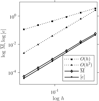
(a) ${[\,e\,]\,}$ and $\overline{\mathrm{M}}$

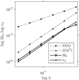
(b) ${e}_{\mathrm{d}}$ and $\overline{\mathrm{m}}_{\mathrm{d}}$

Figure 3: Ex. 1. The optimal convergence test of $\overline{\mathrm{m}}_{\mathrm{d}}$ and $\overline{\mathrm{M}}$.

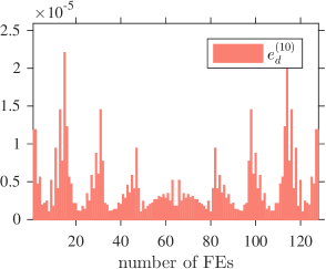
(a) $Q^{(10)}$: 128 EL, $\mathcal{T}_{9\times 9}$
${e}^{({10})}_{\mathrm{d}}=5.60\cdot 10^{-4}$

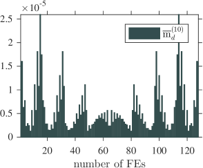
(b) $Q^{(10)}$: 128 EL, $\mathcal{T}_{9\times 9}$
$\overline{\mathrm{m}}^{({10})}_{\mathrm{d}}=7.46\cdot 10^{-4}$

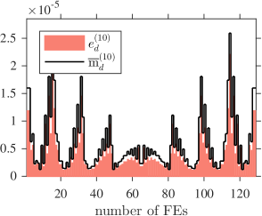
(c) $Q^{(10)}$: 128 EL
${e}^{({10})}_{\mathrm{d}}$ and $\overline{\mathrm{m}}^{({10})}_{\mathrm{d}}$ overlapped

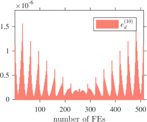
(d) $Q^{(10)}$: 512 EL, $\mathcal{T}_{17\times 17}$
${e}^{({10})}_{\mathrm{d}}=1.36\cdot 10^{-4}$

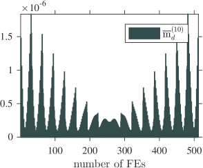
(e) $Q^{(10)}$: 512 EL, $\mathcal{T}_{17\times 17}$
$\overline{\mathrm{m}}^{({10})}_{\mathrm{d}}=1.88\cdot 10^{-4}$

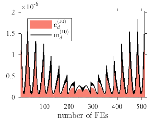
(f) $Q^{(10)}$: 512 EL
${e}^{({10})}_{\mathrm{d}}$ and $\overline{\mathrm{m}}^{({10})}_{\mathrm{d}}$ overlapped

Figure 4: Ex. 1. Distribution of the energy part of the error and the indicator on the slice $Q^{(10)}$.

Next, we solve the above formulated problem numerically with a fixed mesh on each time-step and confirm that $\overline{\mathrm{m}}^{({k})}_{\mathrm{d}}$ represents the local distribution of ${e}^{({k})}_{\mathrm{d}}$ efficiently on each $Q^{(k)}$. We fix two different meshes $\Theta_{10\times 18}$ (Figures 4a–4b) and $\Theta_{10\times 289}$ (Figures 4d–4e), where number of subintervals for discretisation in time is chosen as $K=10$. We compare the distributions of ${e}^{({10})}_{\mathrm{d}}$ and $\overline{\mathrm{m}}^{({10})}_{\mathrm{d}}$ on the final slice $Q^{(10)}$ for both meshes. Here, Figures 4a and 4d (first column) present the local distribution of ${e}^{({10})}_{\mathrm{d}}$ and Figures 4b and 4e(second column) illustrate the same element-wise characteristics for $\overline{\mathrm{m}}^{({10})}_{\mathrm{d}}$ (vertical axis), whereas the cell-elements (EL) are enumerated according to the FE implementation and depicted on the horizontal axis. Figures 4c and 4f illustrate the same distributions compared (overlapped) in a single graphic. For both cases, the histograms should convince the reader of the quantitative efficiency of the tested error indicator.

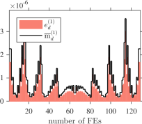
(a) $Q^{(1)}$: 128 EL
${e}^{({1})}_{\mathrm{d}}=7.54\cdot 10^{-5}$, $\overline{\mathrm{m}}^{({1})}_{\mathrm{d}}=1.02\cdot 10^{-4}$

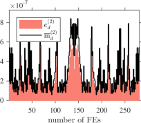
(b) $Q^{(2)}$: 280 EL
${e}^{({2})}_{\mathrm{d}}=6.09\cdot 10^{-5}$, $\overline{\mathrm{m}}^{({2})}_{\mathrm{d}}=7.64\cdot 10^{-5}$

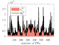
(c) $Q^{(3)}$: 688 EL
${e}^{({3})}_{\mathrm{d}}=3.16\cdot 10^{-5}$, $\overline{\mathrm{m}}^{({3})}_{\mathrm{d}}=3.80\cdot 10^{-5}$

Figure 5: Ex. 1. True error and indicator distribution on $Q^{(k)}$, $k=1,2,3$, (bulk marking $\mathbb{M}_{0.3}$).

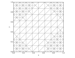
(a) $Q^{(1)}$:   276 EL, 165 ND
${e}^{({1})}_{\mathrm{d}}=7.97\cdot 10^{-5},\overline{\mathrm{m}}^{({1})}_{\mathrm{d}}=1.02\cdot 10^{-4}$

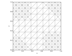
(b) $Q^{(1)}$:   280 EL, 167 ND
${e}^{({1})}_{\mathrm{d}}=6.52\cdot 10^{-5},\overline{\mathrm{m}}^{({1})}_{\mathrm{d}}=6.56\cdot 10^{-5}$

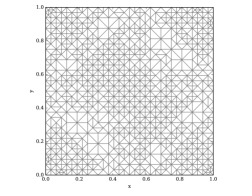
(c) $Q^{(3)}$:   1544 EL, 825 ND
${e}^{({3})}_{\mathrm{d}}=2.47\cdot 10^{-5},\overline{\mathrm{m}}^{({3})}_{\mathrm{d}}=2.44\cdot 10^{-5}$

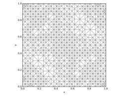
(d) $Q^{(3)}$:   1580 EL, 843 ND
${e}^{({3})}_{\mathrm{d}}=2.50\cdot 10^{-5},\overline{\mathrm{m}}^{({3})}_{\mathrm{d}}=2.47\cdot 10^{-5}$

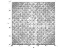
(e) $Q^{(5)}$:   8819 EL, 4541 ND
${e}^{({5})}_{\mathrm{d}}=7.48\cdot 10^{-6},\overline{\mathrm{m}}^{({5})}_{\mathrm{d}}=7.48\cdot 10^{-6}$

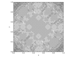
(f) $Q^{(5)}$:   9044 EL, 4649 ND
${e}^{({5})}_{\mathrm{d}}=7.49\cdot 10^{-6}$, $\overline{\mathrm{m}}^{({5})}_{\mathrm{d}}=7.49\cdot 10^{-6}$

Figure 6: Ex. 1. Evolution of meshes on the time-slices $Q^{(k)}$, $k=1,3,5$. The refinement is based on the true error (a), (c), (e) and the indicator (b), (d), (f) (bulk marking $\mathbb{M}_{0.3}$).

​

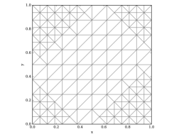
(a) $Q^{(1)}$:   284 EL,169 ND
${e}^{({1})}_{\mathrm{d}}=7.97\cdot 10^{-5},\overline{\mathrm{m}}^{({1})}_{\mathrm{d}}=1.02\cdot 10^{-4}$

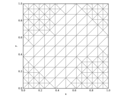
(b) $Q^{(1)}$:   296 EL, 175 ND
${e}^{({1})}_{\mathrm{d}}=7.97\cdot 10^{-5},\overline{\mathrm{m}}^{({1})}_{\mathrm{d}}=1.02\cdot 10^{-5}$

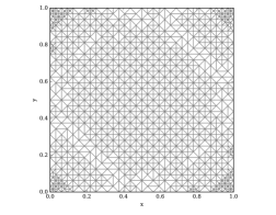
(c) $Q^{(3)}$:   2012 EL, 1065 ND
${e}^{({3})}_{\mathrm{d}}=3.18\cdot 10^{-5},\overline{\mathrm{m}}^{({3})}_{\mathrm{d}}=3.60\cdot 10^{-5}$

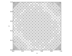
(d) $Q^{(3)}$:   2000 EL, 1057 ND
${e}^{({3})}_{\mathrm{d}}=3.08\cdot 10^{-5},\overline{\mathrm{m}}^{({3})}_{\mathrm{d}}=3.49\cdot 10^{-5}$

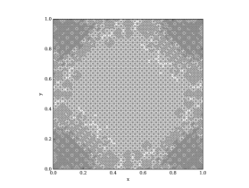
(e) $Q^{(5)}$:   13832 EL, 7059 ND
${e}^{({5})}_{\mathrm{d}}=6.91\cdot 10^{-6},\overline{\mathrm{m}}^{({5})}_{\mathrm{d}}=8.15\cdot 10^{-6}$

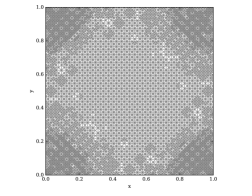
(f) $Q^{(5)}$:   13752 EL, 7027 ND
${e}^{({5})}_{\mathrm{d}}=6.94\cdot 10^{-6},\overline{\mathrm{m}}^{({5})}_{\mathrm{d}}=5.17\cdot 10^{-6}$

Figure 7: Ex. 1. Evolution of meshes on the time-slices $Q^{(k)}$, $k=1,3,5$. The refinement is based on the true error (a), (c), (e) and the indicator (b), (d), (f) using the marker $\mathbb{M}_{\rm AVR}$.

As a next step, we consider an adaptive refinement strategy with the bulk marking criterion $\mathbb{M}_{\theta}$ introduced in [9]. In this strategy, we form a subset of elements, which contain the highest indicated errors. The subset is formed in such a way that we keep adding elements until the accumulated error is reached. The selection process stops, when the error accumulated on the previous step exceeds the defined ‘bulk’ level (threshold). In this example, we set $\theta=0.3$ (for more details on alternative marking strategies, we refer the reader to [25]). Let the initial mesh be $\mathcal{T}_{121}$ (200 EL, 121 ND). Figure 5 illustrates the distributions of ${e}^{({k})}_{\mathrm{d}}$ and $\overline{\mathrm{m}}^{({k})}_{\mathrm{d}}$ on different cylinder slices $Q^{(k)}$, $k=1,2,3$, and demonstrates the quantitative efficiency of the indicator provided by the majorant. Under every sub-plot of Figure 5, we also provide the information on total values of ${e}^{({k})}_{\mathrm{d}}$ and $\overline{\mathrm{m}}^{({k})}_{\mathrm{d}}$.

We analyse the meshes obtained during the refinement based on either ${e}^{({k})}_{\mathrm{d}}$ or $\overline{\mathrm{m}}^{({k})}_{\mathrm{d}}$ (Figure 6a). In Figures 6a, 6c, and 6e (left column), we present the meshes obtained after the refinement process based on the local true error distribution, and Figures 6b, 6d, and 6f (right column) expose the meshes constructed when the refinement is based on the local indicator $\overline{\mathrm{m}}^{({k})}_{\mathrm{d}}$. It is easy to observe that the topology of the meshes on the RHS of Figure 6a resembles the topology of the meshes on the LHS. For this case, the efficiency of the total majorant is $I_{\rm eff}=1.23$.

The bulk marking strategy can be compared to marking determined by the level of the average error $\mathbb{M}_{\rm AVR}$ [25, Algorithm 2.1]. The latter one marks those elements, on which the error exceeds the average level. Figure 7 demonstrates the sequence of the meshes obtained as a result of the refinement based on ${e}^{({k})}_{\mathrm{d}}$ (LHS) and $\overline{\mathrm{m}}^{({k})}_{\mathrm{d}}$ (RHS) on the respective slices $Q^{(k)}$, $k=1,3,5$. In this case, we obtain the efficiency $I_{\rm eff}=1.4$. The majorant is not as accurate as expected, due to the fact that, unlike in the error majorants for the elliptic BVP, there is always a gap between $\overline{\mathrm{M}}$ and ${[\,e\,]\,}$ caused by the term $v_{t}$ in $\overline{\mathrm{m}}_{\mathrm{eq}}$ (see also (20)).

	Implicit scheme				Explicit scheme
$k$	DOFs$({v})$	${[\,e\,]\,}$	$\overline{\mathrm{M}}$	$I_{\rm eff}$	DOFs$({v})$	${[\,e\,]\,}$	$\overline{\mathrm{M}}$	$I_{\rm eff}$
1	14641	$2.29\cdot 10^{-9}$	$3.78\cdot 10^{-9}$	1.29	14641	$1.26\cdot 10^{-6}$	$7.89\cdot 10^{-5}$	7.93
2	23627	$4.01\cdot 10^{-9}$	$6.84\cdot 10^{-9}$	1.31	27175	$2.06\cdot 10^{-3}$	$4.56\cdot 10^{-3}$	1.49
3	39795	$5.05\cdot 10^{-9}$	$9.14\cdot 10^{-9}$	1.35	45489	$9.19\cdot 10^{3}\;\;$	$1.46\cdot 10^{4}\;\;$	1.26
4	67719	$5.66\cdot 10^{-9}$	$1.06\cdot 10^{-8}$	1.37	82344	$1.15\cdot 10^{12}$	$1.63\cdot 10^{12}$	1.19

Table 1: Ex. 1. Total error, majorant, and efficiency index for $v$ generated by implicit and explicit schemes.

It is important to note that the majorant can be used as a tool to predict the ‘blow-ups’ in time-dependent explicit schemes, which are less time-consuming in comparison to the implicit ones, but are unstable. Furthermore, if for one-dimensional (in space) schemes, the stability condition is written explicitly, for two- and three-dimensional problems as well as for non-linear problems there are no such criteria. As an example, we consider the mesh $\Theta_{1280\times 14641}$ (28800 EL, 14641 ND) and illustrate the majorant response on the instability of the explicit scheme (see Table 1). Here, the column DOFs$({v})$ reflects the number of DOFs for $v$. The LHS of the table contains total values of the error and the majorant, obtained by using a stable implicit scheme, whereas the RHS illustrates a drastic increase of the majorant even when the ‘blow-up’ is not yet obvious from the error values.

Example 2

In order to demonstrate that the same behaviour of the error estimates can be observed for the problems in higher dimension, we consider the unit cube $\Omega=(0,1)^{3}\subset{\mathds{R}}^{3}$ with $T=1$, $A=I$, $\boldsymbol{b}={\boldsymbol{0}}$, $c=0$, initial condition $u_{0}=x\,(1-x)\,y\,(1-y)\,z\,(1-z)$, homogeneous Dirichlet BC, and

$$u=x\,(1-x)\,y\,(1-y)\,z\,(1-z)(t^{2}+t+1).$$

Analogously, we take $v\in{\rm P}_{1}$. However, in the current example, we compare performance of the majorant reconstructed with two different approximations of the flux, i.e., approximated by Raviart-Thomas FEs of the lowest order $\boldsymbol{y}\in{\rm RT}_{0}$ and a linear one $\boldsymbol{y}\in{\rm RT}_{1}$. Figure 8a demonstrates the uniform convergence of ${[\,e\,]\,}$ and $\overline{\mathrm{M}}(\boldsymbol{y})$ with $\boldsymbol{y}\in{\rm RT}_{0}$, and Figure 8b depicts the same characteristics for $\boldsymbol{y}\in{\rm RT}_{1}$. They both confirm the optimal convergence order of the majorant constructed with $\boldsymbol{y}\in{\rm RT}_{0}$ and $\boldsymbol{y}\in{\rm RT}_{1}$.

(a) ${[\,e\,]\,}$, $\overline{\mathrm{M}}(\boldsymbol{y})$, $\boldsymbol{y}\in{\rm RT}_{0}$

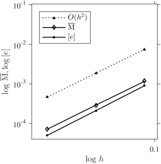
(b) ${[\,e\,]\,}$, $\overline{\mathrm{M}}(\boldsymbol{y})$, $\boldsymbol{y}\in{\rm RT}_{1}$

Figure 8: Ex. 2. The optimal convergence of $[e]$ and $\overline{\mathrm{M}}$, (a) $\boldsymbol{y}\in{\rm RT}_{0}$ and (b) $\boldsymbol{y}\in{\rm RT}_{1}$.

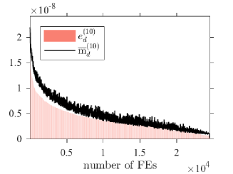
(a) $Q^{(10)}$: 24576 EL (sorted)
${e}^{({10})}_{\mathrm{d}}=9.13\cdot 10^{-5}$, $\overline{\mathrm{m}}^{({10})}_{\mathrm{d}}=1.16\cdot 10^{-4}$

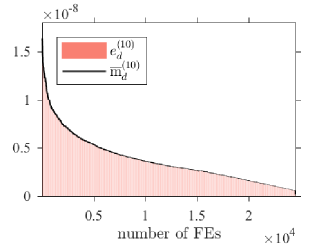
(b) $Q^{(10)}$: 24576 EL (sorted)
${e}^{({10})}_{\mathrm{d}}=9.13\cdot 10^{-5}$, $\overline{\mathrm{m}}^{({10})}_{\mathrm{d}}=9.15\cdot 10^{-5}$

Figure 9: Ex. 2. Energy parts of the true error and the indicator distributions based on (a) $\boldsymbol{y}\in{\rm RT}_{0}$ and (b) $\boldsymbol{y}\in{\rm RT}_{1}$.

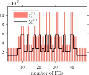
(a) $Q^{(0)}$: 48 EL
${e}^{({0})}_{\mathrm{d}}=2.10\cdot 10^{-2}$, $\overline{\mathrm{M}}^{(k)}{0}=8.43\cdot 10^{-3}$

(b) $Q^{(1)}$: 274 EL
${e}^{({1})}_{\mathrm{d}}=1.14\cdot 10^{-1}$, $\overline{\mathrm{M}}^{(k)}{1}=7.38\cdot 10^{-2}$

Figure 10: Ex. 2. Error and indicator distributions for the time-slices $Q^{(k)}$, $k=0,1$ ($\boldsymbol{y}\in{RT}_{1}$).

​​​​​​​​​

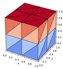
(a) $Q^{(0)}$: 48 EL

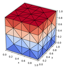
(b) $Q^{(1)}$: 356 EL

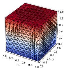
(c) $Q^{(3)}$: 5678 EL

Figure 11: Ex. 2. Evolution of meshes on the time-slices $Q^{(k)}$, $k=0,1,2,3$, the refinement is based on the majorant using the marker $\mathbb{M}_{\rm 0.6}$.

Next, we compare the indicators that are reconstructed based on the fluxes, approximated with elements of different degrees, i.e., ${\rm RT}_{0}$ and ${\rm RT}_{1}$. Figure 9a presents the error distributions and the error indicator on the same plot, but (unlike previous histograms) the arrays of cells are sorted such that the values of the local true errors ${e}^{({10})}_{\mathrm{d}}$ decrease. The array with $\overline{\mathrm{m}}^{({10})}_{\mathrm{d}}$ is depicted in the order defined by the indices obtained as a result of sorting. The evaluation of the error and the indicator distributions by such histograms was introduced in [25, Section 3.4]. It is easy to see that $\overline{\mathrm{m}}^{({10})}_{\mathrm{d}}$ (see Figure 9a) is less efficient than the one reconstructed from $\boldsymbol{y}\in{\rm RT}_{1}$ in Figure 9b. Latter illustrations reaffirm that using the fluxes of higher regularity is more advantageous for the majorant reconstruction, i.e., it guarantees a rather sharp and efficient prediction of the local error distribution.

Finally, we consider the refinement strategy with bulk marking $\mathbb{M}_{0.6}$. We take the initial mesh $\mathcal{T}_{3\times 3}$, $K=10$, and illustrate the obtained distributions after the refinement on the time-slices $k=0,1$ (Figure 11). The number of obtained elements and total values of ${e}^{({k})}_{\mathrm{d}}$ and $\overline{\mathrm{m}}^{({k})}_{\mathrm{d}}$ are pycharmshown below the plots. The evolution of meshes (obtained during the adaptation procedure from one slice to another, $k=0,1,3$) is shown in Figure 11.

Example 3

When the question of the efficient error indication is concerned, it is important to demonstrate that the studied majorant efficiently catches the error-jumps related to various singularities. One of the classical benchmark examples for such kind of testing is the problem defined on the $L$-shaped domain $\Omega:=(\scalebox{0.5}[1.0]{$-$}1,1)\times(\scalebox{0.5}[1.0]{$-$}1,1)\backslash[0,1)\times[0,\scalebox{0.5}[1.0]{$-$}1)$ with $T=1$, $A=I$, $\boldsymbol{b}={\boldsymbol{0}}$, $c=0$, the Dirichlet BC with the load $u_{D}=r^{1/3}\,\sin\theta$ with $r=(x^{2}+y^{2})$ and $\theta=\tfrac{2}{3}\,{\rm atan2}(y,x)$ on $\Sigma$, the input source function $f=r^{1/3}\,\sin\theta\,\left(2\,t+1\right)$, and the initial condition $u_{0}=r^{1/3}\,\sin\theta$. The corresponding exact solution $u=r^{1/3}\,\sin\theta\,\left(t^{2}+t+1\right)$ has a singularity at the point $(r,\theta)=(0,0)$.

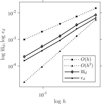
(a) ${e}_{\mathrm{d}}$ and $\overline{\mathrm{m}}_{\mathrm{d}}$

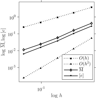
(b) ${[\,e\,]\,}$ and $\overline{\mathrm{M}}$

Figure 12: Ex. 3. The optimal convergence rate of ${e}_{\mathrm{d}}$ and $\overline{\mathrm{m}}_{\mathrm{d}}$ (a) and ${[\,e\,]\,}$ and $\overline{\mathrm{M}}$ (b).

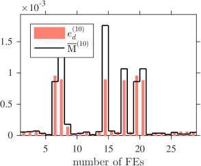
(a) $Q^{(10)}$: 28 EL
${e}^{({10})}_{\mathrm{d}}=2.46\cdot 10^{-3}$, $\overline{\mathrm{m}}^{({10})}_{\mathrm{d}}=3.50\cdot 10^{-3}$

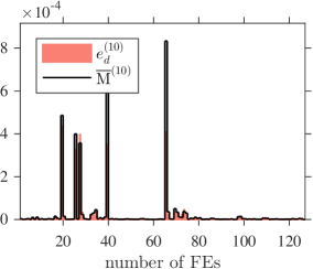
(b) $Q^{(10)}$: 192 EL
${e}^{({10})}_{\mathrm{d}}=2.46\cdot 10^{-3}$, $\overline{\mathrm{m}}^{({10})}_{\mathrm{d}}=3.50\cdot 10^{-3}$

Figure 13: Ex. 3. Error and indicator distributions on $Q^{(10)}$, computed on a mesh with (a) 28 EL and (b) 192 EL.

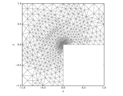
(a) $Q^{(5)}$:   1188 EL, 629 DOF
${e}^{({5})}_{\mathrm{d}}=7.78\cdot 10^{-4}$, $\overline{\mathrm{m}}^{({5})}_{\mathrm{d}}=1.00\cdot 10^{-3}$

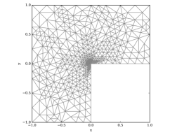
(b) $Q^{(5)}$:   1022 EL, 543 DOF
${e}^{({5})}_{\mathrm{d}}=8.35\cdot 10^{-3}$, $\overline{\mathrm{m}}^{({5})}_{\mathrm{d}}=1.07\cdot 10^{-3}$

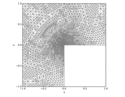
(c) $Q^{(7)}$:   5846 EL, 3008 DOF
${e}^{({7})}_{\mathrm{d}}=3.04\cdot 10^{-4}$, $\overline{\mathrm{m}}^{({7})}_{\mathrm{d}}=3.43\cdot 10^{-4}$

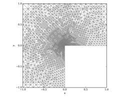
(d) $Q^{(7)}$:   4676 EL, 2400 DOF
${e}^{({7})}_{\mathrm{d}}=3.45\cdot 10^{-4}$, $\overline{\mathrm{m}}^{({7})}_{\mathrm{d}}=3.88\cdot 10^{-4}$

Figure 14: Ex. 3. Evolution of meshes on $Q^{(k)}$, $k=5,7$, after the refinements based on the true error (a), (c) and on the indicator (b), (d), using the marking $\mathbb{M}_{\rm AVR}$.

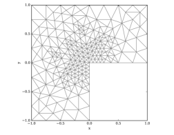
(a) $Q^{(3)}$:   470 EL, 256 ND
${e}^{({3})}_{\mathrm{d}}=1.88\cdot 10^{-3}$, $\overline{\mathrm{m}}^{({3})}_{\mathrm{d}}=2.44\cdot 10^{-3}$

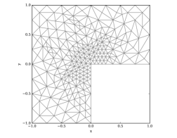
(b) $Q^{(3)}$:   489 EL, 266 ND
${e}^{({3})}_{\mathrm{d}}=1.80\cdot 10^{-3}$, $\overline{\mathrm{m}}^{({3})}_{\mathrm{d}}=2.35\cdot 10^{-3}$

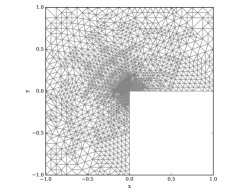
(c) $Q^{(5)}$:   3013 EL, 1563 ND
${e}^{({5})}_{\mathrm{d}}=5.34\cdot 10^{-4}$, $\overline{\mathrm{m}}^{({5})}_{\mathrm{d}}=7.12\cdot 10^{-4}$

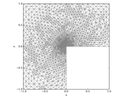
(d) $Q^{(5)}$:   3055 EL, 1579 ND
${e}^{({5})}_{\mathrm{d}}=5.36\cdot 10^{-4}$, $\overline{\mathrm{m}}^{({5})}_{\mathrm{d}}=7.11\cdot 10^{-4}$

​
​

Figure 15: Ex. 3. Evolution of meshes on $Q^{(k)}$, $k=3,5$, after the refinement based on the true error (a), (c) and on the indicator (b), (d), using bulk marking $\mathbb{M}_{0.3}$.

The results of the optimal convergence test for the indicator $\overline{\mathrm{m}}_{\mathrm{d}}$ are provided in Figure 12a (taking into account that $v\in{\rm P}_{1}$ and $\boldsymbol{y}\in{\rm RT}_{1}$). Analogously, we fix the time-step ($K=100$) and refine the mesh discretising $\Omega$. As expected, the speed of convergence of both the error and the majorant is suboptimal and lies between $O(h)$ and $O(h^{2})$. Figure 12b provides the plot illustrating the convergence of the total error and the majorant. The difference in the decay of $\overline{\mathrm{m}}_{\mathrm{d}}$ and $\overline{\mathrm{M}}$ can be explained by the presence of the term $-v_{t}$ in $\overline{\mathrm{m}}_{\mathrm{eq}}$ (the equilibrium part of the majorant) and possible accumulation of the error in the flux $\boldsymbol{y}$ (in addition to the accumulation of the error in $v$).

Let $K=10$. Then, the distribution of the local errors on $Q^{(10)}$ is indicated quite efficiently by $\overline{\mathrm{m}}^{({10})}_{\mathrm{d}}$ (see Figure 13). Figure 13a provides information about the error and majorant distribution on $Q^{(10)}$, where $\Omega$ is discretised by the mesh with 28 EL. Figure 13b illustrates analogous characteristics for the refined mesh with 192 EL. Both figures confirm that $\overline{\mathrm{m}}^{({k})}_{\mathrm{d}}$ manages to locate the errors associated with solution singularities.

Finally, we consider the adaptive refinement with two marking procedures and analyse the obtained meshes. Figure 14 shows the meshes, obtained by using the marker $\mathbb{M}_{\rm AVR}$, and Figure 15 compares the meshes derived using the bulk marking $\mathbb{M}_{0.3}$. Analogously to Ex. 1, one can see that the meshes generated during the refinement based on the local true error distribution (LHS) are similar to the corresponding meshes provided by adaptive algorithm based on the local indicator (RHS).

In two final examples, we consider rather realistic cases, where the exact solution is not given explicitly and only the prescribed right-hand side and BC are known. In this setting, we compare the approximations reconstructed by ${\rm P}_{1}$ FEs to the reference solutions reconstructed with the Lagrangian polynomials of degree $4$. Naturally, such a comparison (without an exact solution) has only heuristic character, however, this is the only way to estimate the error in real-life problems.

Example 4

In the current example, let the domain have $\Pi$-shape, i.e.,

$$\Omega:=(-1,1)\times(-1,1)/\big{[}-\tfrac{1}{2},-\tfrac{1}{2}\big{]}\times[0,-1)\in{\mathds{R}}^{2},$$

with the final time fixed to $T=2$. We consider rather trivial initial and boundary conditions $u_{0}=0$ and $u_{D}=0$, and the coefficients in (4) are chosen the following way: $A=I$, $\boldsymbol{b}={\boldsymbol{0}}$, $c=0$. The source function

$$f=t\sin t\sin\pi x+t\cos t\sin\pi y,$$

rapidly oscillating on $Q$, produces approximations changing in time that are depicted in Figure 16. Here, the approximate solution is reproduced on the fixed mesh $\mathcal{T}_{h}$ (411 ND) and with $K=15$ time steps.

​​​​ ​

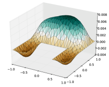
(a) $v^{1}\quad\mbox{on}\quad\Omega_{t^{1}}$

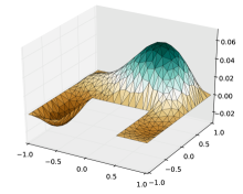
(b) $v^{5}\quad\mbox{on}\quad\Omega_{t^{5}}$

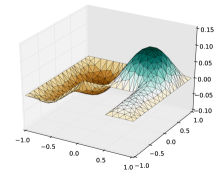
(c) $v^{11}\quad\mbox{on}\quad\Omega_{t^{11}}$

Figure 16: Ex. 4. Sequence of approximate solutions reconstructed on the mesh $\mathcal{T}_{h}$ (411 ND).

​​​​
​​​​

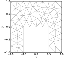
(a)   $Q^{(0)}$: initial mesh
110 EL, 76 ND

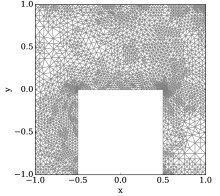
(b)   $Q^{(9)}$: refinement based on ${e}_{\mathrm{d}}$
    5923 EL, 3095 ND

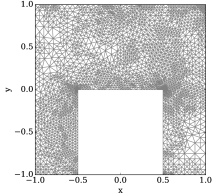
(c)   $Q^{(9)}$: refinement based on $\overline{\mathrm{m}}_{\mathrm{d}}$
    5828 EL, 3048 ND

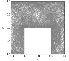
(d)   $Q^{(12)}$: refinement based on ${e}_{\mathrm{d}}$
    21158 EL, 10827 ND

(e)   $Q^{(12)}$: refinement based on $\overline{\mathrm{m}}_{\mathrm{d}}$
    21158 EL, 10828 ND

Figure 17: Ex. 4. Initial mesh (a) and the meshes produced during the refinement on $Q^{(9)}$ and $Q^{(12)}$ time-slabs based either on the true error (b), (d) or on the majorant (c), (e), using the bulk marking $\mathbb{M}_{0.1}$.

$Q^{(k)}$	$[e]_{\cup_{i=1}^{k}{Q^{(i)}}}$	$\overline{\mathrm{M}}_{\cup_{i=1}^{k}{Q^{(i)}}}$	$I_{\rm eff}=\overline{\mathrm{M}}_{\cup_{i=1}^{k}{Q^{(i)}}}/[e]_{\cup_{i=1}^{k}{Q^{(i)}}}$
$Q^{(0)}$	$4.23\cdot 10^{-6}$	$2.99\cdot 10^{-5}$	2.66
$Q^{(2)}$	$6.80\cdot 10^{-5}$	$1.18\cdot 10^{-4}$	1.32
$Q^{(4)}$	$1.90\cdot 10^{-4}$	$2.87\cdot 10^{-4}$	1.23
$Q^{(6)}$	$3.20\cdot 10^{-4}$	$4.68\cdot 10^{-4}$	1.21
$Q^{(8)}$	$4.26\cdot 10^{-4}$	$6.21\cdot 10^{-4}$	1.21
$Q^{(10)}$	$5.02\cdot 10^{-4}$	$7.37\cdot 10^{-4}$	1.21
$Q^{(12)}$	$5.49\cdot 10^{-4}$	$8.17\cdot 10^{-4}$	1.22
$Q^{(14)}$	$5.76\cdot 10^{-4}$	$8.69\cdot 10^{-4}$	1.23

Table 2: Ex. 4. Accumulation of the total error and the majorant.

As in previous examples, we test the efficiency of the error indicator (generated by the majorant) by comparing the meshes produced during the adaptive refinement steps performed based either on ${e}_{\mathrm{d}}$ or on $\overline{\mathrm{m}}_{\mathrm{d}}$. We use the bulk marking criterion with the parameter $\theta=0.1$ for selecting elements of the mesh that need to be refined. In Figure 19a, we present the initial mesh that is taken in both refinement procedures. Figure 19b illustrates the resulting mesh that is produced on the time-slice $Q^{(9)}$ after using to the true error distribution as the refinement criterion, and, finally, Figure 19c depicts the mesh corresponding to the refinements based on the error indicator element-wise distribution. Similar meshes are presented for the time-slice $Q^{(12)}$ in Figures 19d and 19e.

The total energy error and the majorant (accumulated incrementally as the time passes) are presented in Table 2. The first column contains sequential time-steps, the second one presents the error (including the error at previous $k\!-\!1$ steps as well as the increment ${e}^{({k})}_{\mathrm{d}}$ on the $k$-th interval), the third column corresponds to the majorant, and the last one shows the majorant efficiency index characterising its performance. It is obvious that in the current test-case, the efficiency index indicates the adequate behaviour of the majorant even though the source term $f$ strongly depends on $t$. This can be explained by looking closer at the error and the element-wise indicator distributions (see Figure 18). Here, Figures 18a–18d in the first row present the local error distributions w.r.t. numbered finite elements (the horizontal axis), whereas Figures 18e–18h illustrate the majorant element-wise distribution. One can see that the estimate mimics all local jumps of the errors not only qualitatively but also quantitatively sharp. That affects the efficiency index respectively, therefore it stays in the range of the interval $[1.21,1.23]$.

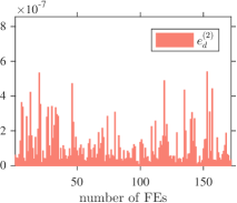
(a) ${e}^{({2})}_{\mathrm{d}}$

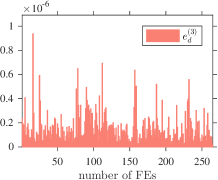
(b) ${e}^{({3})}_{\mathrm{d}}$

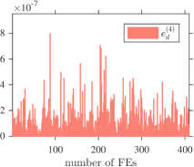
(c) ${e}^{({4})}_{\mathrm{d}}$

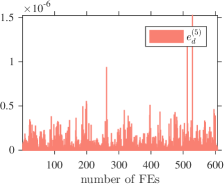
(d) ${e}^{({5})}_{\mathrm{d}}$

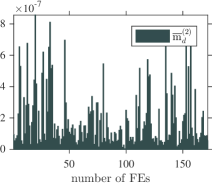
(e) $\overline{\mathrm{m}}^{({2})}_{\mathrm{d}}$

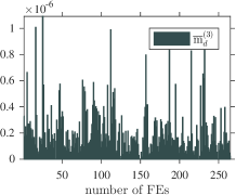
(f) $\overline{\mathrm{m}}^{({3})}_{\mathrm{d}}$

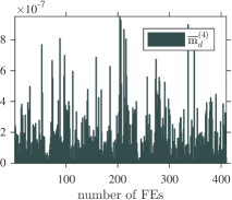
(g) $\overline{\mathrm{m}}^{({4})}_{\mathrm{d}}$

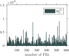
(h) $\overline{\mathrm{m}}^{({5})}_{\mathrm{d}}$

Figure 18: Ex. 4. Local distribution of the error ${e}^{({k})}_{\mathrm{d}}$ and the indicator $\overline{\mathrm{m}}^{({k})}_{\mathrm{d}}$, $k=2,3,4,5$.

Example 5

In the final example of the current section, we investigate the problem with a right-hand side that contains rapidly changing singularity in the source term

$$f=t\,\sin t\,e^{-100\,((y-0.8)^{2}+(x+0.8)^{2})}+t\,\cos t\,e^{-100\,((y-0.8)^{2}+(x-0.8)^{2})}.$$

The domain is defined by a curved $\Pi$-shape domain $\Omega:=(-1,1)\times(0,1)\backslash B_{{}^{1}\!/_{2}}(0,0)$, where $B_{{}^{1}\!/_{2}}(0,0)$ defines a circle of a radius $\tfrac{1}{2}$ with the centre at the point $(0,0)$. The operator is chosen as $A=\begin{bmatrix}1&0\\ 0&10\\ \end{bmatrix}$, $\boldsymbol{b}={\boldsymbol{0}}$, $c=0$, and the initial and boundary conditions are zero.

Because of the nature of FE discretisation and the semicircle-shaped boundary of $\Omega$, the spatial mesh does not exactly represents the domain. This implies that the error ($u-v$) is not exactly zero in curved part of the boundary. For that reason, the functional majorant is not applicable unless we project the error on the Dirichlet part of the boundary. However, both the majorant and the error indicator can be used in the heuristic sense.

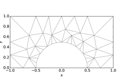
(a) $Q^{(0)}$: initial mesh, 56 EL, 45 ND

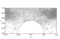
(b)   $Q^{(10)}$: refinement based on ${e}_{\mathrm{d}}$
    5923 EL, 3095 ND

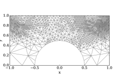
(c)   $Q^{(10)}$: refinement based on $\overline{\mathrm{m}}_{\mathrm{d}}$
    5828 EL, 3048 ND

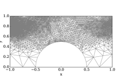
(d)   $Q^{(13)}$: refinement based on ${e}_{\mathrm{d}}$
    13551 EL, 6881 ND

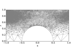
(e)   $Q^{(13)}$: refinement based on $\overline{\mathrm{m}}_{\mathrm{d}}$
    16664 EL, 8449 ND

Figure 19: Ex. 5. Initial mesh (a) and meshes produced during refinement based on the true error (b), (d) and the majorant (c), (e) on the time-slices $Q^{(10)}$ and $Q^{(13)}$, using bulk marking $\mathbb{M}_{0.1}$.

As it is expected, we see the mesh being refined over time at the singularity points of the domain $\Omega$, i.e., $(-0.8,-0.8)$ and $(-0.8,0.8)$ (Figure 19). Also, Table 3 confirms that despite of the singularities in the solution and the non-unitary operator $A$, the efficiency of the error estimates stays rather adequate, i.e., $I_{\rm eff}\in[1.89,3.77]$.

$Q^{(k)}$	$[e]_{\cup_{i=1}^{k}{Q^{(i)}}}$	$\overline{\mathrm{M}}_{\cup_{i=1}^{k}{Q^{(i)}}}$	$I_{\rm eff}=\overline{\mathrm{M}}_{\cup_{i=1}^{k}{Q^{(i)}}}/[e]_{\cup_{i=1}^{k}{Q^{(i)}}}$
$Q^{(0)}$	$3.45\cdot 10^{-6}$	$4.92\cdot 10^{-5}$	3.77
$Q^{(2)}$	$2.68\cdot 10^{-5}$	$1.58\cdot 10^{-4}$	2.43
$Q^{(4)}$	$7.36\cdot 10^{-5}$	$3.41\cdot 10^{-4}$	2.15
$Q^{(6)}$	$1.21\cdot 10^{-4}$	$5.45\cdot 10^{-4}$	2.12
$Q^{(8)}$	$1.57\cdot 10^{-4}$	$6.44\cdot 10^{-4}$	2.02
$Q^{(10)}$	$1.84\cdot 10^{-4}$	$6.98\cdot 10^{-4}$	1.95
$Q^{(12)}$	$2.02\cdot 10^{-4}$	$7.39\cdot 10^{-4}$	1.91
$Q^{(14)}$	$2.18\cdot 10^{-4}$	$7.77\cdot 10^{-4}$	1.89

Table 3: Ex. 5. Accumulation of the total error and the majorant.

4 Space-time approach

Due to main drawbacks of the incremental method (i.e., being time-consuming and complicated to parallelise), the space-time FEM approach has been developed. The simplest ideas for space-time solvers are based on time-parallel integration techniques for ordinary differential equations (ODEs) (an overview of the history of this approach can be found in [13]). Monograph [15] introduces a scheme that executes a multigrid method for the elliptic problem on each time-step, such that the time is treated as an $(d+1)$-th spatial direction in the space-time grid. Later, more space-time discretisation methods were suggested, i.e., the so-called parallel time-stepping method [46], the multigrid waveform relaxation method (space parallelism) [44, 24], and the full space-time multigrid method (using the Fourier mode analysis) [16]. Recently, due to appearance of powerful multi-core computers and advances in parallelised computational methods, application of space-time discretisation techniques became popular in various scientific and industrial applications (see, e.g., [41, 40, 42, 18], and the references therein). A comprehensive review on existing works in space-time techniques can be found in [22]. Since the majorant is defined as an integral over the whole space-time cylinder $Q$, this section contains clarifications on how to apply the optimisation algorithm in case of space-time discretisation techniques (see Algorithm 2). Numerical results obtained by testing the majorant w.r.t. this approach are exposed in Ex. 6 and 8.

When applying the majorant to the space-time schemes, where time is considered as an additional dimension, the optimality condition (26) yields the variational formulation on the whole $Q$, i.e.,

$$\tfrac{C_{{\rm F}\Omega}^{2}}{\beta\,\underline{\nu}_{A}}\,(\mathrm{div}_{x}\boldsymbol{y},\mathrm{div}_{x}\boldsymbol{w})_{Q}+(A^{-1}\boldsymbol{y},\boldsymbol{w})_{Q}=-\tfrac{C_{{\rm F}\Omega}^{2}}{\beta\,\underline{\nu}_{A}}\big{(}f-v_{t},\mathrm{div}_{x}\boldsymbol{w})_{Q}+(\nabla_{x}v,\boldsymbol{w})_{Q}.$$

In this case, $\boldsymbol{y},\boldsymbol{w}\in{\rm span}\,\big{\{}\,\boldsymbol{\varphi}_{1},...,\boldsymbol{\varphi}_{M}\big{\}}\subset H^{\mathrm{div}_{x}}(Q)$, i.e., $\boldsymbol{y}=\sum_{i=1}^{M}Y_{i}\,\boldsymbol{\varphi}_{i}$, where $Y\in{\mathds{R}}^{M}$ is a vector of degrees of freedom (DOFs) approximating $\boldsymbol{y}$, and the test function can be set to $\boldsymbol{w}=\boldsymbol{\varphi}_{j}$, $j=1,\ldots,M$. Then, Algorithm 2 of minimising the majorant follows the steps of Algorithm 3.2 in [25, Section 3.3.1]. The structure of Algorithm 2 is similar to the one for the incremental scheme with exception that refinement steps are carried out on the whole space-time domain $Q$ instead of the time-slices $Q^{(k)}$. In the current case, the adaptivity in time direction is automated since $t$ is treated as $x_{d+1}$-coordinate.

Algorithm 2  Global minimisation of $\overline{\mathrm{M}}$ (in the case of a space-time scheme)

  Input: $Q$: $v$ {approximate solution}

            $\boldsymbol{\varphi}_{i}$, $i=1,\ldots,M$ {$H^{\mathrm{div}_{x}}(Q)$-conforming basis functions}

            $L^{\rm iter}_{\rm max}$ {number of iterations}

  

  Assemble the matrices $\widetilde{S}$, $\widetilde{K}\in{\mathds{R}}^{M\times M}$ and the vectors $\widetilde{z}$, $\widetilde{g}\in{\mathds{R}}^{M}$ by using

$$\!\!\{\widetilde{S}_{ij}\}_{i,j=1}^{M} =(\mathrm{div}_{x}\boldsymbol{\varphi}_{i},\mathrm{div}_{x}\boldsymbol{\varphi}_{j})_{Q},\;\quad\{\widetilde{z}_{j}\}_{j=1}^{M}=\big{(}f-v_{t},\mathrm{div}_{x}\boldsymbol{\varphi}_{j}\big{)}_{Q},$$

$$\{\widetilde{K}_{ij}\}_{i,j=1}^{M} =(A^{-1}\boldsymbol{\varphi}_{i},\boldsymbol{\varphi}_{j})_{Q},\qquad\;\quad\{\widetilde{g}_{j}\}_{j=1}^{M}=\big{(}\nabla_{x}v,\boldsymbol{\varphi}_{j}\big{)}_{Q}.$$

  Initialise $\beta$, e.g., $\beta=1$.

  for $l=1$ to $L^{\rm iter}_{\rm max}$ do

     Solve the system  $\left(\tfrac{C_{{\rm F}\Omega}^{2}}{\beta\,\underline{\nu}_{A}}\widetilde{S}+\widetilde{K}\right)\,{Y}=-\tfrac{C_{{\rm F}\Omega}^{2}}{\beta\,\underline{\nu}_{A}}\widetilde{z}+\widetilde{g}.$

     Approximate the flux $\boldsymbol{y}=\sum\limits_{i=1}^{M}Y_{i}\boldsymbol{\varphi}_{i}$.

     Compute the components of the majorant by using

$$\overline{\mathrm{m}}_{\mathrm{eq}}:=\|\,f+\mathrm{div}_{x}\boldsymbol{y}-v_{t}\,\|^{2}_{Q}\quad\mbox{and}\quad\overline{\mathrm{m}}_{\mathrm{d}}:=\|\boldsymbol{y}-A\nabla_{x}v\,\|^{2}_{A^{-1},Q}.$$

     Compute the optimal $\beta$ by using $\beta:=\left(\tfrac{C_{{\rm F}\Omega}^{2}\overline{\mathrm{m}}_{\mathrm{eq}}}{\underline{\nu}_{A}\overline{\mathrm{m}}_{\mathrm{d}}}\right)^{{}^{1}\!/_{2}}.$

  end for

  Compute the majorant by using

$$\overline{\mathrm{M}}(v,\boldsymbol{y};\beta):=(1+\beta)\,\|\boldsymbol{y}-A\nabla_{x}v\,\|^{2}_{A^{-1},Q}+(1+\tfrac{1}{\beta})\,\tfrac{C_{{\rm F}\Omega}^{2}}{\underline{\nu}_{A}}\|\,f+\mathrm{div}_{x}\boldsymbol{y}-v_{t}\,\|^{2}_{Q}.$$

  Output: $\overline{\mathrm{M}}(v,\boldsymbol{y};\beta)$ {majorant on $Q$}

Example 6

First, let us consider the numerical properties of $\overline{\mathrm{M}}$ and the corresponding indicator on the unit interval $\Omega=(0,1)\subset{\mathds{R}}$, $T=1$, $A=I$, $\boldsymbol{b}={\boldsymbol{0}}$, $c=0$, and homogeneous Dirichlet BC. The exact solution is $u=x\,(1-x)\,(t^{2}+t+1)$ with the IC being $u_{0}=x\,(1-x)$. The approximation is reconstructed by ${\rm P}_{1}$ FEs, and the flux is approximated by ${\rm P}_{2}$ FEs. In Figure 20, we confirm the order of convergence $O(h^{2})$ for $\overline{\mathrm{M}}$ after several simultaneous refinement iterations (w.r.t. space and time).

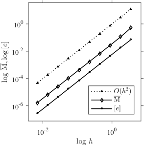
Figure 20: Ex. 6. The optimal convergence of the total error and majorant.

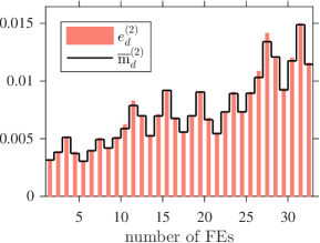
(a) 2 REF: 32 EL,
${e}_{\mathrm{d}}=9.11\cdot 10^{-2},\overline{\mathrm{m}}_{\mathrm{d}}=9.16\cdot 10^{-1}$

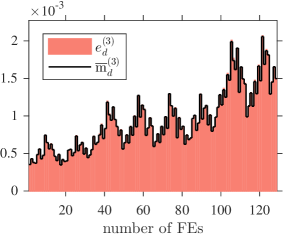
(b) 3 REF: 128 EL,
${e}_{\mathrm{d}}=2.30\cdot 10^{-2},\overline{\mathrm{m}}_{\mathrm{d}}=2.30\cdot 10^{-2}$

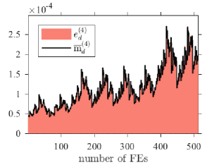
(c) 4 REF: 512 EL,
${e}_{\mathrm{d}}=1.44\cdot 10^{-3},\overline{\mathrm{m}}_{\mathrm{d}}=1.44\cdot 10^{-3}$

​ ​

Figure 21: Ex. 6. ${e}_{\mathrm{d}}$ and $\overline{\mathrm{m}}_{\mathrm{d}}$ distributions after REF $\#=2,3,4$.

Next, we consider the true error and majorant distributions obtained on each refinement step starting from the initial mesh $\mathcal{T}_{3\times 3}$ (see Figure 21). In Figures 21a–21c, we illustrate ${e}_{\mathrm{d}}$ and $\overline{\mathrm{m}}_{\mathrm{d}}$ after the refinement steps (REF) 2, 3, 4, 5, respectively. Here, the elements are ordered by the certain numbering procedure in FE code implementation. The graphs confirm that the indicator indeed manages to mimic the error distribution and to catch local jumps of the error very efficiently. Table 4 confirms the efficiency of the total majorant.

$\#$ REF	$\#$ EL	${[\,e\,]\,}$	$\overline{\mathrm{M}}$	$I_{\rm eff}$
1	8	$3.5229\cdot 10^{-1}$	$4.0889\cdot 10^{-1}$	1.08
3	128	$2.2969\cdot 10^{-2}$	$2.7215\cdot 10^{-2}$	1.09
5	2048	$1.4393\cdot 10^{-3}$	$1.7209\cdot 10^{-3}$	1.09
7	131072	$2.2493\cdot 10^{-5}$	$2.6969\cdot 10^{-5}$	1.09
9	2097152	$1.4058\cdot 10^{-6}$	$1.6861\cdot 10^{-6}$	1.10

Table 4: Ex. 6. Total error, majorant, and efficiency index w.r.t. refinement steps.

Example 7

Let us consider the same problem discussed in Ex. 1 by the space-time discretisation scheme. The used FE spaces are as follows: $v\in{\rm P}_{1}$ and $\boldsymbol{y}\in{\rm P}_{2}$. We consider two meshes obtained after the uniform refinement on the steps REF 1, 2 (see Figures 22a–22b). Again, the local error and the indicator distributions are shown element-wise. Table 5 provides information about the efficiency index of the majorant on every REF, which improved on average by $20\%$ in comparison to the time-stepping approach.

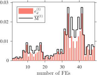
(a) 1 REF: 48 EL
${e}_{\mathrm{d}}=4.77\cdot 10^{-2},\overline{\mathrm{M}}=5.60\cdot 10^{-2}$

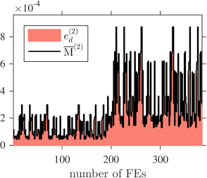
(b) 2 REF: 384 EL
${e}_{\mathrm{d}}=1.73\cdot 10^{-2},\overline{\mathrm{M}}=1.92\cdot 10^{-2}$

Figure 22: Ex. 7. Distribution of the error and the majorant after refinement steps $\#=1,2$.

$\#$ REF	$\#$ EL	${[\,e\,]\,}$	$\overline{\mathrm{M}}$	$I_{\rm eff}$
1	48	$4.7719\cdot 10^{-2}$	$5.6030\cdot 10^{-2}$	1.08
2	384	$1.7268\cdot 10^{-2}$	$1.9175\cdot 10^{-2}$	1.05
3	3072	$8.4558\cdot 10^{-3}$	$9.4992\cdot 10^{-3}$	1.06
4	24576	$6.1427\cdot 10^{-3}$	$6.9789\cdot 10^{-3}$	1.07
5	196608	$5.5479\cdot 10^{-3}$	$6.2617\cdot 10^{-3}$	1.06

Table 5: Ex. 7. Total error, the majorant, and the efficiency index w.r.t. to refinement steps.

Example 8

Finally, we construct an example with dissipating exact solution and zero RHS and investigate how the parameter $\sigma$ affects the quality of the error indication. This example demonstrates also the automated adaptive strategy suggested by the majorant. The initial condition $u_{0}=6\,\sin\pi x$ determines the solution $u=6\,\sin\pi x\,e^{-\tfrac{\pi^{2}t}{\sigma}}$. For different $\sigma$, one obtains the solutions presented in Figure 23.

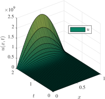
(a) $\sigma=1$

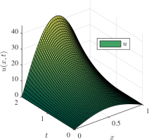
(b) $\sigma=10$

Figure 23: Ex. 8. Exact solutions for $\sigma=1$ and $10$.

Assume first that $\sigma=1$. Let the number of refinements be ${\rm REF}=12$ and the bulk marking procedure have the parameter $\theta=0.3$. Having compared the meshes obtained while refining based on the error (Figures 24a–24d) and the majorant distribution (Figures 24b–24d), one observes that the majorant adequately detects the region of large gradients in the solution. Using the true error for the refinement, we obtain the following $L^{2}$ and energy norms of errors: $\|e\|^{2}_{Q}=3.56\cdot 10^{-7}$ and $\|\nabla_{x}e\|^{2}_{Q}=2.02\cdot 10^{-2}$. Whereas, the refinement based on $\overline{\mathrm{m}}_{\mathrm{d}}$ results into the errors $\|e\|^{2}_{Q}=3.56\cdot 10^{-7}$ and $\|\nabla_{x}e\|^{2}_{Q}=2.02\cdot 10^{-2}$. The efficiency index obtained after $12$ refinement steps equals to $1.25$, which is quite adequate number taking into account the jump in the exact solution.

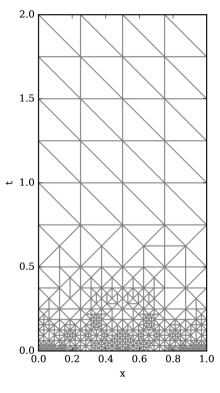
(a) REF $\#$ 4: $\mbox{based on}\;{e}_{\mathrm{d}}$
796 EL, 440 ND

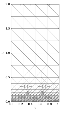
(b) REF $\#$ 4: $\mbox{based on}\;\overline{\mathrm{m}}_{\mathrm{d}}$
776 EL, 431 ND

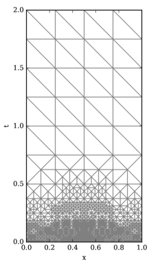
(c) REF $\#$ 6: $\mbox{based on}\;{e}_{\mathrm{d}}$
3340 EL, 1739 ND

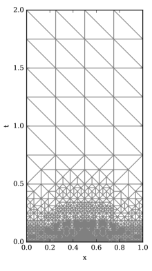
(d) REF $\#$ 6: $\mbox{based on}\;\overline{\mathrm{m}}_{\mathrm{d}}$
3374 EL, 1758 ND

​
​

Figure 24: Ex. 8 for $\sigma=1$. Space-time refinement based on the true energy error (a), (c) and on the majorant (b), (d) using the bulk marker $\mathbb{M}_{0.3}$.

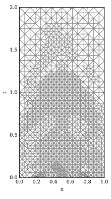
(a) REF $\#$ 6: $\mbox{based on}\;{e}_{\mathrm{d}}$
2548 EL, 1321 ND

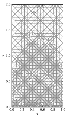
(b) REF $\#$ 6: $\mbox{based on}\;\overline{\mathrm{m}}_{\mathrm{d}}$
2660 EL, 1387 ND

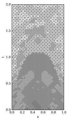
(c) REF $\#$ 8: $\mbox{based on}\;{e}_{\mathrm{d}}$
8706 EL, 4437 ND

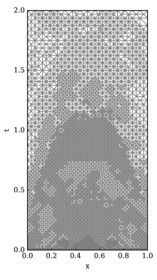
(d) REF $\#$ 8: $\mbox{based on}\;\overline{\mathrm{m}}_{\mathrm{d}}$
9274 EL, 4735 ND

​
​

Figure 25: Ex. 8 for $\sigma=10$. Space-time refinement based on the true energy error (a), (c) and on the majorant (b), (d) using the bulk marker $\mathbb{M}_{0.3}$.

$\#$ REF	$\#$ EL	${[\,e\,]\,}$	$\overline{\mathrm{M}}$	$I_{\rm eff}$
1	71	1.50	2.29	1.52
3	218	$8.35\cdot 10^{-1}$	1.10	1.31
5	881	$3.90\cdot 10^{-1}$	$4.97\cdot 10^{-1}$	1.27
7	3332	$2.02\cdot 10^{-1}$	$2.54\cdot 10^{-1}$	1.26
9	11538	$1.10\cdot 10^{-1}$	$1.38\cdot 10^{-1}$	1.26
11	38218	$6.28\cdot 10^{-2}$	$7.87\cdot 10^{-2}$	1.25

Table 6: Ex. 8 for $\sigma=1$. Total error, majorant, and efficiency index w.r.t. to refinement steps with the bulk marking $\theta=0.3$.

The same comparison of meshes is done for $\sigma=10$ in Figure 25. Table 7 illustrates that the efficiency index is affected by the value of $\sigma$ but still stays relatively adequate. For a lage $\sigma$, the reliability term of the majorant $\overline{\mathrm{m}}_{\mathrm{eq}}$ is more complicated to minimise due to the term $\sigma\,v_{t}$. In the space-time setting, it can be interpreted as a very strong convection term. In order to reduce the effect of $\overline{\mathrm{m}}_{\mathrm{eq}}$ on the global majorant, one needs to use more sophisticated methods (tailored to the convection-dominated problems), which are beyond the focus of this paper.

$\#$ REF	$\#$ EL	${[\,e\,]\,}$	$\overline{\mathrm{M}}$	$I_{\rm eff}$
1	71	1.55	3.18	2.05
3	219	$8.08\cdot 10^{-1}$	1.65	2.05
5	741	$4.28\cdot 10^{-1}$	$8.60\cdot 10^{-1}$	2.01
7	2557	$2.29\cdot 10^{-1}$	$4.72\cdot 10^{-1}$	2.06
9	8736	$1.23\cdot 10^{-1}$	$2.58\cdot 10^{-1}$	2.10
11	29501	$6.68\cdot 10^{-2}$	$1.39\cdot 10^{-1}$	2.09

Table 7: Ex. 8 for $\sigma=10$. Total error, majorant, and efficiency index w.r.t. to refinement steps with the bulk marking $\theta=0.3$.

5 Conclusion

In this paper, we have discussed guaranteed bounds of the distance to the exact solution of the evolutionary reaction-diffusion problem with the Dirichlet BC. We have shown that these error estimates are directly computable and rather efficient. The functional formulation of the estimates makes them flexible with respect to any discretisation method, such as considered in the current work, the time-stepping or the space-time schemes. Numerical experiments performed for both approaches confirmed that the estimates provide accurate bounds of the overall error and generate efficient indicators of the local error distribution.

6 Acknowledgments

This joint work would not be possible without the initial support of the Department of Mathematical Information Technology of the University of Jyvaskyla. The authors also express gratitude to Prof. Sergey Repin for many helpful suggestions and fruitful discussions.

References

- [1] I. Babuška and W. C. Rheinboldt. Error estimates for adaptive finite element computations. SIAM J. Numer. Anal., 15(4):736–754, 1978.
- [2] I. Babuška and W. C. Rheinboldt. A-posteriori error estimates for the finite element method. Internat. J. Numer. Meth. Engrg., 12:1597–1615, 1978.
- [3] R. Becker and R. Rannacher. A feed–back approach to error control in finite element methods: Basic approach and examples. East–West J. Numer. Math., 4(4):237–264, 1996.
- [4] D. Braess. Finite elements. Cambridge University Press, Cambridge, second edition, 2001.
- [5] S. Brenner and R. L. Scott. The mathematical theory of finite element methods. Springer, New York, 1994.
- [6] P. G. Ciarlet. The finite element method for elliptic problems. North-Holland Publishing Co., Amsterdam-New York-Oxford, 1978. Studies in Mathematics and its Applications, Vol. 4.
- [7] R. Courant, K. Friedrichs, and H. Lewy. On the partial difference equations of mathematical physics. IBM J. Res. Develop., 11:215–234, 1967.
- [8] P. Deuflhard, P. Leinen, and H. Yserentant. Concept of an adaptive hierarchical finite element code. Impact Computing Sci. Engrg., 1(1):3–35, 1989.
- [9] W. Dörfler. A convergent adaptive algorithm for Poisson’s equation. SIAM J. Numer. Anal., 33(3):1106–1124, 1996.
- [10] A. Friedman. Partial differential equations of parabolic type. Prentice-Hall, Inc., Englewood Cliffs, N.J., 1964.
- [11] K. Friedrichs. On certain inequalities and characteristic value problems for analytic functions and for functions of two variables. Trans. Amer. Math. Soc., 41(3):321–364, 1937.
- [12] A. V. Gaevskaya and S. I. Repin. A posteriori error estimates for approximate solutions of linear parabolic problems. Springer, Differential Equations, 41(7):970–983, 2005.
- [13] M. Gander. 50 years of time parallel time integration. In Multiple Shooting and Time Domain Decomposition, volume 16, pages 69–114. Springer-Verlag, Berlin, 2015. Theory, algorithm, and applications.
- [14] C. Grossmann, H.-G. Roos, and M. Stynes. Numerical treatment of partial differential equations. Universitext. Springer, Berlin, 2007. Translated and revised from the 3rd (2005) German edition by Martin Stynes.
- [15] W. Hackbusch. Parabolic multigrid methods. In Computing methods in applied sciences and engineering, VI (Versailles, 1983), pages 189–197. North-Holland, Amsterdam, 1984.
- [16] G. Horton and S. Vandewalle. A space-time multigrid method for parabolic partial differential equations. SIAM J. Sci. Comput., 16(4):848–864, 1995.
- [17] C. Johnson. Numerical solution of partial differential equations by the finite element method. Dover Publications Inc., Mineola, NY, 2009. Reprint of the 1987 edition.
- [18] E. Karabelas. Space-time discontinuous Galerkin methods for cardic electro-mechanics. PhD thesis, Technische Universitat Graz, 2015.
- [19] O. A. Ladyzhenskaya. The boundary value problems of mathematical physics. Springer, New York, 1985.
- [20] O. A. Ladyzhenskaya, V. A. Solonnikov, and N.N. Uraltseva. Linear and quasilinear equations of parabolic type. Nauka, Moscow, 1967.
- [21] J. Lang. Adaptive multilevel solution of nonlinear parabolic PDE systems, volume 16 of Lecture Notes in Computational Science and Engineering. Springer-Verlag, Berlin, 2001. Theory, algorithm, and applications.
- [22] U. Langer, S. Moore, and M. Neumüller. Space-time isogeometric analysis of parabolic evolution equations. Comput. Methods Appl. Mech. Engrg., 306:342–363, 2016.
- [23] A. Logg, K.-A. Mardal, and G. N. Wells, editors. Automated solution of differential equations by the finite element method, volume 84 of Lecture Notes in Computational Science and Engineering. Springer, Heidelberg, 2012. The FEniCS book.
- [24] Ch. Lubich and A. Ostermann. Multigrid dynamic iteration for parabolic equations. BIT, 27(2):216–234, 1987.
- [25] O. Mali, P. Neittaanmäki, and S. Repin. Accuracy verification methods, volume 32 of Computational Methods in Applied Sciences. Springer, Dordrecht, 2014. Theory and algorithms.
- [26] S. Matculevich, P. Neittaanmäki, and S. Repin. A posteriori error estimates for time-dependent reaction-diffusion problems based on the Payne–Weinberger inequality. AIMS, 35(6):2659–2677, 2015.
- [27] S. Matculevich and S. Repin. Computable estimates of the distance to the exact solution of the evolutionary reaction-diffusion equation. Appl. Math. and Comput., 247:329–347, 2014.
- [28] S. Matculevich and S. Repin. Estimates for the difference between exact and approximate solutions of parabolic equations on the basis of Poincaré inequalities for traces of functions on the boundary. Differential Equations, 52(10):1355–1365, 2016.
- [29] S. Matculevich and S. Repin. Explicit constants in poincaré-type inequalities for simplicial domains. Comput. Methods Appl. Math., 16(2):277–298, 2016.
- [30] P. Neittaanmäki and S. Repin. Reliable methods for computer simulation, volume 33 of Studies in Mathematics and its Applications. Elsevier Science B.V., Amsterdam, 2004. Error control and a posteriori estimates.
- [31] S. Repin. A posteriori estimates for approximate solutions of variational problems with strongly convex functionals. Problems of Mathematical Analysis, 17:199–226, 1997.
- [32] S. Repin. A posteriori error estimation for variational problems with uniformly convex functionals. Math. Comput., 69(230):481–500, 2000.
- [33] S. Repin. A posteriori estimates for partial differential equations, volume 4 of Radon Series on Computational and Applied Mathematics. Walter de Gruyter GmbH & Co. KG, Berlin, 2008.
- [34] S. I. Repin. A unified approach to a posteriori error estimation based on duality error majorants. Math. Comput. Simulation, 50(1-4):305–321, 1999. Modelling ’98 (Prague).
- [35] S. I. Repin. Estimates of deviations from exact solutions of initial-boundary value problem for the heat equation. Rend. Mat. Acc. Lincei, 13(9):121–133, 2002.
- [36] S. I. Repin and S. K. Tomar. A posteriori error estimates for approximations of evolutionary convection-diffusion problems. J. Math. Sci. (N. Y.), 170(4):554–566, 2010. Problems in mathematical analysis. No. 50.
- [37] G. Strang and G. Fix. An analysis of the finite element method. Prentice Hall, Englewood Cliffs, 1973.
- [38] A. H. Stroud. Numerical quadrature and solution of ordinary differential equations. Springer-Verlag, New York-Heidelberg, 1974. A textbook for a beginning course in numerical analysis, Applied Mathematical Sciences, Vol. 10.
- [39] A. H. Stroud and Don Secrest. Gaussian quadrature formulas. Prentice-Hall, Inc., Englewood Cliffs, N.J., 1966.
- [40] K. Takizawa, K. Schjodt, A. Puntel, N. Kostov, and T. E. Tezduyar. Patient-specific computer modeling of blood flow in cerebral arteries with aneurysm and stent. Comput. Mech., 50(6):675–686, 2012.
- [41] K. Takizawa and T. E. Tezduyar. Multiscale space-time fluid-structure interaction techniques. Comput. Mech., 48(3):247–267, 2011.
- [42] K. Takizawa and T. E. Tezduyar. Space-time computation techniques with continuous representation in time (ST-C). Comput. Mech., 53(1):91–99, 2014.
- [43] V. Thomée. Galerkin finite element methods for parabolic problems, volume 25 of Springer Series in Computational Mathematics. Springer-Verlag, Berlin, second edition, 2006.
- [44] S. Vandewalle and R. Piessens. Efficient parallel algorithms for solving initial-boundary value and time-periodic parabolic partial differential equations. SIAM J. Sci. Statist. Comput., 13(6):1330–1346, 1992.
- [45] J. Wloka. Partial Differential Equations. Cambridge University Press, 1987.
- [46] D. E. Womble. A time-stepping algorithm for parallel computers. SIAM J. Sci. Statist. Comput., 11(5):824–837, 1990.
- [47] E. Zeidler. Nonlinear functional analysis and its applications. II/A. Springer-Verlag, New York, 1990.
- [48] E. Zeidler. Nonlinear functional analysis and its applications. II/B. Springer-Verlag, New York, 1990.
- [49] O. C. Zienkiewicz and J. Z. Zhu. A simple error estimator and adaptive procedure for practical engineering analysis. Internat. J. Numer. Meth. Engrg., 24(2):337–357, 1987.
- [50] O. C. Zienkiewicz and J. Z. Zhu. Adaptive techniques in the finite element method. Commun. Appl. Numer. Methods, 4:197–204, 1988.