Transiting Exoplanet Monitoring Project (TEMP). II. Refined System Parameters and Transit Timing Analysis of HAT-P-33b

Abstract

We present ten $R$-band photometric observations of eight different transits of the hot Jupiter HAT-P-33b, which has been targeted by our Transiting Exoplanet Monitoring Project (TEMP). The data were obtained by two telescopes at the Xinglong Station of National Astronomical Observatories of China (NAOC) from 2013 December through 2016 January, and exhibit photometric scatter of $1.6-3.0\,\rm{mmag}$. After jointly analyzing the previously published photometric data, radial-velocity (RV) measurements, and our new light curves, we revisit the system parameters and orbital ephemeris for the HAT-P-33b system. Our results are consistent with the published values except for the planet-to-star radius ratio ($R_{P}/R_{*}$), the ingress/egress duration ($\tau$) and the total duration ($T_{14}$), which together indicate a slightly shallower and shorter transit shape. Our results are based on more complete light curves, whereas the previously published work had only one complete transit light curve. No significant anomalies in Transit Timing Variations (TTVs) are found, and we place upper mass limits on potential perturbers, largely supplanting the loose constraints provided by the extant RV data. The TTV limits are stronger near mean-motion resonances, especially for the low-order commensurabilities. We can exclude the existence of a perturber with mass larger than 0.6, 0.3, 0.5, 0.5, and $0.3\,{\rm M_{\oplus}}$ near the 1:3, 1:2, 2:3, 3:2, and 2:1 resonances, respectively.

1 INTRODUCTION

As the length of the catalog mounts, so to does the importance of characterizing the alien worlds. A better understand the extrasolar planets’ compositions, their formation and their evolution constitutes a grand challenge for the twenty-first century. With these larger goals as a motivation, we initialized the Transit Exoplanets Monitoring Project (TEMP) to specifically study the transiting exoplanet systems with high-precision photometric follow-up observations (Wang et al., 2016).

High-precision photometric follow-ups lead to more accurate measurements of planetary radii and orbital inclinations, and combining with the RV method permits determinations of planetary masses which in turn give densities, and hence the planetary compositions (Sato et al., 2005). With improved photometry, we can determine more precise orbital ephemerides, which streamline future research studies, including those that draw on the Rossiter-McLaughlin (RM) effect (Nutzman et al., 2011; Sanchis-Ojeda & Winn, 2011; Sanchis-Ojeda et al., 2013), transmission spectra (Mancini et al., 2016) and spectroscopy at secondary eclipse (Star Cartier et al., 2016). Furthermore, we can perform transit timing variation (TTV) analyse with high-precision photometric data. These provide us the powerful tools to detect close-in companions in known hot Jupiter systems and hence enable the zeroth-order test of competing formation scenarios for hot Jupiters (Lin et al., 1996; Bodenheimer et al., 2000; Ford & Rasio, 2008; Nagasawa et al., 2008; Wu & Murray, 2003; Wu & Lithwick, 2011; Batygin et al., 2016). Moreover, with TTVs in hand, we can confirm the planetary nature and measure masses for planets in multi-transiting systems (Lithwick et al., 2012; Xie et al., 2014; Hadden & Lithwick, 2015). Most of the multi-transiting systems that are currently known were detected by the Kepler space telescope (Fabrycky et al., 2014). The host stars, however, of the Kepler-detected systems are mostly too faint for feasible RV follow-up observations from the ground using small to medium aperture optical telescopes, incentivizing the search for TTVs among these systems.

In addition, we can confirm candidate exoplanets and refine their orbital ephemerides through photometric monitoring of planets that have been observed for a limited number of transits in the K2 data sets (Howell et al., 2014) and/or from the forthcoming TESS mission (Ricker et al., 2015). High-precision photometric follow-ups in multi-band also provide a means to determine the chemical compositions and atmospheric properties for exoplanets (Mancini et al., 2013; Fukui et al., 2013; Lendl et al., 2013; Sing et al., 2016).

In the first stage of TEMP, we have focused primarily on monitoring the hot Jupiters found by ground-based transiting surveys, concentrating on those for which only limited photometric follow-up observations have been published. In many cases, the parameters for such systems are both imprecise and incomplete. These targets, therefore, offer an optimal scientific benefit and studies similar to these provided by TEMP have been presented by other groups (Becker et al., 2015; Seeliger et al., 2015; Collins et al., 2017), demonstrating that the TTVs provide a key avenue for insights into exoplanetary formation and evolution. In this paper, we present the scientific results that emerged from a monitoring campaign on HAT-P-33b. This system was chosen because of its large RV residuals and the existence of only sparse data in form of incomplete light curves (Hartman et al., 2011).

HAT-P-33b was discovered by Hartman et al. (2011), who found the planet to be a highly inflated hot Jupiter ($M_{P}$=$0.763\,{\rm{\,M_{\rm J}}}$, $R_{P}$=$1.827\,{\rm{\,R_{\rm J}}}$) transiting a late-F dwarf star ($M_{*}$=$1.403\,{\rm M_{\odot}}$, $R_{*}$=$1.777\,{\rm R_{\odot}}$) with an orbital period of $3.474474\,{\rm days}$. Seven light curves were presented in their work, but only one is complete. Following the discovery by Hartman et al. (2011), four more RV measurements (obtained also using Keck HIRES) were presented in Knutson et al. (2014) bringing the total number of RV observations to be 26. The extended data showed no evidence of long-period companions within the HAT-P-33b system.

In this work, we present ten new light curves of eight different transits of HAT-P-33b. The light curves are all complete, with a typical photometric precision better than $2.0\,{\rm mmag}$ save one, which is partial and has a precision of $3.0\,{\rm mmag}$. Based on our photometric data and the extended RV measurements (Knutson et al., 2014), we revisit the system parameters, refine the orbital ephemeris, and explore the possibility of existence of additional planets in the system.

This paper is organized as follows. We describe the photometric observations and data reduction in §2. The data analysis is presented in §3. In §4, we give the results and discussion. Finally, a brief summary of our work is presented in §5.

2 OBSERVATIONS AND DATA REDUCTION

Table 1: Overview of Observations and Data Reduction

Date	Time	Telescope	Filter	Frames	Exposure	Read	Airmass	Moon	Comp.	Aperture	Scatter
(UTC)	(UTC)				(second)	(second)		illum.	Stars	(pixels)	(mmag)
2013 Dec 09	14:40:56-20:05:27	Schmidt	$R$	247	60,80	4	$1.41\rightarrow 1.01\rightarrow 1.07$	0.51	5	10	2.0
2014 Feb 27	10:54:42-18:21:57	$60\,{\rm cm}$	$R$	373	60,70	3	$1.13\rightarrow 1.01\rightarrow 2.01$	0.04	3	11	2.0
2014 Feb 27	11:01:37-17:54:05	Schmidt	$R$	295	60,110	4	$1.12\rightarrow 1.01\rightarrow 1.75$	0.04	3	14	1.9
2014 Mar 06	10:48:53-18:02:13	$60\,{\rm cm}$	$R$	397	60	3	$1.09\rightarrow 1.01\rightarrow 2.10$	0.32	2	10	1.6
2014 Mar 06	11:09:38-17:27:35	Schmidt	$R$	251	80,110	4	$1.06\rightarrow 1.01\rightarrow 1.76$	0.32	2	14	1.7
2015 Jan 16	14:52:35-20:47:16	Schmidt	$R$	343	55	4	$1.03\rightarrow 1.01\rightarrow 1.81$	0.19	4	14	1.7
2015 Jan 23	13:23:02-19:45:43	Schmidt	$R$	322	52	4	$1.12\rightarrow 1.01\rightarrow 1.56$	0.14	4	11	1.9
2015 Jan 30	12:23:56-18:56:37	Schmidt	$R$	465	40,50	4	$1.18\rightarrow 1.01\rightarrow 1.44$	0.84	4	10	1.9
2015 Feb 13	10:40:54-16:35:31	Schmidt	$R$	353	45,55	4	$1.34\rightarrow 1.01\rightarrow 1.15$	0.34	2	13	1.8
2016 Jan 09	12:16:06-15:15:30	$60\,{\rm cm}$	$R$	695	10	3	$1.55\rightarrow 1.04$	0.00	3	10	3.0

We have recorded a total of ten light curves of eight different transits events observed by two telescopes (a $60/90\,{\rm cm}$ Schmidt and a $60\,{\rm cm}$ telescope) at Xinglong Station operated by National Astronomical Observatories of China (NAOC) between 2013 December and 2016 January. Two of the transit events were observed by the two telescopes simultaneously.

The first seven transits events were monitored by the $60/90\,{\rm cm}$ Schmidt telescope. It has a $4{\rm K}\times 4{\rm K}$ CCD with a $\sim 94^{\prime}\times\sim 94^{\prime}$ field of view, which gives a pixel scale of $1.38^{\prime\prime}\,{\rm pixel^{-1}}$ and a typical readout time of $93\,{\rm s}$ (Zhou et al., 1999, 2001). To reduce the readout times and increase the duty cycle of the observations, the images were windowed down to $512\times 512$ pixels with $1\times 1$ binning, resulting in a reduced readout time of $4\,{\rm s}$.

The transit events that occurred on UT 2014 February 27 and UT 2014 March 6 were also simultaneously observed by the $60\,{\rm cm}$, and the last transit in our sequence was also monitored with this telescope. The $60\,{\rm cm}$ telescope is equipped with a $512\times 512$ CCD and covers a field of view of $17^{\prime}\times 17^{\prime}$, resulting in a pixel scale of $1.95^{\prime\prime}\,{\rm pixel^{-1}}$. No windowing with $1\times 1$ binning was performed during these observations, giving a standard readout time of $3\,{\rm s}$.

It is common practice to defocus the telescope in order to optimize signal-to-noise and to keep photoelectron counts within the CCD’s range of linear response (Southworth et al., 2009). Broadened stellar Point Spread Functions (PSFs) are less sensitive to focus or telescope pointing changes, which would otherwise cause systematic errors. Defocusing produces longer exposure times, which increase the duty cycle of observations and reduce Poisson or scintillation noise (Hinse et al., 2015).

In our observations of HAT-P-33b, which is a $V_{mag}=11.19$ star, we slightly defocused our telescopes. The linear range of the CCD is maintained for target counts less than 30,000. For the sake of conservatism, we keep our target at a typical counts of 20,000 which is reached within 15 seconds in a clear night. Fifteen seconds is too short, however to achieve optimal reduction of Poisson and scintillation noise, which further motivates our defocusing of the CCD images. The background counts is about 300 within our typical 60-second exposure time. We adjust exposure times throughout each data-taking session in order to maintain counts that fall within the linear regime of the CCD. The exposure time, however, was kept fixed during the ingress and egress phases to avoid affecting the precision of transit timing, which is a critical aspect of our work. The telescope time stamp server was synchronized on a nightly basis with the US Naval Observatory (USNO) time. Timings are measured accurately to within one second and recorded using the UTC time standard. A summary of our observations is listed in Table 1.

All the data have been calibrated using standard procedure, including overscan correction and flat-fielding for data from the Schmidt telescope, as well as bias correction and flat-fielding for data from the $60\,{\rm cm}$ telescope. Twilight sky flats were obtained by the $60\,{\rm cm}$ telescope, whereas dome flats were taken with the Schmidt. We used SExtractor (Bertin & Arnouts, 1996) to perform aperture differential photometry. All the stars in the field with enough flux were tested for photometric non-variability, and the most favorable sources were chosen as reference stars. With the reference stars, we obtained the differential light curve which has the smallest root-mean-square (RMS) scatter for each transit, by manually varying the aperture diameter from 8 to 16 pixels. A summary of the aperture photometry is given in Table 1. We then removed trends that may be caused by the variation of airmass and intrinsic stellar variability, by performing a linear fit to the out-of-transit data. To maintain timing consistency, we converted the UTC time stamps to to Barycentric Julian Date in the TDB time standard (${\rm BJD}_{\rm TDB}$) for each light curve using the online procedure. The final set of 10 recorded light curves are listed in Table 2, in total, these data comprise 3732 measurements.

Table 2: Photometry of HAT-P-33

${\rm BJD_{TDB}}$	Relative Flux	Scatter	Telescope	Filter
2456636.117240	0.9990	0.0020	Schmidt	R
2456636.117981	0.9990	0.0020	Schmidt	R
2456636.118722	1.0000	0.0020	Schmidt	R
2456636.121361	1.0000	0.0020	Schmidt	R
2456636.122877	0.9963	0.0020	Schmidt	R
2456636.123618	1.0018	0.0020	Schmidt	R
2456636.124359	1.0009	0.0020	Schmidt	R
2456636.125099	1.0018	0.0020	Schmidt	R
2456636.125840	1.0036	0.0020	Schmidt	R
2456636.126569	1.0000	0.0020	Schmidt	R
2456636.127310	0.9972	0.0020	Schmidt	R
2456636.128051	0.9990	0.0020	Schmidt	R
2456636.128803	1.0000	0.0020	Schmidt	R
2456636.129521	0.9972	0.0020	Schmidt	R
2456636.130273	0.9990	0.0020	Schmidt	R

Note. — Table 2 is available in its entirety in the machine readable format. A portion is shown here for guidance regarding its form and content.

3 DATA ANALYSIS

We applied the EXOFAST (a fast exoplanetary fitting package in IDL) developed by Eastman et al. (2013) to perform our data modeling. The package can simultaneously fit transit and RV data with given priors, robustly deriving the parameter values and their uncertainties using the differential evolution Markov chain Monte Carlo (DE-MC) algorithm. At each Markov chain step, EXOFAST employs the Torres relations to calculate $M_{*}$ and $R_{*}$ with given $T_{\rm eff}$, $\left[{\rm Fe}/{\rm H}\right]$, and $\log(g_{*})$ (Torres et al., 2010).

To revisit the system parameters of HAT-P-33b, we performed a global fit based on our seven light curves and the extended RV measurements from Knutson et al. (2014). The priors of the system parameters used in the fit were obtained from Hartman et al. (2011), and are presented in Table 3. We also obtained the priors for the limb darkening parameters in the $R$ band ($u_{1}$=0.2631, $u_{2}$=0.3155) following the description in Claret & Bloemen (2011). As a first step, EXOFAST fitted the RV and transit data sets independently and scaled the uncertainties to obtain a reduced $\chi^{2}_{\rm red}=1$ for each best-fitting model. Then it performed a global fit based on both data sets. A total of 32 simultaneous chains were constructed in our fit, each having a maximum of 100,000 steps. As described in Eastman et al. (2013), the Markov chains are considered to have converged when both the Gelman-Rubin statistic is less than 1.01 and the number of independent draws is greater than 1000 for all parameters. Only after passing this test 6 consecutive times, can the chains be considered well-mixed and EXOFAST will stop. As a final step, we evaluated the well-mixed results to obtain best-fitting values with $1\,\sigma$ error bars for system parameters, which are also listed in Table 3.

To accurately measure the mid-transit times for all seventeen light curves, we separately performed a fit for each light curve in conjunction with the extended RV measurements from Knutson et al. (2014). The time stamps of the published light curves were converted to ${\rm BJD}_{\rm TDB}$ for reasons of consistency. In these fits, we fixed the system parameters to the values obtained from the aforementioned global fit, excepting $T_{\rm c}$ and baseline flux of the light curve ($F_{0}$), which were allowed to float instead. For the published light curves from Hartman et al. (2011), the limb darkening parameters were fixed to different values in diverse bands during fitting processes. After a fitting process similar to the global fit mentioned above, we had an estimate for the mid-transit time for each transit event.

Table 3: System Parameters for HAT-P-33

Parameter	Units	This Work	Hartman et al. (2011)	Knutson et al. (2014)
Stellar Parameters:
$M_{*}$	Mass ($\,M_{\sun}$)	$1.42_{-0.15}^{+0.16}$	$1.403\pm 0.096$	$1.403\pm 0.096$
$R_{*}$	Radius ($\,R_{\sun}$)	$1.91_{-0.20}^{+0.26}$	$1.777\pm 0.280$	…
$L_{*}$	Luminosity ($\,L_{\sun}$)	$5.7_{-1.6}^{+2.3}$	$4.73_{-1.25}^{+1.87}$	…
$\rho_{*}$	Density (cgs)	$0.289_{-0.081}^{+0.098}$	…	…
$\log(g_{*})$	Surface gravity (cgs)	$4.030_{-0.090}^{+0.079}$	$4.09\pm 0.11$	$4.09\pm 0.11$
$T_{\rm eff}$	Effective temperature (K)	$6460_{-290}^{+300}$	$6401\pm 88$	$6401\pm 88$
$\left[{\rm Fe}/{\rm H}\right]$	Metalicity	$0.01\pm 0.31$	$0.05\pm 0.08$	$0.05\pm 0.08$
Planetary Parameters:
$e$	Eccentricity	$0.180_{-0.096}^{+0.11}$	$0.148\pm 0.081$	$0.13_{-0.1}^{+0.19}$
$\omega_{*}$	Argument of periastron (degrees)	$88_{-34}^{+33}$	$96\pm 119$	$15\pm 22$
$P$	Period (days)	$3.47447472\pm 0.00000088$	$3.474474\pm 0.000001$	…
$a$	Semi-major axis (AU)	$0.0505\pm 0.0018$	$0.0503\pm 0.0011$	…
$M_{P}$	Mass ($\,M_{\rm J}$)	$0.72_{-0.12}^{+0.13}$	$0.763\pm 0.117$	$0.65\pm 0.14$
$R_{P}$	Radius ($\,R_{\rm J}$)	$1.87_{-0.20}^{+0.26}$	$1.827\pm 0.290$	…
$\rho_{P}$	Density (cgs)	$0.134_{-0.042}^{+0.053}$	$0.15_{-0.05}^{+0.11}$	…
$\log(g_{P})$	Surface gravity	$2.70_{-0.11}^{+0.10}$	$2.75\pm 0.13$	…
$T_{eq}$	Equilibrium Temperature (K)	$1920_{-120}^{+140}$	$1838\pm 133$	…
$\Theta$	Safronov Number	$0.0271_{-0.0050}^{+0.0056}$	$0.030_{-0.007}^{+0.005}$	…
$\langle F\rangle$	Incident flux (109 erg s-1 cm-2)	$2.96_{-0.65}^{+0.84}$	$2.58_{-0.61}^{+0.93}$	…
RV Parameters:
$e\cos\omega_{*}$		$0.004_{-0.086}^{+0.092}$	$0.040\pm 0.078$	$0.114_{-0.097}^{+0.16}$
$e\sin\omega_{*}$		$0.154_{-0.096}^{+0.11}$	$0.073\pm 0.138$	$0.015_{-0.023}^{+0.13}$
$T_{P}$	Time of periastron ($\rm{BJD_{TDB}}$)	$2457046.20_{-0.23}^{+0.22}$	…	…
$K$	RV semi-amplitude (m/s)	$78\pm 12$	$82.8\pm 12.0$	$72_{-16}^{+19}$
$M_{P}\sin i$	Minimum mass ($\,M_{\rm J}$)	$0.72_{-0.12}^{+0.13}$	…	…
$M_{P}/M_{*}$	Mass ratio	$0.000484_{-0.000076}^{+0.000077}$	…	…
$\gamma$	Systemic velocity (m/s)	$-7\pm 11$	…	…
$\dot{\gamma}$	RV slope (m/s/day)	$-0.024\pm 0.018$	…	$-0.021_{-0.023}^{+0.02}$
Primary Transit Parameters:
$T_{C}$	Time of transit ($\rm{BJD_{TDB}}$)	$2456035.137750\pm 0.000272$	$2455100.50255\pm 0.00023$	…
$R_{P}/R_{*}$	Radius of planet in stellar radii	$0.10097_{-0.00052}^{+0.00056}$	$0.1057\pm 0.0011$	…
$a/R_{*}$	Semi-major axis in stellar radii	$5.69_{-0.59}^{+0.58}$	$6.08_{-0.72}^{+0.98}$	…
$u_{1}$	linear limb-darkening coeff	$0.264\pm 0.026$	…	…
$u_{2}$	quadratic limb-darkening coeff	$0.315\pm 0.037$	…	…
$i$	Inclination (degrees)	$88.2_{-1.3}^{+1.2}$	$86.7_{-1.2}^{+0.8}$	$86.7_{-1.2}^{+0.8}$
$b$	Impact Parameter	$0.151_{-0.098}^{+0.10}$	$0.325\pm 0.002$	…
$\delta$	Transit depth	$0.01020\pm 0.00011$	…	…
$T_{FWHM}$	FWHM duration (days)	$0.16354_{-0.00072}^{+0.00070}$	…	…
$\tau$	Ingress/egress duration (days)	$0.01707_{-0.00036}^{+0.00080}$	$0.0194\pm 0.0002$	…
$T_{14}$	Total duration (days)	$0.18075_{-0.00089}^{+0.00097}$	$0.1836\pm 0.0007$	…
$P_{T}$	A priori non-grazing transit prob	$0.188_{-0.035}^{+0.054}$	…	…
$P_{T,G}$	A priori transit prob	$0.231_{-0.043}^{+0.066}$	…	…
$F_{0}$	Baseline flux	$0.999837\pm 0.000061$	…	…
Secondary Eclipse Parameters:
$T_{S}$	Time of eclipse ($\rm{BJD_{TDB}}$)	$2457044.48_{-0.19}^{+0.21}$	$2455102.330\pm 0.175$	…
$b_{S}$	Impact parameter	$0.21_{-0.13}^{+0.14}$	…	…
$T_{S,FWHM}$	FWHM duration (days)	$0.219_{-0.037}^{+0.053}$	…	…
$\tau_{S}$	Ingress/egress duration (days)	$0.0239_{-0.0044}^{+0.0064}$	$0.0230\pm 0.0085$	…
$T_{S,14}$	Total duration (da2ys)	$0.243_{-0.041}^{+0.059}$	$0.2090\pm 0.0480$	…
$P_{S}$	A priori non-grazing eclipse prob	$0.1379_{-0.0031}^{+0.0046}$	…	…
$P_{S,G}$	A priori eclipse prob	$0.1689_{-0.0038}^{+0.0057}$	…	…

Note. — The published system parameters of HAT-P-33 from the literatures (Hartman et al., 2011; Knutson et al., 2014) are presented for comparison.

4 RESULT AND DISCUSSION

4.1 System Parameters

As the result of global fit, the final parameters for HAT-P-33 system together with the results from previous work (Hartman et al., 2011; Knutson et al., 2014) are listed in Table 3. The resulting best-fitting models for the combined photometric and RV data are plotted in Figure 1 and Figure 2, separately.

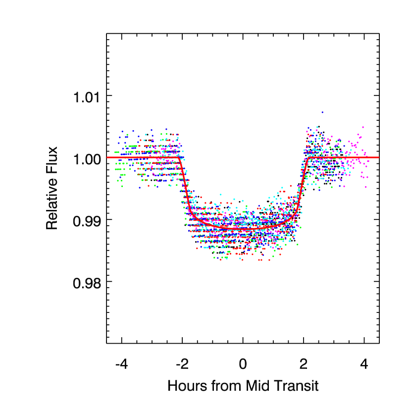
Figure 1: Phased light curve of HAT-P-33b transits with different colors representing different light curves. To revisit the system parameters, seven light curves were simultaneously fitted with the published RV observations (Figure 2) as described in §3, resulting in the best-fitting model shown by the solid red line.

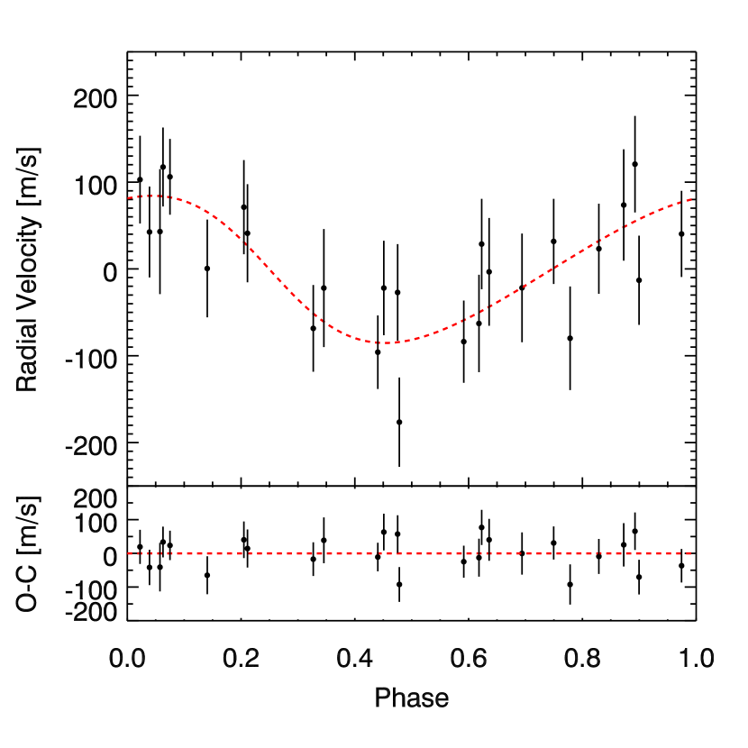
Figure 2: The radial velocity observations of HAT-P-33 from Knutson et al. (2014), jointly fitted with our photometric data (see Figure 1 and §3), resulting in the best-fitting keplerian orbit model shown by the dashed red line. The residuals from the best-fitting model with an RMS scatter of $47.5\,\rm{m\,s^{-1}}$ is shown at the bottom.

As expected, our RV parameters are consistent with those of Knutson et al. (2014), which resulted from the same RV datasets. These RV parameters also agree with the results from Hartman et al. (2011), though their RV datasets contains four fewer points. As with Knutson et al. (2014), we did not find long-period trend in the RV residuals, so we give the minimum mass of a potential planetary perturber following the convention defined by Wright et al. (2007).

The resulting transit parameters also agree with those from Hartman et al. (2011) except some with slight differences, including a lower impact parameter ($b$), a smaller value for the planet to star radius ratio ($R_{P}/R_{*}$), a shorter ingress/egress duration ($\tau$), a shorter total duration ($T_{14}$) and a larger Inclination ($i$). Comparing to the published work, which was based on only one full-transit light curve, our results are more robust, as a consequence of being based on the seven complete light curves.

Our stellar parameters show agreement with those of Hartman et al. (2011), which were chosen as the spectroscopic priors for the global fit in advance. And finally, the planetary parameters of HAT-P-33b calculated based on the derived RV, transit and stellar parameters also agree well with those in Hartman et al. (2011).

4.2 Mid-Transit Times

Figure 3: Seventeen transit light curves for HAT-P-33 obtained by Hartman et al. (2011) and this work, with which we can estimate the mid-transit times through the separate fits (see §3). The resulting best-fitting model for each light curve is shown by the solid red line, with residuals on the right. Both light curves and residuals are displaced vertically for clarity. For more details of our light curves, see Table 1.

In order to revisit the orbital ephemeris and seek TTV signals for the HAT-P-33b system, we acquired accurate mid-transit times ($T_{\rm c}$) through separately fitting each light curve. The best-fitting models are shown in Figure 3 and the resulting mid-transit times are listed in Table 4, with uncertainties obtained with the DE-MC method. We fitted obtained transit times with a linear function of transit epoch number ($N$),

Table 4: Mid-transit times for HAT-P-33b

Epoch	Telescope	$T_{\rm c}$	$\sigma_{T_{\rm c}}$	$O-C$
		(${\rm BJD_{TDB}}$)	(second)	(second)
-557	FLWO	2454099.85310	41.47	-192.40
-462	FLWO	2454429.93117	47.52	64.29
-427	FLWO	2454551.53949	50.11	211.56
-357	FLWO	2454794.75180	31.70	112.99
-355	FLWO	2454801.69988	63.94	56.88
-123	FLWO	2455607.77606	51.84	-112.18
-121	FLWO	2455614.72513	31.24	-101.77
173	Schmidt	2456636.22181	62.21	-5.85
196	$60\,{\rm cm}$	2456716.13465	59.62	-12.65
196	Schmidt	2456716.13498	56.16	15.86
198	$60\,{\rm cm}$	2456723.08352	40.15	-19.52
198	Schmidt	2456723.08417	50.52	36.64
289	Schmidt	2457039.26162	39.74	58.23
291	Schmidt	2457046.20981	39.74	-7.39
293	Schmidt	2457053.15793	40.61	-79.05
297	Schmidt	2457067.05749	37.15	64.46
392	$60\,{\rm cm}$	2457397.13183	57.02	-1.12

$$T_{\rm c}[N]=T_{\rm c}[0]+NP,$$ (1)

where $P$ is the planetary orbital period, $T_{\rm c}[0]$ represents the zero epoch. The best-fitting values are

$$T_{\rm c}[0]=2456035.137750\pm 0.000272\,[\rm{BJD_{TDB}}],$$ (2)

and

$$P=3.47447472\pm 0.00000088[{\rm days}].$$ (3)

Our orbital ephemeris agree well with the result from Hartman et al. (2011).

To get conservative uncertainty estimates for a more reliable future observation schedule, the uncertainties for the mid-transit times during the fitting were rescaled through a common factor to get $\chi^{2}/N_{\rm dof}=1$. However, the uncertainties of mid-transit times listed in Table 4 were not rescaled in this way, nor were the error bars plotted in Figure 4.

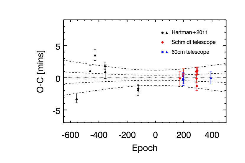
Figure 4: The points indicate the residuals of mid-transit times for HAT-P-33b from our linear orbital ephemeris (see eq.1-3), which is shown by the dotted line in the figure. The dashed lines indicate the propagation of $\pm 1\,\sigma$ and $\pm 3\,\sigma$ errors of the orbital ephemeris. We use different colors to distinguish the transits obtained by diverse groups or telescopes. The filled circles mark the full transits and the triangles represent the partial transits. As you can see, the black points are calculated from the published data (Hartman et al., 2011) which has only one full transit. The red and blue points are obtained from our photometric data, which have nine full transits and one partial transit.

Figure 4 displays the deviations of mid-transit times from the linear orbital ephemeris (eq.1-3), with an RMS of $93.68\,{\rm s}$. This value is largely affected by the mid-transit times derived from the published light curves, which gives an RMS of $144.12\,{\rm s}$ over a $4\,{\rm year}$ time span. As a contrast, the RMS of mid-transit times derived from our data is only $41.87\,{\rm s}$ within a time span of $3\,{\rm year}$. The large deviation of mid-transit times from the published light curves may be mainly caused by their incomplete coverages. In total, most of the mid-transit times are in the $\pm 3\,\sigma$ errors range of the orbital ephemeris. Especially for the mid-transit times resulted from our photometric data, which are very consistent with the $\pm 1\,\sigma$ errors.

4.3 Limits On Additional Perturbers

Although neither significant TTVs nor a residual RV signal were found, we can place the upper mass limits of a potential close-in perturbing planet in the HAT-P-33 system. The results are shown in Figure 5.

The host star (HAT-P-33) is an active late-F dwarf (Hartman et al., 2011), which has a large RV uncertainty (RMS=$47.5\,\rm{m\,s^{-1}}$). The mass limits based on the RV residuals following the convention in Wright et al. (2007) is thus very loose, as indicated by the black dashed line in Figure 5, which can only exclude a perturber with a mass larger than $0.6\,{\rm\,M_{\rm J}}$ near the 1:5 resonances (0.69-day orbit) or $2.0\,{\rm\,M_{\rm J}}$ near the 5:1 resonances (17.37-day orbit).

Fortunately, TTV measurements are less sensitive to the stellar activity than are Doppler measurements. We made use of the MERCURY6 orbit integration package Chambers (1999) to place upper mass limits of a potential perturbing body. The TTV data exhibited a RMS scatter of $93.68\,{\rm s}$.

In our simulations, we assumed that the orbits for both the known hot Jupiter and a potential perturber are coplanar and circular, which would gives the most conservative estimate of upper mass limits of the potential perturber (Bean, 2009; Fukui et al., 2011). The arguments of periastron, $\omega$, the ascending nodes, $\Omega$, and the initial mean anomalies, $M_{0}$, of the known hot Jupiter and a potential perturber are fixed to $\omega=88^{\circ}$ (from Table 3), $\Omega=270^{\circ}$, and $M_{0}=0^{\circ}$. We explored the mass space of the potential perturber for both interior and exterior orbits with the orbital period ratio from 1/5 to 5 times (0.69 to $17.37\,{\rm days}$) that of HAT-P-33b, which is equivalent to a semi-major axis range from 0.017 to $0.154\,{\rm AU}$. We incremented the perturber’s semi-major axis by $0.00001\,{\rm AU}$. The resolution is enough to depict the constraints on the perturber mass in the resonant configurations, that the TTV signals are significantly sensitive to (Agol & Steffen, 2007; Holman & Murray, 2005). In each increment of $a$, we obtained the upper mass limit of the potential perturber by iterative linear interpolation with an initial mass of $1.0\,{\rm M_{\oplus}}$ and a convergence tolerance of $1.0\,{\rm s}$ for the TTVs.

Comparing to the loose limits by RV data, the mass limits from our TTV measurements are much tighter near the low-order mean-motion resonances, as illustrated by the black solid line in Figure 5. We can exclude the existence of a perturber with mass larger than 0.6, 0.3, 0.5, 0.5, and $0.3\,{\rm M_{\oplus}}$ near the 1:3, 1:2, 2:3, 3:2, and 2:1 resonances, respectively.

In Figure 5, we also present the the dynamical stability in the hypothetical three-body system through Mean Exponential Growth of Nearby Orbits (MEGNO) Index (Goździewski et al., 2001; Cincotta et al., 2003; Hinse et al., 2010). The resulting dynamical stability map agrees well with that obtained by the analytic method described in Barnes & Greenberg (2006).

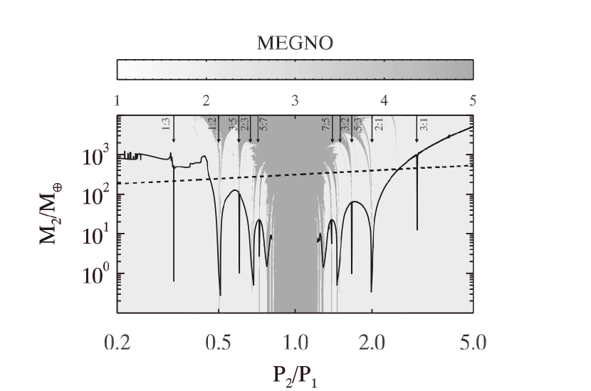
Figure 5: The upper mass limits on a potential additional perturber vs. the period ratio of the perturber ($P_{2}$) and HAT-P33b ($P_{1}$). The black dashed line shows the loose mass limits of a potential perturber based on the RV residuals (RMS=$47.5\,\rm{m\,s^{-1}}$), from which we can only rule out the existence of a perturber with mass comparable to Jupiter. However, the constraints from TTVs (RMS=$93.68\,\rm{s}$) are much tighter, especially near the the low-order mean-motion resonances (see the vertical arrows) that even a perturber with mass similar to Earth can been excluded. The color coding indicates overall system stability. For values larger than 5, the system is strongly chaotic and hence likely to be unstable. In general, chaotic regions are mainly because of two-body mean-motion resonances (indicated by vertical arrows). When the perturber is in the vicinity to the transiting planet then strong mutual interactions render the system to be unstable resulting in close-encounters or ejections of one or both planets.

5 SUMMARY AND CONCLUSIONS

We initiated the transiting exoplanet monitoring project (TEMP) to study the known exoplanets in great detail, with specific goals of obtaining a better grasp of planetary interior structures, formation and evolution.

One of the initial targets for TEMP, HAT-P-33b, has been observed by two telescopes from 2013 December to 2016 January. In total, we obtained ten light curves of eight different transit events, thereby substantially enriching the photometric database of HAT-P-33b.

To revisit the system parameters of HAT-P-33b, we have performed a global fit based on our new light curves and the expanded RV data (Knutson et al., 2014). Though most of the results agree well with those from the published work (Hartman et al., 2011; Knutson et al., 2014), some slight discrepancies still exist in the transit parameters.

We also separately conducted fits for the seventeen light curves to obtain precise mid-transit times. Along with these, we revisited the orbital ephemeris for HAT-P-33b, which agrees well with that in Hartman et al. (2011).

Though no substantial TTV signal has been found from the linear orbital ephemeris of HAT-P-33b, we can constrain the upper mass limits of a potential close-in perturbing planet based on the measured TTVs with an RMS scatter of $93.68\,\rm{s}$. The restriction is much stronger near the low-order mean-motion resonances. We can exclude the existence of a planet with mass larger than 0.6, 0.3, 0.5, 0.5, and $0.3\,{\rm M_{\oplus}}$ near the 1:3, 1:2, 2:3, 3:2, and 2:1 resonances, respectively. However, we still cannot rule out the existence of additional close-in planets in the non-resonant area. Whether additional planets frequently exist in the nearby non-resonant area of hot Jupiters is an open question. Further work is needed to answer this question, and hence to better reveal the nature of planetary formation and evolution.

References

- Agol & Steffen (2007) Agol, E., & Steffen, J. H. 2007, MNRAS, 374, 941
- Barnes & Greenberg (2006) Barnes, R., & Greenberg, R. 2006, ApJ, 647, L163
- Batygin et al. (2016) Batygin, K., Bodenheimer, P. H., & Laughlin, G. P. 2016, ApJ, 829, 114
- Bean (2009) Bean, J. L. 2009, A&A, 506, 369
- Becker et al. (2015) Becker, J. C., Vanderburg, A., Adams, F. C., Rappaport, S. A., & Schwengeler, H. M. 2015, ApJ, 812, L18
- Bertin & Arnouts (1996) Bertin, E., & Arnouts, S. 1996, A&AS, 117, 393
- Bodenheimer et al. (2000) Bodenheimer, P., Hubickyj, O., & Lissauer, J. J. 2000, Icarus, 143, 2
- Chambers (1999) Chambers, J. E. 1999, MNRAS, 304, 793
- Cincotta et al. (2003) Cincotta, P. M., Giordano, C. M., & Simó, C. 2003, Physica D Nonlinear Phenomena, 182, 151
- Claret & Bloemen (2011) Claret, A., & Bloemen, S. 2011, A&A, 529, A75
- Collins et al. (2017) Collins, K. A., Kielkopf, J. F., & Stassun, K. G. 2017, AJ, 153, 78
- Eastman et al. (2010) Eastman, J., Siverd, R., & Gaudi, B. S. 2010, PASP, 122, 935
- Eastman et al. (2013) Eastman, J., Gaudi, B. S., & Agol, E. 2013, PASP, 125, 83
- Fabrycky et al. (2014) Fabrycky, D. C., Lissauer, J. J., Ragozzine, D., et al. 2014, ApJ, 790, 146
- Ford & Rasio (2008) Ford, E. B., & Rasio, F. A. 2008, ApJ, 686, 621
- Fukui et al. (2011) Fukui, A., Narita, N., Tristram, P. J., et al. 2011, PASJ, 63, 287
- Fukui et al. (2013) Fukui, A., Narita, N., Kurosaki, K., et al. 2013, ApJ, 770, 95
- Goździewski et al. (2001) Goździewski, K., Bois, E., Maciejewski, A. J., & Kiseleva-Eggleton, L. 2001, A&A, 378, 569
- Hadden & Lithwick (2015) Hadden, S., & Lithwick, Y. 2015, AAS/Division for Extreme Solar Systems Abstracts, 3, 102.06
- Hartman et al. (2011) Hartman, J. D., Bakos, G. Á., Torres, G., et al. 2011, ApJ, 742, 59
- Hinse et al. (2010) Hinse, T. C., Christou, A. A., Alvarellos, J. L. A., & Goździewski, K. 2010, MNRAS, 404, 837
- Hinse et al. (2015) Hinse, T. C., Han, W., Yoon, J.-N., et al. 2015, Journal of Astronomy and Space Sciences, 32, 21
- Holman & Murray (2005) Holman, M. J., & Murray, N. W. 2005, Science, 307, 1288
- Howell et al. (2014) Howell, S. B., Sobeck, C., Haas, M., et al. 2014, PASP, 126, 398
- Knutson et al. (2014) Knutson, H. A., Fulton, B. J., Montet, B. T., et al. 2014, ApJ, 785, 126
- Lendl et al. (2013) Lendl, M., Delrez, L., Gillon, M., Jehin, E., & Queloz, D. 2013, Protostars and Planets VI Posters, 2
- Lin et al. (1996) Lin, D. N. C., Bodenheimer, P., & Richardson, D. C. 1996, Nature, 380, 606
- Lithwick et al. (2012) Lithwick, Y., Xie, J., & Wu, Y. 2012, ApJ, 761, 122
- Mancini et al. (2013) Mancini, L., Ciceri, S., Chen, G., et al. 2013, MNRAS, 436, 2
- Mancini et al. (2016) Mancini, L., Giordano, M., Mollière, P., et al. 2016, MNRAS, 461, 1053
- Nagasawa et al. (2008) Nagasawa, M., Ida, S., & Bessho, T. 2008, ApJ, 678, 498
- Nutzman et al. (2011) Nutzman, P. A., Fabrycky, D. C., & Fortney, J. J. 2011, ApJ, 740, L10
- Ricker et al. (2015) Ricker, G. R., Winn, J. N., Vanderspek, R., et al. 2015, Journal of Astronomical Telescopes, Instruments, and Systems, 1, 014003
- Sanchis-Ojeda & Winn (2011) Sanchis-Ojeda, R., & Winn, J. N. 2011, ApJ, 743, 61
- Sanchis-Ojeda et al. (2013) Sanchis-Ojeda, R., Winn, J. N., & Fabrycky, D. C. 2013, Astronomische Nachrichten, 334, 180
- Sato et al. (2005) Sato, B., Fischer, D. A., Henry, G. W., et al. 2005, ApJ, 633, 465
- Seeliger et al. (2015) Seeliger, M., Kitze, M., Errmann, R., et al. 2015, MNRAS, 451, 4060
- Sing et al. (2016) Sing, D. K., Fortney, J. J., Nikolov, N., et al. 2016, Nature, 529, 59
- Southworth et al. (2009) Southworth, J., Hinse, T. C., Jørgensen, U. G., et al. 2009, MNRAS, 396, 1023
- Star Cartier et al. (2016) Star Cartier, K. M., Zhao, M., Wright, J., & Beatty, T. G. 2016, American Astronomical Society Meeting Abstracts, 227, 306.06
- Torres et al. (2010) Torres, G., Andersen, J., & Giménez, A. 2010, A&A Rev., 18, 67
- Wang et al. (2016) Wang, S.-H., Wang, Y.-H., & Zang, X.-J. 2016, AJ, submitted
- Wright et al. (2007) Wright, J. T., Marcy, G. W., Fischer, D. A., et al. 2007, ApJ, 657, 533
- Wu & Murray (2003) Wu, Y., & Murray, N. 2003, ApJ, 589, 605
- Wu & Lithwick (2011) Wu, Y., & Lithwick, Y. 2011, ApJ, 735, 109
- Xie et al. (2014) Xie, J.-W., Wu, Y., & Lithwick, Y. 2014, ApJ, 789, 165
- Zhou et al. (1999) Zhou, X., Chen, J., Xu, W., et al. 1999, PASP, 111, 909
- Zhou et al. (2001) Zhou, X., Jiang, Z.-J., Xue, S.-J., et al. 2001, Chinese J. Astron. Astrophys., 1, 372