Invariant-based pulse design for three-level systems without the rotating-wave approximation

Abstract

In this paper, a scheme is put forward to design pulses which drive a three-level system based on the reverse engineering with Lewis-Riesenfeld invariant theory. The scheme can be applied to a three-level system even when the rotating-wave approximation (RWA) can not be used. The amplitudes of pulses and the maximal values of detunings in the system could be easily controlled by adjusting control parameters. We analyze the dynamics of the system by an invariant operator, so additional couplings are unnecessary. Moreover, the approaches to avoid singularity of pulses are studied and several useful results are obtained. We hope the scheme could contribute to fast quantum information processing without RWA.

I INTRODUCTION

Manipulating physical systems with time-dependent electromagnetic fields, which is important for high-precision quantum information processing, has attracted growing interests in recent years. The adiabatic passage FewellAJP50 ; BergmannRMP70 ; VitanovARPC52 ; KralRMP79 is one of typical methods to design and control time-dependent pulses, which has been widely used in numerous previous schemes ZhengPRL95 ; YangPRL92 ; MolerPRA75 ; DengPRA74 . The adiabatic passage is approved for its robustness against the fluctuations of control parameters, while it is also criticized for the low speed caused by the limit of adiabatic condition. To accelerate evolutions of physical systems, many methods DemirplakJPCA107 ; BerryJPA42 ; ChenPRL105 ; CampoPRL111 ; CampoPRL109 ; CampoPRA84 ; CampoEPL96 ; CampoSR2 ; DeffnerPRX4 ; ChenPRA82 ; ChenPRA83 ; ChenPRA84 ; MugaJPB42 ; MugaJPB43 ; ChenPRL104 have been proposed. Since they are related to the adiabatic passage, but provide alternative paths without the adiabatic condition for evolutions of physical systems, these methods DemirplakJPCA107 ; BerryJPA42 ; ChenPRL105 ; CampoPRL111 ; CampoPRL109 ; CampoPRA84 ; CampoEPL96 ; CampoSR2 ; DeffnerPRX4 ; ChenPRA82 ; ChenPRA83 ; ChenPRA84 ; MugaJPB42 ; MugaJPB43 ; ChenPRL104 are arranged as a new kind of technique named by shortcuts to adiabaticity (STA). In the past several years, STA has drawn much attention of researchers, and has subsequently been used in many physical systems, such as superconducting systems KangPRA94 ; ZhangSR5 , atom-cavity systems ChenPRA86 ; yehongPRA89 , and spin-NV center systems SongPRA93 ; SongNJP18 . Besides, many schemes IbanezPRL109 ; IbanezPRA87 ; IbanezPRA89 ; yehongPRA93 ; TorronteguiPRA89 ; GaraotPRA89 ; qichengOE24 ; KangSR6 have been put forward to improve or extend STA. Until now, STA could be used to design pulses perfectly in many different cases.

The previous schemes DemirplakJPCA107 ; BerryJPA42 ; ChenPRL105 ; CampoPRL111 ; CampoPRL109 ; CampoPRA84 ; CampoEPL96 ; CampoSR2 ; DeffnerPRX4 ; ChenPRA82 ; ChenPRA83 ; ChenPRA84 ; MugaJPB42 ; MugaJPB43 ; ChenPRL104 ; KangPRA94 ; ZhangSR5 ; ChenPRA86 ; yehongPRA89 ; SongPRA93 ; SongNJP18 ; IbanezPRL109 ; IbanezPRA87 ; IbanezPRA89 ; yehongPRA93 ; TorronteguiPRA89 ; GaraotPRA89 ; qichengOE24 ; KangSR6 with STA focused on the physical systems under the rotating-wave approximation (RWA). However, many recent schemes about superconducting systems SornborgerPRA70 ; LiuPRA90 ; SankPRL117 , optomechanical systems MalzPRA94 , semiconducting systems SongPRA94 , Bose-Einstein condensates HofferberthPRA76 , and NV centers ScheuerNJP16 have shown that, RWA may be invalid in the cases of ultra-fast operations and ultra-strong couplings. For example, Liu et al. LiuPRA90 have shown that RWA is broken down in the ultra-strong coupling, where the frequencies of pulses take the value of $10\times 2\pi$GHz and the coupling strengthes take the value of $1.021\times 2\pi$GHz. Moreover, Scheuer et al. ScheuerNJP16 have demonstrated in a NV center that, when using a magnetic field with a frequency of 30MHz, RWA can not be used for a qubit control if the Rabi frequency larger than 15MHz. From these examples SornborgerPRA70 ; LiuPRA90 ; SankPRL117 ; MalzPRA94 ; SongPRA94 ; HofferberthPRA76 ; ScheuerNJP16 , RWA may be invalid in fast quantum information processing, thus the applications of previous schemes DemirplakJPCA107 ; BerryJPA42 ; ChenPRL105 ; CampoPRL111 ; CampoPRL109 ; CampoPRA84 ; CampoEPL96 ; CampoSR2 ; DeffnerPRX4 ; ChenPRA82 ; ChenPRA83 ; ChenPRA84 ; MugaJPB42 ; MugaJPB43 ; ChenPRL104 ; KangPRA94 ; ZhangSR5 ; ChenPRA86 ; yehongPRA89 ; SongPRA93 ; SongNJP18 ; IbanezPRL109 ; IbanezPRA87 ; IbanezPRA89 ; yehongPRA93 ; TorronteguiPRA89 ; GaraotPRA89 ; qichengOE24 ; KangSR6 with STA would be limited. Therefore, it is worthwhile to study STA without RWA so that pulse design for fast quantum information processing could be more effective.

Last year, two schemes IbanezPRA92 ; ChenPRA91 have been proposed, which are about STA without RWA. One scheme ChenPRA91 is proposed by Chen et al., in which transitionless quantum driving (the counterdiabatic driving) is exploited to investigate the dynamics of both two- and three-level systems. It has shown that population transfers in both two- and three-level systems could be achieved in theory. The scheme ChenPRA91 is interesting, but it has a few disadvantages. First, using the transitionless quantum driving requires an extra coupling between the initial state and the final state, which may be hard to be realized in several cases. Besides, the control parameters are not flexible enough to control the amplitudes of pulses and maximal values of detunings. Moreover, how to reduce oscillations and avoid the singularity of pulses, which are two questions required to be considered when RWA is broken down, have not been discussed. The other interesting scheme IbanezPRA92 is proposed by Ibáñez et al., which is about pulse design for a two-level system with both transitionless quantum driving and invariant-based method with Lewis-Riesenfeld theory LewisJMP10 . Their scheme IbanezPRA92 has shown many interesting results. For example, using invariant-based method does not require any extra couplings, which makes the pulse design more feasible in experiments. Moreover, the singularity of pulses can be avoided by choosing control parameters suitably. Furthermore, they have shown that an invariant-based pulse design can help to achieve a population transfer in a two-level system with a perfect fidelity. These interesting results have demonstrated that the invariant-based method is very promising. However, different systems possess different dynamic features. Invariants for a two-level system without RWA can not properly describe the dynamics of a three-level system without RWA. Moreover, with the dimensions increase, the complexity of invariants would greatly increase. Therefore, the scheme IbanezPRA92 can not be directly applied to a three-level system without RWA. But three-level systems are very important in quantum information processing, as many quantum information tasks can be implemented in physical systems which are equivalent or approximately equivalent to three-level systems lumeiPRA89 ; yehongPRA91 ; LonghiLPR3 ; LonghiJPB44 ; OrnigottiJPB41 ; RangelovPRA85 . So it is necessary to research dynamics of three-level systems without RWA. Considering the advantages of the invariant-based method, if it can be applied to pulse design for three-level systems without RWA, we can realize many interesting quantum information tasks with ultra-fast operations and ultra-strong couplings. That requires us firstly to find out an invariant for three-level systems without RWA.

In this paper, inspired by the schemes IbanezPRA92 ; ChenPRA91 , we propose a scheme to design pulses for a three-level system without RWA. The scheme is based on a new-found invariant operator, which can help to study the dynamics of a three-level system without RWA. The scheme has some advantages, such as high speed, robustness against fluctuations of parameters, no requirements on extra couplings, etc.. These advantages would be clearly shown in the following sections.

The article is organized as follows. In Sec. II, we briefly review the Lewis-Riesenfeld invariant theory. In Sec. III, we give an invariant for a three-level system without RWA. Based on this invariant, the mathematical expressions of pulses and detunings are determined. In Sec. IV, we complete population transfers for a three-level system without RWA as examples to show the validity of the scheme. Finally, the conclusions are given in Sec. V.

II Lewis-Riesenfeld invariant theory

In this section, let us briefly introduce Lewis-Riesenfeld theory LewisJMP10 . We consider a quantum system which has a time-dependent Hamiltonian $H(t)$. Now, we introduce an invariant Hermitian operator $I(t)$, which satisfies ($\hbar=1$)

$$i\frac{\partial}{\partial t}I(t)-[H(t),I(t)]=0.$$ (1)

If $|\psi(t)\rangle$ is a solution of the time-dependent Schrödinger equation $i\partial_{t}|\psi(t)\rangle=H(t)|\psi(t)\rangle$, $I(t)|\psi(t)\rangle$ is a solution as well. Moreover, $|\psi(t)\rangle$ can be expanded by eigenvectors of $I(t)$ as

$$|\psi(t)\rangle=\sum\limits_{k}C_{k}e^{i\theta_{k}}|\phi_{k}(t)\rangle,$$ (2)

where, $|\phi_{k}(t)\rangle$ is the $k$th eigenvector of $I(t)$, and $C_{k}=\langle\phi_{k}(0)|\psi(0)\rangle$ is the corresponding coefficient. $\theta_{k}$ is the Lewis-Riesenfeld phase for $|\phi_{k}(t)\rangle$, which satisfies

$$\dot{\theta}_{k}=\langle\phi_{k}(t)|i\partial_{t}-H(t)|\phi_{k}(t)\rangle,$$ (3)

with $\theta_{k}(t_{i})=0$ ($t_{i}$ is the initial time).

III Invariant-based pulse design for three-level systems without the rotating-wave approximation

Let us start with a three-level system with two ground states $|1\rangle$, $|3\rangle$, and an excited state $|2\rangle$ shown in Fig. 1.

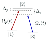
Figure 1: The energy levels of the three-level system.

Without RWA, the Hamiltonian of this system can be written by

$$H(t)=\left[\begin{array}[]{ccc}-\omega_{p}-\Delta_{p}(t)&\ \Omega_{p}(t)\cos(\omega_{p}t)&\ 0\\ \Omega_{p}^{*}(t)\cos(\omega_{p}t)&\ 0&\ \Omega_{s}^{*}(t)\cos(\omega_{s}t)\\ 0&\ \Omega_{s}(t)\cos(\omega_{s}t)&\ -\omega_{s}-\Delta_{s}(t)\\ \end{array}\right],$$ (7)

in basis $\{|1\rangle,|2\rangle,|3\rangle\}$, where, $\Omega_{p}(t)$, $\Omega_{s}(t)$ are the pump and Stokes pulses driving the transitions $|1\rangle\leftrightarrow|2\rangle$ and $|3\rangle\leftrightarrow|2\rangle$, respectively. $\Omega_{p}^{*}(t)$, $\Omega_{s}^{*}(t)$ are the complex conjugates of $\Omega_{p}(t)$, $\Omega_{s}(t)$, respectively. $\omega_{p}$ and $\omega_{s}$ are the frequencies of pump and Stokes pulses, respectively. $\Delta_{p}(t)$ and $\Delta_{s}(t)$ denote the detunings of the pump and Stokes pulses from their relevant transitions, respectively. By analyzing Eqs. (1) and (7) with some undetermined coefficients, we find out a Lewis-Riesenfeld invariant as follows:

$$I(t)=\left[\begin{array}[]{ccc}I_{11}&\ I_{12}&\ I_{13}\\ I_{12}^{*}&\ I_{22}&\ I_{23}\\ I_{13}^{*}&\ I_{23}^{*}&\ I_{33}\\ \end{array}\right],$$ (11)

and the matrix elements of $I(t)$ are given as

$$I_{11} =\cos 2\lambda(\cos^{2}\alpha\cos^{2}\beta-\sin^{2}\alpha)$$ (14)

$$+\cos\epsilon\cos\beta\sin 2\alpha\sin 2\lambda,$$

$$I_{12} =(\cos\alpha\cos 2\lambda\cos\beta+e^{-i\epsilon}\sin\alpha\sin 2\lambda)\sin\beta,$$ (16)

$$I_{13} =\frac{1}{4}\cos 2\lambda(3+\cos 2\beta)\sin 2\alpha$$ (20)

$$-\cos\beta(\cos\epsilon\cos 2\alpha+i\sin\epsilon)\sin 2\lambda,$$

$$I_{22} =\cos 2\lambda\sin^{2}\beta,$$ (22)

$$I_{23} =(\sin\alpha\cos 2\lambda\cos\beta-e^{i\epsilon}\cos\alpha\sin 2\lambda)\sin\beta,$$ (24)

$$I_{33} =\cos 2\lambda(\sin^{2}\alpha\cos^{2}\beta-\cos^{2}\alpha)$$ (28)

$$-\cos\epsilon\cos\beta\sin 2\alpha\sin 2\lambda.$$

In Eq. (14), $\alpha$, $\beta$, $\epsilon$, $\lambda$ are four auxiliary time-dependent parameters, and they are required to satisfy

$$\dot{\alpha}=\dot{\lambda}\cos\beta\cos\epsilon.$$ (29)

The invariant $I(t)$ has three eigenvectors as follows:

$$|\phi_{+}(t)\rangle=\left[\begin{array}[]{c}\cos\alpha\cos\beta\cos\lambda+e^{i\epsilon}\sin\alpha\sin\lambda\\ \sin\beta\cos\lambda\\ \sin\alpha\cos\beta\cos\lambda-e^{i\epsilon}\cos\alpha\sin\lambda\\ \end{array}\right],$$ (33)

(34)

$$|\phi_{-}(t)\rangle=\left[\begin{array}[]{c}\cos\alpha\cos\beta\sin\lambda-e^{i\epsilon}\sin\alpha\cos\lambda\\ \sin\beta\sin\lambda\\ \sin\alpha\cos\beta\sin\lambda+e^{i\epsilon}\cos\alpha\cos\lambda\\ \end{array}\right],$$ (38)

(39)

$$|\phi_{0}(t)\rangle=\left[\begin{array}[]{c}\cos\alpha\sin\beta\\ -\cos\beta\\ \sin\alpha\sin\beta\\ \end{array}\right],$$ (43)

which corresponds to eigenvalues 1, -1 and 0 of $I(t)$.

Solving Eq. (1) with $H(t)$ in Eq. (7) and $I(t)$ in Eq. (11), we obtain the following results

$$\Omega_{p}(t)\cos(\omega_{p}t) =i\dot{\lambda}e^{-i\epsilon}\sin\alpha\sin\beta$$ (46)

$$+\frac{1}{2}\cos\alpha(-2i\dot{\beta}+\dot{\theta}\sin 2\beta),$$

$$\Omega_{s}(t)\cos(\omega_{s}t) =-i\dot{\lambda}e^{-i\epsilon}\cos\alpha\sin\beta$$ (50)

$$+\frac{1}{2}\sin\alpha(-2i\dot{\beta}+\dot{\theta}\sin 2\beta),$$

$$\omega_{p}+\Delta_{p}(t) =-\dot{\epsilon}\sin^{2}\alpha+\dot{\theta}(\cos^{2}\alpha\sin^{2}\beta-\cos^{2}\beta)$$ (54)

$$-\dot{\lambda}\sin\epsilon\sin 2\alpha\cos\beta,$$

$$\omega_{s}+\Delta_{s}(t) =-\dot{\epsilon}\cos^{2}\alpha+\dot{\theta}(\sin^{2}\alpha\sin^{2}\beta-\cos^{2}\beta)$$ (58)

$$+\dot{\lambda}\sin\epsilon\sin 2\alpha\cos\beta.$$

In Eq (46), $\theta$ is the Lewis-Riesenfeld phase of $|\phi_{0}(t)\rangle$, which could be solved by

$$\dot{\theta}=\langle\phi_{0}(t)|i\partial_{t}-H(t)|\phi_{0}(t)\rangle=-\frac{\dot{\epsilon}+2\dot{\lambda}\sin\epsilon\cos\beta\cot 2\alpha}{\sin^{2}\beta}.$$ (59)

Besides, the Lewis-Riesenfeld phases of $|\phi_{+}(t)\rangle$ and $|\phi_{-}(t)\rangle$ are both zero.

With the results above, we can use the following formula to calculate the evolution of the system

$$|\psi(t)\rangle =(\langle\phi_{+}(0)|\psi(0)\rangle)|\phi_{+}(t)\rangle+(\langle\phi_{-}(0)|\psi(0)\rangle)|\phi_{-}(t)\rangle$$ (62)

$$+e^{i\theta}(\langle\phi_{0}(0)|\psi(0)\rangle)|\phi_{0}(t)\rangle.$$

IV Population transfers for a three-level system

Using the results shown in Sec. III, we would like to perform population transfers for a three-level system to check the validity of the scheme. For simplicity, the condition $\dot{\lambda}=\dot{\alpha}=0$ is set, so $\dot{\epsilon}=-\dot{\theta}\sin^{2}\beta$ can be obtained from Eq. (59), and Eq. (46) reduces to

$$\Omega_{p}(t)\cos(\omega_{p}t) =\frac{1}{2}\cos\alpha(-2i\dot{\beta}+\dot{\theta}\sin 2\beta),$$ (63)

$$\Omega_{s}(t)\cos(\omega_{s}t) =\frac{1}{2}\sin\alpha(-2i\dot{\beta}+\dot{\theta}\sin 2\beta),$$ (65)

$$\omega_{p}+\Delta_{p}(t) =-\dot{\theta}\cos 2\beta,$$ (67)

$$\omega_{s}+\Delta_{s}(t) =-\dot{\theta}\cos 2\beta.$$ (69)

Then, two time-independent coefficients $\kappa_{p}$ and $\kappa_{s}$ are introduced, such that

$$\omega_{p}+\Delta_{p}(t) =-\kappa_{p}\dot{\theta}+(\kappa_{p}-\cos 2\beta)\dot{\theta},$$ (70)

$$\omega_{s}+\Delta_{s}(t) =-\kappa_{s}\dot{\theta}+(\kappa_{s}-\cos 2\beta)\dot{\theta}.$$ (72)

In addition, we introduce a positive time-independent parameter $\omega$, which has the scale of frequency. Assuming $\dot{\theta}=-\omega$, Eq. (70) can be replaced by

$$\omega_{p}+\Delta_{p}(t) =\kappa_{p}\omega-(\kappa_{p}-\cos 2\beta)\omega,$$ (73)

$$\omega_{s}+\Delta_{s}(t) =\kappa_{s}\omega-(\kappa_{s}-\cos 2\beta)\omega.$$ (75)

Furthermore, Eq. (73) can be rewritten by

$$\omega_{p} =\kappa_{p}\omega,$$ (76)

$$\omega_{s} =\kappa_{s}\omega,$$ (78)

$$\Delta_{p}(t) =-(\kappa_{p}-\cos 2\beta)\omega,$$ (80)

$$\Delta_{s}(t) =-(\kappa_{s}-\cos 2\beta)\omega.$$ (82)

For a brief discussion, we consider that the pump and Stokes pulses have the same frequency $\omega_{p}=\omega_{s}$, but different polarization directions. Besides, the two-photon resonance condition, where $\Delta_{p}(t)=\Delta_{s}(t)=\Delta(t)$, is considered. With assumptions shown above, a simple choice is to set $\kappa_{p}=\kappa_{s}=1$, such that

$$\omega_{p}=\omega_{s} =\omega,$$ (83)

$$\Delta(t) =-2\omega\sin^{2}\beta,$$ (85)

$$\Omega_{p}(t)\cos(\omega t) =-\frac{\cos\alpha}{2}(2i\dot{\beta}+\omega\sin 2\beta),$$ (87)

$$\Omega_{s}(t)\cos(\omega t) =-\frac{\sin\alpha}{2}(2i\dot{\beta}+\omega\sin 2\beta).$$ (89)

In the following, we design the parameters from different viewpoints and analyze the physical feasibility of the population transfers.

IV.1 Pulse design with smooth functions

We suppose that a population transfer starts at $t=0$ and ends at $t=T$. And the initial state of the system is $|\psi(0)\rangle=|1\rangle$. Considering the following requirements:

(i) The pump and Stokes pulses could be smoothly turned on and turned off.

(ii) To avoid the singularity of the pump and Rabi frequencies of Stokes pulses.

(iii) To avoid overlarge detunings or pulses.

$\beta$ and its time derivative $\dot{\beta}$ can be designed as follows:

$$\beta =\frac{A}{2}[1-\cos(\frac{2\pi t}{T})]\cos^{2}(\omega t),$$ (90)

$$\dot{\beta} =\frac{\pi A}{T}\sin(\frac{2\pi t}{T})\cos^{2}(\omega t)$$ (94)

$$-\frac{A\omega}{2}[1-\cos(\frac{2\pi t}{T})]\sin(2\omega t),$$

where $A$ is a time-independent coefficient controlling the maximal value of $\beta$. From Eq. (90), we have

$$\beta(0)=\beta(T)=\dot{\beta}(0)=\dot{\beta}(T)=0,$$ (95)

so the pump and Stokes pulses could be smoothly turned on and turned off. Moreover, when $A$ is not too large, the maximal values of detunings and amplitudes of pulses could be controlled in desired ranges. Besides, substituting Eq. (90) into Eq. (83), one can find that when $\cos(\omega t)\rightarrow 0$, we have $\sin 2\beta/\cos(\omega t)\rightarrow 0$ and $\dot{\beta}/\cos(\omega t)\rightarrow\mathrm{Const}$. Therefore, the singularity of Rabi frequencies of the pump and Stokes pulses can be eliminated.

On the other hand, using Eqs. (62) and (95), the final state of the system can be obtained

$$|\psi(T)\rangle=\left[\begin{array}[]{c}\cos^{2}\alpha+e^{i\epsilon}\sin^{2}\alpha\\ 0\\ (1-e^{i\epsilon})\sin\alpha\cos\alpha\\ \end{array}\right].$$ (99)

By choosing $\alpha=\pi/4$, we have $|\psi(T)\rangle=|3\rangle$ when

$$\epsilon(T)=\omega\int_{0}^{T}\sin^{2}\beta dt=\pi.$$ (100)

Solving Eq. (100) with numerical methods, some samples of the relations between $A$ and $\omega T$ are given in Table I.

Table I. $A$ with corresponding $\omega T$.            $A$                          $\omega T$            $0.2$                         $179.04\pi$            $0.3$                         $80.28\pi$            $0.4$                         $45.72\pi$            $0.5$                         $29.73\pi$            $0.6$                         $21.05\pi$            $0.7$                         $15.83\pi$

When $A=0.2$ ($A=0.3$), a population transfer would go through about 90 (40) pulse periods, which makes the Rabi frequencies of pump and Stokes pulses oscillate very quickly. Therefore, we focus on the cases when $A=0.4,0.5,0.6,0.7$ in the following. We define the population of state $|j\rangle$ as $P_{j}(t)=|\langle j|\psi(t)\rangle|^{2}$ ($j=1,2,3$). In addition, since $\alpha=\pi/4$ is chosen, we have $\Omega_{s}(t)=\Omega_{p}(t)=\Omega(t)$. The populations $P_{1}$, $P_{2}$, and $P_{3}$ versus $t/T$ with different parameters are shown in Fig. 2. Besides, the real (imaginary) part $\mathrm{Re}[\Omega(t)]$ ($\mathrm{Im}[\Omega(t)]$) of $\Omega(t)$ and the detuning $\Delta(t)$ versus $t/T$ with different parameters are shown in Fig. 3.

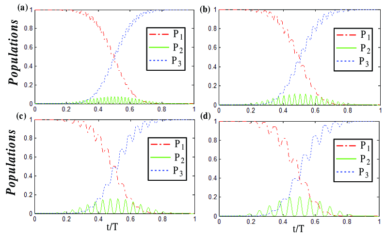
Figure 2: Populations $P_{1}$ (the dashed-dotted red line), $P_{2}$ (the solid green line), and $P_{3}$ (the dotted blue) versus $t/T$ with different parameters: (a) $A=0.4$, $\omega=45.7220\pi/T$; (b) $A=0.5$, $\omega=29.7323\pi/T$; (c) $A=0.6$, $\omega=21.0533\pi/T$; (d) $A=0.7$, $\omega=15.8274\pi/T$.

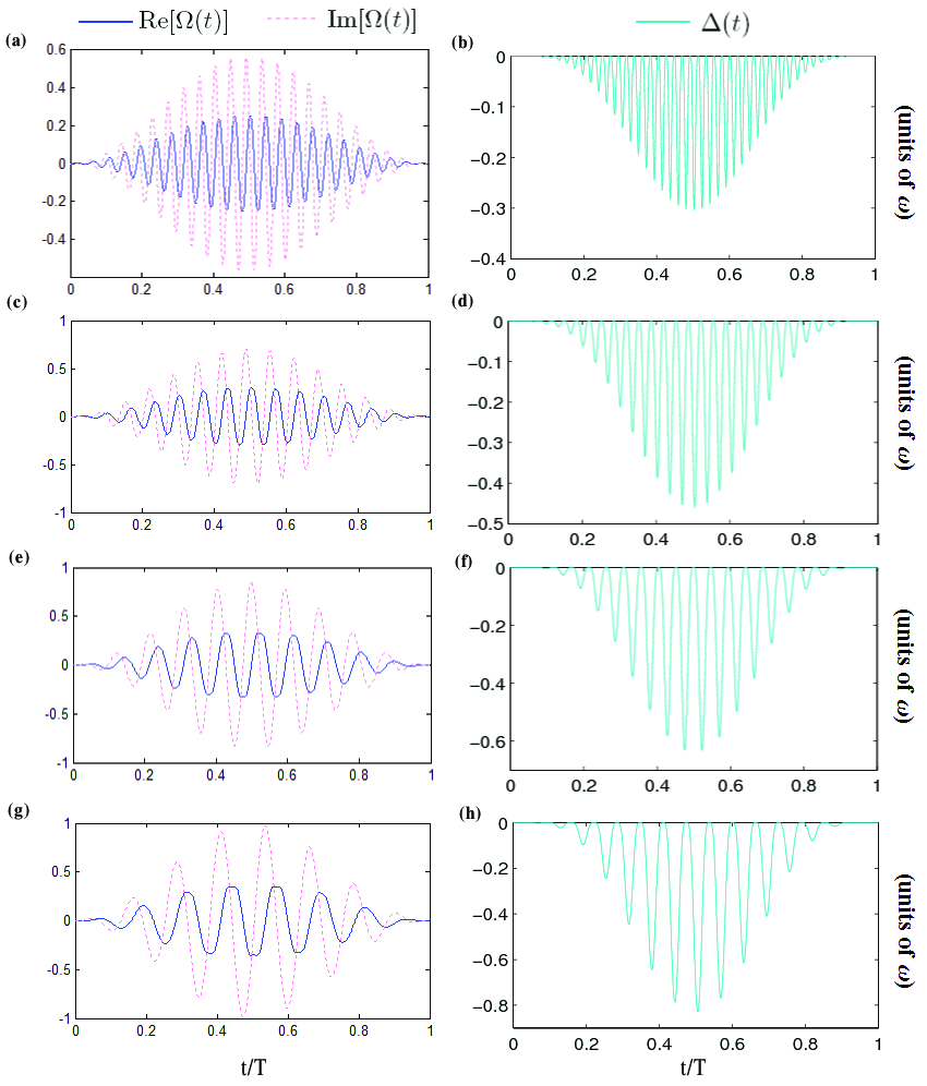
Figure 3: The real part $\mathrm{Re}[\Omega(t)]$ (the solid blue line) and the imaginary part $\mathrm{Im}[\Omega(t)]$ (the dotted pink line) of $\Omega(t)$, and the detuning $\Delta(t)$ (the light blue line) versus $t/T$ with different parameters: (a)-(b) $A=0.4$, $\omega=45.7220\pi/T$; (c)-(d) $A=0.5$, $\omega=29.7323\pi/T$; (e)-(f) $A=0.6$, $\omega=21.0533\pi/T$; (g)-(h) $A=0.7$, $\omega=15.8274\pi/T$.

According to Fig. 2, population transfers could be achieved with $A=0.4,0.5,0.6,0.7$. This proves the invariant given in Eq. (11) is correct, and the parameters designed in this section are valid. Moreover, it is easy to find out that the maximal population of the intermediate state $|2\rangle$ increases slightly when $A$ increases.

According to Fig. 3, the oscillations of pulses reduce when $A$ increases, since $A$ with larger value make the evolution of the system go through fewer pulse periods (as shown in Table I). When detunings and Rabi frequencies have too many oscillations, they may be difficult to be realized in experiments. To reduce the oscillations, one may increase $A$. However, from Fig. 3, the maximal values of ratios $\Omega(t)/\omega$ and $\Delta(t)/\omega$ increase when $A$ increases. When $A$ is too large, the pulses and detunings may go beyond the acceptable ranges. Therefore, when designing pulses with smooth functions for a real experiment, one should choose a suitable $A$ to make the pulses and detunings in acceptable ranges.

IV.2 Pulse design with modifications around singular points

In this part, we try to reduce the oscillations by choosing a flat varying $\beta$. And we try to avoid the singularity of pulses by modifying the pulses around their singular points. The modifications are based on the fact that the Cauchy principal value of

$$\int_{x_{0}-\varsigma}^{x_{0}+\varsigma}\frac{1}{\cos x}dx$$ (101)

is zero, where $x_{0}$ denotes a singular point of function $1/\cos x$, and $\varsigma$ is an arbitrary small value. Therefore, populations vary little in the time intervals around the singular points of $1/\cos(\omega t)$. We can make some modifications of pulses around the singular points of $1/\cos(\omega t)$.

Suppose that a population transfer starts at $t=0$ and ends at $t=T$, and the initial state of the system is $|\psi(0)\rangle=|1\rangle$. We maintain the condition $\alpha=\pi/4$ in this section. Instead of $\beta$ and $\dot{\beta}$ shown in part A, we choose $\bar{\beta}$ and $\dot{\bar{\beta}}$, respectively, as follows:

$$\bar{\beta} =\frac{B}{2}[1-\cos(\frac{2\pi t}{T})],$$ (102)

$$\dot{\bar{\beta}} =\frac{\pi B}{T}\sin(\frac{2\pi t}{T}),$$ (104)

where, $B$ is a time-independent coefficient controlling the maximal value of $\bar{\beta}$. In this case, pulses could still be smoothly turned on and turned off. But different from the $\beta$ and $\dot{\beta}$ designed in part A, the parameters that we chose here could not eliminate the singularity of pulses. However, when $B=A$, we have

$$\bar{\epsilon}(T)=\omega\int_{0}^{T}\sin^{2}\bar{\beta}dt\geq\omega\int_{0}^{T}\sin^{2}\beta dt=\epsilon(T).$$ (105)

So in the case of $B=A$, the maximal value of $\beta$ is approximately equal to that of $\bar{\beta}$, but the population transfer could be completed faster as it goes through fewer pulse periods. That means the oscillations of pulses decrease a lot compared with the results of part A. Moreover, the singular points of pulses that we need to deal with are not too many. These results could also be got by comparing Table II with Table I.

Table II. $B$ with corresponding $\omega T$.            $B$                          $\omega T$            $0.4$                         $17.33\pi$            $0.5$                         $11.34\pi$            $0.6$                         $8.09\pi$            $0.7$                         $6.13\pi$

Now, let us show how to deal with the singular points of pulses by modifying the pulses around them. We take $B=0.5$ as an example. In this case, a population transfer goes through more than 5 pulse periods but fewer than 6 pulse periods. Since $\alpha=\pi/4$ is set, we have

$$\bar{\Omega}_{p}(t)=\bar{\Omega}_{s}(t)=\bar{\Omega}(t)=-\frac{1}{2\sqrt{2}\cos(\omega t)}(2i\dot{\bar{\beta}}+\omega\sin 2\bar{\beta}),$$ (106)

(107)

where, $\bar{\Omega}_{p}(t)$ and $\bar{\Omega}_{s}(t)$ are respectively the pump and Stokes pulses decided by $\bar{\beta}$. There are eleven singular points of $\bar{\Omega}(t)$ in this case. They are $t_{n}=\frac{(2n-1)\pi}{2\omega}$ $(n=1,2,3...,11)$. We modify $\bar{\Omega}(t)$ around these eleven singular points by $\tilde{\Omega}(t)$ as follows:

$$\tilde{\Omega}(t) =\begin{cases}\bar{\Omega}(t_{n}-\delta t)\cr+\frac{\bar{\Omega}(t_{n}+\delta t)-\bar{\Omega}(t_{n}-\delta t)}{2\delta t}(t-t_{n}+\delta t),&t\in\Xi_{n},\cr\bar{\Omega}(t),&others,\end{cases}$$ (109)

where $\Xi_{n}=(t_{n}-\delta t,t_{n}+\delta t)$ is the modifying interval around the singular point $t_{n}$, and $\delta t$ is a parameter which controls the length of modifying intervals around singular points.

By using Eq. (109), we perform numerical simulations with $\delta t=0.01~{}T$ and $\delta t=0.005~{}T$. In Figs. 4 (a) and (c), we plot populations $P_{1}$, $P_{2}$, and $P_{3}$ versus $t/T$ with $B=0.5$ in the cases of $\delta t=0.01~{}T$ and $\delta t=0.005~{}T$, respectively. In Figs. 5 (a) and (b), we plot the real part $\mathrm{Re}[\tilde{\Omega}(t)]$ and the imaginary part $\mathrm{Im}[\tilde{\Omega}(t)]$ of $\tilde{\Omega}(t)$ versus $t/T$ with $B=0.5$ in the cases of $\delta t=0.01~{}T$ and $\delta t=0.005\ T$, respectively. The detuning $\Delta(t)$ which is independent of $\delta t$, is plotted in Fig. 5 (c).

Figure 4: Populations $P_{1}$ (the dotted red line), $P_{2}$ (the solid green line), and $P_{3}$ (the dashed blue) versus $t/T$ with $B=0.5$ in different cases: (a) $\delta t=0.01~{}T$; (b) $\delta t=0.01~{}T$ with $\mathrm{Im}[\tilde{\Omega}(t)]$ been neglected; (c) $\delta t=0.005~{}T$; (d) $\delta t=0.005~{}T$ with $\mathrm{Im}[\tilde{\Omega}(t)]$ been neglected.

Figure 5: (a)-(b) The real part $\mathrm{Re}[\tilde{\Omega}(t)]$ (the solid red line) and the imaginary part $\mathrm{Im}[\tilde{\Omega}(t)]$ (the dotted blue line) of $\tilde{\Omega}(t)$ versus $t/T$ with $B=0.5$ in different cases: (a) $\delta t=0.01~{}T$; (b) $\delta t=0.005~{}T$. (c) The detuning $\Delta(t)$ (the light blue line, independent of $\delta t$) versus $t/T$ with $B=0.5$.

Seen from Figs. 4 (a) and (c), we find that population transfers are imperfect, while the final population of $|3\rangle$ ($P_{3}(T)$) increases when $\delta t$ reduces. For $\delta t=0.01~{}T$, we have $P_{3}(T)=0.8516$, while for $\delta t=0.005~{}T$, we have $P_{3}(T)=0.9618$. However, according to Figs. 5 (a) and (b), increasing $P_{3}(T)$ by reducing $\delta t$ results in the increments of amplitudes of pulses. In addition, we find that $\mathrm{Im}[\tilde{\Omega}(t)]$ influences the population transfers little for both $\delta t=0.01~{}T$ and $\delta t=0.005~{}T$, as $\mathrm{Im}[\tilde{\Omega}(t)]\ll\mathrm{Re}[\tilde{\Omega}(t)]$. We plot the population of each state versus $t/T$ with $\delta t=0.01~{}T$ and $\delta t=0.005~{}T$ in Figs. 4 (b) and (d), respectively, when $\mathrm{Im}[\tilde{\Omega}(t)]$ is neglected; the numerical result shows $P_{3}(T)=0.8675$ ($P_{3}(T)=0.9680$) with $\delta t=0.01~{}T$ ($\delta t=0.005~{}T$).

IV.3 Pulse design with reversely solved parameters

In part B, we investigate pulse design with modifications around singular points. The results show that the oscillations of pulses could be reduced a lot. However, population transfers may be imperfect if modifying intervals are not narrow enough. To decrease the length of modifying intervals, we need to intensify the amplitudes of pulses. Moreover, the forms of pulses may be complex for the experimental realization. That motivates us to consider how to design pulses with suitable forms, amplitudes and fewer oscillations. In this part, we do not choose parameter $\beta$ directly, while we consider the Rabi frequencies of pulses first.

Let us start from Eq. (83). Here, the condition $\alpha=\pi/4$ is still adopted, such that

$$\Omega_{p}(t)=\Omega_{s}(t)=\Omega(t)=-\frac{1}{2\sqrt{2}\cos(\omega t)}(2i\dot{\beta}+\omega\sin 2\beta).$$ (112)

(113)

Suppose that $\Omega(t)=\Omega_{r}(t)+i\Omega_{i}(t)$, Eq. (83) can be replaced by

$$\Omega_{r}(t)\cos(\omega t) =-\frac{\omega}{2\sqrt{2}}\sin 2\beta,$$ (115)

$$\Omega_{i}(t)\cos(\omega t) =-\frac{1}{\sqrt{2}}\dot{\beta},$$ (117)

where $\Omega_{r}(t)$ and $\Omega_{i}(t)$ are two real functions, representing the real part and the imaginary part of $\Omega(t)$. Parameters

$$\beta =-\frac{1}{2}\arcsin[\frac{2\sqrt{2}}{\omega}\Omega_{r}(t)\cos(\omega t)],$$ (118)

$$\Omega_{i}(t) =\frac{\dot{\Omega}_{r}(t)-\Omega_{r}(t)\omega\tan(\omega t)}{\sqrt{\omega^{2}-8\Omega_{r}^{2}(t)\cos^{2}(\omega t)}},$$ (120)

can be solved from Eq. (115). To make $\Omega_{i}(t)$ a bounded function, it requires

$$\lim\limits_{t\rightarrow t_{m}}[\dot{\Omega}_{r}(t)-\Omega_{r}(t)\omega\tan(\omega t)]$$ (121)

$$=\lim\limits_{t\rightarrow t_{m}}\frac{\dot{\Omega}_{r}(t)\cos(\omega t)-\Omega_{r}(t)\omega\sin(\omega t)}{\cos(\omega t)} =\mathrm{Const},$$ (123)

where, $t_{m}=(m+1/2)\pi$ ($m=0,1,2,...$). Furthermore, Eq. (121) can be replaced by

$$\lim\limits_{t\rightarrow t_{m}}[\dot{\Omega}_{r}(t)\cos(\omega t)-\Omega_{r}(t)\omega\sin(\omega t)]$$ (124)

(125)

$$=\lim\limits_{t\rightarrow t_{m}}-\Omega_{r}(t)=0,$$ (126)

where, $\dot{\Omega}_{r}(t)$ is supposed to be a bounded function. It means that, to avoid the singularity of $\Omega_{i}(t)$, we require $\Omega_{r}(t_{m})=0$.

Now, let us start from investigating pulses in a whole pulse period. For example, the time interval $\pi/2\omega\leq t\leq 5\pi/2\omega$ is considered. To fulfill the condition $\Omega_{r}(t_{m})=0$, we simply choose

$$\Omega_{r}(t)=\Omega_{0}\cos^{3}(\omega t),$$ (127)

which is not difficult to be realized in experiments. It is easy to obtain

$$\Omega_{i}(t)=\frac{-4\Omega_{0}\cos^{2}(\omega t)\sin(\omega t)}{\sqrt{1-\frac{8\Omega_{r}^{2}(t)}{\omega^{2}}\cos^{2}(\omega t)}}.$$ (128)

To avoid $\beta$ and $\Omega_{i}(t)$ taking complex values, it is better to set $0\leq\Omega_{0}<\omega/2\sqrt{2}$. The increment $\Delta\epsilon$ of $\epsilon$ in this pulse period can be calculated by

$$\Delta\epsilon=\omega\int_{\pi/2\omega}^{5\pi/2\omega}\sin^{2}\beta dt,$$ (129)

via a numerical integration. We plot $\Delta\epsilon/\pi$ versus $\Omega_{0}/\omega$ in Fig. 6. Moreover, $\Omega_{i}(t)/\omega$ versus $t/(\pi/2\omega)$ and $\Omega_{0}/\omega$ are plotted in Fig. 7.

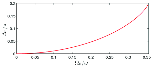
Figure 6: $\Delta\epsilon/\pi$ versus $\Omega_{0}/\omega$.

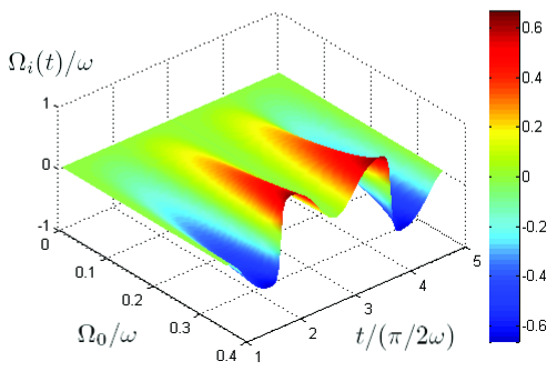
Figure 7: $\Omega_{i}(t)/\omega$ versus $t/(\pi/2\omega)$ and $\Omega_{0}/\omega$.

From Fig. 6, to make the pulses have fewer oscillations, one can increase the ratio $\Omega_{0}/\omega$ to make a population transfer go through fewer pulse periods. On the other hand, according to Fig. 7, the amplitude of $\Omega_{i}(t)$ increases when $\Omega_{0}/\omega$ increases. For $\Omega_{0}$ that satisfies $0\leq\Omega_{0}<\omega/2\sqrt{2}$, we have $|\Omega_{i}(t)|<0.64\omega$ ($\forall t\in[\pi/2\omega,5\pi/2\omega]$). To make the operations simple, $\Omega_{0}/\omega=0.3396$ is chosen, such that $\Delta\epsilon=\pi/6$. Suppose that the parameters in every pulse period repeat the results in $[\pi/2\omega,5\pi/2\omega]$. In this case, if a population transfer starts at $t=\pi/2\omega$, it could be finished at $t=25\pi/2\omega$, i.e., the population transfer goes through 6 pulse periods.

The population of each state is plotted in Fig. 8. Furthermore, in Figs. 9 (a), (b), and (c), $\Omega_{r}(t)$, $\Omega_{i}(t)$ and the detuning $\Delta(t)$ versus $t/(\pi/2\omega)$ during the first pulse period are plotted.

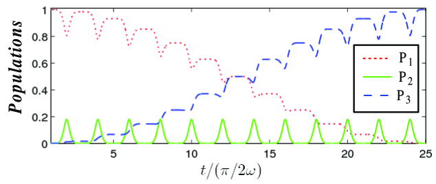
Figure 8: Populations $P_{1}$ (the dotted red line), $P_{2}$ (the solid green line), and $P_{3}$ (the dashed blueline) versus $t/(\pi/2\omega)$ with $\Omega_{0}/\omega=0.3396$.

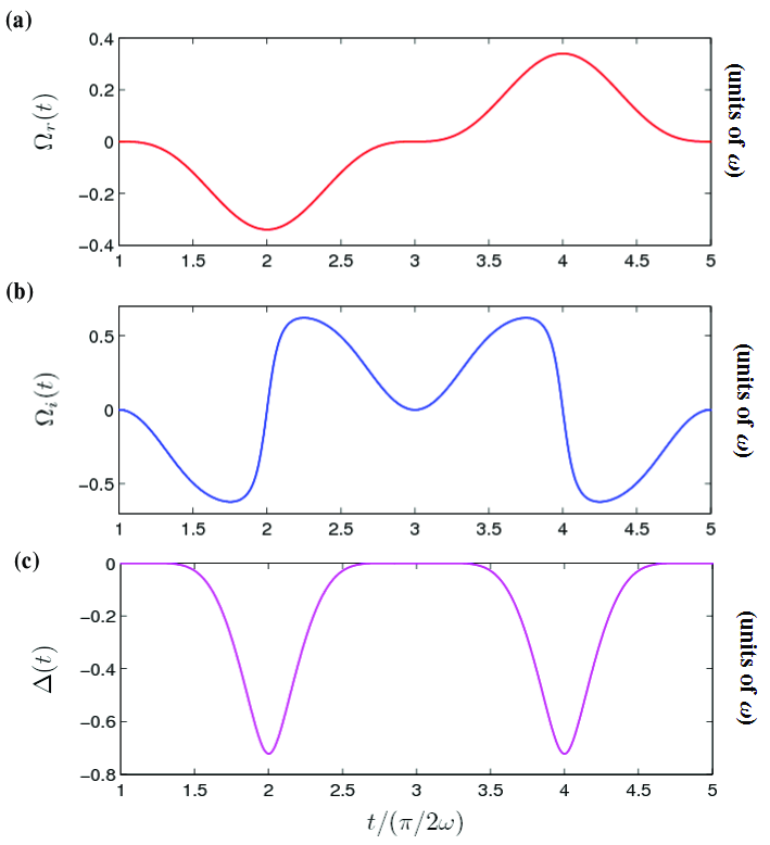
Figure 9: (a) $\Omega_{r}(t)$ versus $t/(\pi/2\omega)$; (b) $\Omega_{i}(t)$ versus $t/(\pi/2\omega)$; (c) $\Delta(t)$ versus $t/(\pi/2\omega)$. ($\Omega_{0}/\omega=0.3396$)

As shown in Fig. 8, the population transfer can be achieved with the designed pulses in this part. However, $P_{3}$ increases up to near unity with greater and greater oscillations. The maximal hump of the oscillations appears at $t=24\pi/2\omega$ with $P_{3}=0.806$. Therefore, the real interaction time $T^{\prime}$ should not approach $24\pi/2\omega$ for a real experiment. To obtained $P_{3}\geq 0.9999$, we require $T^{\prime}\geq 24.71\pi/2\omega$ ($\delta T=|T^{\prime}-T|\leq 1.29\%$). On the other hand, the pulses become weaker and weaker, and they could be turned off smoothly at $t=25\pi/2\omega$. Besides, the curve of $P_{3}$ has a platform at $t=25\pi/2\omega$. Therefore, $P_{3}$ still keeps near unity when $T^{\prime}\geq 25\pi/2\omega$. To summarize, using the approach proposed in this part may have less robustness against the operation errors of the interaction time compared with the approaches of parts A and B. On the other hand, seen from Fig. 9, the real parts and the imaginary parts of pulses are much more smooth compared with that of pulses which were designed in part B. Moreover, since the population transfer goes through only 6 pulse periods, the oscillations of pulses and detunings are much fewer than that of pulses and detunings which were designed in part A. Therefore, the approach of pulse design shown in this section may be more attractive.

For the situation where the total interaction time $T$ is not the integral multiple of a pulse period, e.g., $T=2p\pi/\omega+\tau$, ($p=0,1,2,...$), we can deal with the evolution of the system in the $p$th pulse period by similar way for 1st pulse period. And then, we only need to add pulse design for interval $[T-\tau,T]$ to make population transfers successful at $t=T$.

V Conclusion

In conclusion, we have proposed an invariant-based scheme for pulse design without RWA. First, we found out an invariant for a three-level system without RWA. Then, we exploited the invariant to investigate pulse design for the population transfers in a three-level system. From three different viewpoints, we gave three approaches to design pulses in parts A, B and C of Sec. IV. In part A of Sec. IV, we tried to design pulses with smooth functions. The population transfers could be realized without singularity of pulses. But the pulses would involve many oscillations. In part B of Sec. IV, we tried to reduce the oscillations of pulses by modifying the pulses around their singular points. The oscillations could be reduced a lot, while the population transfers became imperfect and the pulse forms might be complex for the experimental realization. In part C of Sec. IV, instead of choosing control parameters directly, we first chose pulses with feasible forms accompanied with some undetermined coefficients. Then we reversely solved the control parameters. With the help of numerical calculations, we determined all the coefficients of pulses. With the approach shown in part C of Sec. IV, feasible pulses could be designed for every pulse period, and the oscillations of pulses could be well restricted.

Overall, the scheme has shown several novel results and advantages:

(i) To our knowledge, invariants for a three-level system without RWA have not been investigated in the previous schemes. Therefore, the invariant shown in Eq. (11) may be a new one.

(ii) Based on pulse design with the invariant shown in Eq. (11), we do not need any extra couplings.

(iii) The amplitudes of pulses and the maximal values of detunings could be well controlled in the present scheme. But it is difficult for schemes with transitionless quantum driving to do so.

(iv) The pulses designed by the scheme can be smoothly turned on and turned off. Therefore, the scheme should be robust against the fluctuations of parameters.

(v) Compared with adiabatic processes, the system is not required to satisfy the adiabatic condition, thus possessing higher evolution speed.

With these advantages, the scheme may be useful for fast quantum information processing without RWA.

References

- (1) P. Král, I. Thanopulos, and M. Shapiro, Rev. Mod. Phys. 79, 53 (2007).
- (2) K. Bergmann, H. Theuer, and B. W. Shore, Rev. Mod. Phys. 70, 1003 (1998).
- (3) M. P. Fewell, B. W. Shore, and K. Bergmann, Aust. J. Phys. 50, 281 (1997).
- (4) N. V. Vitanov, T. Halfmann, B. W. Shore, and K. Bergmann, Annu. Rev. Phys. Chem. 52, 763 (2001).
- (5) S. B. Zheng, Phys. Rev. Lett. 95, 080502 (2005).
- (6) C. P. Yang, Shih-I Chu, and S. Han, Phys. Rev. Lett. 92, 117902 (2004).
- (7) D. Møler, L. B. Madsen, and K. Mømer, Phys. Rev. A 75, 062302 (2007).
- (8) Z. J. Deng, K. L. Gao, and M. Feng, Phys. Rev. A 74, 064303 (2006).
- (9) M. Demirplak and S. A. Rice, J. Phys. Chem. A 107, 9937 (2003).
- (10) M. V. Berry, J. Phys. A 42, 365303 (2009).
- (11) J. G. Muga, X. Chen, A. Ruschhaupt, and D. Guéry-Odelin, J. Phys. B 42, 241001 (2009).
- (12) J. G. Muga, X. Chen, S. Ibáñez, I. Lizuain, and A. Ruschhaupt, J. Phys. B 43, 085509 (2010).
- (13) X. Chen, A. Ruschhaupt, S. Schmidt, A. del Campo, D. Guéry-Odelin, and J. G. Muga, Phys. Rev. Lett. 104, 063002 (2010).
- (14) X. Chen, I. Lizuain, A. Ruschhaupt, D. Guéry-Odelin, and J. G. Muga, Phys. Rev. Lett. 105 123003 (2010).
- (15) X. Chen and J. G. Muga, Phys. Rev. A 82, 053403 (2010).
- (16) X. Chen, E. Torrontegui, and J. G. Muga, Phys. Rev. A 83, 062116 (2011).
- (17) X. Chen, E. Torrontegui, D. Stefanatos, J. S. Li, and J. G. Muga, Phys. Rev. A 84, 043415 (2011).
- (18) A. del Campo, Phys. Rev. Lett. 111, 100502 (2013).
- (19) A. del Campo, Phys. Rev. A 84, 031606(R) (2011).
- (20) A. del Campo, M. M. Rams, and W. H. Zurek, Phys. Rev. Lett. 109, 115703 (2012).
- (21) A. del Campo, Eur. Phys. Lett. 96, 60005 (2011).
- (22) A. del Campo and M. G. Boshier, Sci. Rep. 2, 648 (2012).
- (23) S. Deffner, C. Jarzynski, and A. del Campo, Phys. Rev. X 4, 021013 (2014).
- (24) J. Zhang, T. H. Kyaw, D. M. Tong, E. Sjövist, and L. C. Kwek, Sci. Rep. 5, 18414 (2015).
- (25) Y. H. Kang, Y. H. Chen, Z. C. Shi, J. Song, and Y. Xia, Phys. Rev. A 94, 052311 (2016).
- (26) X. Chen and J. G. Muga, Phys. Rev. A 86, 033405 (2012).
- (27) Y. H. Chen, Y. Xia, Q. Q. Chen, and J. Song, Phys. Rev. A 89, 033856 (2014).
- (28) X. K. Song, Q. Ai, J. Qiu, and F. G. Deng, Phys. Rev. A 93, 052324 (2016).
- (29) X. K. Song, H. Zhang, Q. Ai, J. Qiu, and F. G. Deng, New J. Phys. 18 023001 (2016).
- (30) S. Ibáñez, X. Chen, E. Torrontegui, J. G. Muga, and A. Ruschhaupt, Phys. Rev. Lett. 109, 100403 (2012).
- (31) S. Ibáñez, X. Chen, and J. G. Muga, Phys. Rev. A 87, 043402 (2013).
- (32) S. Ibáñez and J. G. Muga, Phys. Rev. A 89, 033403 (2014).
- (33) Y. H. Chen, Q. C. Wu, B. H. Huang, Y. Xia, and J. Song, Phys. Rev. A 93, 052109 (2016).
- (34) E. Torrontegui, S. Martínez-Garaot, and J. G. Muga, Phys. Rev. A 89, 043408 (2014).
- (35) S. Martínez-Garaot, E. Torrontegui, X. Chen, and J. G. Muga, Phys. Rev. A 89, 053408 (2014).
- (36) Q. C. Wu, Y. H. Chen, B. H. Huang, J. Song, Y. Xia, and S. B. Zheng, Opt. Express, 24, 22847 (2016).
- (37) Y. H. Kang, Y. H. Chen, Q. C. Wu, B. H. Huang, Y. Xia, and J. Song, Sci. Rep. 6, 30151 (2016).
- (38) A. T. Sornborger, A. N. Cleland, and M. R. Geller, Phys. Rev. A 70, 052315 (2004).
- (39) X. Liu, G. Y. Fang, Q. H. Liao, and S. T. Liu, Phys. Rev. A 90, 062330 (2014).
- (40) D. Sank, Z. Chen, M. Khezri, J. Kelly, R. Barends, B. Campbell, Y. Chen, B. Chiaro, A. Dunsworth, A. Fowler, E. Jeffrey, E. Lucero, A. Megrant, J. Mutus, M. Neeley, C. Neill, P. J. J. O’Malley, C. Quintana, P. Roushan, A. Vainsencher, T. White, J. Wenner, A. N. Korotkov, and J. M. Martinis, Phys. Rev. Lett. 117, 190503 (2016).
- (41) D. Malz and A. Nunnenkamp, Phys. Rev. A 94, 053820 (2016).
- (42) Y. Song, J. P. Kestner, X. Wang, and S. D. Sarma, Phys. Rev. A 94, 012321 (2016).
- (43) S. Hofferberth, B. Fischer, T. Schumm, J. Schmiedmayer, and I. Lesanovsky, Phys. Rev. A 76, 013401 (2007).
- (44) J. Scheuer, X. Kong, R. S. Said, J. Chen, A. Kurz, L. Marseglia, J. Du, P. R. Hemmer, S. Montangero, T. Calarco, B. Naydenov, and F. Jelezko, New J. Phys. 16 093022 (2014)
- (45) J. Chen and L. F. Wei, Phys. Rev. A 91, 023405 (2015).
- (46) S. Ibáñez, Y. C. Li, X. Chen, and J. G. Muga, Phys. Rev. A 92, 062136 (2015).
- (47) H. R. Lewis and W. B. Riesenfeld, J. Math. Phys. 10, 1458 (1969).
- (48) M. Lu, Y. Xia, L. T. Shen, J. Song, and N. B. An, Phys. Rev. A 89, 012326 (2014).
- (49) Y. H. Chen, Y. Xia, Q. Q. Chen, and J. Song, Phys. Rev. A 91, 012325 (2015).
- (50) S. Longhi, Laser Photon. Rev. 3, 243 (2009).
- (51) S. Longhi, J. Phys. B 44, 051001 (2010).
- (52) M. Ornigotti, G. D. Valle, T. T. Fernandez, A. Coppa, V. Foglietti, P. Laporta, and S. Longhi, J. Phys. B 41, 085402 (2008).
- (53) A. A. Rangelov and N. V. Vitanov, Phys. Rev. A 85, 055803 (2012).