Abstract

Community detection is a fundamental unsupervised learning problem for unlabeled networks which has a broad range of applications. Many community detection algorithms assume that the number of clusters $r$ is known apriori. In this paper, we propose an approach based on semi-definite relaxations, which does not require prior knowledge of model parameters like many existing convex relaxation methods and recovers the number of clusters and the clustering matrix exactly under a broad parameter regime, with probability tending to one. On a variety of simulated and real data experiments, we show that the proposed method often outperforms state-of-the-art techniques for estimating the number of clusters.

1 Introduction

As a fundamental problem in network analysis, community detection has drawn much attention from both theorists and practitioners. Most existing methods require the prior knowledge of the true number of clusters, which is often unavailable in real data applications. In this paper we mainly focus on provably estimating the number of clusters in a network.

While it is tempting to use a two-stage procedure [14] where the number of clusters is estimated first and then used as an input for clustering, an erroneous estimation on the number of clusters can deteriorate the clustering accuracy. Instead, we design an algorithm which estimates the true number of clusters and recovers the cluster memberships simultaneously, with provable guarantees.

In this paper, we focus on the widely-used Stochastic Block Models (SBM) [24]. The model assumes the probability of an edge between two nodes are completely determined by the unknown cluster memberships of the nodes. Essentially, this imposes stochastic equivalence, i.e. all nodes in the same cluster behave identically in a probabilistic sense. Despite its simplicity, the SBM is used as a building block in more sophisticated models like the Degree Corrected Block Models [26] and Mixed Membership Block Models [3] and has been applied successfully for clustering real world networks.

Semi-definite programming (SDP) relaxations for network clustering have been widely studied and many different formulations have been proposed. It has been empirically observed that these methods have better clustering performance compared to spectral methods [5, 45, 14]. As shown by [13, 5], SDPs arise naturally when the likelihood of a SBM with equal cluster sizes is relaxed. SDP returns a relaxation of the clustering matrix, which is a $n\times n$ ($n$ being the number of nodes) symmetric matrix whose $ij^{th}$ element is one if nodes $i$ and $j$ belong to the same cluster and zero otherwise. We present a detailed discussion on related work in Section 3. In this work, we use the SDP formulation proposed by [39], which uses a normalized variant of the clustering matrix. Similar relaxations have been used to study $k$-means clustering for sub-gaussian mixtures [34] and SBMs [44].

For community detection in SBM, an algorithm is considered effective if it is asymptotically consistent. There are two types of consistency in the literature. When the number of nodes in the graph is large enough, the network is sufficiently dense, and the signal (usually defined by the separation between intra-cluster probability and inter-cluster probability) is strong enough, strongly consistent methods recover the ground truth labels exactly, while the weakly consistent methods recover a fraction of labels correctly where the fraction approaches one as $n$ goes to infinity.

There have been a number of SDP relaxations for general unbalanced cluster sizes which have been shown to be strongly consistent [40, 19, 9]. One can argue that these methods readily render themselves to estimation of the number of blocks $r$. The idea would be to run the SDP with different values of $r$, and for the correct one the clustering matrix will be the true clustering matrix with high probability. However, all these methods require the knowledge of model parameters. Furthermore, they work in the unequal cluster size setting by introducing an additional penalty term, which requires further tuning. Hence each run with a different choice of $r$ would have an internal tuning step adding to the already expensive computation of the SDP. In this paper, we propose a formulation that is a) entirely tuning free when the number of clusters is known, and b) when it is unknown, is able to recover the number of clusters and the clustering matrix in one shot.

Furthermore, our method provably works in the weakly assortative setting, whereas the usual necessary separation condition for recovery is that the maximal inter-cluster connecting probability (think of this as noise) is smaller than the minimal intra-cluster connecting probability (the signal) by a certain margin. This separation condition is known as strong assortativity. In contrast, our work only requires that for each node, the probability of connecting to the nodes in its own cluster is greater by a margin than the largest probability of connecting with nodes in other clusters. This property is called weak assortativity. It is not hard to see that weakly assortative models are a superset of strongly assortative models. Weak assortativity was first introduced in [5], who establish exact recovery under this weaker condition for SDPs for blockmodels with equal sized communities.

In Sec 5 we sketch a rather interesting empirical property of our algorithm (also pointed out in [40]); namely it can identify different granularities of separations as a byproduct. For example, the tuning phase, which we sketch in Section 5, finds different substructures of the network as it searches over different tuning parameters. For example, if there are $K$ meta clusters which are more well separated than the rest, then as we tune, we will first find these meta-clusters, and then finer substructures within them. While this is not the main goal of our paper, it indeed makes our approach ideal for exploratory analysis of networks. We also leave the theoretical analysis of finding multi-resolution clusterings for future work.

We will formalize these concepts in Section 2 and discuss the related work in more detail in Section 3. Section 4 contains our main theoretical contributions and finally, in Section 5 we demonstrate the efficacy of our algorithm compared to existing methods on a variety of simulated and real networks.

2 Problem Setup and Notations

Assume $(S_{1},\cdots,S_{r})$ represent a $r$-partition for $n$ nodes $\{1,\cdots,n\}$. Let $m_{i}=|S_{i}|$ be the size of each cluster, and let $m_{\min}$ and $m_{\max}$ be the minimum and maximum cluster sizes respectively. We denote by $A$ the $n\times n$ binary adjacency matrix with the true and unknown membership matrix $Z=\{0,1\}^{n\times r}$,

$$P(A_{ij}=1|Z)=Z_{i}^{T}BZ_{j}\quad\forall i\neq j, B,Z$$ (SBM())

$$P(A_{ii}=0)=1,\quad Z^{T}Z=diag(\bm{m}),$$ (1)

where $B$ is a $r\times r$ matrix of within and across cluster connection probabilities and $\bm{m}$ is a length $r$ vector of cluster sizes. The elements of $B$ can decay with graph size $n$. In this paper we focus on the regime where the average expected degree grows faster than logarithm of $n$. In this regime, it is possible to obtain strong or weak consistency.

Given any block model, the goal for community detection is to recover the column space of $Z$. For example if we can solve $ZZ^{T}$ or its normalized variant $Zdiag(\bm{m})^{-1}Z^{T}$, then the labels can be recovered from the eigenvectors of the clustering matrix.

The normalized clustering matrix:

In this paper we focus on recovering the following normalized version:

$$X_{0}=Z\text{diag}(\bm{m})^{-1}Z^{T}$$ (2)

It can be easily checked that $X_{0}\textbf{1}_{n}=\textbf{1}_{n}$, since $Z\textbf{1}_{k}=\textbf{1}_{n}$. Furthermore, $X_{0}$ is positive semi-definite and its trace (which equals its nuclear norm as well) equals the number of clusters $r$.

Assortativity (strong vs. weak):

Assortativity is a condition usually required in membership recovery. The strong assortativity (see Eq. (3)) requires the smallest diagonal entry to be greater than the largest off-diagonal entry.

$$\min_{k}B_{kk}-\max_{k\neq\ell}B_{k\ell} >0$$ (3)

$$\min_{k}\left(B_{kk}-\max_{\ell\neq k}B_{k\ell}\right) >0.$$ (4)

[5] first introduces an SDP that provably achieves exact recovery for weakly assortative models (Eq. (4)) with equal cluster sizes, i.e., compared with (3), weak assortativity only compares the probability within the same row and column; it requires that any given cluster $k$, should have a larger probability of connecting within itself than with nodes in any other cluster. It is easy to check that strong assortativity indicates weak assortativity and not vice versa.

For any matrix $X\in\mathbb{R}^{n\times n}$, denote $X_{S_{k}S_{\ell}}$ as the submatrix of $X$ on indices $S_{k}\times S_{\ell}$, and $X_{S_{k}}:=X_{S_{k}\times S_{k}}$. Let 1 be all one vector, and $\textbf{1}_{S_{k}}\in\mathbb{R}^{n}$ be the indicator vector of $S_{k}$, equal to one on $S_{k}$ and zero elsewhere. The inner product of two matrices is defined as $\langle{A},{B}\rangle=\text{trace}(A^{T}B)$. We use $\circ$ to denote the Schur (elementwise) product of two matrices. Standard notations for complexity analysis $o,O,\Theta,\Omega$ will be used. And those with a tilde are to represent the same order ignoring log factors.

3 Related Work

While most community detection methods assume that the number of communities ($r$) is given apriori, there has been much empirical and some theoretical work on estimating $r$ from networks.

Methods for estimating $r$: A large class of methods chooses $r$ by maximizing some likelihood-based criterion. While there are notable methods for estimating $r$ for non-network structured data from mixture models [38, 21, 7, 37], we will not discuss them here.

Many likelihood-based methods use variants or approximations of Bayesian Information Criterion (BIC); BIC, while a popular choice for model selection, can be computationally expensive since it depends on the likelihood of the observed data. Variants of the Integrated Classification Likelihood (ICL, originally proposed by [7]) were proposed in [15, 27]. Other BIC type criteria are studied in [32, 42, 33].

In [23] a computationally efficient variational Bayes technique is proposed to estimate $r$. This method is empirically shown to be more accurate than BIC and ICL and faster than Cross Validation based approaches [11]. A Bayesian approach with a new prior and an efficient sampling scheme is used to estimate $r$ in [41]. While the above methods are not provable, a provably consistent likelihood ratio test is proposed to estimate $r$ in [43].

Another class of methods is based on the spectral approach. The idea is to estimate $r$ by the number of “leading eigenvalues” of a suitably normalized adjacency matrix  [36, 25, 10, 16]. Of these the USVT estimator [10] uses random matrix theory to estimate $r$ simply by thresholding the empirical eigenvalues of the adjacency matrix appropriately. In [8] it is shown that the informative eigenvalues of the non-backtracking matrix are real-valued and separated from the bulk under the SBM. In [28], the spectrum of the non-backtracking matrix and the Bethe-Hessian operator are used to estimate $r$, the later being shown to work better for sparse graphs.

[1] proposes a degree-profiling method achieving the optimal information theoretical limit for exact recovery. This agnostic algorithm first learns a preliminary classification based on a subsample of edges, then adjust the classification for each node based on the degree-profiling from the preliminary classification. However it involves a highly-tuned and hard to implement spectral clustering step (also noted by [40]). It also requires specific modifications when applied to real world networks (as pointed out by the authors) .

In [47], communities are sequentially extracted from a network; the stopping criterion uses a bootstrapped approximation of the null distribution of the statistic of choice. In  [6], the null distribution of a spectral test statistic is derived, which is used to test $r=1$ vs $r>1$ at each step of a recursive bipartitioning algorithm. A generalization of this approach for testing a null hypothesis for $r$ blocks can be found in [30]. While the algorithm in [6] often produces over-estimates of $r$, [30]’s hypothesis test depends on a preliminary fitting with an algorithm which exactly recovers the parameters. The final accuracy heavily depends on the accuracy of this fit. Network cross-validation based methods have also been used for selecting $r$. The cross-validation can be carried out either via node splitting [3], or node-pair splitting [22, 11]; the asymptotic consistency of these methods are shown in [11]. We conclude with a comparison of our approach to other convex relaxations.

Comparison to other convex relaxations

In recent years, SDP has drawn much attention in handling community detection problems with Stochastic Block Models. Various of relaxations have been shown to possess strong theoretical guarantees in recovering the true clustering structure without rounding [5, 19, 20, 9, 40, 35, 18]. Most of them aim at recovering a binary clustering matrix, and show that the relaxed SDP will have the ground truth clustering matrix as its unique optimal solution. For unbalanced cluster sizes, an extra penalization is often introduced which requires additional tuning [9, 19, 40]. While one can try different choices of $r$ for these SDPs until achieving exact recovery, the procedure is slower since each run would need another internal tuning step.

SDP with a normalized clustering matrix was introduced by [39]. They have been used for network clustering [44] and for the relaxation of $k$-means clustering of non-network structured data [39, 34] .

$$\begin{split}\max&\quad\langle{A},{X}\rangle\\ s.t.&\quad X\succeq 0,X\geq 0,\\ &\quad X\textbf{1}=\textbf{1},\text{trace}(X)=r\end{split}$$ (SDP-PW)

However the formulation in [44] requires an additional parameter as an lower bound on the minimum size of the clusters; loose lower bounds can empirically deteriorate the performance. Also the authors only establish weak consistency of the solution.

Some of these methods do not require the knowledge of $r$ in the constraints, but instead have the dependency implicitly. In [12] a convexified modularity minimization for Degree-corrected SBM is proposed, which also works for SBMs as a special case of degree corrected models. The authors suggest one over total number of edges as the default value for the tuning parameter, but when dealing with delicate structures of the network, this suggested value can be sub-optimal and further tuning is required. The procedure also requires $r$ for the final clustering of the nodes via Spectral Clustering from the clustering matrix.

A different convex relaxation motivated by low-rank matrix recovery is studied in [14]. Here, first the eigenspectrum of $A$ is used to estimate $r$, which is subsequently used to estimate tuning parameters required in the main algorithm. We can also tune the tuning parameter with other heuristics, but as the theorem in that paper implies, the tuning parameter needs to lie between the minimal intra-cluster probabilities and maximal inter-cluster probabilities, which is only feasible for strongly assortative settings. We provide more details in the experimental section.

Hierarchical clustering structures

A phenomenon that has been observed [40, 14] is that convex relaxations can be used to find hierarchical structures in the networks by varying the tuning parameter. In the experimental section we demonstrate this with some examples.

Separation conditions

In terms of the separation conditions, most aforementioned convex relaxations are consistent in the dense regime under strong assortativity except [5] and [44]. However, [5] only prove exact recovery of clusters for equal sized clusters, whereas [44] only show weak consistency and require the knowledge of additional parameters like the minimum cluster size. [40] shows exact recovery while matching the information theoretical lower bound, which is not the goal of this paper.

In this paper, we compare our algorithm with noted representatives from the related work. From the Spectral methods, we compare with the USVT estimator and the Bethe Hessian based estimator [28], which has been shown to empirically outperform a variety of other provable techniques like [43] and [11]. For these methods, we first estimate $r$ and then use the Regularized Spectral Clustering [4, 29] algorithm to obtain the final clustering. From the convex relaxation literature, we compare with [14] and [12], neither of which require $r$ for estimating the clustering except for the final clustering step.

4 Main Result

In various SDP relaxations for community detection under SBMs, the objective function is taken as the linear inner product of the adjacency matrix $A$ and the target clustering matrix $X$, some formulations also have some additional penalty terms. The inner product objective can be derived from several different metrics for the opitimality of the clustering, such as likelihood or modularity. The penalty terms vary depending on what kind of a solution the SDP is encouraged to yield. For example, in low-rank matrix recovery literature, it is common practice to use the nuclear norm regularization to encourage low-rank solution. For a positive semi-definite matrix, the nuclear norm is identical to its trace. When the number of clusters $r$ is unknown, we consider the following SDP.

$$\begin{split}\max&\quad\text{trace}(AX)-\lambda\text{trace}(X)\\ s.t.&\quad X\succeq 0,X\geq 0,X\textbf{1}=\textbf{1},\end{split} \lambda$$ (SDP-)

where $\lambda$ is a tuning parameter, and $X\geq 0$ is an element-wise non-negativity constraint. The following theorem guarantees the exact recovery of the ground truth solution matrix, when $\lambda$ lies in the given range for the tuning parameter.

Theorem 1.

Let $\hat{X}$ be the optimal solution of (SDP-$\lambda$) for $A\sim\text{SBM}(B,Z)$ where $m_{\min}$ and $m_{\max}$ denote the smallest and largest cluster sizes respectively. Define the separation parameter $\delta=\min_{k}(B_{kk}-\max_{\ell\neq k}B_{k\ell})$. If

$$c_{1}\max_{k}\sqrt{m_{k}B_{kk}}+c_{2}\sqrt{n\max_{k\neq\ell}B_{k\ell}}\leq\lambda$$

$$\qquad\leq m_{\min}\left(\delta-\max_{k,\ell}\sqrt{\frac{B_{k\ell}\log m_{k}}{m_{k}}}\right)$$

then $\hat{X}=X_{0}$ with probability at least $1-n^{-1}$ provided

$$\delta\geq 2\sqrt{6\log n}\max_{k}\sqrt{\frac{B_{kk}}{m_{k}}}+ 6\max_{\ell\neq k}\sqrt{\frac{B_{k\ell}\log n}{m_{\min}}}$$

$$+\frac{c\sqrt{np_{\max}}}{m_{\min}}$$ (5)

Remark 1.

The above theorem controls how fast the different parameters can grow or decay as $n$ grows. For ease of exposition, we will discuss these constraints on each parameter by fixing the others. The number of clusters $r$ can increase with $n$. In the dense setting, when $B_{kk}=\Theta(1)$, $m_{\min}=\omega(\sqrt{n})$ and $r=o(\sqrt{n})$, which matches with the best upper bound on $r$ from existing literature. Finally when $\max_{k}B_{kk}=\Theta(\log n/n)$, we note that $m_{\min}=\tilde{\Theta}(n)$ and $r=\tilde{\Theta}(1)$.

We can see from the condition in Theorem 1 that the tuning parameter should be of the order $\sqrt{d}$ where $d$ is the average degree. In fact, as shown in the following theorem, when the $\lambda$ is greater than the operator norm, (SDP-$\lambda$) returns a degenerating rank-1 solution. This gives an upper bound for $\lambda$.

Proposition 1.

When $\lambda\geq\|A\|_{op}$, then the solution for (SDP-$\lambda$) is $\textbf{1}\textbf{1}^{T}/n$.

The proof of Proposition 1 is to be found in Appendix B. Recall the properties of the ground truth clustering matrix defined in Eq. (2). If the optimal solution recovers the ground truth $X_{0}$ exactly, we can estimate $r$ easily from its trace. Therefore we have the following corollary.

Corollary 1.

Let $\hat{X}$ be the optimal solution of (SDP-$\lambda$) with $A\sim\text{SBM}(B,Z)$, where $B\in[0,1]^{r\times r}$. Under the condition in Theorem 1, $\text{trace}(\hat{X})=r$ with probability at least $1-n^{-1}$.

In particular, when $r$ is known, we have the following exact recovery guarantee, which is stronger than the weak consistency result in [44].

Theorem 2.

Let $A\sim\text{SBM}(B,Z)$, where $B\in[0,1]^{r\times r}$. $X_{0}$ is the optimal solution of (SDP-PW) with probability at least $1-n^{-1}$, if the separation condition Eq. (5) holds true.

We can see that the two SDPs (SDP-$\lambda$) and (SDP-PW) are closely related. In fact, the Lagrangian function of (SDP-PW) is same as the Lagrangian function of (SDP-$\lambda$) if we take the lagrangian multiplier for the constraint $\text{trace}(X)=r$ as $\lambda$. We use this fact in the proof of Theorem 1. Both proofs rely on constructing a dual certificate witness, which we elaborate in the following subsection.

4.1 Dual Certificate Witness

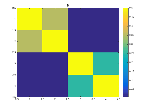
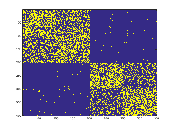
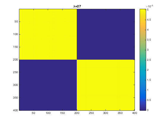
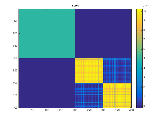
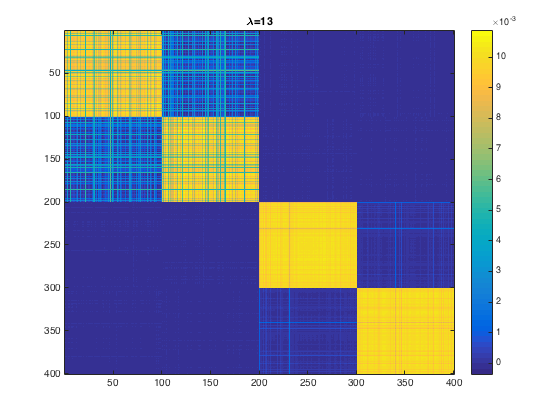
(a) $B$	(b) Adjacency	(c) $\lambda=27$	(d) $\lambda=21$	(e) $\lambda=13$.

Figure 1: Solution matrices with various choices of $\lambda$.

In this sketch we develop the sufficient conditions with a certain construction of the dual certificate which guarantees $X_{0}$ to be the optimal solution. We derive the main conditions and leave the technical details to the supplementary materials. To start with, the KKT conditions of (SDP-PW) can be written as below.

First Order Stationary

$$\quad-A-\Lambda+(1\alpha^{T}+\alpha 1^{T})+\beta I-\Gamma=0$$ (6)

Primal Feasibility

$$\quad X\succeq 0,\ 0\leq X\leq 1,\ X\textbf{1}_{n}=\textbf{1}_{n},\ \text{trace}(X)=r$$ (7)

Dual Feasibility

$$\quad\Lambda\succeq 0,\ \ \Gamma\geq 0$$ (8)

Complementary Slackness

$$\quad\langle{\Lambda},{X}\rangle=0,\ \ \Gamma\circ X=0$$ (9)

For (SDP-$\lambda$), we replace $\beta$ by $\lambda$ and drop the trace constraint in the primal feasibility. Since we use $X_{0}$ as the primal construction, removing one primal feasibility condition has no impact on the other part of the proof.

Consider the following primal-dual construction.

$$X_{S_{k}}=E_{m_{k}}/m_{k};\quad X_{S_{k}S_{\ell}}=0,\forall k\neq\ell$$ (10)

$$\Lambda_{S_{k}}=-A_{S_{k}}+(1_{m_{k}}\alpha_{S_{k}}^{T}+\alpha_{S_{k}}1_{m_{k}}^{T})+\beta I_{m_{k}},$$

$$\Lambda_{S_{k}S_{\ell}}=-(I-\frac{E_{m_{k}}}{m_{k}})A_{S_{k}S_{\ell}}(I-\frac{E_{m_{\ell}}}{m_{\ell}})$$ (11)

$$\Gamma_{S_{k}}=0,$$

$$\Gamma_{S_{k},S_{\ell}}=-A_{S_{k},S_{\ell}}-\Lambda_{S_{k},S_{\ell}}+(1_{m_{k}}\alpha_{S_{\ell}}^{T}+\alpha_{S_{k}}1_{m_{\ell}}^{T})$$ (12)

$$\alpha_{S_{k}}=\frac{1}{m_{k}}\left(A_{S_{k}}\textbf{1}_{m_{k}}+\phi_{k}\textbf{1}_{m_{k}}\right)$$ (13)

$$\phi_{k}=-\frac{1}{2}\left(\beta+\frac{\textbf{1}_{m_{k}}^{T}A_{S_{k}}\textbf{1}_{m_{k}}}{m_{k}}\right)$$ (14)

The first order condition Eq. (6) is satisfied by construction. By Eq. (13) and (14), it can be seen that

$$\alpha_{S_{k}}^{T}\textbf{1}_{m_{k}}=\frac{1}{m_{k}}\left(\textbf{1}_{m_{k}}^{T}A_{S_{k}}\textbf{1}_{m_{k}}\right)+\phi_{k}=\frac{\textbf{1}_{m_{k}}^{T}A_{S_{k}}\textbf{1}_{m_{k}}}{2m_{k}}-\frac{\beta}{2}$$

In view of the fact that both $\Lambda$ and $X$ are positive semi-definite, $\langle{\Lambda},{X}\rangle=0$ is equivalent to $\Lambda X=0$. Now it remains to verify:

$$(a)\ \Lambda X=0;\qquad(b)\ \Lambda\succeq 0;\qquad(c)\ \Gamma_{uv}\geq 0,\forall u,v$$

And it can be seen that (a) holds by construction.

Positive Semidefiniteness of $\Lambda$

For (b), since span$(\textbf{1}_{S_{k}})\subset\text{ker}(\Lambda)$, it suffices to show that for any $u\in\text{span}(\textbf{1}_{S_{k}})^{\perp}$, $u^{T}\Lambda u\geq\epsilon\|u\|^{2}$. Consider the decomposition $u=\sum_{k}u_{S_{k}}$, where $u_{S_{k}}:=u\circ\textbf{1}_{S_{k}}$, and $u_{S_{k}}\perp\textbf{1}_{m_{k}}$.

$$u^{T}\Lambda u=\sum_{k}u_{S_{k}}^{T}\Lambda_{S_{k}}u_{S_{k}}+\sum_{k\neq\ell}u_{S_{k}}^{T}\Lambda_{S_{k}S_{\ell}}u_{S_{\ell}}$$

$$= -\sum_{k}u_{S_{k}}^{T}A_{S_{k}}u_{S_{k}}+\beta\sum_{k}u_{S_{k}}^{T}u_{S_{k}}-\sum_{k\neq\ell}u_{S_{k}}^{T}A_{S_{k}S_{\ell}}u_{S_{\ell}}$$

$$= -\sum_{k}u_{S_{k}}^{T}(A-P)_{S_{k}}u_{S_{k}}$$

$$\qquad\qquad-\sum_{k\neq\ell}u_{S_{k}}^{T}(A-P)_{S_{k}S_{\ell}}u_{S_{\ell}}+\beta\|u\|_{2}^{2}$$

$$= -u^{T}Au+\beta\|u\|_{2}^{2}\geq\epsilon\|u\|^{2}$$

In order to obtain a sufficient condition on $\beta$, we will use the following lemma from Theorem 5.2 of [31], which provides a tight bound for the spectral norm $\|A-\mathbb{E}A\|$ for stochastic block models.

Lemma 1 ([31] Theorem 5.2).

Let $A$ be the adjacency matrix of a random graph on $n$ nodes in which edges occur independently. Set $\mathbb{E}A=P=(p_{ij})$ and assume that $n\max_{ij}p_{ij}\leq d$ for $d\geq c_{0}\log n$ and $c_{0}>0$. Then, for any $r>0$ there exists a constant $C=C(r,c_{0})$ such that $\|A-P\|\leq C\sqrt{d}$, with probability at least $1-n^{-r}$.

By Lemma 1, a sufficient condition is to have

$$\beta=\Omega(\sqrt{np_{\max}})\geq\|A-P\|_{2}$$ (15)

Positiveness of $\Gamma$

For (c), denote $d_{i}(S_{k})=\sum_{j\in S_{k}}A_{i,j}$, which is the number of edges from node $i$ to cluster $k$, and $\bar{d}_{i}(S_{k})=\frac{d_{i}(S_{k})}{m_{k}}$. Define the average degree between two clusters as $\bar{d}(S_{k}S_{\ell})=\frac{\sum_{i\in S_{\ell}}d_{i}(S_{k})}{m_{\ell}}$. For $k\neq\ell$, $u\in C_{k},v\in C_{\ell}$, we have $\Gamma_{uv}\geq 0$ equivalent to

$$\bar{d}_{u}(S_{k})-\bar{d}_{u}(S_{\ell})+\frac{1}{2}\left(\bar{d}(S_{k}S_{\ell})-\bar{d}(S_{k}S_{k})\right)$$

$$+\bar{d}_{v}(S_{\ell})-\bar{d}_{v}(S_{k})+\frac{1}{2}\left(\bar{d}(S_{k}S_{\ell})-\bar{d}(S_{\ell}S_{\ell})\right)$$

$$-\frac{\beta}{2m_{\ell}}-\frac{\beta}{2m_{k}}\geq 0$$ (16)

By Chernoff bound and union bound, we have a sufficient condition of $\Gamma_{uv}\geq 0$ for all pairs of $(u,v)$:

$$\delta\geq 2\sqrt{6\log n}\max_{k}\sqrt{\frac{B_{kk}}{m_{k}}}+\max_{\ell\neq k}6\sqrt{\frac{B_{k\ell}\log n}{m_{\min}}}+c\frac{np_{\max}}{m_{\min}}$$

A complete proof could be found in Appendix A.

5 Experiments

First, we present a procedure for tuning $\lambda$ in (SDP-$\lambda$) in subsection 5.1. Then, in subsection 5.2 and 5.3 we present results on simulated and real data.

5.1 Tuning and substructure finding

  Input: graph $A$, number of candidates $T$;

  for i = 0:T-1 do

     $\lambda=\exp(\frac{i}{T}\log(1+\|A\|_{op}))-1$;

     $\hat{X}_{\lambda}=$ solution of (SDP-$\lambda$).

     $\theta(\lambda)=\frac{\sum_{i\leq r_{\lambda}}\sigma_{i}(X_{\lambda})}{\text{trace}(\hat{X}_{\lambda})}$;

  end for

  $\hat{\lambda}=\arg\max_{\lambda}\theta(\lambda)$;

  Output: $\hat{X}_{\hat{\lambda}}$, $\hat{r}=[\text{trace}(\hat{X}_{\hat{\lambda}})]$;

Algorithm 1 Semidefinite Program with Unknown $r$ (SPUR)

As shown in Proposition 1, choice of $\lambda$ should not exceed the operator norm of the observed network. Therefore we do a grid search for $\lambda$ from 0 to $\|A\|_{op}$ in log scale. For each candidate $\lambda$, we solve (SDP-$\lambda$) and get the corresponding solution $\hat{X}_{\lambda}$. The estimated number of clusters is defined as $r_{\lambda}=[\text{trace}(\hat{X}_{\lambda})]$, where $[\cdot]$ represent the rounding operator. Let $\sigma_{i}(X)$ be the $i$-th eigenvalue of $X$. We then pick the solution which maximizes the proportion of leading eigenvalues $\hat{\lambda}=\arg\max_{\lambda}\sum_{i\leq r_{\lambda}}\sigma_{i}(\hat{X}_{\lambda})/\text{trace}(\hat{X}_{\lambda})$. This fraction calculates the proportion of leading eigenvalues in the entire spectrum. If it equals to one, then the solution is low rank. The algorithm is summarized in Algorithm 1. In the experiments, for scalability concerns we fix a smaller range and search over the range $0.1\sqrt{\bar{d}}$ to $2\sqrt{\bar{d}}$, where $\bar{d}$ denotes the average degree.

In theory, when $\lambda$ lies in the interval specified by Corollary 1 exact recovery is possible. Yet, in practice, solutions with different choices of $\lambda$, even outside of the theoretical range, still gives us some useful information about the sub-structures of the network. Figure 1 shows a probability matrix which has large separation into two big clusters and each further splits into two smaller clusters with different separations. With a larger $\lambda$ it returns an under estimated $r$, but consistent to the hierarchical structure in the original network. In this vein, the tuning method provides a great way to do exploratory analysis of the network.

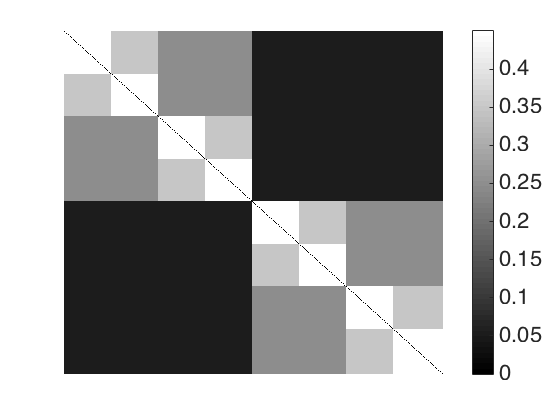
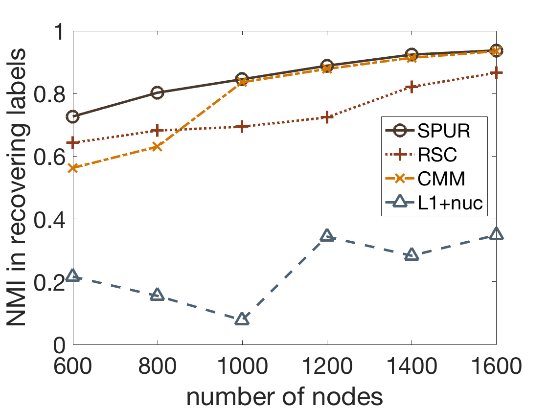
(a) Expectation of network:	(b) NMI;

Figure 2: The expectation matrix and NMI used for the known $r$ setting.

5.2 Synthetic data

We present our simulation results in three parts - known $r$, increasing $r$ and unknown $r$. We report the normalized mutual information (NMI) of predicted label and ground truth membership, and the accuracy of estimating $r$. For each experiment, the average over 10 replicates is reported.

Known number of clusters

We compare the NMI of SPUR against some state-of-the-art methods, including Regularized Spectral Clustering (RSC) [4], and two convex relaxations which do not require $r$ as input to the optimization: convexified modularity maximization (CMM) in [12]; and the $\ell_{1}$ plus nuclear norm penalty method proposed in [14] (L1+nuc). In this setting, we use (SDP-PW) directly which does not involve any tuning. In contracst, due to the hierarchical structure of the network, the default values for the tuning parameters in both methods would only be able to recover the lowest level of hierarchy, which consists of two clusters. Hence for a fair comparison, we try a grid search for those tuning parameters and choose the one that gives largest eigengap between the $r$-th and $r+1$th eigenvalues of the clustering matrices. The expectation of the network generated is shown in the left panel of Figure 2. The right panel shows that the proposed method outperforms the competing methods.

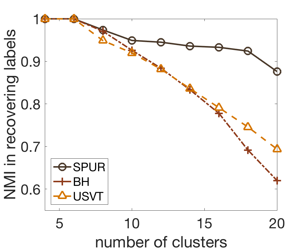
Figure 3: NMI under planted partition model with increasing (unknown) number of clusters.

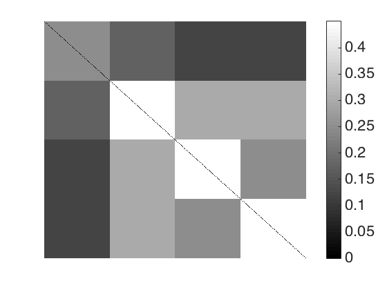
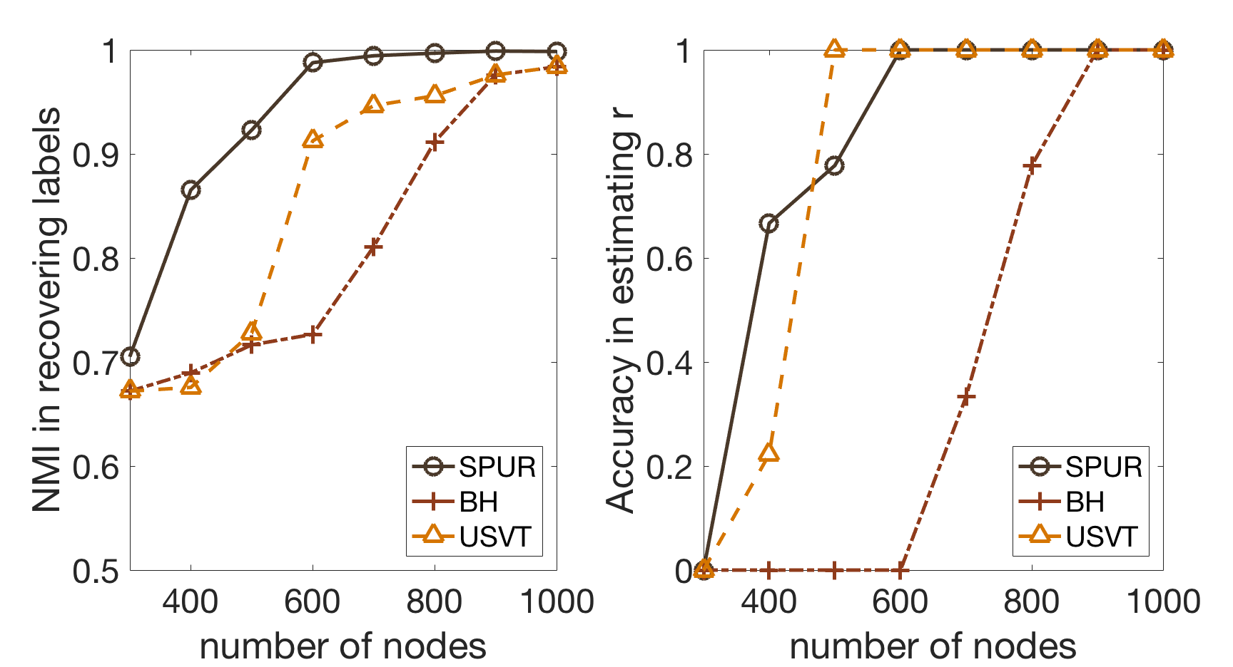
(a) balanced setting with unknown $r$:	NMI	Accuracy of $r$.
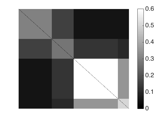
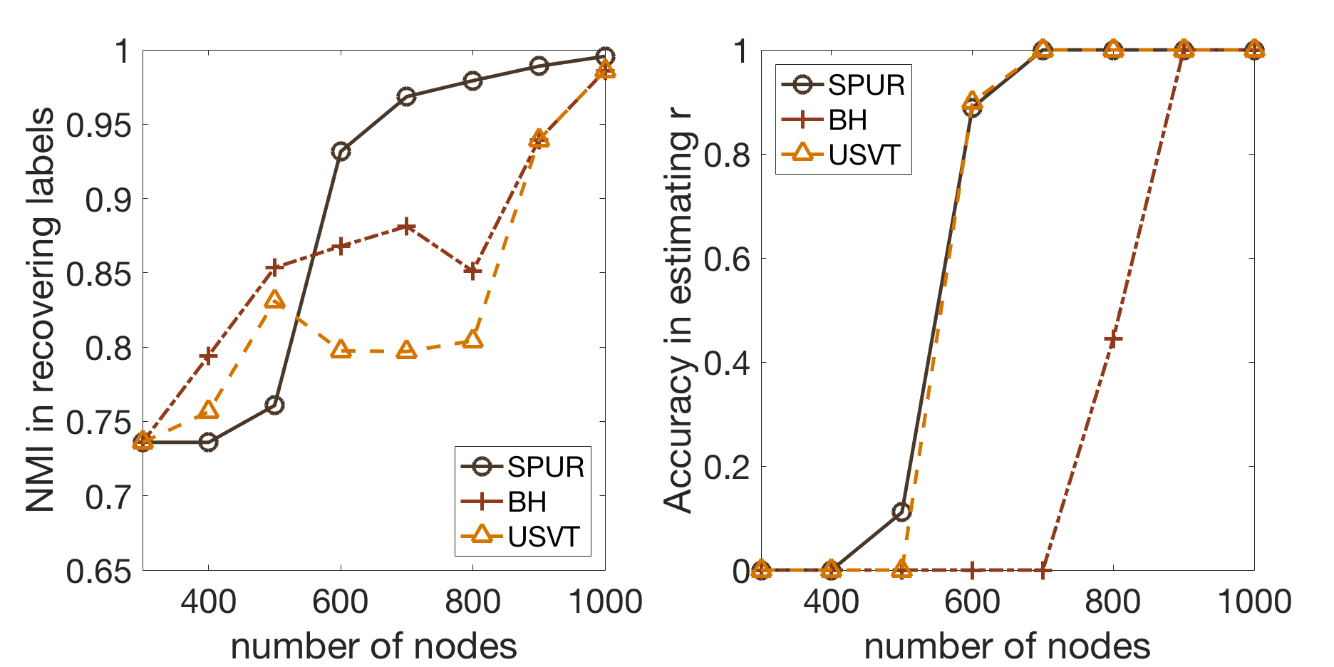
(b) unbalanced setting with unknown $r$:	NMI	Accuracy of $r$.

Figure 4: The first row shows weakly assortative models with balanced cluster sizes and the corresponding NMI and accuracy in estimating $r$; the second row shows those for unbalanced cluster sizes.

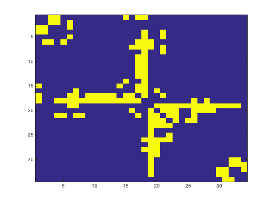
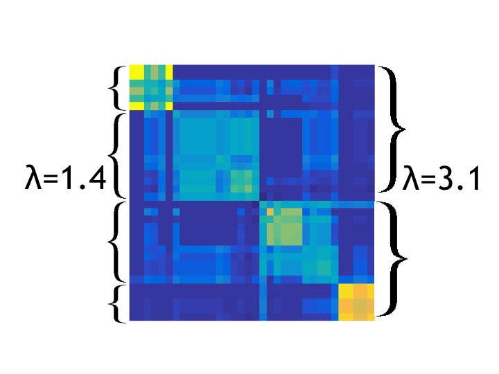
Figure 5: Adjacency matrix and predicted $X$ for karate club dataset; ordered by predicted labels.

Increasing number of clusters

In this experiment, we fix the number of nodes as 400 and increase the number of clusters from 4 to 20. With each given $r$ we generate the graph with $B_{kk}=0.6,B_{k\ell}=0.1,\forall k\neq\ell$ and $m_{\max}/m_{\min}=4$, then run the various estimation algorithms same as in previous experiment. It is shown in 3 that as number of clusters increases, all methods deteriorate, but the performance for SPUR declines slower than the others.

Unknown number of clusters

In this experiment, we carry out two synthetic experiments for weakly assortative graphs for both balanced and unbalanced cluster sizes. We generate the network with expectation matrices shown in the leftmost column of Figure 4, and show the NMI of predicted labels with ground truth labels, and the fraction of returning the correct $r$, for both balanced (Figure 4-(a)) and unbalanced (Figure 4-(b)) settings. We run SPUR and compare the result with 1) the Bethe-Hessian estimator (BH) in [28], in particular BHac (which has been shown to perform better for unbalanced settings), 2) USVT in [10].For all competing methods, we run spectral clustering with the estimated $r$ to estimate the cluster memberships. As we can see here, SPUR has a better accuracy in label recovery than competing methods. SPUR also achieves accurate cluster number faster than competing methods.

Table 1: Estimated number of clusters for real networks.

Datasets	Truth	SDP	BH	USVT	CMM
College Football	12	13	10	10	10
Political Books	3	3	4	4	2
Political Blogs	2	3	8	3	2
Dolphins	2	5	2	4	7
Karate	2	2	2	2	2

5.3 Real Datasets

We apply the proposed method on several real world data sets: the college football dataset [17], the political books, political blogs [2], dolphins and karate club [46] datasets. We compare the performance of SPUR with BH, CMM and USVT in Table 1. As seen from [28], most algorithm correctly finds $r$ for about 2 or 3 of these networks. It is also worth pointing out that this typically happens because different techniques finds different clusterings of the hidden substructures [6]. We will now show one such substructure we found in the Karate club data.

Figure 5 shows the adjacency matrix and $\hat{X}$ for the Karate club data set. For $\lambda=3.1$, we find two clusters, whereas for $\lambda=1.4$, we find 4 clusters, which are further subdivisions of the first level. While our tuning method picks up $\lambda=3.1$ ($r=2$) based on the scoring, we show the substructure for $\lambda=1.4,r=4$ in Figure 5. The left panel shows the adjacency matrix of the Karate club data ordered according to the clusters obtained with $\lambda=1.4$. The right panel of Figure 5 shows finer substructure of $\hat{X}$; as suggested by the adjacency matrix, within each group there are two small clique like groups at the two corners, and the hubs from each group.

6 Conclusion

We present SPUR, a SDP-based algorithm which provably learns the number of clusters $r$ in a SBM under the weakly assortative setting. Our approach does not require the knowledge of model parameters, and foregoes the added tuning step used by existing SDP approaches for unequal size clusters when $r$ is known. For unknown $r$, the tuning in the objective provides guidance in exploring the finer sub-structure in the network. Simulated and real data experiments show that SPUR performs comparably or better than state-of-the-art approaches.

Acknowledgements

PS was partially supported by NSF grant DMS 1713082.

Appendix A Proof of Theorem 1 and 2

Proof of Theorem 2.

The construction (11)-(14) together with $X_{0}$ is a primal-dual certificate, if (6)-(9) are satisfied. In view of the fact that both $\Lambda$ and $X$ are positive semi-definite, $\langle{\Lambda},{X}\rangle=0$ is equivalent to $\lambda X=0$. We need to check the following:

• $\Lambda X=0$;

• $\Lambda\succeq 0$;

• $\Gamma_{uv}\geq 0,\forall u,v$.

Note that span$(X)$=span$(\textbf{1}_{S_{k}})$, therefore we only need to show $\Lambda\textbf{1}_{S_{k}}=0,\forall k\in[r]$. Or equivalently $\Lambda_{S_{k}}\textbf{1}_{m_{k}}=0$ and $\Lambda_{S_{k}S_{\ell}}\textbf{1}_{m_{\ell}}=0$. The latter holds by (11). For the former, recall that $\alpha_{S_{k}}^{T}\textbf{1}_{m_{k}}=\frac{1}{m_{k}}\left(\textbf{1}_{m_{k}}^{T}A_{S_{k}}\textbf{1}_{m_{k}}\right)+\phi_{k}$.

$$0= \Lambda_{S_{k}}\textbf{1}_{m_{k}}=-A_{S_{k}}\textbf{1}_{m_{k}}+(\textbf{1}_{m_{k}}\alpha_{S_{k}}^{T}\textbf{1}_{m_{k}}+\alpha_{S_{k}}\textbf{1}_{m_{k}}^{T}\textbf{1}_{m_{k}})+\beta\textbf{1}_{m_{k}}$$

$$= -A_{S_{k}}\textbf{1}_{m_{k}}+\left(\frac{\textbf{1}_{m_{k}}^{T}A_{S_{k}}\textbf{1}_{m_{k}}}{m_{k}}+\phi_{k}\right)\textbf{1}_{m_{k}}+A_{S_{k}}\textbf{1}_{m_{k}}+\phi_{k}\textbf{1}_{m_{k}}+\beta\textbf{1}_{m_{k}}$$

$$= \left(\frac{\textbf{1}_{m_{k}}^{T}A_{S_{k}}\textbf{1}_{m_{k}}}{m_{k}}\right)\textbf{1}_{m_{k}}+2\phi_{k}\textbf{1}_{m_{k}}+\beta\textbf{1}_{m_{k}}$$

The equation holds by taking

$$\phi_{k}=-\frac{1}{2}\left(\beta+\frac{\textbf{1}_{m_{k}}^{T}A_{S_{k}}\textbf{1}_{m_{k}}}{m_{k}}\right).$$ (17)

Positive Semidefiniteness of $\Lambda$

For (b), since span$(\textbf{1}_{S_{k}})\subset\text{ker}(\Lambda)$, it suffices to show that for any $u\in\text{span}(\textbf{1}_{S_{k}})^{\perp}$, $u^{T}\Lambda u\geq\epsilon\|u\|^{2}$. Consider the decomposition $u=\sum_{k}u_{S_{k}}$, where $u_{S_{k}}:=u\circ\textbf{1}_{S_{k}}$, and $u_{S_{k}}\perp\textbf{1}_{m_{k}}$.

$$u^{T}\Lambda u= \sum_{k}u_{S_{k}}^{T}\Lambda_{S_{k}}u_{S_{k}}+\sum_{k\neq\ell}u_{S_{k}}^{T}\Lambda_{S_{k}S_{\ell}}u_{S_{\ell}}$$

$$= -\sum_{k}u_{S_{k}}^{T}A_{S_{k}}u_{S_{k}}+\beta\sum_{k}u_{S_{k}}^{T}u_{S_{k}}-\sum_{k\neq\ell}u_{S_{k}}^{T}A_{S_{k}S_{\ell}}u_{S_{\ell}}$$

$$= -\sum_{k}u_{S_{k}}^{T}(A-P)_{S_{k}}u_{S_{k}}-\sum_{k\neq\ell}u_{S_{k}}^{T}(A-P)_{S_{k}S_{\ell}}u_{S_{\ell}}+\beta\|u\|_{2}^{2}$$

$$= -u^{T}Au+\beta\|u\|_{2}^{2}\geq\epsilon\|u\|^{2}$$

In order to have $\beta\geq\|A-P\|_{2}$, using Lemma 1, we propose the following sufficient condition:

$$\beta=\Omega(\sqrt{np_{\max}})\geq\|A-P\|_{2}$$ (18)

Positiveness of $\Gamma$

For (c), denote $d_{i}(S_{k})=\sum_{j\in S_{k}}A_{i,j}$, which is the number of edges from node $i$ to cluster $k$, and $\bar{d}_{i}(S_{k})=\frac{d_{i}(S_{k})}{m_{k}}$. Define the average degree between two clusters as $\bar{d}(S_{k}S_{\ell})=\frac{\sum_{i\in S_{\ell}}d_{i}(S_{k})}{m_{\ell}}$. For $k\neq\ell$, we plug (13) into (11) and get

$$\begin{split}\Gamma_{S_{k}S_{\ell}}=&-A_{S_{k}S_{\ell}}+(I-\frac{1}{m_{k}}E_{m_{k}})A_{S_{k}S_{\ell}}(I-\frac{1}{m_{\ell}}E_{m_{\ell}})+\frac{1}{m_{k}}\left(A_{S_{k}}\textbf{1}_{m_{k}}+\phi_{k}\textbf{1}_{m_{k}}\right)\textbf{1}_{m_{\ell}}^{T}\\ &\qquad\qquad\qquad+\textbf{1}_{m_{k}}\frac{1}{m_{\ell}}\left(\textbf{1}_{m_{\ell}}^{T}A_{S_{\ell}}+\phi_{\ell}\textbf{1}_{m_{\ell}}^{T}\right)\\ =&-\frac{1}{m_{k}}E_{m_{k}}A_{S_{k}S_{\ell}}-\frac{1}{m_{\ell}}A_{S_{k}S_{\ell}}E_{m_{\ell}}+\frac{1}{m_{k}m_{\ell}}E_{m_{k}}A_{S_{k}S_{\ell}}E_{m_{\ell}}+\\ &\qquad\qquad\left(\frac{E_{S_{k}S_{\ell}}A_{S_{\ell}}}{m_{\ell}}+\frac{A_{S_{k}}E_{S_{k}S_{\ell}}}{m_{k}}\right)+\left(\frac{\phi_{k}}{m_{k}}+\frac{\phi_{\ell}}{m_{\ell}}\right)E_{m_{k},m_{\ell}}\end{split}$$ (19)

Therefore for $u\in C_{k},v\in C_{\ell}$, we have

$$\begin{split}&\Gamma_{uv}=-\bar{d}_{v}(S_{k})-\bar{d}_{u}(S_{\ell})+\bar{d}(S_{k}S_{\ell})+\bar{d}_{v}(S_{\ell})+\bar{d}_{u}(S_{k})+\frac{\phi_{k}}{m_{k}}+\frac{\phi_{\ell}}{m_{\ell}}\end{split}$$ (20)

Plugging in Eq (17), we have $\Gamma_{uv}\geq 0$ equivalent to

$$\bar{d}_{u}(S_{k})-\bar{d}_{u}(S_{\ell})+\frac{1}{2}\left(\bar{d}(S_{k}S_{\ell})-\bar{d}(S_{k}S_{k})\right)+\bar{d}_{v}(S_{\ell})-\bar{d}_{v}(S_{k})+ \frac{1}{2}\left(\bar{d}(S_{k}S_{\ell})-\bar{d}(S_{\ell}S_{\ell})\right)$$ (21)

$$-\frac{\beta}{2m_{\ell}}-\frac{\beta}{2m_{k}}\geq 0$$ (22)

By Chernoff bound, we have

$$P\left(\bar{d}_{u}(S_{k})\leq B_{kk}-\sqrt{\frac{6B_{kk}\log n}{m_{k}}}\right)\leq n^{-3}$$

$$P\left(\bar{d}_{u}(S_{\ell})\geq B_{k\ell}+\sqrt{\frac{18B_{k\ell}\log n}{m_{\ell}}}\right)\leq n^{-3}$$

$$P\left(\bar{d}(S_{k}S_{k})\geq B_{kk}+\sqrt{\frac{18B_{kk}\log n}{m_{k}(m_{k}-1)}}\right)\leq n^{-3}$$

$$P\left(\bar{d}(S_{k}S_{\ell})\leq B_{k\ell}-\sqrt{\frac{6B_{k\ell}\log n}{m_{k}m_{\ell}}}\right)\leq n^{-3}$$

Apply union bound we have,

$$P\left(\bar{d}_{u}(S_{k})-\bar{d}_{u}(S_{\ell})+\frac{1}{2}\left(\bar{d}(S_{k}S_{\ell})-\bar{d}(S_{k}S_{k})\right)+\bar{d}_{v}(S_{\ell})-\bar{d}_{v}(S_{k})+\frac{1}{2}\left(\bar{d}(S_{k}S_{\ell})-\bar{d}(S_{\ell}S_{\ell})\right)\leq\right.$$

$$\left.\frac{1}{2}(B_{kk}-B_{k\ell})+\frac{1}{2}(B_{\ell\ell}-B_{k\ell})-\sqrt{6\log n}\left(\sqrt{\frac{B_{kk}}{m_{k}}}+\sqrt{\frac{p_{\ell}}{m_{\ell}}}\right)-\sqrt{18B_{k\ell}\log n\left(\frac{1}{m_{k}}+\frac{1}{m_{\ell}}\right)}\right)\leq 4n^{-3}$$

We then apply union bound over all pairs of nodes and clusters, and combined with Eq. (15), $\Gamma_{uv}\geq 0$ for all pairs of $(u,v)$ if

$$\frac{1}{2}(B_{kk}-B_{k\ell})+\frac{1}{2}(B_{\ell\ell}-B_{k\ell})-\sqrt{6\log n}\left(\sqrt{\frac{B_{kk}}{m_{k}}}+\sqrt{\frac{B_{\ell\ell}}{m_{\ell}}}\right)$$

$$\quad-\sqrt{18B_{k\ell}\log n\left(\frac{1}{m_{k}}+\frac{1}{m_{\ell}}\right)}-c\frac{\sqrt{np_{\max}}}{m_{\min}}\geq 0$$

The proof follows by relaxing $B_{kk}-B_{k\ell}$ with the minimum over all clusters. ∎

For the proof of Theorem 1, we use the same dual certificate construction Eq. (11)-(14), with $\beta=\lambda$. The existence of the primal-dual certificate is guaranteed by the proof of Theorem 2.

Appendix B Proof of Proposition 1

Proof.

When $\lambda\geq\|A\|_{op}$, $\tilde{A}=A-\lambda I\preceq 0$. From the constraint we know that $X\succeq 0$, and has at least one eigenvalue 1 with eigenvector $\textbf{1}/\sqrt{n}$. Consider an eigen-decomposition $X=\frac{1}{n}\textbf{1}\textbf{1}^{T}+\sum_{i=2}^{n}s_{i}u_{i}u_{i}^{T}$ where $s_{i}\geq 0$. Then the objective is

$$\langle{\tilde{A}},{X}\rangle=\textbf{1}^{T}\tilde{A}\textbf{1}/n+\sum_{i}s_{i}u_{i}^{T}\tilde{A}u_{i}$$

Note that $s_{i}\geq 0$ and $\tilde{A}\preceq 0$, so the above objective is maximized when $s_{i}=0,\forall i\geq 2$. Therefore $X^{*}=\textbf{1}\textbf{1}^{T}/n$. ∎

References

- [1] Emmanuel Abbe and Colin Sandon. Recovering communities in the general stochastic block model without knowing the parameters. In Advances in neural information processing systems, pages 676–684, 2015.
- [2] Lada A Adamic and Natalie Glance. The political blogosphere and the 2004 us election: divided they blog. In Proceedings of the 3rd international workshop on Link discovery, pages 36–43. ACM, 2005.
- [3] Edoardo M Airoldi, David M Blei, Stephen E Fienberg, and Eric P Xing. Mixed membership stochastic blockmodels. Journal of Machine Learning Research, 9(Sep):1981–2014, 2008.
- [4] Arash A Amini, Aiyou Chen, Peter J Bickel, Elizaveta Levina, et al. Pseudo-likelihood methods for community detection in large sparse networks. The Annals of Statistics, 41(4):2097–2122, 2013.
- [5] Arash A Amini and Elizaveta Levina. On semidefinite relaxations for the block model. arXiv preprint arXiv:1406.5647, 2014.
- [6] Peter J Bickel and Purnamrita Sarkar. Hypothesis testing for automated community detection in networks. Journal of the Royal Statistical Society: Series B (Statistical Methodology), 78(1):253–273, 2016.
- [7] Christophe Biernacki, Gilles Celeux, and Gérard Govaert. Assessing a mixture model for clustering with the integrated completed likelihood. IEEE transactions on pattern analysis and machine intelligence, 22(7):719–725, 2000.
- [8] Charles Bordenave, Marc Lelarge, and Laurent Massoulié. Non-backtracking spectrum of random graphs: community detection and non-regular ramanujan graphs. In Foundations of Computer Science (FOCS), 2015 IEEE 56th Annual Symposium on, pages 1347–1357. IEEE, 2015.
- [9] T Tony Cai, Xiaodong Li, et al. Robust and computationally feasible community detection in the presence of arbitrary outlier nodes. The Annals of Statistics, 43(3):1027–1059, 2015.
- [10] Sourav Chatterjee et al. Matrix estimation by universal singular value thresholding. The Annals of Statistics, 43(1):177–214, 2015.
- [11] Kehui Chen and Jing Lei. Network cross-validation for determining the number of communities in network data. Journal of the American Statistical Association, (just-accepted), 2016.
- [12] Yudong Chen, Xiaodong Li, and Jiaming Xu. Convexified modularity maximization for degree-corrected stochastic block models. arXiv preprint arXiv:1512.08425, 2015.
- [13] Yudong Chen, Sujay Sanghavi, and Huan Xu. Clustering sparse graphs. In Advances in neural information processing systems, pages 2204–2212, 2012.
- [14] Yudong Chen, Sujay Sanghavi, and Huan Xu. Improved graph clustering. IEEE Transactions on Information Theory, 60(10):6440–6455, 2014.
- [15] J-J Daudin, Franck Picard, and Stéphane Robin. A mixture model for random graphs. Statistics and computing, 18(2):173–183, 2008.
- [16] Donniell E Fishkind, Daniel L Sussman, Minh Tang, Joshua T Vogelstein, and Carey E Priebe. Consistent adjacency-spectral partitioning for the stochastic block model when the model parameters are unknown. SIAM Journal on Matrix Analysis and Applications, 34(1):23–39, 2013.
- [17] Michelle Girvan and Mark EJ Newman. Community structure in social and biological networks. Proceedings of the national academy of sciences, 99(12):7821–7826, 2002.
- [18] Olivier Guédon and Roman Vershynin. Community detection in sparse networks via grothendieck’s inequality. Probability Theory and Related Fields, pages 1–25, 2015.
- [19] Bruce Hajek, Yihong Wu, and Jiaming Xu. Achieving exact cluster recovery threshold via semidefinite programming. IEEE Transactions on Information Theory, 62(5):2788–2797, 2016.
- [20] Bruce Hajek, Yihong Wu, and Jiaming Xu. Achieving exact cluster recovery threshold via semidefinite programming: Extensions. IEEE Transactions on Information Theory, 62(10):5918–5937, 2016.
- [21] Greg Hamerly and Charles Elkan. Learning the k in k-means. In In Neural Information Processing Systems, page 2003. MIT Press, 2003.
- [22] Peter Hoff. Modeling homophily and stochastic equivalence in symmetric relational data. In Advances in Neural Information Processing Systems, pages 657–664, 2008.
- [23] Jake M Hofman and Chris H Wiggins. Bayesian approach to network modularity. Physical review letters, 100(25):258701, 2008.
- [24] Paul W Holland, Kathryn Blackmond Laskey, and Samuel Leinhardt. Stochastic blockmodels: First steps. Social networks, 5(2):109–137, 1983.
- [25] Julie Josse and François Husson. Selecting the number of components in principal component analysis using cross-validation approximations. Computational Statistics & Data Analysis, 56(6):1869–1879, 2012.
- [26] Brian Karrer and Mark EJ Newman. Stochastic blockmodels and community structure in networks. Physical Review E, 83(1):016107, 2011.
- [27] Pierre Latouche, Etienne Birmele, and Christophe Ambroise. Variational bayesian inference and complexity control for stochastic block models. Statistical Modelling, 12(1):93–115, 2012.
- [28] Can M Le and Elizaveta Levina. Estimating the number of communities in networks by spectral methods. arXiv preprint arXiv:1507.00827, 2015.
- [29] Can M Le, Elizaveta Levina, and Roman Vershynin. Sparse random graphs: regularization and concentration of the laplacian. arXiv preprint arXiv:1502.03049, 2015.
- [30] Jing Lei. A goodness-of-fit test for stochastic block models. The Annals of Statistics, 44(1):401–424, 2016.
- [31] Jing Lei, Alessandro Rinaldo, et al. Consistency of spectral clustering in stochastic block models. The Annals of Statistics, 43(1):215–237, 2015.
- [32] Mahendra Mariadassou, Stéphane Robin, and Corinne Vacher. Uncovering latent structure in valued graphs: a variational approach. The Annals of Applied Statistics, pages 715–742, 2010.
- [33] Julian J McAuley and Jure Leskovec. Learning to discover social circles in ego networks. In NIPS, volume 2012, pages 548–56, 2012.
- [34] Dustin G Mixon, Soledad Villar, and Rachel Ward. Clustering subgaussian mixtures by semidefinite programming. arXiv preprint arXiv:1602.06612, 2016.
- [35] Andrea Montanari and Subhabrata Sen. Semidefinite programs on sparse random graphs and their application to community detection. arXiv preprint arXiv:1504.05910, 2015.
- [36] Art B Owen and Patrick O Perry. Bi-cross-validation of the svd and the nonnegative matrix factorization. The annals of applied statistics, pages 564–594, 2009.
- [37] Nick Patterson, Alkes L Price, and David Reich. Population structure and eigenanalysis. PLOS genetics., 2(12):2074–2093, 2006.
- [38] Dan Pelleg and Andrew Moore. X-means: Extending k-means with efficient estimation of the number of clusters. In Proceedings of the Seventeenth International Conference on Machine Learning, pages 727–734, San Francisco, 2000. Morgan Kaufmann.
- [39] Jiming Peng and Yu Wei. Approximating k-means-type clustering via semidefinite programming. SIAM Journal on Optimization, 18(1):186–205, 2007.
- [40] William Perry and Alexander S Wein. A semidefinite program for unbalanced multisection in the stochastic block model. arXiv preprint arXiv:1507.05605, 2015.
- [41] Maria A Riolo, George T Cantwell, Gesine Reinert, and MEJ Newman. Efficient method for estimating the number of communities in a network. arXiv preprint arXiv:1706.02324, 2017.
- [42] D Franco Saldana, Yi Yu, and Yang Feng. How many communities are there? Journal of Computational and Graphical Statistics, 26(1):171–181, 2017.
- [43] YX Wang and Peter J Bickel. Likelihood-based model selection for stochastic block models. arXiv preprint arXiv:1502.02069, 2015.
- [44] Bowei Yan and Purnamrita Sarkar. Convex relaxation for community detection with covariates. arXiv preprint arXiv:1607.02675, 2016.
- [45] Bowei Yan and Purnamrita Sarkar. On robustness of kernel clustering. In Advances in Neural Information Processing Systems, pages 3090–3098, 2016.
- [46] Wayne W Zachary. An information flow model for conflict and fission in small groups. Journal of anthropological research, 33(4):452–473, 1977.
- [47] Yunpeng Zhao, Elizaveta Levina, and Ji Zhu. Community extraction for social networks. Proceedings of the National Academy of Sciences, 108(18):7321–7326, 2011.