Optimal shortcut approach based on an easily obtained intermediate Hamiltonian

Abstract

We present a general approach to speed up the adiabatic process without adding the traditional counterdiabatic driving (CD) Hamiltonian. The strategy is to design an easy-to-get intermediate Hamiltonian to connect the original Hamiltonian and final transitionless Hamiltonian. With final transitionless Hamiltonian, the same target can be achieved as in the adiabatic process governed by the original Hamiltonian, but in a shorter time. We apply the present approach to a three-level system, and the result shows that the final transitionless Hamiltonian usually has the same structure as the original Hamiltonian but with different time-dependent coefficients, allowing speedup to be achieved in a much easier way compared to previous methods.

I Introduction

Coherent control of the quantum state is a critical element for various quantum technologies such as high-precision measurement Rmp781297 , coherent manipulation of atom and molecular systems Rmp7953 , and quantum information processing WVB08 ; Prl95080502 . Approaches usually used to realize coherent control, however, are subject to some deficiencies. For example, the coherent Rabi oscillation approach is fast but very sensitive to parameter fluctuations. On the contrary, adiabatic approach (including its variances) is insensitive to the noises of the applied drivings, but the adiabatic condition requires a long time. In recent years, various versions of the approach named “shortcuts to adiabaticity” (STA) Prl105123003 ; ETSISMGMMACDGOARXCJGMAmop13 ; Prl111100502 ; Prl109100403 have been proposed to speed up the adiabatic process while hold the advantages of robustness against parameter fluctuations by relaxing the adiabatic requirements, including, e.g., transitionless driving algorithm (TDA) Jpca1079937 ; Jpa42365303 ; Oc13948 ; Epjst224189 ; Pra82033430 ; Epl9323001 , inverse engineering based on invariants Pra86033405 ; Pra89053408 ; Pra89043408 , and so on Jpb43085509 ; Pra84031606Epl9660005 ; arXiv160105551 ; Njp16015025 ; Prl116230503 . The basic idea of these methods is to design a specific supplementary driving to eliminate the undesired non-adiabatic transitions which practically exist in the original adiabatic process. With this, one can remove the relevant adiabatic condition, and thus the transitionless evolution of the instantaneous eigenvectors could be driven fast.

However, the designed supplementary Hamiltonian (the CD Hamiltonian) usually introduces some undesired off-diagonal terms to the original Hamiltonian which might cause problems in realizing the completed Hamiltonian in practice. For instance, in a recent experimental realization of speeding up a stimulated Raman adiabatic passage (STIRAP) with cold atoms Natc712479 , these undesired terms are suppressed by reducing the dynamics of a three-level system to that of a two-level system under the large detuning condition, which limits the operation time. To overcome the problem caused by the CD Hamiltonian, several ingenious methods have been proposed in recent years Prl109100403 ; Pra86033405 ; Pra89053408 ; Pra89043408 ; Prl116230503 ; Pra93052109 . Generally speaking, the basic idea of the previous approaches is constructing another path for the system so that one can drive the system to evolve along the new path to attain the same target state as the desired adiabatic path. The condition is that the new path should be ensured to coincide with the desired adiabatic path at the initial time ($t_{i}$) and the final time $(t_{f})$. Specifically, the new paths are: (i) the eigenvectors of the invariant operators, (ii) the eigenvectors of the $n$th iteration Hamiltonian, (iii) the dressed states, in approaches of: (i) invariants-based shortcuts Pra86033405 ; Pra89053408 , (ii) multiple Schrödinger pictures Prl109100403 , (iii) dressed-states-based shortcuts Prl116230503 , respectively. This idea would be very promising in speeding up an adiabatic process without undesired couplings if one can find out the suitable new paths for the system. The main drawback of these approaches is the requirement of dynamical symmetry for the original Hamiltonian so far as the status. It is still a problem to deal with a Hamiltonian that does not satisfy special dynamical symmetry.

Note that a set of suitable new paths always exist no matter the original Hamiltonian satisfies special dynamical symmetry or not. The problem is how to find them out. In this paper, we will present a simple and straightforward way to find the suitable new paths by constructing an easy-to-get intermediate Hamiltonian. Now that the undesired off-diagonal terms are brought in by the supplementary Hamiltonian, why not we create some imaginary terms in the original Hamiltonian to counteract the undesired off-diagonal terms? Following this idea, we assume the intermediate Hamiltonian $\tilde{H}_{0}(t)$ is formed by the original Hamiltonian $H_{0}(t)$ and the CD Hamiltonian $H_{cd}(t)$ with a simple relationship, i.e., $\tilde{H}_{0}(t)=\bm{\lambda}(t)H_{0}(t)-\bm{\kappa}(t)H_{cd}(t)$, where $\bm{\lambda}(t)$ and $\bm{\kappa}(t)$ are two operators which are used to correct the nonzero matrix elements in $H_{0}(t)$ and $H_{cd}(t)$. Then, by introducing suitable additional control fields, it is possible to design an evolution exactly following the eigenvectors of the intermediate Hamiltonian. The additional control fields will counteract undesired off-diagonal terms by appropriately choosing $\bm{\lambda}(t)$ and $\bm{\kappa}(t)$. The eigenvectors of $\tilde{H}_{0}(t)$ should be ensured to coincide with the eigenvectors of $H_{0}(t)$ at the initial time ($t_{i}$) and the final time ($t_{f}$) in order to reproduce the same final state as an adiabatic process governed by $H_{0}(t)$, that is $\bm{\lambda}(t_{i})H_{0}(t_{i})\propto H_{0}(t_{i})$, $\bm{\lambda}(t_{f})H_{0}(t_{f})\propto H_{0}(t_{f})$, and $\bm{\kappa}(t_{i})H_{cd}(t_{i})\simeq\bm{\kappa}(t_{f})H_{cd}(t_{f})\simeq 0$.

In fact, the previous speedup schemes by using invariants Pra86033405 ; Pra89053408 , dressed states Prl116230503 , and multiple Schrödinger pictures Prl109100403 can be consider as recovered from the present approach with different choices of $\bm{\lambda}(t)$ and $\bm{\kappa}(t)$. For example, when we suitably choose $\bm{\lambda}(t)$ and $\bm{\kappa}(t)$ so that the final transitionless Hamiltonian $\tilde{H}(t)$ has the same structure as the original Hamiltonian $H_{0}(t)$ and the eigenenergies of the intermediate Hamiltonian are time-independent, the intermediate $\tilde{H}_{0}(t)$ can be regarded as an invariant of the system. Which means the speedup schemes based on invariants are actually special cases of the present approach.

II Review of the transitionless driving algorithm and the general problem

The transitionless driving algorithm (TDA) shows that by adding a specific supplementary Hamiltonian to the original Hamiltonian, the system’s dynamics governed by the completed Hamiltonian will behave ideally adiabatically along the eigenvectors of the original Hamiltonian. Considering an arbitrary time-dependent Hamiltonian $H_{0}(t)$ satisfying $H_{0}(t)|\phi_{n}(t)\rangle=E_{n}(t)|\phi_{n}(t)\rangle$, where $|\phi_{n}(t)\rangle$ and $E_{n}(t)$ are the instantaneous eigenvectors and eigenenergies, respectively. Under the adiabatic approximation, the state of the system at the time $t$ can be written as $|\psi(t)\rangle=e^{i\beta_{n}(t)}|\phi_{n}(t)\rangle$, where the adiabatic phase, with dynamical and geometric parts, is (the overdot means time derivative)

$$\beta_{n}(t)=-\frac{1}{\hbar}\int_{0}^{t}dt^{\prime}E_{n}(t^{\prime})+i\int_{0}^{t}dt^{\prime}\langle\phi_{n}(t^{\prime})|\dot{\phi}_{n}(t^{\prime})\rangle,$$ (1)

Then, defining a time-dependent unitary evolution $U=\sum_{n}e^{i\beta_{n}}|\phi_{n}(t)\rangle\langle\phi_{n}(0)|$ which must obey $i\hbar\dot{U}=H(t)U$, the transitionless Hamiltonian $H(t)$ to drive the system exactly along the adiabatic paths of $H_{0}(t)$ will be constructed as $H(t)=H_{0}(t)+H_{cd}(t)$, where

$$H_{cd}(t)=i\hbar\sum_{n}(|\dot{\phi}_{n}\rangle\langle\phi_{n}|-\langle\phi_{n}|\dot{\phi}_{n}\rangle|\phi_{n}\rangle\langle\phi_{n}|).$$ (2)

Here all kets are time-dependent. However, limited by the experimental technique, it has been pointed out that such a transitionless Hamiltonian is usually hard to implement because of some undesired terms introduced by $i\hbar\sum_{n}|\dot{\phi}_{n}\rangle\langle\phi_{n}|$. The second term in $H_{cd}(t)$ only affects the phase and is in fact irrelevant to the following discussion, so we ignore this term and assume $H_{cd}(t)=i\hbar\sum_{n}|\dot{\phi}_{n}\rangle\langle\phi_{n}|$.

Taking a three-level $\Lambda$-type system with an excited state $|2\rangle=[0,1,0]^{t}$ and two ground states $|1\rangle=[1,0,0]^{t}$ and $|3\rangle=[0,0,1]^{t}$ (superscript $t$ denotes the transpose) as an example, the Hamiltonian describing a STIRAP with resonant pump pulse $\Omega_{p}$ and Stokes pulse $\Omega_{s}$, under the rotating wave approximation, is $H_{0}(t)=\hbar\Omega_{p}|2\rangle\langle 1|+\hbar\Omega_{s}|2\rangle\langle 3|+H.c.$. The corresponding instantaneous eigenvectors, with eigenenergies $E_{0}=0$ and $E_{\pm}=\pm\hbar\Omega_{0}$ ($\Omega_{0}=\sqrt{\Omega_{p}^{2}+\Omega_{s}^{2}}$), are $|\phi_{0}(t)\rangle=\cos{\theta}|1\rangle-\sin{\theta}|3\rangle$ and $|\phi_{\pm}(t)\rangle=\frac{1}{\sqrt{2}}(\sin{\theta}|1\rangle\pm|2\rangle+\cos{\theta}|3\rangle)$, respectively, where $\theta=\arctan{(\Omega_{p}/\Omega_{s})}$. Under the adiabatic condition $|\dot{\theta}|\ll|\Omega_{0}|$, perfect population transfer between the ground states $|1\rangle$ and $|3\rangle$ can be achieved by adiabatically following $|\phi_{0}(t)\rangle$ with the counterintuitive pulse order. To speed up such a process, according to TDA Jpa42365303 , an auxiliary driving, $H_{cd}(t)=i\hbar\dot{\theta}|1\rangle\langle 3|+H.c.$, should be added to the original Hamiltonian $H_{0}(t)$. That is, a resonant field with a specified phase connecting states $|1\rangle$ and $|3\rangle$ should be applied. While, realizing such a 1-3 transition without causing other problems is still a challenge. Firstly, the transition between $|1\rangle$ and $|3\rangle$ is usually electric-dipole forbidden. Secondly, in some systems, i.e., cold atom systems, though one can use a microwave pulse to drive the transition between states $|1\rangle$ and $|3\rangle$, the scheme is still hard to realize because it is very sensitive to the phase error of the 1-3 pulse Prl105123003 ; Natc712479 .

III Designing the intermediate Hamiltonian

Here, we would like to note that by adding the CD Hamiltonian, the dimension $N$ of the system has not been changed, so we can actually use the eigenvectors $\{|{\phi}_{n}(t)\rangle\}$ of the original Hamiltonian $H_{0}(t)$ to express another set of orthogonal complete basis $\{|\tilde{\phi}_{n}(t)\rangle\}$ as $|\tilde{\phi}_{n}(t)\rangle=\sum_{m}C_{n,m}(t)|{\phi}_{m}(t)\rangle$, where $C_{n,m}(t)$ is a time-dependent coefficient satisfying $\sum_{k}C_{n,k}^{*}(t)C_{m,k}(t)=\delta_{nm}$. The time-dependent coefficients $\{C_{n,m}(t)\}$ can be used to form a unitary matrix $\mathbf{C}$, in which the matrix element in the $n$th row and $m$th column is $C_{n,m}$.

Consider a special case that $\{|\tilde{\phi}_{n}(t)\rangle\}$ are the eigenvectors of Hamiltonian $\tilde{H}_{0}(t)$ with eigenenergies $\tilde{E}_{n}(t)$, respectively, we might as well write $\tilde{H}_{0}(t)$ as $\tilde{H}_{0}(t)=\sum_{n}\tilde{E}_{n}(t)|\tilde{\phi}_{n}(t)\rangle\langle\tilde{\phi}_{n}(t)|$. In this way, if the unitary matrix $\mathbf{C}$ is so special that $H_{0}(t)$ and $\tilde{H}_{0}(t)$ satisfies

$$H_{0}(t) =\tilde{H}_{0}(t)+\tilde{H}_{cd}(t),$$ (3)

$$\tilde{H}_{cd}(t) =i\hbar\sum_{n}|\dot{\tilde{\phi}}_{n}(t)\rangle\langle\tilde{\phi}_{n}(t)|,$$ (4)

leading to

$$\sum_{n}{E}_{n}|{\phi}_{n}\rangle\langle{\phi}_{n}|= \sum_{n,m,k}\tilde{E}_{n}C_{n,m}|{\phi}_{m}\rangle\langle{\phi}_{k}|C_{n,k}^{*}$$ (5)

$$+i\hbar(\dot{C}_{n,m}|{\phi}_{m}\rangle+C_{n,m}|\dot{{\phi}}_{m}\rangle)C_{n,k}^{*}\langle{\phi}_{k}|.$$ (6)

The parameters should satisfy

$${E}_{l}\delta_{kl}= \sum_{n}(\tilde{E}_{n}C_{n,k}C_{n,l}^{*}+i\hbar\dot{C}_{n,k}C_{n,l}^{*}$$ (7)

$$+i\hbar\sum_{m}C_{n,m}C_{n,l}^{*}\langle{\phi}_{k}|\dot{{\phi}}_{m}\rangle).$$ (8)

In fact, the idea of treating $\{|\tilde{\phi}_{n}(t)\rangle\}$ as the eigenvectors of $\tilde{H}_{0}(t)$ is highly consistent with the previous approaches Prl109100403 ; Pra86033405 ; Prl116230503 ; Pra93052324 . For example, $\{|\tilde{\phi}_{n}(t)\rangle\}$ can be understood as the dressed states mentioned in Ref. Prl116230503 . Nevertheless, directly solving Eq. (7) is really an outstanding challenge. One can find that to satisfy the condition given by Eq. (7), the unitary matrix $\mathbf{C}$ usually has a rigid relationship with the original Hamiltonian $H_{0}(t)$ Prl109100403 ; Pra86033405 ; Prl116230503 ; Pra93052324 . So directly finding solutions for Eq. (5) is really a challenge and seeking other ways to overcome the problem caused by the CD Hamiltonian is necessary. Here, we would like to reemphasize the purpose of finding new paths for the system to evolve along with is to overcome the problem caused by the undesired couplings in the CD Hamiltonian. To realize this purpose, there are in fact two ways:

(i) Under the precondition that the transitionless Hamiltonian $H_{0}(t)$ is given with some kind of dynamical symmetry, we can directly solve Eq. (7) with a specific unitary matrix $\mathbf{C}$ like the previous works Prl109100403 ; Pra86033405 ; Prl116230503 ; Pra93052324 .

(ii) We can use a relatively simple unitary matrix $\mathbf{C}$ and orthogonal complete basis $\{|{\phi}_{n}(t)\rangle\}$ to construct a new transitionless Hamiltonian $\tilde{H}(t)$ in form of the right hand side of Eq. (5). Then we impose the undesired couplings in $\tilde{H}(t)$ to be inoperative (zero) in order to deduce the related parameters. In other words, we can only focus on how to eliminate the undesired couplings in the right hand side of Eq. (5). Choosing suitable parameters, $\tilde{H}(t)$ has the same structure with $H_{0}(t)$.

Following the second idea, we write down all the matrix elements in the right hand side of Eq. (5) as

$$F_{l,r} = \langle\mu_{l}|[\sum_{n,m,k}\tilde{E}_{n}C_{n,m}|{\phi}_{m}\rangle\langle{\phi}_{k}|C_{n,k}^{*}+i\hbar(\dot{C}_{n,m}|{\phi}_{m}\rangle$$ (10)

$$+C_{n,m}|\dot{{\phi}}_{m}\rangle)C_{n,k}^{*}\langle{\phi}_{k}|]|\mu_{r}\rangle,$$

where $l,r=1,2,\cdots,N$ and $\{|\mu_{l}\rangle\}$ are the time-independent bare states of the system. Consider a general case that the undesired couplings exist when $l=\alpha$ and $r=\beta$, we have

$$F_{\alpha,\beta}= \sum_{n,m,k}\tilde{E}_{n}C_{n,m}{\phi}_{m,\alpha}{\phi}_{k,\beta}^{*}C_{n,k}^{*}$$ (11)

$$+i\hbar(\dot{C}_{n,m}{\phi}_{m,\alpha}+C_{n,m}\dot{{\phi}}_{m,\alpha})C_{n,k}^{*}{\phi}_{k,\beta}^{*},$$ (12)

leading to

$$\text{Re}(F_{\alpha,\beta})= \text{Re}(F_{\beta,\alpha})=0,$$ (13)

$$\text{Im}(F_{\alpha,\beta})= -\text{Im}(F_{\beta,\alpha})=0,$$ (14)

where ${\phi}_{n,b}$ ($b=\alpha,\beta$) means the $b$th element in the $n$th eigenvector $|{\phi}_{n}(t)\rangle$. Here we would like to discuss a special case that $C_{n,m}=\delta_{nm}$ corresponding to $|\tilde{\phi}_{n}(t)\rangle=|\phi_{n}(t)\rangle$. Noting that the undesired coupling is brought in by the CD Hamiltonian, which means $\sum_{n}{{E}_{n}{\phi}_{n,\alpha}{\phi}_{n,\beta}^{*}}=0$. In this case, we can find if we change $E_{n}(t)$ to $\tilde{E}_{n}(t)$, the imaginary part of the first term in the right hand side of Eq. (11), $\sum_{n}{\tilde{E}_{n}{\phi}_{n,\alpha}{\phi}_{n,\beta}^{*}}$, always vanish. While, the imaginary part of the second term in the right hand side of Eq. (11), $\sum_{n}{i\hbar\dot{\phi}_{n,\alpha}\phi_{n,\beta}^{*}}$, is usually nonzero. That is, there is usually no solution for Eq. (13) in case of $C_{n,m}=\delta_{nm}$. Therefore, in order to ensure Eq. (13) mathematically solvable, we assume the first term in the right hand side of Eq. (11) $\sum_{n,m,k}{\tilde{E}_{n}C_{n,m}{\phi}_{m,\alpha}{\phi}_{k,\beta}^{*}C_{n,k}^{*}}$ has a special relationship with $\sum_{n}{i\hbar\dot{\phi}_{n,\alpha}\phi_{n,\beta}^{*}}$ that

$$\sum_{n,m,k}{\tilde{E}_{n}C_{n,m}{\phi}_{m,\alpha}{\phi}_{k,\beta}^{*}C_{n,k}^{*}}=-\kappa_{\alpha,\beta}\sum_{n}{i\hbar\dot{\phi}_{n,\alpha}\phi_{n,\beta}^{*}},$$ (15)

or we can express this relationship as

$$\langle\mu_{\alpha}|\tilde{H}_{0}(t)|\mu_{\beta}\rangle=-i\hbar\kappa_{\alpha,\beta}\langle\mu_{\alpha}|{H}_{cd}(t)|\mu_{\beta}\rangle,$$ (16)

where $\kappa_{\alpha,\beta}$ are time-dependent functions should be suitably chosen according to Eq. (13). In this way, the problem of the undesired matrix elements is resolved. Now we should focus on the other matrix elements. Under the premise that structure of the new transitionless Hamiltonian $\tilde{H}(t)$ is similar to the original Hamiltonian $H_{0}(t)$, it would be much better if the matrix elements $F_{l,r}$ ($l,r\neq\alpha,\beta$) satisfy

$$\sum_{n,m,k}{\tilde{E}_{n}C_{n,m}{\phi}_{m,l}{\phi}_{k,r}^{*}C_{n,k}^{*}}=\lambda_{l,r}\sum_{n}E_{n}\phi_{n,l}\phi_{n,r},$$ (17)

which corresponds to

$$\langle\mu_{l}|\tilde{H}_{0}(t)|\mu_{r}\rangle=\lambda_{l,r}\langle\mu_{l}|{H}_{0}(t)|\mu_{r}\rangle,$$ (18)

where $\lambda_{l,r}$ are also time-dependent functions. Then, in order to coincide $\{|\tilde{\phi}_{n}(t)\rangle\}$ with $\{{|\phi}_{n}(t)\rangle\}$ at the initial time ($t_{i}$) and the final time ($t_{f}$), $\lambda_{l,r}$ and $\kappa_{\alpha,\beta}$ should be suitably chosen to satisfy $\mathbf{C}(t_{i})=\mathbf{C}(t_{f})=I$ ($I$ is the identity matrix). Thus, all of the matrix elements for the new transitionless Hamiltonian $\tilde{H}(t)$ have been suitably chosen, and for the sake of convenience, we might write the Hamiltonian $\tilde{H}_{0}(t)$ as

$$\tilde{H}_{0}(t)=\bm{\lambda}(t)H_{0}(t)-\bm{\kappa}(t)H_{cd}(t).$$ (19)

according to Eqs. (15) and (17), where $\bm{\lambda}(t)$ and $\bm{\kappa}(t)$ are two operators which are used to correct the nonzero matrix elements in $H_{0}(t)$ and $H_{cd}(t)$. Then, one can drive the system to evolve exactly along the eigenvector $|\tilde{\phi}_{n}(t)\rangle$ with Hamiltonian

$$\tilde{H}(t)= \tilde{H}_{0}(t)+\tilde{H}_{cd}(t),$$ (20)

$$\tilde{H}_{cd}(t)= i\hbar\sum_{n}|\dot{\tilde{\phi}}_{n}(t)\rangle\langle\tilde{\phi}_{n}(t)|.$$ (21)

IV Application example for a STIRAP Hamiltonian with off-resonant driving fields

We apply our general approach to a three-level $\Lambda$-type system with an excited state $|2\rangle$ and two ground states $|1\rangle$ and $|3\rangle$ which are off-resonantly driven by two classical pulses. The original Hamiltonian within the rotating-wave approximation (RWA) reads

$$H_{0}(t)=\frac{\hbar}{2}\left(\begin{array}[]{ccc}0&\Omega_{p}(t)&0\\ \Omega_{p}(t)&2\Delta(t)&\Omega_{s}(t)\\ 0&\Omega_{s}(t)&0\end{array}\right),$$ (25)

where $\Omega_{p}(t)$, $\Omega_{s}(t)$, and $\Delta(t)$ are the pump pulse, Stokes pulse, and detuning, respectively. When the detuning is nonzero but is not large, there are still no effective ways to construct shortcuts for this system without the undesired 1-3 pulse. The previous works focus on the resonant or large detuning case Prl109100403 ; Pra86033405 ; Prl116230503 ; Natc712479 . For resonant driving, the system evolution is subject to experimental imperfections. Therefore, a slightly detuned driving configuration may be a better choice to realize the desired speedup dynamics in practice.

We will show in the following how we can use the present approach to construct shortcuts for this off-resonant system without the undesired 1-3 pulse. The corresponding eigenvectors for the original Hamiltonian $H_{0}(t)$ are $|\phi_{0}(t)\rangle=\cos{\theta}|1\rangle-\sin{\theta}|3\rangle$, $|\phi_{+}(t)\rangle=\sin{\theta}\sin{\varphi}|1\rangle+\cos{\varphi}|2\rangle+\cos{\theta}\sin{\varphi}|3\rangle$, and $|\phi_{-}(t)\rangle=\sin{\theta}\cos{\varphi}|1\rangle-\sin{\varphi}|2\rangle+\cos{\theta}\cos{\varphi}|3\rangle$, with eigenenergies $E_{0}(t)=0$, $E_{+}(t)=\hbar\Xi_{0}\cos^{2}{\varphi}$, and $E_{-}(t)=-\hbar\Xi_{0}\sin^{2}{\varphi}$, where $\Xi_{0}=\sqrt{\Omega_{0}^{2}+\Delta^{2}(t)}$. The parameters $\theta$ and $\varphi$ are defined by $\tan{\theta}=\Omega_{p}(t)/\Omega_{s}(t)$ and $\tan{2\varphi}=\Omega_{0}/\Delta(t)$, respectively. The CD Hamiltonian for the present system is

$$H_{cd}(t)=i\hbar\left(\begin{array}[]{ccc}0&\dot{\varphi}\sin{\theta}&\dot{\theta}\\ -\dot{\varphi}\sin{\theta}&0&-\dot{\varphi}\cos{\theta}\\ -\dot{\theta}&\dot{\varphi}\cos{\theta}&0\end{array}\right).$$ (29)

Then, according to Eq. (19), we have

$$\bm{\lambda}(t)H_{0}(t) =\frac{\hbar}{2}\left(\begin{array}[]{ccc}0&\lambda_{p}\Omega_{p}(t)&0\\ \lambda_{p}\Omega_{p}(t)&2\lambda_{d}\Delta(t)&\lambda_{s}\Omega_{s}(t)\\ 0&\lambda_{s}\Omega_{s}(t)&0\end{array}\right),$$ (33)

$$\bm{\kappa}(t)H_{cd}(t) =i\hbar\left(\begin{array}[]{ccc}0&\kappa_{p}\dot{\varphi}\sin{\theta}&\kappa_{a}\dot{\theta}\\ -\kappa_{p}\dot{\varphi}\sin{\theta}&0&-\kappa_{s}\dot{\varphi}\cos{\theta}\\ -\kappa_{a}\dot{\theta}&\kappa_{s}\dot{\varphi}\cos{\theta}&0\end{array}\right),$$ (37)

with $\lambda_{p,(s,d)}$ and $\kappa_{p,(s,a)}$ being time-dependent real coefficients. To satisfy the condition $\bm{\lambda}(t_{i})\simeq\bm{\lambda}(t_{f})\simeq$const and $\bm{\kappa}(t_{i})H_{cd}(t_{i})\simeq\bm{\kappa}(t_{f})H_{cd}(t_{f})\simeq 0$, we may choose a simple set of $\lambda_{p,(s,d)}$ and $\kappa_{p,(s,a)}$ as

$$\lambda_{p}\Xi_{0} =\lambda_{s}\Xi_{0}={\tilde{\Xi}_{0}}\cos{\gamma},$$ (38)

$$\lambda_{d}\Xi_{0} ={\tilde{\Xi}_{0}\cos{2\gamma}}/({\cos^{2}{\gamma}}),$$ (39)

$$\kappa_{p}\dot{\varphi} =\tilde{\Xi}_{0}\cot{\theta}\tan{\gamma}\cos{2\varphi},$$ (40)

$$\kappa_{s}\dot{\varphi} =-\tilde{\Xi}_{0}\tan{\theta}\tan{\gamma}\cos{2\varphi},$$ (41)

$$\kappa_{a}\dot{\theta} =\tilde{\Xi}_{0}\sin{\gamma}\sin{2\varphi}/2,$$ (42)

where $\tilde{\Xi}_{0}$ is an energy parameter related to the eigenenergies of the original Hamiltonian and $\gamma$ is to be chosen to satisfy $\gamma(t_{i})=\gamma(t_{f})=0$. With this, the eigenvectors of the intermediate Hamiltonian are

$$|\tilde{\phi}_{0}(t)\rangle = \left(\begin{array}[]{c}\cos{\theta}\cos{\gamma}\\ -i\sin{\gamma}\\ -\sin{\theta}\cos{\gamma}\end{array}\right),$$ (46)

$$|\tilde{\phi}_{+}(t)\rangle = \left(\begin{array}[]{c}\sin{\theta}\sin{\varphi}-i\cos{\theta}\cos{\varphi}\sin{\gamma}\\ \cos{\varphi}\cos{\gamma}\\ \cos{\theta}\sin{\varphi}+i\sin{\theta}\cos{\varphi}\sin{\gamma}\end{array}\right),$$ (51)

$$|\tilde{\phi}_{-}(t)\rangle = \left(\begin{array}[]{c}\sin{\theta}\cos{\varphi}+i\cos{\theta}\sin{\varphi}\sin{\gamma}\\ -\sin{\varphi}\cos{\gamma}\\ \cos{\theta}\cos{\varphi}-i\sin{\theta}\sin{\varphi}\sin{\gamma}\end{array}\right),$$ (56)

with the eigenenergies $\tilde{E}_{0}(t)=\hbar\tilde{\Xi}_{0}(\sin^{4}{\varphi}-\cos^{4}{\varphi})\tan^{2}{\gamma}$, $\tilde{E}_{+}(t)=\hbar\tilde{\Xi}_{0}\cos^{2}{\varphi}$, and $\tilde{E}_{-}(t)=-\hbar\tilde{\Xi}_{0}\sin^{2}{\varphi}$, respectively. Then, we have ($\alpha=1,\ \beta=3$)

$$F_{1,3}=\dot{\theta}+i\dot{\varphi}\sin{\gamma}\cos{2\theta}-\tilde{\Xi}_{0}\sin{\gamma}\sin{2\varphi}/2.$$ (57)

Obviously, when $\dot{\varphi}=0$ and $\tilde{\Xi}_{0}=2\dot{\theta}/(\sin{\gamma}\sin{2\varphi})$, the condition $F_{1,3}=0$ is satisfied and the undesired 1-3 pulse is no longer required. The final transitionless Hamiltonian reads

$$\tilde{H}(t)=\frac{\hbar}{2}\left(\begin{array}[]{ccc}0&\tilde{\Omega}_{p}(t)e^{i\vartheta_{p}(t)}&0\\ \tilde{\Omega}_{p}(t)e^{-i\vartheta_{p}(t)}&2\tilde{\Delta}(t)&\tilde{\Omega}_{s}(t)e^{-i\vartheta_{s}(t)}\\ 0&\tilde{\Omega}_{s}(t)e^{i\vartheta_{s}(t)}&0\end{array}\right),$$ (61)

where the Rabi frequencies $\tilde{\Omega}_{p,(s)}(t)$, phase shifts $\vartheta_{p,(s)}(t)$ and detuning $\tilde{\Delta}(t)$ for the final transitionless Hamiltonian are

$$\tilde{\Omega}_{p}(t) = [(\tilde{\Xi}_{0}\cos{\gamma}\sin{\theta}\sin{2\varphi}+\dot{\gamma}\cos{\theta})^{2}$$ (63)

$$+(2\tilde{\Xi}_{0}\tan{\gamma}\cos{\theta}\cos{2\varphi})^{2}]^{1/2},$$

$$\tilde{\Omega}_{s}(t) = [(\tilde{\Xi}_{0}\cos{\gamma}\cos{\theta}\sin{2\varphi}-\dot{\gamma}\sin{\theta})^{2}$$ (66)

$$+(2\tilde{\Xi}_{0}\tan{\gamma}\sin{\theta}\cos{2\varphi})^{2}]^{1/2},$$

$$\vartheta_{p}(t) = \arctan{\left(\frac{2\tilde{\Xi}_{0}\tan{\gamma}\cos{\theta}\cos{2\varphi}}{\tilde{\Xi}_{0}\cos{\gamma}\sin{\theta}\sin{2\varphi}+\dot{\gamma}\cos{\theta}}\right)},$$ (68)

$$\vartheta_{s}(t) = \arctan{\left(\frac{2\tilde{\Xi}_{0}\tan{\gamma}\sin{\theta}\cos{2\varphi}}{\tilde{\Xi}_{0}\cos{\gamma}\cos{\theta}\sin{2\varphi}-\dot{\gamma}\sin{\theta}}\right)},$$ (70)

$$\tilde{\Delta}(t) = \tilde{\Xi}_{0}\cos{2\gamma}\cos{2\varphi}/\cos^{2}{\gamma},$$ (72)

respectively. Here we focus on the discussion for the Rabi frequencies $\tilde{\Omega}_{p}(t)$ and $\tilde{\Omega}_{s}(t)$. We can in fact write $\tilde{\Omega}_{p,(s)}(t)$ as

$$\tilde{\Omega}_{p}(t)=\tilde{\Omega}_{0}\sin{\tilde{\theta}},\ \tilde{\Omega}_{s}(t)=\tilde{\Omega}_{0}\cos{\tilde{\theta}},$$ (73)

where the modified pulses’ amplitude and angle are

$$\tilde{\Omega}_{0} =\sqrt{(\tilde{\Xi}_{0}\cos{\gamma}\sin{2\varphi})^{2}+(2\tilde{\Xi}_{0}\tan{\gamma}\cos{2\varphi})^{2}+\dot{\gamma}^{2}},$$ (74)

$$\tilde{\theta} =\arctan\left[\sqrt{\frac{(\tilde{\Xi}_{0}\cos{\gamma}\sin{\theta}\sin{2\varphi}+\dot{\gamma}\cos{\theta})^{2}+(2\tilde{\Xi}_{0}\tan{\gamma}\cos{\theta}\cos{2\varphi})^{2}}{(\tilde{\Xi}_{0}\cos{\gamma}\cos{\theta}\sin{2\varphi}-\dot{\gamma}\sin{\theta})^{2}+(2\tilde{\Xi}_{0}\tan{\gamma}\sin{\theta}\cos{2\varphi})^{2}}}\right].$$ (75)

We consider a special case that the detuning $\Delta(t)$ is so small that $\varphi\Rightarrow\pi/4$. Then, we have

$$\tilde{\Omega}_{0}\approx\sqrt{(\tilde{\Xi}_{0}\cos{\gamma})^{2}+\dot{\gamma}^{2}},\ \tilde{\theta}\approx\theta+\arctan[\dot{\gamma}/(\tilde{\Xi}_{0}\cos{\gamma})].$$ (76)

Then according to $\tilde{\Xi}_{0}=2\dot{\theta}/(\sin{\gamma}\sin{2\varphi})$, we can set

$$\gamma=\arctan{[\dot{\theta}/\sqrt{(\lambda_{p}\Omega_{p})^{2}+(\lambda_{s}\Omega_{s})^{2}}]},\ \tilde{\Xi}_{0}\cos{\gamma}\approx 2\sqrt{(\lambda_{p}\Omega_{p})^{2}+(\lambda_{s}\Omega_{s})^{2}}.$$ (77)

We find, Eq. (74) can be further written as

$$\tilde{\Omega}_{0} \approx\sqrt{4\lambda_{p}^{2}\Omega_{p}^{2}+4\lambda_{s}^{2}\Omega_{s}^{2}+\dot{\gamma}^{2}},$$ (78)

$$\tilde{\theta} \approx\theta+\arctan[\dot{\gamma}/(2\sqrt{\lambda_{p}^{2}\Omega_{p}^{2}+\lambda_{s}^{2}\Omega_{s}^{2}})].$$ (79)

This is just the result of the previous approach in Ref. Prl116230503 .

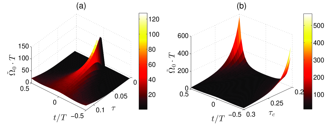
Figure 1: (a) The relationship between the dimensionless parameter $T\tilde{\Omega}_{0}$ and $\tau$. The maximum value for $T\tilde{\Omega}_{0}$ is when $t=0$, and $T\tilde{\Omega}_{0}^{max}$ observably decreases with the increasing of $\tau$ as shown in the figure. (b) The relationship between the dimensionless parameter $T\tilde{\Omega}_{0}$ and $\tau_{c}$. The maximum value for $T\tilde{\Omega}_{0}$ is when $t=\pm T/2$, and $T\tilde{\Omega}_{0}^{max}$ also decreases with the increasing of $\tau_{c}$ as shown in the figure. We choose $\tau_{c}=0.3T$ and $\tau=0.12T$ in plotting Figs. 1 (a) and (b), respectively. Other parameters are $\gamma_{0}=0.1$ and $\varphi=\pi/5$.

In order to design a reference process to obtain the target state $|3\rangle$ from the initial state $|1\rangle$ through the evolution path $|\tilde{\phi}_{0}(t)\rangle$, we can accordingly set the boundary condition as $\theta(t_{i})=0,\ \theta(t_{f})=\pi/2$ and $\gamma(t_{i})=\gamma(t_{f})=0$. Therefore, we consider the optimal STIRAP pulses discussed in Ref. Pra80013417 ,

$$\Omega_{0}=\chi e^{-(t/T_{0})^{2n}},\ \theta=\frac{\pi}{2(1+e^{-t/\tau})},$$ (80)

with $\chi$ being the peak of the pulses. To satisfy the boundaries $\theta(t_{i})=0$ and $\theta(t_{f})=\pi/2$, $\tau$ should satisfies $0<\tau\leq 0.12T$ ($T=t_{f}-t_{i}$ is the total operation time and $\theta(t_{i})\approx 0.07\pi$ when $\tau=0.12T$). For the angle $\gamma$, the boundaries are $\gamma(t_{i})=\gamma(t_{f})=0$ and $\dot{\gamma}(t_{i})=\dot{\gamma}(t_{f})=0$ to simulate the modified pulses with a finite duration. The simplest choice for $\gamma$ can be Gaussian function that

$$\gamma=\pi\gamma_{0}\cdot\exp(-t^{2}/\tau_{c}^{2}),$$ (81)

with $0<\gamma_{0}<0.5$ and $0.2T<\tau_{c}<0.3T$. Then we have

$$\dot{\theta}=\frac{\pi}{2}\cdot\frac{e^{-t/\tau}}{\tau(1+e^{-t/\tau})^{2}},\ \dot{\gamma}=-\frac{2\pi\gamma_{0}t}{\tau_{c}^{2}}e^{-t^{2}/\tau_{c}^{2}}.$$ (82)

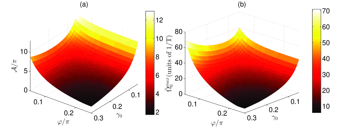
Figure 2: (a) The total pulse area $\mathcal{A}$ given by Eqs. (73) and (84) versus the parameters $\gamma_{0}$ and $\varphi$. (b) $T\tilde{\Omega}_{0}^{max}$ versus the parameters $\gamma_{0}$ and $\varphi$, where $\tilde{\Omega}_{0}^{max}$ means the maximal value for the modified pulse amplitude $\tilde{\Omega}_{0}$. Other parameters are $\tau=0.115T$ and $\tau_{c}=0.3T$.

To analyze total interaction time for a scheme, in general, the dimensionless parameter $T\tilde{\Omega}_{0}^{max}$ ($\tilde{\Omega}_{0}^{max}$ is the maximum value of $\tilde{\Omega}_{0}$) is a common measurement scale. Beware that $\tilde{\Omega}_{0}^{max}$ is usually a little larger than the maximum value for $\tilde{\Omega}_{p,(s)}(t)$, the total interaction time measured by the $T\tilde{\Omega}_{0}^{max}$ is in fact a little larger than the real one. While, $T\tilde{\Omega}_{0}^{max}$ would help a lot for quantitative analysis in the total interaction time, so, we tend to use $T\tilde{\Omega}_{0}^{max}$ as a measurement scale for the total interaction time in the following discussion. Then, with ${\theta}$ and ${\gamma}$ given in Eqs. (80) and (81), we find, within the selectable range for the parameters, $T\tilde{\Omega}_{0}^{max}$ is in inverse proportion to $\tau$ and $\tau_{c}$. Numerical simulation as shown in Fig. 1 which displays the relationship between $T\tilde{\Omega}_{0}$ and $\tau$ [see Fig. 1 (a)], the relationship between $T\tilde{\Omega}_{0}$ and $\tau_{c}$ [see Fig. 1 (b)], also verifies this point. That is, $\tau$ and $\tau_{c}$ should be chosen the larger the better to shorten the interaction time. Therefore, we might choose the largest $\tau=0.115T$ and $\tau_{c}=0.3T$ for the preliminary discussion of the approach. To analyze the energy cost of the process, we define the total pulse area for the process as

$$\mathcal{A}=\int_{-\infty}^{+\infty}dt\sqrt{\tilde{\Omega}_{p}^{2}(t)+\tilde{\Omega}_{s}^{2}(t)}.$$ (83)

For the pulses in Eq. (73), the total pulse area is

$$\mathcal{A}=\int_{-\infty}^{+\infty}dt\tilde{\Omega}_{0}(t).$$ (84)

Fig. 2 (a) shows the total pulse area $\mathcal{A}$ versus $\gamma_{0}$ and $\varphi$. As we can find, more energy should be cost with both the decreasing of $\varphi$ (corresponding to the increasing of the detuning) and the decreasing of $\gamma_{0}$ (corresponding to the decreasing of the excited-state population) as shown in the figure. In Fig. 2 (b), we plot the dimensionless parameter $T\tilde{\Omega}_{0}^{max}$ versus $\gamma_{0}$ and $\varphi$. Obviously, the total interaction time increases with the increasing of detuning as shown in Fig. 2 (b). The deviation from the complete population transfer displayed in Fig. 3 (the upper frame) with a logarithmic scale shows the high efficiency for the present approach. We obtain the transfer with an accuracy to about four digits for areas are: (i) $2.9\pi$ when $\varphi=\pi/4$ (the resonant case), (ii) $4.9\pi$ when $\varphi=\pi/5$ (the small detuning case), (iii) $7.9\pi$ when $\varphi=10$ (large detuning case), respectively. The corresponding total interaction time as shown in the middle frame in Fig. 3 are: (i) $T\tilde{\Omega}_{0}^{max}=11.5$ when $\mathcal{A}=2.9\pi$ for the resonant case, (ii) $T\tilde{\Omega}_{0}^{max}=19.5$ when $\mathcal{A}=4.9\pi$ for the small detuning case, (iii) $T\tilde{\Omega}_{0}^{max}=34$ when $\mathcal{A}=7.9\pi$ for the large detuning case. It is known that in the $\Lambda$-type system, the use of two successive $\pi$ pulses, respectively, for the pump and Stokes fields, or of two overlapping fields corresponds both to $\mathcal{A}=2\pi$ Aps58243 , and the minimum area in a $\Lambda$-type system for a population transfer from $|1\rangle$ to $|3\rangle$ is $\sqrt{3}\pi$ Jmp432107 . The total pulse area $\mathcal{A}$ in the present approach as shown in Figs. 2 and 3, is small enough to verify the state transfer is sped up. Then, in the lower frame in Fig. 3, we give the relationship between the parameter $\gamma_{0}$ and $\mathcal{A}$. Clearly from the figure, $\gamma_{0}$ generally decreases with the increasing of $\mathcal{A}$, which means, an increasing in the population of intermediate state is unavoidable if one wants to save energy to drive the system to the target state. This result can be understood by, the intermediate state links the whole system together just like brittle strings; the evolution of the system is interdictory without the participation of these intermediate states. By increasing the populations of intermediate states in a certain period of time, just like broadening the path for the transition between the initial state and the target state in a certain period of time, the evolution could be much faster.

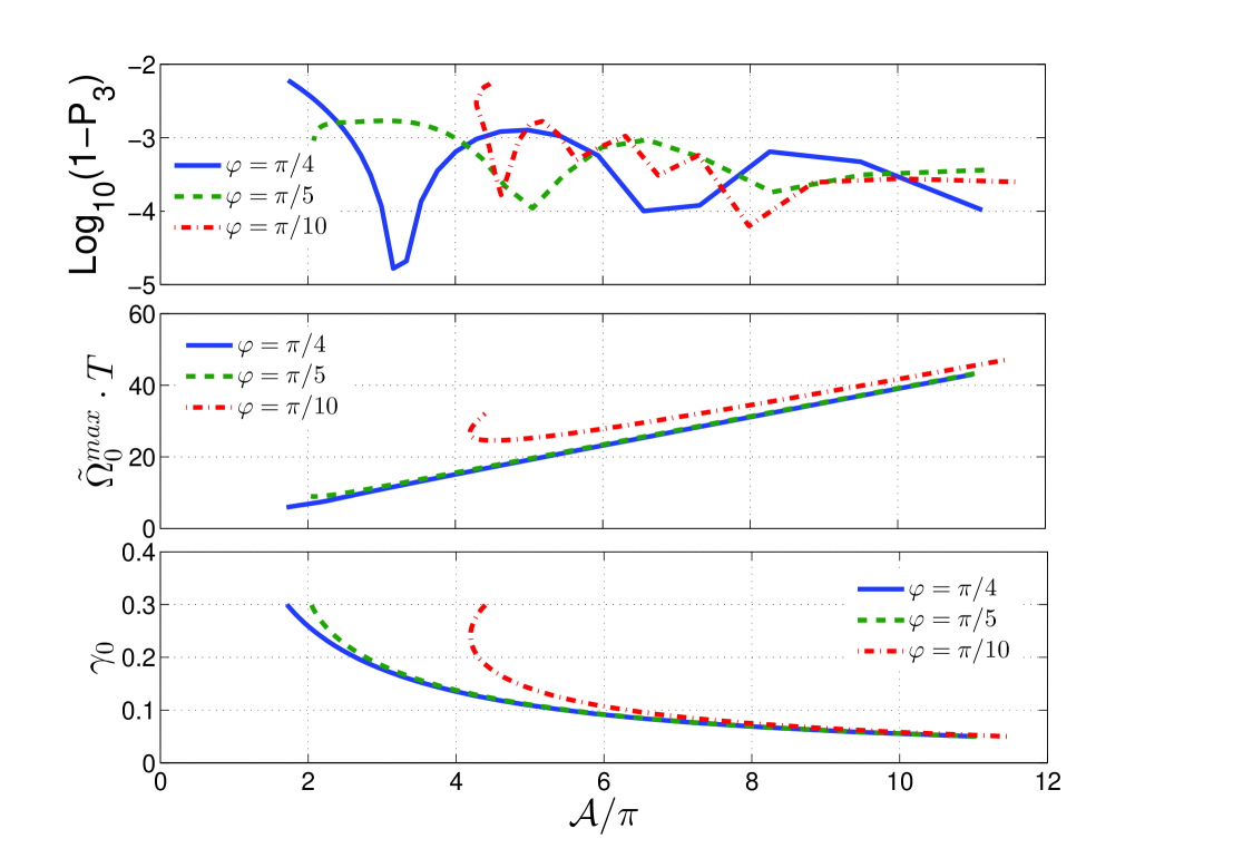
Figure 3: Upper frame: Logarithmic scale of the deviation from the complete population transfer with different choices for the parameter $\varphi$. Middle frame: The corresponding dimensionless parameter $T\tilde{\Omega}_{0}^{max}$ for the speedup process. Lower frame: The relationship between the parameter $\gamma_{0}$ (corresponding to the maximal population for the excited state $|2\rangle$) and the total pulse area $\mathcal{A}$. Other parameters are $\tau=0.115T$, $\tau_{c}=0.3T$ according to the requirement of less energy cost.

Then, with parameters $\{\gamma_{0}=0.1,\tau=0.115T,\tau_{c}=0.3T,\varphi=\pi/5\}$ (choosing $\gamma_{0}=0.1$ for a less excited-state population), we show the modified pulses $\tilde{\Omega}_{p,(s)}(t)$ and detuning $\tilde{\Delta}(t)$ in Fig. 4 (a). The maximal amplitude for the pulses in this case $\tilde{\Omega}_{0}^{max}\approx 16/T$ with pulse area $\mathcal{A}\approx 4.1\pi$. The dynamics governed by the final transitionless Hamiltonian $\tilde{H}(t)$ (with $\tau\approx 0.115T$) versus time is shown in Fig. 4 (b). For comparison, with the same parameters for the pulses and detuning, we accordingly plot the original parameters for the original Hamiltonian $H_{0}(t)$ and the time evolution of the system in Figs. 5 (a) and (b), respectively. We choose $\Omega_{0}=16/T$ in plotting Fig. 5. The total pulse area $\mathcal{A}$ corresponding to Fig. 5 is $\mathcal{A}=\int_{-\infty}^{+\infty}dt\Omega_{0}=5.09\pi$. The comparison between Fig. 4 (b) and Fig. 5 (b) shows, within a specified total evolution time $T$, the final transitionless Hamiltonian $\tilde{H}(t)$ allows a near-perfect population transfer (with $P_{3}\approx 0.997$) from $|1\rangle$ to $|3\rangle$ while the original Hamiltonian $H_{0}(t)$ fails. In fact, to satisfy the adiabatic condition $\dot{\theta}\ll|\Xi_{0}\sin^{2}{\varphi}/\cos{\varphi}|<|\Xi_{0}\cos^{2}{\varphi}/\sin{\varphi}|$ (assuming $0<\varphi<\pi/4$) for the original Hamiltonian $H_{0}(t)$, with the $\theta$ given in Eq. (80) and $\varphi=\pi/5$, $\Omega_{0}$ should be at least $30/T$ to ensure $(\Xi_{0}\sin^{2}{\varphi})/(\dot{\theta}\cos{\varphi})\geq 5$.

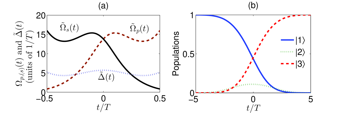
Figure 4: (a) The modified Rabi frequencies and detuning [Eq. (25)] versus time. (b) The speedup population transfer governed by the off-resonant $\Lambda$-type system with Hamiltonian $\tilde{H}(t)$. Parameters are $\tau_{c}=0.3T$, $\tau=0.115T$, $\gamma_{0}=0.1$, and $\varphi=\pi/5$. With these parameters, the maximal pulse amplitude for $\tilde{H}(t)$ is $\tilde{\Omega}_{0}^{max}\approx 16/T$.

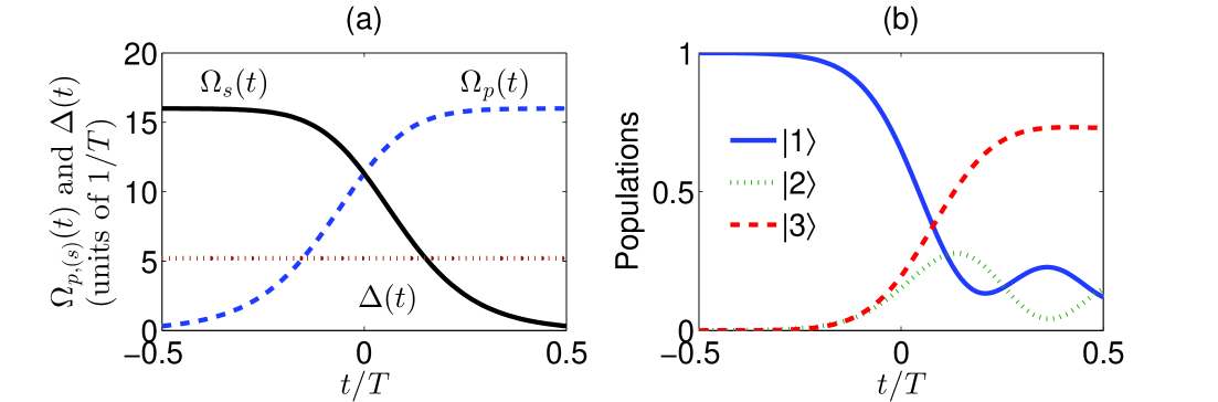
Figure 5: (a) The original Rabi frequencies and detuning [Eq. (63)] versus time. (b) The population transfer governed by the off-resonant $\Lambda$-type system with the original Hamiltonian ${H_{0}}(t)$. Parameters are $\tau_{c}=0.3T$, $\tau=0.115T$, and $\varphi=\pi/5$. The modified pulse amplitude $\tilde{\Omega}_{0}$ is in fact independent to the original pulse amplitude $\Omega_{0}$ according to Eq. (25). So, for a fair comparison, we choose a relatively larger $\Omega_{0}=16/T$ in plotting Fig. 4.

We know that the Vitanov pulses were originally derived in order to get an ultra-high and robust fidelity in an adiabatic process Pra80013417 ; Pra80043408 . To check the robustness against noise after the correction to the pulses, we define a parameter with noise as

$${G}_{F}=G+G\cdot\varpi,$$ (85)

where $G=\tilde{\Omega}_{0},\ \tilde{\theta},\ \tilde{\Delta}(t)$, and $-0.1<\varpi<0.1$ is a random number. This allows one to model instantaneous fluctuations of the detunings and of the pulse shapes. We can find from Fig. 6 (a) that when such a noise is considered, the shapes for $\tilde{\Omega}_{p,(s)}$ and $\tilde{\Delta}(t)$ have been destroyed seriously. However, a nearly perfect population transfer (with the final population for $|3\rangle$ is $P_{3}(t_{f})\approx 0.993$) still can be achieved as shown in Fig. 6 (b). Which means the present approach with modified Vitanov pulses is still robust against instantaneous fluctuations on the parameters. The main decoherence effect in the population transfer is due to the spontaneous emission from the excited state $|2\rangle$. The total spontaneous emission from the excited state, is generally decided by two factors: the total interaction time and the average population of the excited state. According to Eq. (46), the population for the excited state $|2\rangle$ is $P_{2}=\sin^{2}{\gamma}$. The average population of the excited state is thus given as

$$\overline{P}_{2}=\frac{1}{\gamma_{max}-\gamma_{min}}\int_{\gamma_{min}}^{\gamma_{max}}\sin^{2}{\gamma}d\gamma,$$ (86)

where $\gamma_{max}$ is the maximum value and $\gamma_{min}$ is the minimum value for $\gamma$, respectively. With $\gamma$ given inform of Eq. (81), we have $\gamma_{max}=\gamma_{0}\pi$, $\gamma_{min}=0$, and

$$\overline{P}_{2}=\frac{1}{2}-\frac{\sin(2\gamma_{0}\pi)}{4\gamma_{0}\pi}.$$ (87)

We use a function $\epsilon=\Gamma_{a}\cdot\overline{P}_{2}\cdot(T\tilde{\Omega}_{0}^{max})$ ($\Gamma_{a}$ can be regarded as the average loss rate of the excited state which relates to the spontaneous emission) to describe the probability of loss of the excited state. Beware that $\epsilon$ is not limited by 1, so, in general, we can not directly treat it as the fidelity error caused by spontaneous emission. When $\tau=0.115T$ and $\tau_{c}=0.3T$, we find

$$\tilde{\Omega}_{0}^{max}=\tilde{\Omega}_{0}|_{t=0}=\frac{\pi}{\tau}\sqrt{\cot^{2}{(\pi\gamma_{0})}+\frac{4\cot^{2}{2\varphi}}{\cos^{2}(\pi\gamma_{0})}}.$$ (88)

According to Eqs. (87) and (88), we have $\frac{\partial}{\partial\varphi}\epsilon<0$ ($0<\varphi<\pi/4$) and $\frac{\partial}{\partial\gamma_{0}}\epsilon<0$ ($0.05<\gamma_{0}<0.3$). $\epsilon$ is in inverse proportion to both $\gamma_{0}$ and $\varphi$. Fig. 7 which shows $\epsilon$ versus $\gamma_{0}$ and $\varphi$ also verifies this point. This result means, a large $\gamma_{0}$ which significantly shortens the interaction time and reduces the total pulse area, however, fails to restrain the influence of spontaneous emission. This is because when the interaction time is short enough, further reducing the interaction time can not counteract the negative effect caused by the excited-state population $P_{2}$. When the interaction time is short enough, reducing the excited-state population is more important to restrain the influence of spontaneous emission. One of the effective ways to reduce the excited-state population, as we know, is increasing the detuning. Nevertheless, increasing the detuning will inevitably increase the total interaction time. This is why a large detuning also fails to restrain the influence of spontaneous emission as shown in Fig. 7. Therefore, taking the requirements of short interaction time, less energy cost, and robustness against spontaneous emission all into account, an off-resonant system with small detuning might the best choice to realize the speedup STIRAP in practice. In the following, we would like to numerically show the influence of spontaneous emission on the fidelity of population transfer under Markov approximation with Lindblad equation Cmp48119

$$\frac{d\rho}{dt}=\frac{1}{i\hbar}[\tilde{H},\rho]+\sum_{n=1,3}{\Gamma_{n}}[S_{n}^{-}\rho S_{n}^{+}-\frac{1}{2}(S_{n}^{+}S_{n}^{-}\rho+\rho S_{n}^{+}S_{n}^{-})],$$ (89)

where $\rho$ is the density matrix, $S_{n}^{-}=|n\rangle\langle 2|$, and $S_{n}^{+}=(S_{n}^{-})^{{\dagger}}$ are the so-called Lindblad operators, $\Gamma_{n}$ is the spontaneous emission rate from the excited state $|2\rangle$ to the ground state $|n\rangle$. We plot the fidelity of the population transfer with considering the small detuning case (choosing $\varphi=\pi/5$) versus $\Gamma_{n}$ in Fig. 8. The spontaneous emission from the excited state $|2\rangle$ to the ground state $|1\rangle$ affects the fidelity more seriously than that to the ground state $|3\rangle$ as shown in the figure. According to the result, we verify that the population transfer is robust against spontaneous emission since it is still about $85\%$ even when $\Gamma_{1}=\Gamma_{3}=0.5\tilde{\Omega}_{0}^{max}$. Here we can find an interesting phenomenon from the figure that when $\Gamma_{1}$ is relatively large ($\Gamma_{1}>0.2\Omega_{0}^{max}$), spontaneous emission from the excited state $|2\rangle$ to the ground state $|3\rangle$ becomes a favourable factor in obtaining a high fidelity of the scheme. The reason behind this phenomenon is because the state $|3\rangle$ is just the target state, so spontaneous emission from the excited state $|2\rangle$ to the ground state $|3\rangle$ indeed increases the fidelity.

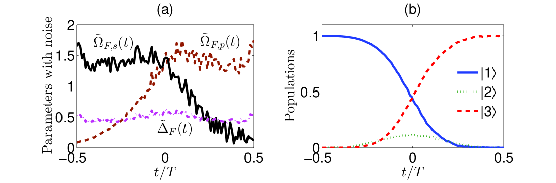
Figure 6: (a) The shapes for the modified pulses and detuning when instantaneous fluctuations are taken into consideration according to Eq. (85). (b) The population transfer with the fluctuation-included parameters. Shown in the figure, even when the shapes for the modified pulses and detuning are destroyed seriously, a nearly perfect population transfer (with $P_{3}\approx 0.993$) still can be achieved. Which verifies that the scheme is robust against the instantaneous fluctuations on the parameters.

Our scheme can be realized with the setup of Ref. arxiv1607 , where a solid-state $\Lambda$ system is hosted by a single nitrogen-vacancy centre in diamond at low temperature, and the shapes and phases of the driving pulses can be modulated by electrooptic modulators. With a single tunable laser (637.2nm), the maximal amplitude of the modified pulses can be chosen as $\tilde{\Omega}_{0}=2\pi\times 171$MHz (under the RWA), the corresponding operation time is $T\approx 14$ns which is smaller than the life time for the $|A_{2}\rangle=|2\rangle$ spin-orbit excited state at temperature $5.5$K. This result is very close to that in Ref. arxiv1607 with resonant driving system, and it is much better than that (maximal amplitude of the modified pulses is $\tilde{\Omega}_{0}\approx 6\times 2\pi$MHz and operation time $T=0.4$ms) in Ref. Natc712479 with highly detuned pulses. Ref. arxiv1607 also reports the relaxation rates $\Gamma_{1}/2\pi=4.3$MHz and $\Gamma_{3}/2\pi=8.5$MHz for decay of the excited $|A_{2}\rangle$ level into the $|1\rangle$ and $|3\rangle$ ground states, respectively. With the experimental data, we can find the fidelity of the population transfer is $97.48\%$.

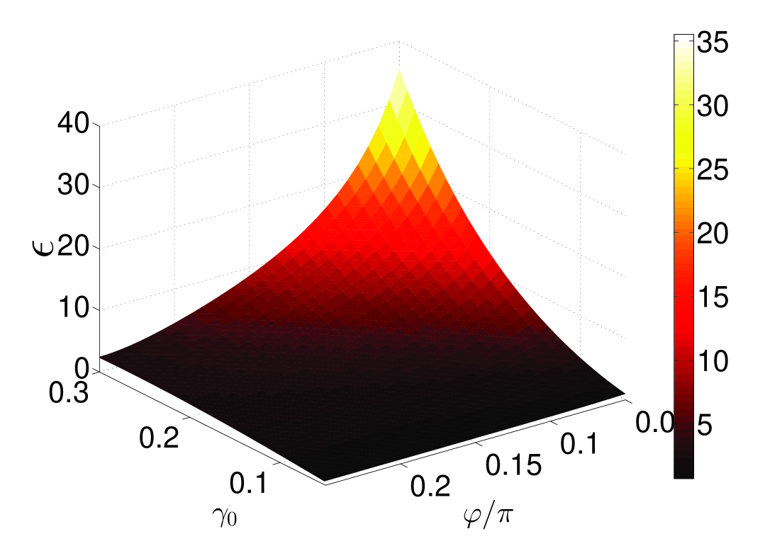
Figure 7: The measurement scale $\epsilon$ defined by $\epsilon=\Gamma_{a}\cdot\overline{P}_{2}\cdot(\tilde{\Omega}_{0}^{max}\cdot T)$ for analyzing the influence of spontaneous emission versus $\gamma_{0}$ and $\varphi$. Parameters are chosen as $\tau=0.115T$, $\tau_{c}=0.3T$, and $\Gamma_{a}=0.5$ in plotting the figure. For a robust process, $\epsilon$ is the smaller the better, so a very large $\gamma_{0}$ which though significantly shortens the interaction time, and a very small $\varphi$ which though restrains the excited-state population, are certainly both not desirable.

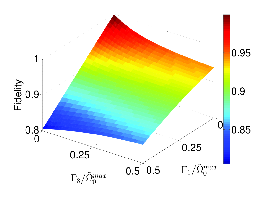
Figure 8: The fidelity defined by $|\langle 3|\rho(t_{f})|3\rangle|^{2}$ for the population transfer versus $\Gamma_{1}$ and $\Gamma_{3}$ in an off-resonant system with small detuning. Parameters are chosen as $\tau=0.115T$, $\tau_{c}=0.3T$, $\gamma_{0}=0.1$, and $\varphi=\pi/5$. In this case, the interaction time $T\approx 16/\tilde{\Omega}_{0}^{max}$, the total pulse area $\mathcal{A}\approx 4.1\pi$.

V Conclusion

We have shown that the intermediate Hamiltonian could be directly designed by using the original Hamiltonian and the CD Hamiltonian. With the help of the easy-to-get intermediate Hamiltonian, we have presented a general approach to remove the adiabatic condition to speed up the corresponding population transfer process without adding the traditional CD Hamiltonian. Our method is significantly different from that of Ref. Prl116230503 , where the important intermediate Hamiltonian is constructed with some specified dressed states. The present approach is physically transparent and extremely flexible. We further show with the help of the intermediate Hamiltonian, speedup scheme can be realized even without breaking down the structure of the original Hamiltonian, which is important in view of experiment.

Further applications or extensions of this approach could be in fields such as shortcuts to non-Hermitian quantum adiabatic computation Pra84023415 ; Pra93052109 ; Pra8705250289063412 , dissipative master equations Pra78033417 ; Njp16053017 , or more complicated systems Pra94043623 ; Njp18012001 ; Pra95022332 .

This work was supported by the National Natural Science Foundation of China under Grants No. 11575045, No. 11374054 and No. 11675046.

References

(1) T. W. Hänsch,
Rev. Mod. Phys.
78, 1297 (2006).
(2) P. Král, I. Thanopulos, and M. Shapiro,
Rev. Mod. Phys.
79, 53 (2007).
(3) J. Stolze and D. Suter, Quantum Computing: A Short Course from Theory to Experiment, 2nd ed. (Wiley-VCH, Berlin, 2008).
(4) S. B. Zheng,
Phys. Rev. Lett
95, 080502 (2005).
(5) X. Chen, I. Lizuain, A. Ruschhaupt, D. Guéry-Odelin, and J. G. Muga,
Phys. Rev. Lett.
105, 123003 (2010).
(6) E. Torrontegui, S. Ibáñez, S. Martínez-Garaot, M. Modugno, A. del Campo, D. Gué-Odelin, A. Ruschhaupt,
X. Chen, and J. G. Muga,
Adv. Atom. Mol. Opt. Phys.
62, 117 (2013).
(7) A. del Campo,
Phys. Rev. Lett.
111, 100502 (2013).
(8) S. Ibáñez, X. Chen, E. Torrontegui, J. G. Muga, and A. Ruschhaupt,
Phys. Rev. Lett.
109, 100403 (2012).
(9) M. Demirplak and S. A. Rice,
J. Phys. Chem. A
107, 9937 (2003);
J. Chem. Phys.
129, 154111 (2008).
(10) M. V. Berry,
J. Phys. A
42, 365303 (2009).
(11) R. G. Unanyan, L. P Yatsenko, K. Bergmann, B. W. Shore,
Opt. Commun.
139, 48 (1997).
(12) A. del Campo and K. Sengupta,
Eur. Phys. J. Special Topics
224, 189 (2015).
(13) J. F. Schaff, X. L. Song, P. Vignolo, and G. Labeyrie,
Phys. Rev. A
82, 033430 (2010).
(14) J. F. Schaff, X. L. Song, P. Capuzzi, P. Vignolo, and G. Labeyrie,
Eur. Phys. Lett.
93, 23001 (2011).
(15) X. Chen and J. G. Muga,
Phys. Rev. A
86, 033405 (2012).
(16) S. Martínez-Garaot, E. Torrontegui, X. Chen, and J. G. Muga,
Phys. Rev. A
89, 053408 (2014).
(17) E. Torrontegui, S. Martínez-Garaot, and J. G. Muga,
Phys. Rev. A
89, 043408 (2014).
(18) J. G. Muga, X. Chen, S. Ibáñez, I. Lizuain, and A. Ruschhaupt,
J. Phys. B
43, 085509 (2010).
(19) A. del Campo,
Phys. Rev. A
84, 031606(R) (2011);
Eur. Phys. Lett.
96, 60005 (2011).
(20) T. Opatrný and K. Mølmer,
New J. Phys.
16, 015025 (2014).
(21) S. An, D. Lv, A. del Campo, and K. Kim, Nature
Commun. 7, 12999 (2016).
(22) A. Baksic, H. Ribeiro, and A. A. Clerk,
Phys. Rev. Lett.
116, 230503 (2016).
(23) Y. X. Du, Z. T. Liang, Y. C. Li, X. X. Yue, Q. X. Lv, W. Huang, X. Chen, H. Yan, and S. L. Zhu, Nature Commun.
7, 12479 (2016).
(24) X. K. Song, Q. Ai, J. Qiu, and F. G. Deng,
Phys. Rev. A
93, 052324 (2016).
(25) G. Vasilev, A. Kuhn, and N. Vitanov,
Phys. Rev. A
80, 013417 (2009).
(26) B. W. Shore, The Theory of Coherent Atomic Excitation
(Wiley, New York, 1990);
Acta Phys. Slov.
58, 243 (2008).
(27) U. Boscain, G. Charlot, J.-P. Gauthier, S. Guérin, and H. R. Jauslin,
J. Math. Phys.
43, 2107 (2002).
(28) G. Dridi, S. Guérin, V. Hakobyan, H. R. Jauslin, and H. Eleuch,
Phys. Rev. A
80, 043408 (2009).
(29) G. Lindblad,
Commun. Math. Phys.
48, 119 (1976).
(30) B. B. Zhou, A. Baksic, H. Ribeiro, C. G. Yale, F. J. Heremans, P. C. Jerger, A. Auer, G. Burkard, A. A. Clerk, and D. D. Awschalom,
arXiv:1607.06503 (2016) (has been acceptted by Nature Physics).
(31) S. Ibáñez, S. Martínez-Garaot, X. Chen, E. Torrontegui, and J. G. Muga,
Phys. Rev. A
84, 023415 (2011).
(32) Y. H. Chen, Y. Xia, Q. C. Wu, B. H. Huang, and J. Song,
Phys. Rev. A
93, 052109 (2016).
(33) B. T. Torosov, G. Della Valle, and S. Longhi,
Phys. Rev. A
87, 052502 (2013);
89, 063412 (2014).
(34) X. Lacour, S. Guérin, and H. R. Jauslin,
Phys. Rev.A
78, 033417 (2008).
(35) G. Vacanti, R. Fazio, S. Montangero, G. M. Palma, M. Paternostro, and V. Vedral,
New J. Phys.
16, 053017 (2014).
(36) A. Sala, D. L. Núñez, J. Martorell,L. D. Sarlo, T. Zibold, F. Gerbier, A. Polls, and B. Juliá-Díaz,
Phys. Rev. A
94, 043623 (2016).
(37) S. Deffner,
New J. Phys.
18, 012001 (2016).
(38) X. K. Song, F. G. Deng, L. Lamata, and J. G. Muga,
Phys. Rev. A
95, 022332 (2017).