An Open-Data Analysis of Heterogeneities in Lung Cancer Premature Mortality Rate and Associated Factors among Toronto Neighborhoods

Abstract

In public health, various data are rigorously collected and published with open access. These data reflect the environmental and non-environmental characteristics of heterogeneous neighborhoods in cities. In the present study, we aimed to study the relations between these data and disease risks in heterogeneous neighborhoods. A flexible framework was developed to determine the key factors correlated with diseases and find the most relevant combination of factors to explain observations of diseases through nonlinear analyses. Taking Lung Cancer Premature Mortality Rate (LCPMR) in Toronto as an example, two environmental factors (green space, and industrial pollution) and two non-environmental factors (immigrants, and mental health visits) were identified in the relational analysis of all of the target neighborhoods. To determine the influence of the heterogeneity of the neighborhoods, they were clustered into three different classes. In the most severe class, two additional factors related to dwellings were determined to be involved, which increased the observation’s deviance from 48.1% to 80%. The factors determined in this study may assist governments in improving public health policies.

 

 

INTRODUCTION

Public health researchers have shown that many diseases are correlated with geographic variations among the neighborhoods of cities. Moreover, the correlations between health and neighborhood/area characteristics and independent of population-level attributes diez2001investigating ; macintyre2002place . For instance, in Boston, the incidence of diabetes is correlated with ethnic disparities between different neighborhoods piccolo2015role . In Phoenix, air pollution contributes to disparities in the incidence of asthma among children of different areas grineski2007incorporating . In New York, environmental factors contribute to the spatial disparities of asthma incidence corburn2006urban . Lung cancer mortality was reported having a positive association with ambient nitrogen dioxide villeneuve2013cohort .

Therefore, it is important to explore the factors that influence the occurrence of different diseases in the neighborhoods of cities. The determination of these factors would provide valuable insights into disease risk factors, and guide governments’ actions in reducing harmful materials in human environments. For example, the Canadian government is currently in the process of banning asbestos because of asbestos-related diseases, such as lung cancer cbc_ban2016 .

The determination of disease risk factors requires numerous kinds of public-health-related data for many cities. Some of these data are rigorously collected and published with open access by government departments. For example, in New York, the Open Data Plan makes public data (such as business, education, and dwelling data) generated by various New York City agencies and organizations available for public use NYCopenData2016 . In Toronto, the available open data are rich and organized into 15 categories (such as culture, finance, and health) TorontoOpendata2016 . The industrial records date back to 1995 NPRI1995 . Rich open data are valuable, and their availability encourages future research to maximize their benefit to society. Based on these open data, we investigated how geographic factors influence diseases in the neighborhoods of cities.

In the present study, we used lung cancer as a case study. Although the premature mortality rates of lung cancer have decreased slowly since the late 1990s howlader2011seer , it remains the most common cause of cancer-related death in men and the second most common in women (after breast cancer) stewart2014world ; jemal2011global ; ferlay2010estimates , especially in large cities hunt2015black . For example, worldwide, lung cancer is one of 5 most common causes of cancer death, accounting for 1.69 million deaths in 2015 WHO2017 . In large cities, such as Toronto, lung cancer is one of the most common cancers and the leading cause of cancer deaths, especially in the low-income groups TPHLC2008 ; TPHLC2015 . The spatial distribution of the Lung Cancer Premature Mortality Rate (LCPMR) in the 140 neighborhoods of Toronto is depicted in Fig.1.

Figure 1: LCPMR per 100,000 persons in 138 out of the 140 neighborhoods of Toronto (2003–2007) ASD2006 (where the data from two neighborhoods were missing). The spatial map was created using OpenStreetMap online platform (http://http://www.openstreetmap.org/) ($\copyright$ OpenStreetMap contributors) under the license of CC BY-SA (http://www.openstreetmap.org/copyright). More details of the licence can be found at http://creativecommons.org/licenses/by-sa/2.0/. Line graphs were drawn using Tableau Software for Desktop version 9.2.15 (https://www.tableau.com/zh-cn/support/releases/9.2.15).

Lung cancer has been widely studied with respect to its correlation with a variety of closely related factors, such as population lifestyle hystad2014geographic , natural environment crouse2015within , built environment jackson2013health , and social environment berglund2012social ; casper2001definition ). Additionally, other indicators that reflect some degree of susceptibility to lung cancer have also been studied, such as socioeconomic status dominguez2015lung ; qi2006determinants , ethnicity jack2011lung ; qi2006determinants , and physical activity brenner2016leisure ; emaus2010physical ; mao2003physical . Moreover, residents’ lifestyle and work histories have been considered because of the long-term process of lung cancer development tomczak2016long ; Lung2016 ; tomczak2016long .

Regions and neighborhoods in urban areas generally exhibit geographic variations in various factors heterogeneous2011 ; york2011ethnic ; hystad2014geographic . For example, Toronto consists of many neighborhoods with heterogeneous environments, which exhibit variations in LCMPR TorontoCHPP2016 , lifestyle TorontoHSI2016 , demographic factors TorontoCHPP2016 ; TorontoCP2006 ; TorontoN2011 , and industry TorontoChem2012 . Hence, in the present study, we focused on the relations between LCMPR and heterogeneous geographic factors, based on open data from the neighborhoods of Toronto.

Most studies of lung cancer epidemiology have focused on the relations between various factors and lung cancer. Broadly speaking, two kinds of related factors, environmental and non-environmental, have been studied. Environmental factors consist of those present where a person grows, lives, works, and ages ruiz2016contributions . Substances in the natural, built, and social environments may have direct interactions with the body and thereby induce kinds of diseases Protection2016 . The natural environment denotes naturally occurring factors, such as water, air, minerals, and climate ruiz2016contributions . For example, LCPMR is related to exposure to radon and asbestos Asbestos2016 ; lubin1995lung . Furthermore, air pollutants can increase the oxidative stress in cells and elevated lung cancer risk yang2015spatial . The built environment refers to the manmade surroundings that provide the settings for human activity ruiz2016contributions . For example, green space has a negative correlation with lung cancer mortality mitchell2008effect . The social environment encompasses social interactions and demographic factors such as dwellings and food security ruiz2016contributions . For example, mental health has a potential correlation with LCMPR pirl2012depression .

Non-environmental factors, such as lifestyle factors (for example, smoking and physical activity) hystad2014geographic , ethnicity, and immigration brown2016detailed , may correlate with disease outcomes. For example, physical activity shows a protective effect on lung cancer risk, with a validated biological mechanism brenner2016leisure ; emaus2010physical ; mao2003physical . To determine the correlation of these factors with lung cancer, they are commonly modeled as linear relations using regression analyses, such as linear regression argo2010chronic and logistic regression lopez2013lung .

Research has mainly considered a small number of factors in correlation analyses. They are meaningful, but may overlook other closely related factors. Therefore, it is necessary to conduct analyses of large open datasets to determine the correlation of a large group of factors with LCMPR. Additionally, studies have mainly conducted city-level case studies. However, the heterogeneity of neighborhoods is important, as the development of neighborhoods and communities is vital to improve public health syme2009importance .

In the present study, we investigated how various factors influence LCPMR in the neighborhoods of a city, based on environmental and non-environmental factors from open data, especially in neighborhoods with disproportionately high LCPMR. Specifically, we used the city of Toronto as a case study, which has a relatively high LCPMR LC2010 . Its neighborhoods are characterized by variations in LCPMR, and related factors (such as lifestyles ASD2006 and built environment TorontoN2011 ).

We analyzed the relations between various factors and LCPMR using the generalize additive model (GAM) hastie1990generalized ; wood2006generalized . GAM was used to model the nonlinearity of the relations in all of the neighborhoods. GAM is a non-parametric regression method that is well suited to studying the relations between various factors wood2006generalized . To explore the influence of the heterogeneity of neighborhoods, we further explored specific neighborhoods using the same method.

We identified neighborhoods with significant lung cancer factors based on open data. After dimension reduction using principal component analysis (PCA) (which has been widely used for such a purpose in various fields such as neuroscience brenner2000adaptive ), these factors were used as indicators for clustering neighborhoods. A model-based clustering method was used to cluster the neighborhoods. The data are assumed to follow a distribution that is the mixture of two or more components, which are modeled by Gaussian distributions. This method is statistically more robust than clustering algorithms based on geometric procedures (such as the k-means algorithm and hierarchical clustering algorithms) bouveyron2014model . After clustering, we analyzed these factors using GAM.

Numerous kinds of rigorously produced and published open data for Toronto are related to lung cancer. To sufficiently describe each neighborhood of Toronto, we collected environmental and non-environmental factors from open data. For example, many environmental factors (such as soil radon potential and green space) could be found in the open demographic census TorontoCHPP2016 ; TorontoCP2006 ; TorontoN2011 . In addition to commonly used factors such as green space and soil radon potential, to investigate the influence of dwellings on LCPMR, we chose the percentage of dwellings constructed before 1990, as during that period it was common to use asbestos for the insulation of dwellings in Toronto. Moreover, to study the influence of industry, we considered the air pollution originating from factories that no longer existed. As lung cancer may remain dormant for around 20 years de2014spatial , it is therefore common to choose a period of 20 years before the study tomczak2016long . Hence, we used data regarding the industrial distribution in Toronto 20 years ago TorontoChem2012 ), preprocessed by examining the effects of air pollution risks and the wind (which influences the air pollution range). Data related to many non-environmental factors can be found in the open health surveillance indicators TorontoHSI2016 , including income, university attendance, mental health, and immigration status, to determine population lifestyles.

We first analyzed all of the neighborhoods in Toronto to determine the general relations between the target factors and LCPMR using GAM. Two environmental factors (green space and industrial pollution) were derived from a combination of four factors that exhibited the highest deviance (48.1%) among all of the neighborhoods. Along with an additional two non-environmental factors (immigrants and mental health visits), these factors were found to show the most significant explanatory ability of the 11 significant lung-cancer-relevant factors. However, the deviance explained by GAM was insufficient, possibly because the heterogeneity of the neighborhoods was not considered. Therefore, we clustered neighborhoods using the model-based clustering method. The neighborhoods were clustered into three classes by using the model-based clustering method with the best value of Bayesian Information Criterion (BIC) as a statistical measure to determine unknown parameters (such as the appropriate total number of classes). Class A corresponded to low LCMPR neighborhoods. Classes B and C both exhibited high LCPMR, but were featured by different levels of demographic factors. For example, the average value of median income over neighborhoods in class B was $74,495, much higher than that in class C ($44,582). We chose to focus on investigating the two high-LCPMR classes, especially class C, which included enough neighborhoods for further group analysis. For classes B and C, we qualitatively and quantitatively evaluated the relations between relevant factors and LCPMR. In view that there were only 11 neighborhoods involved in class B, we focused on the single-factor analysis to find its factor (percentage of dwellings constructed before 1990) with the highest explanatory ability (66%) observed. While there were 58 neighborhoods in class C, multi-factor analysis can be applied. In addition to the four most significant factors identified in the analysis of all of the neighborhoods, two dwelling factors (percentage of dwellings requiring major repairs and percentage of dwellings constructed before 1990) were also included in the group with the highest explanatory ability (80%) observed for class C. Compared with the analysis of all of the neighborhoods, the deviance was better explained in specific neighborhoods. Specifically, more dwelling-related factors were incorporated, which increased the deviance explained from 48.1% to 80%.

Based on public health related open data, we studied the factors influencing LCPMR in all of the neighborhoods. Then, to investigate the heterogeneity of the neighborhoods, we focused on factors affecting specific neighborhoods. A flexible framework was used to estimate the correlation of various factors with LCPMR, and determine which group of factors exhibited the best explanation. Clustering of neighborhoods was performed to determine their heterogeneity. Overall, 12 factors were found to be significantly correlated with LCPMR. LCPMR was best explained by a group of four factors (immigrants, mental health visits, industrial pollution, and green space). When limiting the analysis to a class of high-risk neighborhoods, the LCPMR was best explained by incorporating two additional dwelling-related factors. This research may be used to develop government guidelines for future public health policies and contribute to balancing housing, industry, and health priorities. For example, based on the industrial and dwelling factors, neighborhoods containing a large proportion of old houses should be prioritized, especially where industrial factories are also significant. The analysis of mental health and green space may also support the prioritization of civic culture. Although a specific disease and location were studied in this work, the methods used and questions raised in this work are broadly applicable and may motivate similar public health research.

DATA

To conduct our study of Toronto, we collected data regarding a variety of factors (as shown in Tab. 1) related to LCMPR from diverse open data sources. Specifically, the LCMPR, the environmental factor of green space, and some non-environmental lifestyle factors (such as mental health visits, immigration status, income and university attendance) were obtained from Toronto Community Health Profiles (2006–2013) TorontoLCPMR2007 ; Urban2013 ; AHD2012 ; ASD2006 . For more details, LCMPR denotes the lung cancer premature mortality rate, as the premature deaths per 100,000 persons due to lung cancer TorontoLCPMR2007 . The factor of mental health visits denotes the percentage of people who visit the mental health service AHD2012 . As for the green space data, it refers to the average amount of green space per km² in a 1-km diameter circular region Urban2013 . And, the factors of median income, immigrants and university attendance rate represent the percentages of immigrants, households with median income and population with a university degree in a neighborhood, respectively ASD2006 . There were also some non-environmental lifestyle factors (such as fruit consumption, smoking habits, and physical activities), which were obtained from Toronto’s Health Indicator Series (2007–2012) IS2012 ; Smoking2007 ; PA2010 . Specifically, the factors of fruit consumption, smoking rate, and physical activity rate denote the percentages of people who consume enough daily vegetables and fruits IS2012 , smoke Smoking2007 , and have moderately active levels of physical activities PA2010 , respectively. Other non-environmental factors (such as age) were obtained from Canada Statistics in 2006 TorontoCP2006 . Specifically, the factors of three age groups from 30 to 74 refer to their populations over neighborhoods TorontoCP2006 .

Data regarding environmental factors were related to the types of dwellings as obtained from the National Household Survey (2011) TorontoN2011 . For example, the factors of dwellings requiring major repairs and dwellings constructed before 1990 denote the percentages of dwellings in need of major repairs and built before 1990, respectively TorontoN2011 . And the natural environment factor of soil radon potential is to measure risk from soil radon from the study in 2008 chen2008variation .

We incorporated industrial influences into our study. However, most industrial facilities that were present in Toronto have recently moved elsewhere. As lung cancer can remain dormant for up to 20 years de2014spatial , we used data aggregated from industrial records from 1995 and 2012 (around 20 years before the target year of 2006). Although we lacked data from 2006, the aggregated data represented the general industrial environment of Toronto before 2006.

Industrial pollution can be spread from a pollution source by wind. Therefore, to calculate the industrial pollution, wind effects are needed to be considered. The wind analysis process is detailed in the Methods section. To estimate the potential risk of industrial pollution, we obtained the toxic equivalency potentials (TEP) for relevant pollutants from the ChemTRAC Annual Report TorontoChem2012 .

Data regarding 16 factors were collected from open data sources, as mapped in Fig. 2 and described in Tabs. 1 and 2, respectively. In the present study, 12 factors were analyzed due to significant variations in their data. The other four factors had around nine different values across the one hundred and thirty-eight neighborhoods of Toronto analyzed. Therefore, they had fewer unique covariate combinations than the specified maximum degrees of freedom of the LCMPR. Hence, we chose only 12 factors (marked by asterisks in Tab. 1) for further analysis. As shown in Fig. 2, GAM analyses indicated that the 12 chosen factors were significantly correlated with LCMPR. The mental health visit and immigration data exhibited the most significant correlations, with deviance-explained values greater than 0.1.

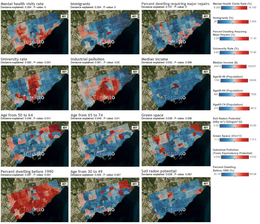
Figure 2: Overview of significant factors used in the analysis of LCPMR. The spatial distributions determined from open data are shown. All of the factors shown are significantly correlated with LCMPR, as determined by GAM analyses. For each factor, the P-value and estimated degrees of freedom (edf) of the significance of the model smooth terms are shown. Factors are ranked by edf. Mental health visits and immigrants are the most significant factors, with deviance-explained values greater than 0.1. The spatial map was created using OpenStreetMap online platform (http://http://www.openstreetmap.org/) ($\copyright$ OpenStreetMap contributors) under the license of CC BY-SA (http://www.openstreetmap.org/copyright). More details of the licence can be found at http://creativecommons.org/licenses/by-sa/2.0/. Line graphs were drawn using Tableau Software for Desktop version 9.2.15 (https://www.tableau.com/zh-cn/support/releases/9.2.15).

Table 1: Factors considered in the analyses of LCPMR in Toronto. * indicates that spatial variations in the data were sufficient for further analysis. All denotes that the variable was included in the best fitting model of all of the neighborhoods. B and C denote that the variable was included in the best fitting model of the neighborhoods in classes B and C, respectively.

Group	Factor	Source(s)	Description	Variation sufficient	Included in best models
Disease	LCPMR	TorontoLCPMR2007	Lung cancer premature mortality rate of premature deaths per 100,000 persons, in the period from 2003 to 2007	*	C,All
Built environment	Industrial pollution	TorontoChem2012 ; NPRI1995	Potential risk of industrial pollutants released by industrial facilities in either 1995 or 2012	*	C,All
Built environment	Dwellings requiring major repairs	TorontoN2011	Percentage of dwellings in need of major repairs in 2011	*	C
Built environment	Green space	Urban2013	Average amount of green space (including parks and public areas) per km2 in a 1-km diameter circular region surrounding each residential block within a neighborhood in 2013.	*	C,All
Built environment	Dwellings constructed before 1990	TorontoN2011	Percentage of dwellings built before 1990	*	B,C
Natural environment	Soil radon potential	chen2008variation	Soil radon potential index to measure risk from soil radon in 2008	*

Table 2: Table 1 continued. Factors considered in the analyses of LCPMR in Toronto. * indicates that spatial variations in the data were sufficient for further analysis. All denotes that the variable was included in the best fitting model of all of the neighborhoods. B and C denote that the variable was included in the best fitting model of the neighborhoods in classes B and C, respectively.

Group	Factor	Source(s)	Description	Variation sufficient	Included in best models
Non-environmental	Mental health visits	AHD2012	Percentage of persons attending mental health visits in 2007. Both sexes, age-adjusted: 20–64.	*	C,All
Non-environmental	Immigrants	ASD2006	Percentage of immigrants present in 2006	*	C,All
Non-environmental	Age from 65 to 74	TorontoCP2006	Population of persons 65–74 years old in 2006	*
Non-environmental	Age from 50 to 64	TorontoCP2006	Population of persons 50–64 years old in 2006	*
Non-environmental	Age from 30 to 49	TorontoCP2006	Population of persons 30–49 years old in 2006	*
Non-environmental	University attendance rate	ASD2006	Percentage of population with a University degree in 2006	*
Non-environmental	Median income in 2006	ASD2006	Median of the weighted total net income of households in 2005, excluding institutional populations	*
Non-environmental	Fruit consumption	IS2012	Percentage of people whose daily vegetable and fruit consumption exceeded five servings in 2012
Non-environmental	Smoking rate	Smoking2007	Percentage of people smoking regularly in 2007
Non-environmental	Physical activity rate	PA2010	Percentage of people having moderately active or higher levels of physical activity during their leisure and commuting time in 2010

METHODS

Figure 3: Overview of the open-data analysis process. (I) Input. Data regarding the target factors were collected and preliminarily processed from available open data sources from three fields (disease, environmental, and non-environmental factors). (II) Methodology. The neighborhoods of the city were classified into different classes based on lung-cancer-related factors. The PCA method was used for dimensional reduction, thereby improving the results obtained from the model-based clustering method. Lastly, GAM was used to study the nonlinear relations between factors and LCPMR. (III) Application. The analysis results for all or specific neighborhoods were summarized.

To address the technical challenges of analyzing the effects of diverse factors on LCPMR, we used the following analysis framework. As depicted in Fig. 3, in the first step, Input, data related to all of the target factors were obtained from available open data sources from three domains (environmental, non-environmental factors, and disease). In the second step, Method, the neighborhoods of the city were classified based on lung-cancer-related factors. The PCA method was used for dimensional reduction, thereby improving the clustering results obtained from the model-based clustering method, in which data’s distributions were modeled by Gaussian distributions. Finally, the generalize additive model (GAM) hastie1990generalized ; wood2006generalized was used to determine the nonlinear relations between factors and LCPMR in all or specific neighborhoods. In the third step, Application, the analysis results of all or specific neighborhoods were summarized.

Industrial data preprocessed using a wind model

In the Toronto case study, it was necessary to preprocess the industrial data using a wind model. Current industrial data indicate the health risks of air pollutants released by factories. However, the spatial range of air pollutants is affected by the wind. Therefore, it is necessary to map the risks of industrial air pollutants onto neighboring spatial locations. We considered two factors in the spreading of pollutants: (1) the potential risk of the pollutants released and (2) the spatial range of the air pollutants. Specifically, a Gaussian model was used to estimate air pollutant dispersion Outline2016 . The pollutant distribution was assumed to follow a Gaussian probability distribution ADMS2016 . The spatial range of pollutants was influenced by wind direction. The potential risk at location $B$ from factory $A$, $R_{F_{A}\rightarrow L_{B}}$, could be modelled as follows:

$$R_{F_{A}\rightarrow L_{B}}\sim log\{R_{TEP}^{A}*P_{Density}^{A\rightarrow B}*P_{Wind}^{A\rightarrow B}\}$$ (1)

where $TEP$ refers to the Toxic Equivalency Potential (TEP) as the potential risks of the pollutants to cause harm TorontoChem2012 . The total $TEP$ from various pollutants released by factory $A$, $R_{TEP}^{A}$, was defined as follows:

$$R_{TEP}^{A}=\sum_{i}V_{TEP_{i}}^{A}$$ (2)

where $V_{TEP_{i}}^{A}$ is the potential risk of the $i$-th pollutant released by factory $A$. The density of pollutants $P_{Density}^{A\rightarrow B}$ released by factory $A$ to location $B$ was assumed to follow a Gaussian probability distribution:

$$P_{Density}^{A\rightarrow B}=Gaussian(\mu,\sigma)$$ (3)

where $\mu$ is the range expectation of highest density, usually within the closest 5 km argo2010chronic . The variance $\sigma$ was set as 1, as the integer which produced the best correlation between the spatial distribution of air pollutants and LCPMR.

Classification methods

To analyze the LCPMR in specific neighborhoods, we classified the neighborhoods based on the target factors to determine their heterogeneity. The classification process consisted of two steps: (1) Dimensional reduction was conducted using PCA on the feature vector, and represented by the first two principals. The percentages of the total variance explained by the two principals were as high as around 98%. (2) Using the two principals of the feature vector, the model-based classification method was used for classification of neighborhoods in Toronto by inferring class categories through the estimation of Bayesian Information Criterion (BIC) (a statistical measure to compare models of different parameter sets).

Nonlinear relation analysis method

To evaluate how various factors were correlated with LCPMR, GAM hastie1990generalized ; wood2006generalized was used to model their nonlinear relations in all and specific neighborhoods. Specifically, $Lc_{i}$, the LCPMR in the $i$-th location was related with specific factors through a link function $g$ as follows:

$$g(Lc_{i})=\sum_{k=1}^{K}f_{k}(x_{k}^{i})$$ (4)

where $x_{k}^{i}$ represents the $k$-th feature of the $i$-th location, and the function $f_{k}$ is a smooth function.

Factor analysis

We analyzed the synthetic nonlinear relations of various factors with LCPMR in Toronto and in specific neighborhoods. However, similar factors may exhibit strong linear relations with each other. Therefore, to reduce interference, we chose to use one of the three significant linearly correlated age factors (percentages of the population aged from 30 to 49, 50 to 64, or 65 to 74), in all of the analyses, and one of the two dwelling-related factors (either percentage of dwellings constructed before 1990 or percentage of dwellings needing major repairs) in the analysis of all of the neighborhoods. Factors with P-values larger than 10% in the synthetic analysis were discarded. The final set of factors consisted of the group with the highest explanation capacity.

RESULTS

In this section, we describe the results of the analyses of all of the neighborhoods and specific classes of neighborhoods.

Factor analysis of all neighborhoods

We first analyzed all of the neighborhoods in Toronto to determine the general relations between various factors and LCPMR using GAM.

The nonlinear analysis results are shown in Fig. 4. The group that best explains the observed LCMPR in Toronto comprise four factors. Two of these factors (industrial pollution and mental health visits) correlate positively with LCPMR. Conversely, the other two factors (immigrants and green spaces) are negatively correlated. Initially, the nonlinear influence of industrial pollution is stable, then increases after reaching a threshold value of around 4. This suggests it is necessary to maintain industrial pollution levels below this threshold. Analysis of green space indicated that its influence on LCPMR increased significantly after exceeding a threshold of around 50.

Figure 4: Overview of nonlinear relations between various factors and LCMPR in all of the neighborhoods. The mean values of the model smooth term are plotted with solid lines, and the confidence intervals are plotted with dashed lines. In addition, the P-value and edf of the significance of the model smooth terms are shown on the x-axes. The overall deviance explained is 0.481.

These results suggest that general trends in the LCPMR can be explained by the following four factors: mental health, immigration, industrial pollution, and green space.

Factor analysis of specific neighborhoods

The deviance explained by the overall analysis was significant but not fine-grained, as the heterogeneity of the neighborhoods was not directly addressed. To further investigate this heterogeneity, the neighborhoods were grouped into three classes identified using an automatic classification method (detailed in the Methods section). As shown in Fig. 1, neighborhoods in Toronto are characterized by different levels of LCPMR. Therefore, we classified these neighborhoods using a model-based classification method to identify different classes of neighborhoods automatically. The classification results are shown in Fig. 5. Three classes were identified with the best BIC. Class A was characterized by low levels of LCPMR; the other two classes (B and C) exhibited high levels of LCPMR, but with different levels of demographic factors. For example, the median income over neighborhoods in class B was $74,495 on average, much higher than that in class C ($44,582). Since class B contained only a small number of neighborhoods, we focused on the single-factor analysis to find its factor with the highest explanatory ability observed. As depicted in Fig. 6, the factor of percentage of dwellings constructed before 1990 was found to be positively correlated with LCPMR, which gave the deviance-explained value as high as 66%. In addition, we chose class C for multi-factor analysis. The analytical results for class C are shown in Fig. 7. The four most significant factors determined in the overall analysis were also significant in class C. Also, two dwelling-based factors were present in the group that best explained the observed LCPMR. Specifically, the percentage of dwellings needing major repairs were positively correlated with LCPMR. The significance of the percentage of dwellings constructed before 1990 initially increased with the percentage, then decreased after reaching a threshold value.

Figure 5: Overview of classification results. The three classes were identified using an classification method to find the best Bayesian Information Criterion (BIC) (a statistical measure to compare models of different parameter sets). There were 61 neighborhoods in class A, 11 in class B and 58 in class C . The spatial map was created using OpenStreetMap online platform (http://http://www.openstreetmap.org/) ($\copyright$ OpenStreetMap contributors) under the license of CC BY-SA (http://www.openstreetmap.org/copyright). More details of the licence can be found at http://creativecommons.org/licenses/by-sa/2.0/. Line graphs were drawn using Tableau Software for Desktop version 9.2.15 (https://www.tableau.com/zh-cn/support/releases/9.2.15). The layouts were modified with Keynote version 6.6.2 (http://www.apple.com/keynote/).

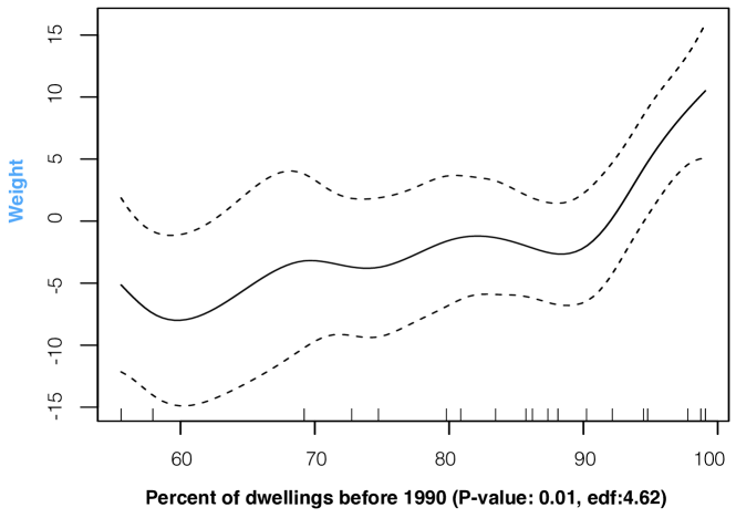
Figure 6: Overview of nonlinear relation between the most significant factor and LCMPR in class B. The mean values of the model smooth terms are plotted with solid lines, and the confidence intervals are plotted with dashed lines. The P-value and edf of the significance of the model smooth terms are shown on the x-axes. The total deviance explained is 0.663.

These findings suggest that the heterogeneity of neighborhoods should not be neglected. The significance of different factors may vary between neighborhoods, which may not be evident in general analysis. Moreover, the deviance is explained better in analyses of specific neighborhoods than in general analyses. In our Toronto case study, the deviance-explained values increased from 48.1% to 80% when the heterogeneity was considered in the multi-factor analysis.

DISCUSSION

We investigated how various factors, analyzed using open data, were connected with disease risks in different neighborhoods of a city. Using Toronto as a case study, we investigated the effects of various factors on Lung Cancer Premature Mortality Rate (LCPMR), and their nonlinear relations were analyzed across the whole city and in specific neighborhoods.

Green space has been shown to promote physical activity and mental health humpel2002environmental ; cohen2015access . Hence, the presence of green space may improve individuals’ health and reduce the LCPMR. Industrial pollution released by factories shows a significant correlation with LCPMR, which may be attributed to the resultant air pollution argo2010chronic . For example, in Canada, people residing in areas exposed to airborne pollutants from industrial releases in 1967-1970 have a higher risk of cancers.

Of the 11 significant lung-cancer-relevant factors identified in the present study, two factors, immigrants and mental health visits, were the most significant factors in determining the LCPMR.

Mental health may be correlated with the LCPMR pirl2012depression , which may result from the influence of depression on people’s health behavior and their use of health care shimizu2012clinical . The lower LCPMR in areas with higher immigrant populations may be attributed to our studied period, which cannot reflect the long-term trend of immigrants’ lung cancer fully. People needed up to 20 years to develop lung cancer de2014spatial . While the immigrants that were studied in this work only settled in Toronto for more than one year in 2006, as compared with the monitored LCPMR period from 2003 to 2007.

Due to the heterogeneity among different neighborhoods, the general relations between factors and LCPMR may not well explain the LCPMR in specific neighborhoods. Thus, it is valuable to determine relations within specific neighborhoods. For example, in class C, the group of factors that best explained the LCPMR contained more factors (six, rather than four) and the deviance-explained value of the best group increased from 48.1% to 80%, compared with the general analysis.

The two additional factors in the class C analysis were both dwelling related, perhaps due to the increased exposure to radon and asbestos in these neighborhoods’ dwellings Asbestos2016 ; lubin1995lung . For instance, dwellings that require major repairs are more likely to have higher concentrations of radon due to inadequate ventilation RadonBuy2016 . Furthermore, dwellings constructed in Toronto before 1990 may contain asbestos in insulation fabricated from vermiculite AsbestosFAQs2016 .

As indicated by comparing the overall analysis and those of specific neighborhoods, geographic heterogeneity should be considered in further research and in public health policy.

The results obtained indicate the correlational relations between various factors and LCPMR. However, they do not indicate the corresponding causal relations. Hence, causal relations should be examined in future studies. Additionally, when calculating the influence of the wind on industrial pollution, the parameters in the wind model were assumed to be homogeneous for all of the industrial facilities across different neighborhoods. Although this limitation may result in some degree of inaccuracy, the measurements reflect the general disparities between Toronto neighborhoods, and therefore the correlations are useful and significant.

The present study provides a flexible framework to investigate the influence of various factors on diseases in cities and in particular neighborhoods thereof. Although the disease and methods used may be particular to the Toronto case study, the questions raised in this study are valuable for similar research in public health using open data. Moreover, this research may be useful to governments in developing future public health policies, and to balance housing, industrial, and health priorities.

CONCLUSION

Based on diverse factors derived from rich open data, the present study aimed to determine their relations to Lung Cancer Premature Mortality Rate (LCPMR) in the heterogeneous neighborhoods of Toronto. To achieve these aims, a flexible framework was developed to recognize potential factors nonlinearly correlated with disease and to determine a set of factors that best explained the observed disease LCPMRs. In addition, clustering of neighborhoods was used to determine heterogeneity.

Taking Toronto as a case study, the convergence of the main factors was used to explain the observed LCPMRs in heterogeneous neighborhoods. Specifically, four significant factors (green space, industrial pollution, immigrants, and mental health visits) were identified in the relational analysis of all of the neighborhoods. To determine the heterogeneity of Toronto’s neighborhoods, we clustered the neighborhoods into three different classes, and conducted an in-depth analysis of the class with the highest LCMPR. Two additional dwelling-related factors were incorporated, which increased the deviance explained from 48.1% to 80%.

The factors influencing diseases in cities become increasingly sophisticated with the development of new physical and social environments. It is possible that some emerging factors that contribute to diseases, such as lung cancer, have not yet been identified. Alternatively, some factors traditionally thought to be unrelated to disease may increase in significance as a result of changes in complex environmental conditions. Based on advances in open data, interdisciplinary collaborations in the analyses of various factors may determine their influences on diseases in heterogeneous regions. The results of this research may guide governments in developing public health policies.

Figure 7: Overview of nonlinear relations between various factors and LCMPR in class C. The mean values of the model smooth terms are plotted with solid lines, and the confidence intervals are plotted with dashed lines. The P-value and edf of the significance of the model smooth terms are shown on the x-axes. The total deviance explained is 0.807.

References

- (1) Diez Roux Ana Victoria. Investigating neighborhood and area effects on health. Am J Public Health. 2001;91(11):1783–1789.
- (2) Macintyre Sally, Ellaway Anne, Cummins Steven. Place effects on health: How can we conceptualise, operationalise and measure them? Soc Sci Med. 2002;55(1):125–139.
- (3) Piccolo Rebecca, Duncan Dustin, Pearce Neil, McKinlay John. The role of neighborhood characteristics in racial/ethnic disparities in type 2 diabetes: Results from the Boston Area Community Health (BACH) survey. Soc Sci Med. 2015;130:79–90.
- (4) Grineski Sara. Incorporating health outcomes into environmental justice research: The case of children’s asthma and air pollution in Phoenix, Arizona. Environ Hazards. 2007;7(4):360–371.
- (5) Corburn Jason, Osleeb Jeffrey, Porter Michael. Urban asthma and the neighbourhood environment in New York City. Health Place. 2006;12(2):167–179.
- (6) Villeneuve Paul, Jerrett Michael, Su Jason, et al. A cohort study of intra-urban variations in volatile organic compounds and mortality, Toronto, Canada. Environ Pollut. 2013;183:30–39.
- (7) Ireton Julie. Full Asbestos Ban, Changed Codes and Regulations Expected by 2018. 2016. http://www.cbc.ca/news/canada/ottawa/asbestos-ban-announcement-1.3895843. Accessed Dec 16, 2016.
- (8) The Mayor’s Office of Data Analytics, The Department of Information Technology, Telecommunications , NYC Digital. NYC Open Data. http://www.nyc.gov/html/data/about.html. Accessed Nov 22, 2016.
- (9) Toronto Public Health. Toronto Open Data. 2012. http://www1.toronto.ca/wps/portal/contentonly?vgnextoid=9e56e03bb8d1e310VgnVCM10000071d60f89RCRD. Accessed Nov 23, 2016.
- (10) Canada Environment. 1994 National Pollutant Release Inventory (NPRI). 1995. http://www.publications.gc.ca/site/eng/9.645899/publication.html. Accessed Nov 23, 2016.
- (11) Howlader Nadia, Noone Anne-Michelle, Krapcho Martin, et al. SEER cancer statistics review, 1975–2008. Bethesda, MD: National Cancer Institute. 2011. https://seer.cancer.gov/archive/csr/1975_2008/. Accessed Nov 22, 2016.
- (12) Stewart Bernard, Wild Christopher. World Cancer Report 2014. http://www.thehealthwell.info/node/725845. Accessed Dec 3, 2016.
- (13) Jemal Ahmedin, Bray Freddie, Center Melissa M, Ferlay Jacques, Ward Elizabeth, Forman David. Global cancer statistics. CA Cancer J Clin. 2011;61(2):69–90.
- (14) Ferlay Jacques, Shin Hai-Rim, Bray Freddie, Forman David, Mathers Colin, Parkin Donald Maxwell. Estimates of worldwide burden of cancer in 2008: GLOBOCAN 2008. Int J Cancer. 2010;127(12):2893–2917.
- (15) Hunt Bijou, Balachandran Banujan. Black: White disparities in lung cancer mortality in the 50 largest cities in the United States. Cancer Epidemiol. 2015;39(6):908–916.
- (16) World Health Organization. Cancer. 2017. http://www.who.int/mediacentre/factsheets/fs297/en/. Accessed Apr 11, 2017.
- (17) Toronto Public Health. The Unequal City: Income and Health Inequities in Toronto. Lung Cancer Incidence, 2008. 2008. http://www.torontohealthprofiles.ca/a_documents/EC_allCateg_charts/EC_charts_AHD/26_ECharts_AHD_LungCancerIncidence.pdf. Accessed Feb 08, 2015.
- (18) Toronto Public Health. The Unequal City 2015: Income and Health Inequities in Toronto. 2015. http://www.toronto.ca/legdocs/mmis/2015/hl/bgrd/backgroundfile-79096.pdf. Accessed Feb 08, 2015.
- (19) Toronto Public Health. Toronto Community Health Profiles, All Socio-demographic (Census). 2006. http://www.torontohealthprofiles.ca/a_dataTables.php?varTab=HPDtbl. Accessed Nov 23, 2016.
- (20) Hystad Perry, Brauer Michael, Demers Paul A, et al. Geographic variation in radon and associated lung cancer risk in Canada. Can J Public Health. 2014;105(1):4–10.
- (21) Crouse Dan L, Peters Paul A, Villeneuve Paul J, et al. Within-and between-city contrasts in nitrogen dioxide and mortality in 10 Canadian cities; a subset of the Canadian Census Health and Environment Cohort (CanCHEC). J Expo Sci Environ Epidemiol. 2015;25(5):482–489.
- (22) Jackson Richard J, Dannenberg Andrew L, Frumkin Howard. Health and the built environment: 10 years after. Am J Public Health. 2013;103(9):1542–1544.
- (23) Berglund Anders, Lambe Mats, Lüchtenborg Margreet, et al. Social differences in lung cancer management and survival in South East England: A cohort study. BMJ Open. 2012;2(3):e001048.
- (24) Casper Michele. A definition of “social environment”. Am J Public Health. 2001;91:465.
- (25) Domínguez-Berjón María Felícitas, Gandarillas Ana, Soto María José. Lung cancer and urbanization level in a region of Southern Europe: Influence of socio-economic and environmental factors. J Public Health. 2016;38(2):229–236.
- (26) Qi Vikky, Phillips Susan P, Hopman Wilma M. Determinants of a healthy lifestyle and use of preventive screening in Canada. BMC Public Health. 2006;6(1):1.
- (27) Jack Ruth, Davies Elizabeth, Møller Henrik. Lung cancer incidence and survival in different ethnic groups in South East England. Br J Cancer. 2011;105(7):1049–1053.
- (28) Brenner Darren, Yannitsos Demetra, Farris Megan, Johansson Mattias, Friedenreich Christine. Leisure-time physical activity and lung cancer risk: A systematic review and meta-analysis. Lung Cancer. 2016;95:17–27.
- (29) Emaus Aina, Thune Inger. Physical activity and lung cancer prevention. Recent Results Cancer Res. 2010;186:101–133.
- (30) Mao Yang, Pan Saiyi, Wen Shi Wu, Johnson Kenneth C, Group Canadian Cancer Registries Epidemiology Research. Physical activity and the risk of lung cancer in Canada. Am J Epidemiol. 2003;158(6):564–575.
- (31) Tomczak Anna, Miller Anthony, Weichenthal Scott, et al. Long-term exposure to fine particulate matter air pollution and the risk of lung cancer among participants of the Canadian National Breast Screening Study. Int J Cancer. 2016;139(9):1958–1966.
- (32) Hong Waun Ki, Tsao Anne. Lung Carcinoma: Tumors of the Lungs. Merck Manual Professional Edition. 2007. http://www.merckmanuals.com/professional/pulmonary-disorders/tumors-of-the-lungs/lung-carcinoma. Accessed Dec 3, 2016.
- (33) Smith Michael. Race, Ethnicity, Social Class: Are Most Urban Neighborhoods Homogeneous or Heterogeneous? 2011. http://wideurbanworld.blogspot.com/2011/08/race-ethnicity-social-class-are-most.html. Accessed Dec 3, 2016.
- (34) York Abigail, Smith Michael, Stanley Benjamin, et al. Ethnic and class clustering through the ages: A transdisciplinary approach to urban neighbourhood social patterns. Urban Stud. 2011;48(11):2399–2415.
- (35) Partnership Toronto Community Health Profiles. Toronto Community Health Profiles. 2012. http://www.torontohealthprofiles.ca/. Accessed Feb 08, 2015.
- (36) Toronto Public Health. Toronto Health Surveillance Indicators. 2013. http://www1.toronto.ca/wps/portal/contentonly?vgnextoid=745d5ce6dfb31410VgnVCM10000071d60f89RCRD&vgnextchannel=9553ebfc2bb31410VgnVCM10000071d60f89RCRD. Accessed Nov 22, 2016.
- (37) Canada Statistics. 2006 Census of Population. 2006. https://www12.statcan.gc.ca/census-recensement/2006/index-eng.cfm. Accessed Nov 23, 2016.
- (38) Canada Statistics. National Household Survey. 2011. https://www12.statcan.gc.ca/nhs-enm/2011/dp-pd/prof/index.cfm?Lang=E. Accessed Nov 23, 2016.
- (39) Toronto Public Health. Toronto ChemTRAC. 2012. http://www1.toronto.ca/wps/portal/contentonly?vgnextoid=63dfad7efc232510VgnVCM10000071d60f89RCRD. Accessed Nov 23, 2016.
- (40) Ruiz Jazmin Del Carmen, Quackenboss James, Tulve Nicolle. Contributions of a child’s built, natural, and social environments to their general cognitive ability: A systematic scoping review. PLoS One. 2016;11(2):e0147741.
- (41) Agency U.S. Environmental Protection. Using a Total Environment Framework (Built, Natural, Social Environments) to Assess Life-long Health Effects of Chemical Exposures. 2016. https://www.epa.gov/research-grants/using-total-environment-framework-built-natural-social-environments-assess-life-long. Accessed Dec 3, 2016.
- (42) National Cancer Institute . Asbestos Exposure and Cancer Risk. 2009. https://www.cancer.gov/about-cancer/causes-prevention/risk/substances/asbestos/asbestos-fact-sheet. Accessed Nov 22, 2016.
- (43) Lubin Jay, Boice John, Edling Christer, et al. Lung cancer in radon-exposed miners and estimation of risk from indoor exposure. J Natl Cancer Inst. 1995;87(11):817–827.
- (44) Yang Aileen, Wang Meng, Eeftens Marloes, et al. Spatial variation and land use regression modeling of the oxidative potential of fine particles. Environ Health Perspect. 2015;123(11):1187.
- (45) Mitchell Richard, Popham Frank. Effect of exposure to natural environment on health inequalities: An observational population study. Lancet. 2008;372(9650):1655–1660.
- (46) Pirl William, Greer Joseph, Traeger Lara, et al. Depression and survival in metastatic non–small-cell lung cancer: Effects of early palliative care. J Clin Oncol. 2012;30(12):1310–1315.
- (47) Brown Patrick, Jiang Hedy, Ezzat Shereen, Sawka Anna M. A detailed spatial analysis on contrasting cancer incidence patterns in thyroid and lung cancer in Toronto women. BMC Public Health. 2016;16(1):950.
- (48) Argo James. Chronic diseases and early exposure to airborne mixtures: Part III. Potential origin of pre-menopausal breast cancers. J Expo Sci Environ Epidemiol. 2010;20(2):147–159.
- (49) López-Cima María Felicitas, García-Pérez José, Pérez-Gómez Beatriz, et al. Lung cancer risk associated with residential proximity to industrial installations: A spatial analysis. Int J Environ Sci Technol. 2013;10(5):891–902.
- (50) Syme Leonard, Ritterman Miranda. The importance of community development for health and well-being. Commun Dev Invest Rev. 2009;5(3):1–13.
- (51) Toronto Public Health. Toronto’s Health Status Indicator Series. Lung Cancer, 2013. 2010. http://www1.toronto.ca/wps/portal/contentonly?vgnextoid=d69e6032bcaa6410VgnVCM10000071d60f89RCRD. Accessed Feb 08, 2015.
- (52) Hastie Trevor, Tibshirani Robert. Generalized Additive Models. CRC Press; 1990.
- (53) Wood Simon. Generalized Additive Models: An Introduction with R. CRC press; 2006.
- (54) Brenner Naama, Bialek William, Van Steveninck Rob de Ruyter. Adaptive rescaling maximizes information transmission. Neuron. 2000;26(3):695–702.
- (55) Bouveyron Charles, Brunet-Saumard Camille. Model-based clustering of high-dimensional data: A review. Comput Stat Data Anal. 2014;71:52–78.
- (56) Bruin Elza C, McGranahan Nicholas, Mitter Richard, et al. Spatial and temporal diversity in genomic instability processes defines lung cancer evolution. Science. 2014;346(6206):251–256.
- (57) Toronto Public Health. Toronto Community Health Profiles, Leading Causes of Premature Mortality. 2007. http://www.torontohealthprofiles.ca/a_dataTables.php?varTab=HPDtbl#. Accessed Nov 22, 2016.
- (58) Partnership Toronto Community Health Profiles. Urban HEART @Toronto Matrix Data. 2013. http://www.torontohealthprofiles.ca/urbanheartattoronto.php. Accessed Mar 26, 2017.
- (59) Toronto Public Health. Toronto Community Health Profiles, Adult Health and Disease. 2012. http://www.torontohealthprofiles.ca/a_dataTables.php?varTab=HPDtbl. Accessed Nov 23, 2016.
- (60) Toronto Public Health. Toronto’s Health Status Indicator Series, 2011-2012. 2012. http://www1.toronto.ca/wps/portal/contentonly?vgnextoid=d69e6032bcaa6410VgnVCM10000071d60f89RCRD. Accessed Nov 23, 2016.
- (61) Toronto Public Health. Toronto’s Health Status Indicator Series. Smoking, 2007-2008. 2008. http://www1.toronto.ca/wps/portal/contentonly?vgnextoid=a3f5515015a89510VgnVCM10000071d60f89RCRD. Accessed Feb 08, 2015.
- (62) Toronto Public Health. Toronto’s Health Status Indicator Series. Physical Activity, 2009-2010. 2010. http://www1.toronto.ca/wps/portal/contentonly?vgnextoid=a3f5515015a89510VgnVCM10000071d60f89RCRD. Accessed Feb 08, 2015.
- (63) Chen Jing, Ly Jim, Bergman Lauren, Wierdsma J, Klassen RA. Variation of soil radon concentrations in southern Ontario. Radiat Prot Dosimetry. 2008;131(3):385–389.
- (64) Wikipedia Contributors. Outline of Air Pollution Dispersion — Wikipedia, The Free Encyclopedia. https://en.wikipedia.org/wiki/Outline_of_air_pollution_dispersion. Accessed Nov 23, 2016.
- (65) Cambridge Environmental Research Consultants. ADMS 5. http://www.cerc.co.uk/environmental-software/ADMS-model/options.html. Accessed Nov 23, 2016.
- (66) Humpel Nancy, Owen Neville, Leslie Eva. Environmental factors associated with adults’ participation in physical activity: A review. Am J Prev Med. 2002;22(3):188–199.
- (67) Cohen-Cline Hannah, Turkheimer Eric, Duncan Glen E. Access to green space, physical activity and mental health: A twin study. J Epidemiol Community Health. 2015;69(6):523–529.
- (68) Shimizu Ken, Nakaya Naoki, Saito-Nakaya Kumi, et al. Clinical biopsychosocial risk factors for depression in lung cancer patients: A comprehensive analysis using data from the Lung Cancer Database Project. Ann Oncol. 2012;23(8):1973–1979.
- (69) United States Environmental Protection Agency. Home Buyer’s and Seller’s Guide to Radon. 2013. https://www.epa.gov/radon/home-buyers-and-sellers-guide-radon. Accessed Nov 22, 2016.
- (70) Canadian Environmental Law Association. Asbestos: FAQs. 2012. http://www.cela.ca/faq/findlegalhelp.ca?page=1&tid=All. Accessed Nov 22, 2016.