New methods to generate massive synthetic networks

Abstract.

One of the biggest needs in network science research is access to large realistic datasets. As data analytics methods permeate a range of diverse disciplines—e.g., computational epidemiology, sustainability, social media analytics, biology, and transportation— network datasets that can exhibit characteristics encountered in each of these disciplines becomes paramount. The key technical issue is to be able to generate synthetic topologies with pre-specified, arbitrary, degree distributions. Existing methods are limited in their ability to faithfully reproduce macro-level characteristics of networks while at the same time respecting particular degree distributions. We present a suite of three algorithms that exploit the principle of residual degree attenuation to generate synthetic topologies that adhere to macro-level real-world characteristics. By evaluating these algorithms w.r.t. several real-world datasets we demonstrate their ability to faithfully reproduce network characteristics such as node degree, clustering coefficient, hop length, and k-core structure distributions.

1. Introduction

Network science has made inroads into a variety of domains  (Kleinberg et al., 1999),

(Kumar et al., 2000),  (White et al., 1986),  (Camacho et al., 2002),  (Guelzim et al., 2002),  (Jeong et al., 2003),  (Ebel et al., 2002) including epidemiology, sustainability, health informatics, and transportation. As the scope of such applications continues to broaden, data analytics research needs a constant supply of realistic datasets that mimic characteristics encountered in these domains.

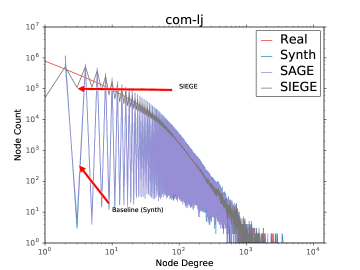
Figure 1. This plot demonstrates how our proposed model SIEGE captures real topology characteristics better than the baseline Synth when used to mimic the com-LiveJournal dataset (3.99 million nodes and over 34 million edges).

A key need is to have synthetic network representations that reproduce macro-level behavior found in real networks. Examples of phenomena we wish to study using synthetic networks include: robustness:- against targeted and random removal of nodes and edges, homophily:- whether nodes that share similar characteristics tend to have more edges between them, search:- to understand the impact on search strategy with respect to network topology, and diffusion processes:- the spread of dynamics over a network. Having realistic synthetic network representations supports privacy concerns and can help realize what-if studies that are not possible to conduct in real life. We abstract the essential problem as one of creating synthetic networks with arbitrary, user-specified, degree distributions.

The primary contributions of this paper are:

• Weakness analysis. We begin by demonstrating that state-of-the-art techniques for generating networks with arbitrary degree distributions are found wanting. In particular, we demonstrate that the well known DEG method (Heath and Parikh, 2011) falls short when evaluated against real characteristics (broadly summarized as triadic closures growing superlinearly in the number of edges in the topology).

• Proposal of new models. We propose a fail safe baseline Synth that is more stable than DEG, and propose two more models SAGE , SIEGE that outperform it, in terms of generating synthetic topologies with adherence to macro level real world characteristics. This can be seen using the annotations in the Figure 1 (shown in log-log scale). SAGE and SIEGE uses the principle of residual degree attenuation (to be described in a later section).

• Extensive experiments and evaluations to validate the effectiveness of our proposed models. We compare our synthetically generated networks against 25 real-world datasets w.r.t. five well accepted characteristics, demonstrating consistent superiority in reproducing these characteristics.

2. Related Work

Related research in this area can be understood from three viewpoints (Nettleton, 2015): synthetic topology generation without data, synthetic topology generation followed by data generation to fit the topology ((Barrett et al., 2009), (Pérez-Rosés and Sebé, 2015)) and finally the notion of like liking like otherwise known as homophily (and it’s counterpart concept diversity) (McPherson et al., 2001). Among these three viewpoints the first has the lions share in terms of past research. Note that we will touch upon the related work from this viewpoint, as our work serves to extend this approach.

2.1. Synthetic topology generation without data

(a) Random Topology

(b) Scale-Free Topology

Figure 2. A random topology model such as the Erdos-Renyi model converges to a Poisson degree distribution while a scale-free topology tends to have fewer nodes with high degrees and more nodes with smaller degrees. On a log-log scale of node count vs node degree the curve would be linear, oblique and heavy tailed.

2.1.1. ER Model:

Solomonoff et al.(Solomonoff and Rapoport, 1951) and Erdos et al.(Erdös and Rényi, 1960) independently presented a model of graph topology generation with n nodes where each pair of nodes can have an edge between them with a probability p. In this method the probability of having a graph with n nodes and l edges is ${L\choose l}p^{l}(1-p)^{L-l}$ , where $L={n\choose 2}$, which is the maximum possible number of edges in a graph. The degree distribution is approximately Poisson. Networks generated by this model do not satisfy properties such as the small-world phenomenon.

2.1.2. Small-world Networks:

Networks generated by the ER model do not exhibit local clustering and triadic closures. The degree distribution converges to a Poisson distribution instead of a power law which most scale-free real world networks tend to exhibit (see Fig. 2). Watts et al.(Watts and Strogatz, 1998) proposed a small-world model, for n nodes, mean degree k and parameter p where $0\leq p\leq 1$, to produce a network with n nodes and nk/2 edges. The limitation of this method is that it generates non-scale free networks. The two step generation process works as follows:

1) Construct a regular ring lattice with n nodes each connected to k of its neighbors with k/2 nodes on each side.

2) Rewire every edge with probability p, such that $(n_{i},n_{j})$ is replaced with $(n_{i},n_{k})$ where k is chosen with uniform probability from all possible values such that there are no self-loops and link-duplication.

The degree distribution of the topology is a Dirac-delta function centered at k for the ring lattice and is Poisson distributed in the limiting case of $p\to 1$. If $p=0$ then the graph is a regular ring lattice with clustering coefficient $C=\frac{3k-3}{4k-2}$ and the diameter $\frac{n}{4k}$ for large n. If $p=1$ then the graph is completely random with diameter $\frac{\log n}{logk}$ and clustering coefficient $C=\frac{2k}{n}$ which is a low value. Between the two extremities of $p=0$ and $p=1$ there exists a region that gives low diameter and high clustering coefficient, the charactristics of a small-world network.

To overcome its inability to generate scale-free networks, Newman et al.(Newman and Watts, 1999) proposed a variant where for each edge in the network with probability $p$ a new edge is added between two randomly chosen nodes. The degree distribution of this network is also non-conforming to real world as it is uniform for the lattice and binomially distributed for the randomly added edges.

2.1.3. Preferential Attachment Model.

This class of algorithm is based on the principle of ”cumulative advantage” as stated by Price (Price, 1976) to describe citation networks: the probability that one comes across a paper while reading the literature is intuitively proportional to the number of papers citing it. Barabasi et al.(Barabási and Albert, 1999) rediscovered the notion by considering an undirected graph and named the phenomenon as ‘preferential attachment.’ In their algorithm the network initially begins with $m_{0}$ connected nodes. New nodes are added to the existing network one at a time. Each new node is connected to m existing nodes in the network where $m\leq m_{0}$ and the probability $P$ that a new node connects to an existing node $v$ is proportional to the degree of $v$, $d[v]$. Thus $P(d[v])=\frac{d[v]}{\sum_{i=1}^{n}d[i]}$. Barabasi et al. (Barabási and Albert, 1999) also showed that this method leads to topologies with degree distribution that follows a power law $p_{k}\propto k^{-\alpha}$ where $\alpha=3$. The clustering coefficient also increases with network size as $C\approx N^{-0.75}$, a behavior that is different from small-world networks where clustering tends to be independent of system size. Adamic et al. (Adamic and Huberman, 2000) provided empirically observed properties of the web link structure to highlight shortcomings of the Barabasi et al. model. Several variants of the PA model exist, a selected list of which is listed here. Holme et al. (Holme and Kim, 2002) proposed a model that at first has a preferential attachment step where a new node v is attached to an existing node w with the probability proportional to the degree of w. This is followed by a triad formation step. where the new node v is connected to randomly chosen neighbor u of the node w that was selected as attachment site in the PA step. If there remains no pair to be connected, i.e., if all neighbors of w are already connected to v, then a PA step is done instead. Guo et al. (Guo et al., 2006), proposed a simple algorithm that generated a scale-free small world network that is similar to Holme et al. (Holme and Kim, 2002) in that it too adds a new node v with m edges at each time step. In the first step, each edge of v is attached to an existing node with a probability proportional to it’s degree. The second step involves attaching the new node v to a randomly chosen neighbor s of w (w being the nodes which has edges between itself and v) with probability given by $p_{s}=\frac{d[s]^{\beta}}{\sum_{i\in r_{w}}d[i]^{\beta}}$ where d[i] is the degree of node i, $r_{w}$ is the set of neighbors of w and $\beta$ is the preferential exponent parameter. This model can generate a non-trivial clustering property. Wang et al. (Wang et al., 2008) introduced a model that at each time step added a new node v with m edges. A node u is selected at random such that the local world of v is u(s) which is the set of all nodes that are at a distance of s or less from u. The node v does a preferential attachment to node $w\in u(s)$. Followed by which v connects itself to the highest degree neighbor of node w with a probability p, which also acts a parameter for tuning clustering coefficient. Schank et al. (Schank and Wagner, 2004) proposed a model where at each time step a new node with m edges is added to previously existing nodes by following a PA step. Then as a second step, for each node $v\in V$, two neighbors u and w are selected at random and are connected. The clustering coefficient can be varied by varying the number of times the second step is repeated.

Guo et al.(Guo and Kraines, 2009) proposed a model that generated directed graphs where in-degree and out-degree follows power law. The algorithm uses the power exponent for in-degree and out-degree to generate the in-degree and out-degree sequence along with number of nodes n and edges m. Following this step, out-stubs and in-stubs are randomly assigned to vertices as per the degree sequence. Finally, links are created between randomly between in-stubs and out-stubs with some probability. The average clustering coefficient ($C_{f}$) of the graph thus obtained tends to be lower than the specified input. In those cases edge switching occurs to increase the $C_{f}$ for some nodes, according to the following set of rules:- A random node $v$ and four distinct nodes $w,x,y,$ and $z$ are chosen, such that,

1. $w$ and $x$ are neighbors of $v$

2. $y$ and $z$ are not neighbors of $v$

3. $(w,x)\notin E$ and $(z,y)\notin E$

4. $(w,y)\in E$ and $(z,x)\in E$

5. $C(v)$ of neighbors shared by $w$ and $y<targetC_{f}$

6. $C(v)$ of neighbors shared by $x$ and $z<targetC_{f}$

On deleting edges $(w,y)$ and $(z,x)$ from $E$, and adding edges $(w,x)$ and $(z,y)$ to E would increase the local $C_{f}$ of the node $v$, which contributes to increasing global $C_{f}$ of the network. Gleeson et al.(Gleeson, 2009) proposed a model that uses the joint probability distribution function $\gamma(k,c)$, which gives the probability that a randomly chosen node in the network will have a degree k and would belong to a c-clique. The network is generated by connecting stubs (viewed as external edges) to these cliques. This method generates graphs with n-adic structures as opposed to just triadic as is prevalent in many methods. However, it is still not realistic as real-world networks need not have nodes that are constrained to be part of a single clique.

2.1.4. Configuration Model

Molloy et al. (Molloy and Reed, 1995) proposed the configuration model, wherein given the degree distribution (d[1], d[2] … d[n]) of n nodes as input it creates a set Q having d[i] distinct copies of each node i and then selects two nodes at random from the set Q and adds an edge between them. This process is repeated until every element is part of some edge. It produces a multigraph from which a simple graph can be obtained by merging the multi-edges and removing the self-loops. Heath et al. (Heath and Parikh, 2011) proposed a model called DEG that takes a degree sequence and a target clustering coefficient and tries to generate a simple random graph with these properties. It is based on the configuration model, i.e., each node $v$ is seen as having a finite number of stubs coming out of it, which is equal to the degree of the node $d[v]$. The next step, in this model, is to calculate the total number of triangles that are required to achieve the given clustering coefficient, and then create those by selecting three stubs, guided by the residual degree distribution, and joining them to create a triangle. Once the estimated number of triangles is created, a pair of stubs are selected, again guided by the residual degree distribution, and joined to create additional edges. This model is limited in generating synthetic networks that conforms to real world network statistics if the total number of triangles required exceeds the total number of edges provided in the graph, which almost invariably is the case with real world networks as they follow power law degree distribution. To overcome this shortcoming, we propose three new DEG-inspired models and measure the statistics they generate with the real world network statistics we choose to replicate.

3. Definitions

Let $G=(V,E)$ be an undirected simple graph with a set of nodes $V$ and a set of edges $E$. The cardinality of $V$, i.e $|V|=n$ and $|E|=m$. The degree $d(v)=|{u\in V:\exists\{u,v\}\in E}|$ of a node $v$ is the count of all nodes that are adjacent to $v$. A complete graph on n nodes is $K_{n}$, and a complete r-partite graph with partition of size $(n_{1},n_{2}...n_{r})$ is $K_{n_{1},...n_{r}}$. A triangle $\Delta=(V_{\Delta},E_{\Delta})$ of a graph $G=(V,E)$ is a three node subgraph with $V_{\Delta}=\{u,v,w\}\subseteq V$ and $E_{\Delta}=\{(u,v),(v,w),(u,w)\}\subseteq E.$ The number of triangles at a node $v$ is given by

(1) $$\Delta(v)=|\{(u,w)\in E|(v,u)\in E\ and\ (v,w)\in E\}|.$$

The number of triples at a node v is the number of length 2 paths in which v is the central node. It can be quantified as

(2) $$\tau(v)={d[v]\choose 2}.$$

The local clustering coefficient $C(v)$ is the ratio of the number of triangles at node v to the number of triples,, i.e,

(3) $$C(v)=\frac{\Delta(v)}{\tau(v)}\ \mbox{if}\d{[}v]\geq 2.$$

The clustering coefficient of the graph $C(G)$ for the graph $G(V,E)$ is defined as the average of $C(v)$ of all nodes $v$ in the graph. That is,

(4) $$C(G)=\frac{1}{|V|}\sum_{v\in V}C(v).$$

The total number of triangles in a graph in terms of $\Delta(v)$ is

(5) $$\Delta(G)=\frac{\sum_{v\in V}\Delta(v)}{3}$$

as each triangle constitutes three nodes.

The number of triples in the graph is

(6) $$\tau(G)=\sum_{v\in V}\tau(v).$$

The global clustering coefficient $C_{g}(G)$ is defined as three times the number of triangles in the graph to the number of triples in the graph, that is

(7) $$C_{g}(G)=\frac{3\Delta(G)}{\tau(G)}$$

If the total number of connected components in the graph is $\lambda$, then a cut edge or edge bridge $(u,v)\in E$ is an edge which if removed from the graph, changes the total number of connected components to $\lambda^{{}^{\prime}}$ where $\lambda^{{}^{\prime}}-\lambda=1$. A path from a node $u$ to $v$ in a graph $G$ is a sequence of edges $\{(x_{0},x_{1}),....,(x_{n-1},x_{n})\}$, where $x_{0}=u$ and $x_{n}=v$. The hop length is the one that has the minimum number of edges among all such possible paths between any two given vertices in the graph. Finally, the connected components that are left after all vertices of degree less than k have been removed are defined as the k-cores of the graph.

3.1. Dynamics on Networks

The above definitions capture structural properties of networks. We are also interested in dynamics exhibited by networks. For the purpose of this paper, we focus on the SIR epidemiological model  (Kermack and McKendrick, 1927) wherein a node can go through three stages during the course of the dynamics:

• Susceptible: Before the node has been infected it is susceptible to infection from any of its neighbors.

• Infectious: Once infected, it is capable of infecting any of its susceptible neighbors

• Recovered: Once the required time period of infection for that node is over it is considered as recovered.

Assuming S is the proportion of population that is susceptible, I is the proportion of the population that is infected and R is the proportion that has recovered, $\beta$ being the transmission rate among the individuals and $\gamma$ being the recovery rate we have,

$$\frac{dS}{dt}=-\beta SI\ \text{,}\ \frac{dI}{dt}=\beta SI-\gamma I\ \text{,}\ \frac{dR}{dt}=\beta I$$

This also assumes there is no birth, death or migration of populations. Thus new nodes are not allowed to be created. Our goal is to evaluate our synthetic networks against SIR dynamics imposed on them versus SIR dynamics on real networks.

4. Models

4.1. Making DEG work in practice

It is noted that an n-clique has exactly $n\choose 3$ triangles and asymptotically $\Delta(G_{n-clique})\in\Theta(n^{3})$. We also know that $|E|\in\Theta(n^{2})$. Thus $\Delta(G_{n-clique})\in\Theta(|E|^{3/2})$ (Schank and Wagner, 2005). A n-clique has by definition maximum number of edges possible in a n node graph. If we fix the total number of nodes and want to accommodate as many edges as possible within the clique we can have a family of Graphs $G_{|E|}$ which are not cliques but $\Delta(G_{|E|})\ \mbox{would still be}\ \Theta(|E|^{3/2}))$. This shows, it is very much possible that networks can have more triangles than the total number of edges and in all those cases DEG fails. We propose an algorithm Synth , that gets around this problem. The change proposed is seen in line 7 where the number of triangles to be created is rationed by the number of edges available. For most real world networks, the number of triangles that needs to be created exceeds the number of edges provided. In those cases Synth will run to completion as opposed to DEG. However, it will have a higher chance of generating a singular connected component (or few but large connnected components) as a representation of the graph for most real networks as all edges are exhausted in an effort to reach the delineated number of triangles. This might not be representative of the actual structure which tends to have multiple connected components. It should be noted that it is not a rigorous necessity for the total number of triadic closures, to be more than the total number of edges in order for DEG to stall. Even if it is reasonably close to the number of edges, the algorithm can still stall given the fact that, on an average it consumes more than one unique edge in order to generate a triadic closure. (The oregon010331 to oregon010428 dataset in Table 1 described later serve well to illustrate the purpose.) The algorithm DEG also re-computes the residual degree distribution after each successful sampling of at-most 3 unique edges. This does not affect the runtime as long as the count of the following two factors are within reasonable bounds:

• $|E_{G_{n}}|<<|E_{G_{n-clique}}|$, as this evidently reduces the number of loop iterations.

• $|V|\approx 10^{3}$ , as this results in fast re-normalization of the residual degree distribution once 3 (at-most) unique edges are sampled.

But as we attempt to generate larger synthetic datasets the aforementioned factors tend not to hold true anymore thus leading to scalability issues. To overcome this issue, we conduct bulk edge sampling by taking a snapshot of the residual degree distribution at iteration points which are tuned by the step size of our choice. This automatically reduces the number of re-normalization computation by a factor of step-size thus also reducing the computation time by a significant amount while sacrificing some accuracy. However, since this bulk sampling will be applied with uniform step-size for any given large dataset across all the algorithms proposed, the relative accuracy among them should not be affected. It should be noted that this does not mean that the three algorithms will have the same absolute error margins, but that the relative error variations should be invariant given a non-zero step size.

4.2. New Models

Algorithm 1 Synth

1:procedure $Synth$(n,d,$C_{g}(G)$,Step)

2:     $V\leftarrow\{1,2...,n\}$

3:     $E\leftarrow\phi$

4:     $M\leftarrow\frac{\sum_{x\in V}d[x]}{2}$

5:     $rd\leftarrow d$

6:     $T\leftarrow\frac{C_{g}(G)\sum_{i=1}^{n}{d[i]\choose 2}}{3}$

7:     while $T>0\ \textit{and}\ M>0$ do

8:         $\textit{smpl}\leftarrow 0$

9:         $\mbox{Compute}\forall p\in V\frac{rd[p]}{\sum_{x\in V}rd[x]}$

10:         while $T>0\ \textit{and}\ M>0\textit{and smpl}<Step$ do

11:              Choose three distinct nodes

12:              $\mbox{u with probability}\frac{rd[u]}{\sum_{x\in V}rd[x]}$

13:              $\mbox{v with probability}\frac{rd[v]}{\sum_{x\in V}rd[x]}$

14:              $\mbox{w with probability}\frac{rd[w]}{\sum_{x\in V}rd[x]}$

15:              $\mbox{Check}\ rd[u],rd[v],\mbox{and}\ rd[w]$

16:              Add edges needed to create a triangle

17:              $\mbox{between the chosen nodes}\ u,v,\mbox{and}\ w$

18:              $\mbox{update}\ rd[u],rd[v],rd[w],\ T,\textit{smpl}\ \mbox{and}\ M\ \mbox{accordingly}$               

19:     while $M>0$ do

20:         $\textit{smpl}\leftarrow 0$

21:         $\mbox{Compute}\forall p\in V\frac{rd[p]}{\sum_{x\in V}rd[x]}$

22:         while $M>0\textit{and smpl}<Step$ do

23:              Choose two distinct nodes

24:              $\mbox{u with probability}\frac{rd[u]}{\sum_{x\in V}rd[x]}$

25:              $\mbox{v with probability}\frac{rd[v]}{\sum_{x\in V}rd[x]}$

26:              $smpl\leftarrow smpl+1$

27:              if $(u,v)\notin E$ then

28:                  $E\leftarrow E\cup\{(u,v)\}$

29:                  $rd[u]\leftarrow rd[u]-1$

30:                  $rd[v]\leftarrow rd[v]-1$

31:                  $M\leftarrow M-1$                             return $(V,E)$

4.2.1. Synthetic Attenuated Generation Engine (SAGE )

We propose another variant, SAGE where the residual degree of $u,v$ is reduced by $1$ if a new edge $\{(u,v)\}$ is added to the graph but the decrement is attenuated after the residual degree hits 1. The edge addition from line 9 onwards, however, allows the node degree to reduce to 0, as that ensures a node that contributes a new edge is not selected again. Note this holds good even in the worst case when there is no triangle in the graph.In such a scenario the maximum possible number of edges $m$ to fill would be $\lfloor\frac{n^{2}}{4}\rfloor$ (Mantel’s Theorem) (Mantel, 1907) which is only possible on a complete bipartite graph $K_{\lfloor\frac{n}{2}\rfloor,\lceil\frac{n}{2}\rceil}$, and can be successfully processed with a uniform degree distribution, which is almost always the outcome after line 8, for all executions of generating synthetic topology imitating real world networks. The rationale for keeping step size has already been covered in the previous section.

Algorithm 2 SAGE

1:procedure $SAGE$(n,d,$C_{g}(G)$,Step)

2:     $V\leftarrow\{1,2...,n\}$

3:     $E\leftarrow\phi$

4:     $M\leftarrow\frac{\sum_{x\in V}d[x]}{2}$

5:     $rd\leftarrow d$

6:     $T\leftarrow\frac{C_{g}(G)\sum_{i=1}^{n}{d[i]\choose 2}}{3}$

7:     Repeat line 7 to 18 from Synth

8:     but $\mbox{update}\ rd[u],rd[v],rd[w],\ \mbox{only if they are}>1$

9:     while $M>0$ do

10:         $\textit{smpl}\leftarrow 0$

11:         $\mbox{Compute}\forall p\in V\frac{rd[p]}{\sum_{x\in V}rd[x]}$

12:         while $M>0\textit{and smpl}<Step$ do

13:              Choose two distinct nodes

14:              $\mbox{u with probability}\frac{rd[u]}{\sum_{x\in V}rd[x]}$

15:              $\mbox{v with probability}\frac{rd[v]}{\sum_{x\in V}rd[x]}$

16:              $smpl\leftarrow smpl+1$

17:              if $(u,v)\notin E$ then

18:                  $E\leftarrow E\cup\{(u,v)\}$

19:                  if $rd[u]\geq 1$ then

20:                       $rd[u]\leftarrow rd[u]-1$                   

21:                  if $rd[v]\geq 1$ then

22:                       $rd[v]\leftarrow rd[v]-1$                   

23:                  $M\leftarrow M-1$                             return $(V,E)$

4.2.2. Synthetic Isthmus based Edge Generator Engine (SIEGE )

Finally, we propose another variant SIEGE that uses the total number of edge bridges (isthmus) in the original network, as well as the target clustering coefficient to create the synthetic network. (Tarjan, 1974) proposed a linear time model to find the isthmus’ in a given graph. We can modify that a little by keeping a counter (captured by the input parameter $EB_{Count}$ (edge bridge count, please refer table 2), which we provide as input to SIEGE) and thus find the cardinality of the set of isthmus’ in the graph. Also this approach does not require a single edge degree distribution to be stored as compared to (Newman, 2009) making it space efficient. In this algorithm, when execution is at line 3, then either of the two cases happen:-

• The total number of triangles required is generated and more edges are available. In this case the residual edge count is replaced by edge bridge count and the execution is purely focused on generating new edges which has a much higher probability of generating stubs as opposed to triangles.

• In the other scenario, when the edge count is exhausted without reaching the goal of the requisite number of triangles, the algorithm then purely generates single edges from an uniform residual degree distribution, and residual degree count is allowed to reach 0, such that unique nodes can be selected at each iteration.

The topologies generated by this on an average comes closest to real world networks as compared to Synth and SAGE . However, this method uses more edges than the original network topology provides.

Algorithm 3 SIEGE

1:procedure $SIEGE$(n,d,$C_{g}(G)$,Step,$EB_{Count}$)

2:     Repeat line 2 to 8 from SAGE

3:     while $EB_{Count}>0$ do

4:         $\textit{smpl}\leftarrow 0$

5:         $\mbox{Compute}\forall p\in V\frac{rd[p]}{\sum_{x\in V}rd[x]}$

6:         while $EB_{Count}>0\textit{and smpl}<Step$ do

7:              Choose two distinct nodes

8:              $\mbox{u with probability}\frac{rd[u]}{\sum_{x\in V}rd[x]}$

9:              $\mbox{v with probability}\frac{rd[v]}{\sum_{x\in V}rd[x]}$

10:              $smpl\leftarrow smpl+1$

11:              if $(u,v)\notin E$ then

12:                  $E\leftarrow E\cup\{(u,v)\}$

13:                  if $rd[u]\geq 1$ then

14:                       $rd[u]\leftarrow rd[u]-1$                   

15:                  if $rd[v]\geq 1$ then

16:                       $rd[v]\leftarrow rd[v]-1$                   

17:                  $EB_{Count}\leftarrow EB_{Count}-1$                             return $(V,E)$

5. Experimental Setup

5.1. Datasets

We downloaded twenty five topology datasets/statistics (detailed in Table 1) from SNAP (the Stanford Network Analysis Project) and used these statistics as input parameters to our three algorithms to generate three synthetic topologies for each. The twenty five topologies are broadly classified into six categories which are listed as follows:

Table 1. It can be seen that the number of triangles are either more or close to the number of edges in the dataset. DEG works primarily if the number of triangles are significantly less than the number of edges. Most real world networks do not adhere to this characteristic.

Topology  Characteristics
Topology	$|V|$	$|E|$	$|\Delta|$	Diam	EDiam	Step
egoFacebook	4039	88234	1612010	8	4.7	1
caGrQc	5242	14496	48260	17	7.6	1
caHepTh	9877	25998	28339	17	7.4	1
oregon010331	10670	22002	17144	9	4.4	1
oregon010407	10729	21999	15834	11	4.5	1
oregon010414	10790	22469	18237	9	4.4	1
oregon010421	10859	22747	19108	10	4.4	1
oregon010428	10886	22493	17645	10	4.4	1
oregon020331	10900	31180	82856	9	4.3	1
oregon020407	10981	30855	78138	11	4.3	1
oregon020414	11019	31761	88905	8	4.2	1
oregon020421	11080	31538	82029	9	4.3	1
oregon020428	11113	31434	78000	9	4.2	1
oregon020505	11157	30943	72182	9	4.3	1
oregon020512	11260	31303	72866	9	4.2	1
oregon020519	11375	32287	83709	9	4.3	1
oregon020526	11461	32730	89541	9	4.3	1
email-Enron	36692	183831	727044	11	4.8	1000
loc-gowalla	196591	950327	2273138	14	5.7	1000
loc-brightkite	58228	214078	494728	16	6	1000
com-amazon	334863	925872	667129	44	15	10000
com-dblp	317080	1049866	2224385	21	8	10000
com-youtube	1134890	2987624	3056386	20	6.5	20000
com-lj	3997962	34681189	177820130	17	6.5	40000
as-skitter	1696415	11095298	28769868	25	6	20000

• Social Network: This domain includes ego-Facebook (McAuley and Leskovec, 2012)which is an undirected topology dataset collected from survey participants using the facebook app. This dataset is completely anonymized by substituting the facebook internal ids with a new value.

• Autonomous Systems Based Network: We use fifteen topologies from this domain, five of which are oregon1$\_$010 {331 to 428} (Leskovec et al., 2005). These undirected topologies are representations of autonomous systems peering information that were inferred from Oregon route views from $31^{st}\ March\ 2001$ to $28^{th}\ April\ 2001$. Nine, (oregon$\_$020 {331 to 526}), are generated by combining Oregon route-views, looking glass data, and routing registry. Finally we have, as-skitter which is an undirected internet topology graph, from traceroutes run daily in 2005. It has around 1.7 million nodes and 11 million edges.

• Collaboration Network: The topology ca-Gr-Qc is an Arxiv GR-QC (General Relativity and Quantum Cosmology) collaboration network and covers scientific collaborations between authors papers submitted to the General Relativity and Quantum Cosmology category. The topology ca-Hep-Th represents the same idea but for the High Energy Physics category.

• Communication Network: The topology email-Enron is an Enron email communication network (Leskovec et al., 2009; Klimt and Yang, 2004). This covers around half million emails and was originally made public by the Federal Energy Regulatory Commission during its investigation. Nodes of the network are email addresses and if an address i sent at least one email to address j, the graph contains an undirected edge from i to j.

• Location based OSN: The topology loc-gowalla is from Gowalla which is a location-based social networking website where users share their locations by checking-in. This data (Cho et al., 2011) was collected using public API from a total of 6,442,890 check-ins of these users over the period of Feb. 2009 - Oct. 2010. We also use another topology loc-brightkite that is similar to the Gowalla based dataset (Cho et al., 2011) which was collected from a total of 4,491,143 checkins of these users over the period of Apr. 2008 - Oct. 2010.

• Networks with ground-truth communities: We use four topologies, namely com-DBLP, com-Youtube, com-Amazon, com-Livejournal (Yang and Leskovec, 2015). The Amazon network was collected by crawling Amazon.com. It is based on product co-purchasing recommendations that is, if a product i is frequently co-purchased with product j then the graph contains an undirected edge from i to j. DBLP is a co-authorship network where two authors are connected if they have published at least one paper together. In the Youtube social network, users form friendship relationships with each other along the lines of Facebook. Finally livejournal is an online blogging community where users can declare friendships. All these community datasets have edges close to or exceeding 1 million thus making them ideal candidates for large scale replication.

5.2. Baseline and Evaluation Metrics

We use the real world topology with our three synthetic topologies and compare them (Figure 4) using five well accepted characteristics which are: clustering coefficient distribution, node degree distribution, hop length distribution, k-core vs core node distribution, and k-core vs core edge distribution. We also measured the resultant global clustering coefficient of the synthetic network topologies and present those results in Table 2. For large datasets, that is, the last 8 rows of Table 1 we use step size varying from 1000 (email-Enron, loc-gowalla, loc-brightkite), 10,000 (com-amazon, dblp), 20,000 (com-youtube) to 40,000 (com-lj). Exact values will not affect the relative accuracy wrt to the baseline which is our measurement goal. For the rest of the dataset Step is 1, so we remove it altogether from the algorithm . Finally we also run the SIR model based epidemiological simulation on these datasets and their synthetic counterparts and show the infection and recovery count of the affected members of the population in Figure 3. The algorithm DEG would not run in most cases as pointed out in the beginning of the algorithm section. We use the least changed algorithm wrt DEG as our baseline, which in this case happens to be Synth and we show how SAGE and SIEGE outperforms it and ipsofacto outperforms DEG as well.

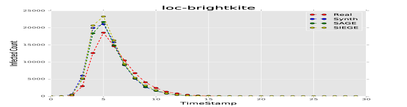
(a)

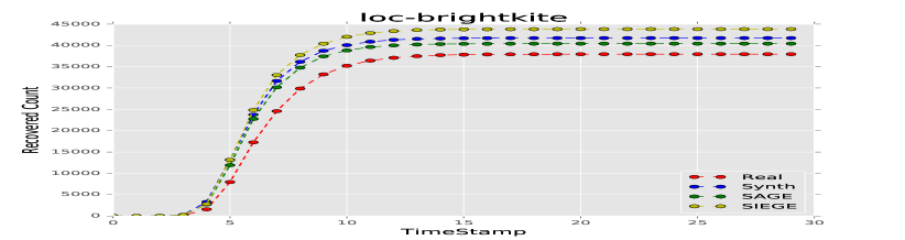
(b)

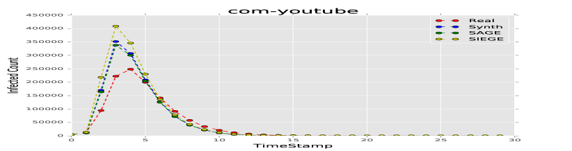
(c)

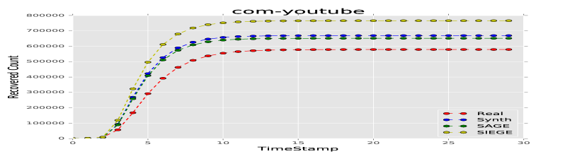
(d)

Figure 3. (a,c) represents the infected population count of the epidemic, wherein we see the expected spike patterns are present in both of the datasets and their synthetic counterpart. Overall $SAGE$ stays closest to the real world, followed by $Synth$ and then $SIEGE$. This is expected as $SIEGE$ has additional links created owing to its edge bridge augmentation which provides more route for the infection to spread to new nodes and so it would stray from the real world in terms of absolute count. (b,d) represents the recovered population where it can be seen that $SAGE$ outperforms $Synth$ and $SIEGE$. Overall $SAGE$ maintains greater fidelity in terms of reaction to SIR epidemic.

Table 2. $SAGE$ outperforms baseline $Synth$ as well as $SIEGE$ for collaboration networks in terms of matching upto the $Real$ world topology, while for autonomous networks $SIEGE$ does the same. Both however, in almost all cases outperforms the baseline $Synth$. All of them are improvements on DEG which would give N/A in all these cases.$EB_{Count}$ captures edge bridge count

Global  Clustering  Coefficient
Topology	$EB_{Count}$	$cf_{Real}$	$cf_{Synth}$	$cf_{sage}$	$cf_{siege}$
egoFacebook	75	0.60554	0.17150	0.13534	0.13324
caGrQc	1142	0.52960	0.64378	0.48748	0.37972
caHepTh	2030	0.47143	0.59098	0.46831	0.22546
oregon010331	3799	0.29700	0.82920	0.68256	0.47830
oregon010407	3848	0.29210	0.64214	0.68730	0.47380
oregon010414	3853	0.29540	0.82926	0.67889	0.47723
oregon010421	3855	0.29680	0.82903	0.68167	0.47891
oregon010428	3844	0.29400	0.82948	0.68310	0.47353
oregon020331	3274	0.50090	0.79330	0.63260	0.49710
oregon020407	3332	0.34630	0.79262	0.63577	0.49019
oregon020414	3316	0.34730	0.73276	0.63130	0.49460
oregon020421	3294	0.34960	0.79208	0.63152	0.49562
oregon020428	3283	0.34720	0.79165	0.63136	0.49750
oregon020505	3282	0.34610	0.79305	0.63379	0.49737
oregon020512	3296	0.34650	0.79243	0.63581	0.50218
oregon020519	3320	0.34840	0.79332	0.63709	0.49836
oregon020526	3351	0.41430	0.78936	0.63203	0.49721
email-Enron	10714	0.49700	0.54747	0.44578	0.36447
loc-gowalla	54351	0.23670	0.51262	0.40931	0.33317
loc-brightkite	23155	0.17230	0.59817	0.47045	0.33137
com-amazon	312191	0.39670	0.42287	0.40765	0.36733
com-dblp	47103	0.63240	0.48473	0.42230	0.36637
com-youtube	667090	0.08080	0.73160	0.58609	0.33239
as-skitter	232141	0.25810	0.43069	0.34795	0.32145
com-liveJournal	821887	0.28427	0.38987	0.28572	0.25469

6. Results and Discussions

For want of space all the graphical plots cannot be shown. We present the results for as-skitter, com-LiveJournal and oregon010428 primarily.

• How similar are triadic closures at the node level?

  • Clustering Coefficient Distribution: As can be seen in Figure 4 (a,b,c), the clustering coefficient distribution for Synth , SAGE and SIEGE follows the trend of the real world. The variance as the node degree increases is comparatively lesser for the three synthetic topologies as opposed to the real world network. The global clustering coefficient values presented in Table 2, that is, $CF_{Synth}$, $CF_{SAGE}$, $CF_{SIEGE}$ consistently showed a decrement in value for any given dataset. This is a direct consequence of the fact that SAGE and SIEGE allows for more single edge creation that increases the total number of triples in the topology. In terms of actual values $CF_{SAGE}$ was closest to the real world collaboration topologies ca-Gr-Qc, com-amazon, com-liveJournal and ca-Hep-Th. For the autonomous systems based networks and location based OSN SIEGE clearly performed best.

• Can the models reproduce the reachability nature of the real world data?

  • Shortest Path Distribution: As can be seen in Figure 4 (d,e,f) the Synthetic topologies matches quite well with the real world topology. This was observed across all the datasets, except for the last seven large datasets in table 1 for which the all pair shortest path computation time bloated out and hence we cannot comment on them. So we show the results for oregon010331, oregon010414 in figure 4 (d,f) instead. The distributions are either unimodal or vaguely bimodal for the real world datasets. The synthetic topologies are unimodal. However, as stated earlier they still capture the trend.

• What about other clustering heuristics?

  • k-core vs core node distribution: The real world topologies tend to have more nodes participating in k-core when k is less. As k increases the total number of nodes participating tends to decrease. For all the twenty-five real world datasets,(A sample of which has been provided in Figure 4 (g,h,i)) this property was seen and the synthetic topologies captured this characteristics as well. Among the three synthetic generation algorithm SIEGE is performing better in general.

  • k-core vs core edge distribution: The k-core vs core participating edges distribution also matched well for all the datasets. The broad trend of more participating edges in less valued core was captured effectively by all the algorithms as evident in Figure 4 (j,k,l).

• Is there a power law?

  • Node Degree Distribution As shown in Figure 4 (m,n,o) the heavy tail power law distribution is maintained making these algorithms suitable for generating synthetic topologies imitating real world networks. A wide variance is observed even on a log-log scale at node degree axis for Synth which is our baseline, which stabilizes as the heavy tail is approached. This is not the case for SAGE and SIEGE . This trend seems to be consistent across all the datasets. SIEGE clearly outperforms Synth in all these datasets and captures the heavy tail very effectively as the node degree increases.

• Does the model shed light into the behavioral nature of graphs?

  • SIR Epidemiological Simulation Outcome We choose the disease transmission rate to be 0.3 and the recovery rate to be 0.5 for the population. As shown in Figure 3(a,c) this results in a spike in the total infected count before the epidemics starts dying out. SAGE stays closest to the real world followed by Synth followed by SIEGE . Figure 3(b,d) represents the recovered population count with SAGE performing better than the rest.

• What do we lose as we scale up?

  • Experimental evidence shows us we do not lose much in terms of conformity to the real world characteristics across all the datasets, except for the case of absolute values of the average clustering coefficient distribution. The global value maintains considerable fidelity as shown in Table 2. In this paper we are not specifically doing any study of the effect of variations of step size given any single dataset. Intuitively we expect accuracy to fall as step size increases.

7. Conclusion and Future work

Our work proposes stable algorithms for synthetic network generation at topological level. They are demonstrably better than current state-of-the-art algorithms. As our future work we plan to incorporate attribute values for the nodes as well as principles of homophily and diversity into the topology generation process. We hope that would create a richer synthetic dataset for the research community.

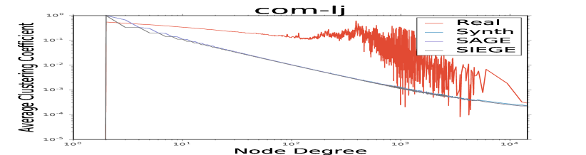
(a)

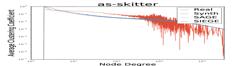
(b)

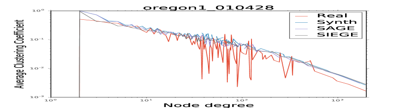
(c)

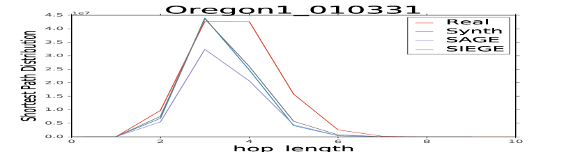
(d)

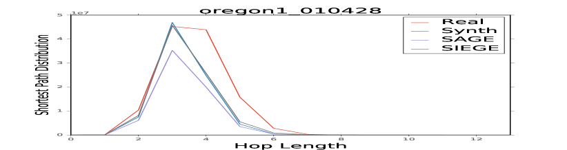
(e)

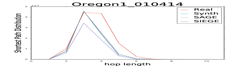
(f)

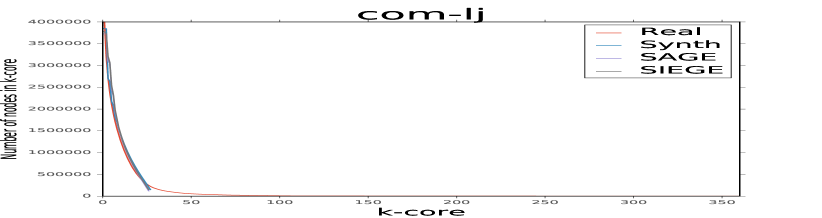
(g)

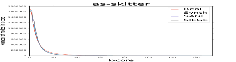
(h)

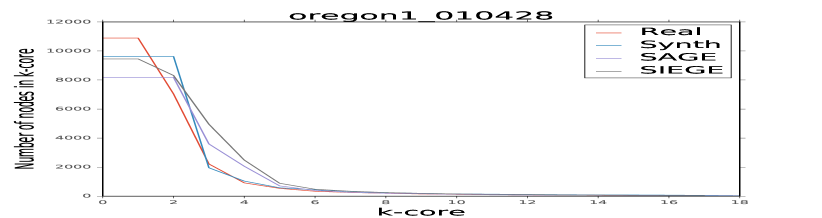
(i)

(j)

(k)

(l)

(m)

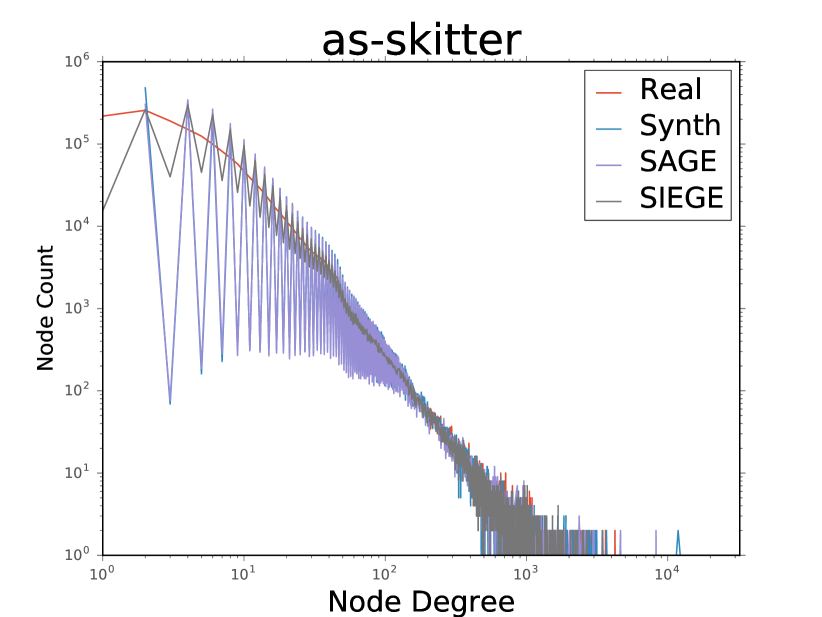
(n)

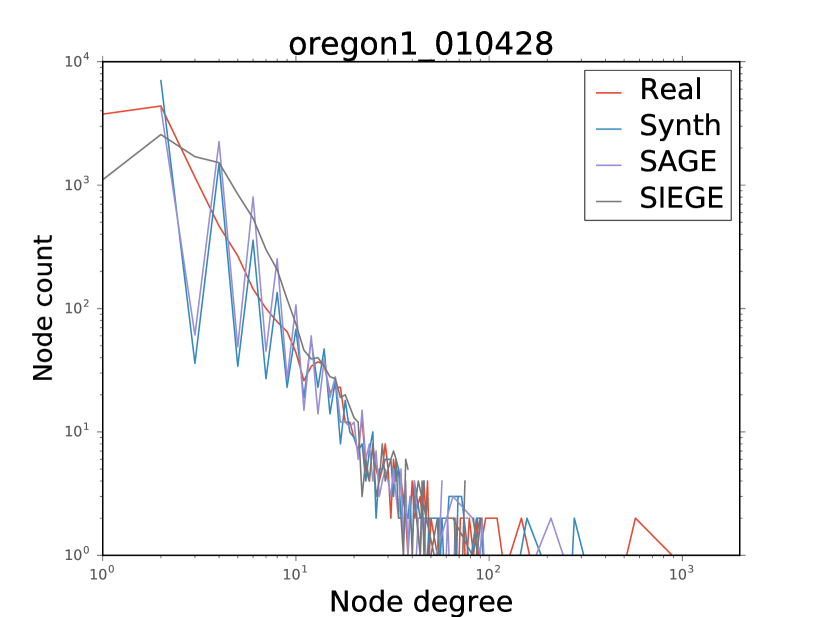
(o)

Figure 4. (a,b,c) represents the Local clustering coefficient distribution for dataset com-lj, as-skitter and Oregon010428 respectively, on a log-log scale. We can see the real network trend is broadly captured by all 3 models. (d,e,f) represents the hop-length distribution, which is either unimodal or bimodal for the real world. In all the datasets this characteristic is mimiced very well by our models. (g,h,i) represents k-core vs number of nodes participating in the core and (j,k,l) represents k-core vs number of edges participating in the core. In all six of them our models show encouraging stability. (m,n and o) represents the node degree distribution wherein our proposed model SIEGE outperforms the baseline Synth in all the cases. It is noted that in all these datasets the models produce stable results as opposed to the model DEG which would stall, making the outcomes in most of these scenarios null. Thus there is a significant improvement in stability from our approach.

References

- (1)
- Adamic and Huberman (2000) L. A. Adamic and B. A. Huberman. 2000. Comment to” Emergence of Scaling in Random Networks”(cond-mat/9910332). arXiv preprint cond-mat/0001459 (2000).
- Barabási and Albert (1999) A. Barabási and R. Albert. 1999. Emergence of scaling in random networks. science 286, 5439 (1999), 509–512.
- Barrett et al. (2009) C. L. Barrett, R. J. Beckman, M. Khan, VS. A. Kumar, M. V. Marathe, P. E. Stretz, T. Dutta, and B. Lewis. 2009. Generation and analysis of large synthetic social contact networks. In Winter Simulation Conference. Winter Simulation Conference, 1003–1014.
- Camacho et al. (2002) J. Camacho, R. Guimerà, and Luís A Nunes Amaral. 2002. Robust patterns in food web structure. Physical Review Letters 88, 22 (2002), 228102.
- Cho et al. (2011) E. Cho, S. A. Myers, and J. Leskovec. 2011. Friendship and mobility: user movement in location-based social networks. In Proceedings of the 17th ACM SIGKDD international conference on Knowledge discovery and data mining. ACM, 1082–1090.
- Ebel et al. (2002) H. Ebel, L. Mielsch, and S. Bornholdt. 2002. Scale-free topology of e-mail networks. Physical review E 66, 3 (2002), 035103.
- Erdös and Rényi (1960) P. Erdös and A. Rényi. 1960. On the evolution of random graphs. Publ. Math. Inst. Hung. Acad. Sci 5, 17-61 (1960), 43.
- Gleeson (2009) J. P. Gleeson. 2009. Bond percolation on a class of clustered random networks. Physical Review E 80, 3 (2009), 036107.
- Guelzim et al. (2002) N. Guelzim, S. Bottani, P. Bourgine, and F. Képès. 2002. Topological and causal structure of the yeast transcriptional regulatory network. Nature genetics 31, 1 (2002), 60–63.
- Guo et al. (2006) Q. Guo, T. Zhou, J. Liu, W. Bai, B. Wang, and M. Zhao. 2006. Growing scale-free small-world networks with tunable assortative coefficient. Physica A: Statistical Mechanics and its Applications 371, 2 (2006), 814–822.
- Guo and Kraines (2009) W. Guo and S. B. Kraines. 2009. A random network generator with finely tunable clustering coefficient for small-world social networks. In Computational Aspects of Social Networks, 2009. CASON’09. International Conference on. IEEE, 10–17.
- Heath and Parikh (2011) L. S. Heath and N. Parikh. 2011. Generating random graphs with tunable clustering coefficients. Physica A: Statistical Mechanics and its Applications 390, 23 (2011), 4577–4587.
- Holme and Kim (2002) P. Holme and B. J. Kim. 2002. Growing scale-free networks with tunable clustering. Physical review E 65, 2 (2002), 026107.
- Jeong et al. (2003) H. Jeong, Z. Néda, and A. Barabási. 2003. Measuring preferential attachment in evolving networks. EPL (Europhysics Letters) 61, 4 (2003), 567.
- Kermack and McKendrick (1927) W. O Kermack and A. G McKendrick. 1927. A contribution to the mathematical theory of epidemics. In Proceedings of the Royal Society of London A: mathematical, physical and engineering sciences, Vol. 115. The Royal Society, 700–721.
- Kleinberg et al. (1999) J. M Kleinberg, R. Kumar, P. Raghavan, S. Rajagopalan, and A. S Tomkins. 1999. The web as a graph: measurements, models, and methods. In International Computing and Combinatorics Conference. Springer, 1–17.
- Klimt and Yang (2004) B. Klimt and Y. Yang. 2004. Introducing the Enron Corpus.. In CEAS.
- Kumar et al. (2000) R. Kumar, P. Raghavan, S. Rajagopalan, D Sivakumar, A. Tomkins, and E. Upfal. 2000. Stochastic models for the web graph. In Foundations of Computer Science, 2000. Proceedings. 41st Annual Symposium on. IEEE, 57–65.
- Leskovec et al. (2005) J. Leskovec, J. Kleinberg, and C. Faloutsos. 2005. Graphs over time: densification laws, shrinking diameters and possible explanations. In Proceedings of the eleventh ACM SIGKDD international conference on Knowledge discovery in data mining. ACM, 177–187.
- Leskovec et al. (2009) J. Leskovec, K. J. Lang, A. Dasgupta, and M. W. Mahoney. 2009. Community structure in large networks: Natural cluster sizes and the absence of large well-defined clusters. Internet Mathematics 6, 1 (2009), 29–123.
- Mantel (1907) W. Mantel. 1907. Problem 28. Wiskundige Opgaven 10, 60-61 (1907), 320.
- McAuley and Leskovec (2012) J. J. McAuley and J. Leskovec. 2012. Learning to Discover Social Circles in Ego Networks.. In NIPS, Vol. 2012. 548–56.
- McPherson et al. (2001) M. McPherson, L. Smith-Lovin, and J. M. Cook. 2001. Birds of a feather: Homophily in social networks. Annual review of sociology (2001), 415–444.
- Molloy and Reed (1995) M. Molloy and B. Reed. 1995. A critical point for random graphs with a given degree sequence. Random structures & algorithms 6, 2-3 (1995), 161–180.
- Nettleton (2015) D. F. Nettleton. 2015. Generating synthetic online social network graph data and topologies. In 3rd Workshop on Graph-based Technologies and Applications (Graph-TA), UPC, Barcelona, Spain, March.
- Newman (2009) M. EJ. Newman. 2009. Random graphs with clustering. Physical review letters 103, 5 (2009), 058701.
- Newman and Watts (1999) M. EJ. Newman and D. J. Watts. 1999. Renormalization group analysis of the small-world network model. Physics Letters A 263, 4 (1999), 341–346.
- Pérez-Rosés and Sebé (2015) H. Pérez-Rosés and F. Sebé. 2015. Synthetic generation of social network data with endorsements. Journal of Simulation 9, 4 (2015), 279–286.
- Price (1976) D. S. Price. 1976. A general theory of bibliometric and other cumulative advantage processes. Journal of the American society for Information science 27, 5 (1976), 292–306.
- Schank and Wagner (2004) T. Schank and D. Wagner. 2004. Approximating clustering-coefficient and transitivity. Universität Karlsruhe, Fakultät für Informatik.
- Schank and Wagner (2005) T. Schank and D. Wagner. 2005. Finding, counting and listing all triangles in large graphs, an experimental study. In International Workshop on Experimental and Efficient Algorithms. Springer, 606–609.
- Solomonoff and Rapoport (1951) R. Solomonoff and A. Rapoport. 1951. Connectivity of random nets. The bulletin of mathematical biophysics 13, 2 (1951), 107–117.
- Tarjan (1974) R. E. Tarjan. 1974. A note on finding the bridges of a graph. Inform. Process. Lett. 2, 6 (1974), 160–161.
- Wang et al. (2008) J. Wang, L. Rong, and L. Zhang. 2008. Evolving small-world networks of the local world with tunable clustering. In 2008 ISECS International Colloquium on Computing, Communication, Control, and Management, Vol. 2. IEEE, 369–373.
- Watts and Strogatz (1998) D. J. Watts and S. H. Strogatz. 1998. Collective dynamics of ‘small-world’networks. nature 393, 6684 (1998), 440–442.
- White et al. (1986) J. G White, E. Southgate, J Nichol Thomson, and S. Brenner. 1986. The structure of the nervous system of the nematode Caenorhabditis elegans. Philos Trans R Soc Lond B Biol Sci 314, 1165 (1986), 1–340.
- Yang and Leskovec (2015) J. Yang and J. Leskovec. 2015. Defining and evaluating network communities based on ground-truth. Knowledge and Information Systems 42, 1 (2015), 181–213.