Weakly-normal basis vector fields in RKHS with an application to shape Newton methods

Abstract

We construct a space of vector fields that are normal to differentiable curves in the plane. Its basis functions are defined via saddle point variational problems in reproducing kernel Hilbert spaces (RKHSs). First, we study the properties of these basis vector fields and show how to approximate them. Then, we employ this basis to discretise shape Newton methods and investigate the impact of this discretisation on convergence rates.

AMS classification: 49Q10, 49M15, 93B40, 65Dxx

1 Introduction

Shape optimisation studies how to design a domain $\Omega$ such that a shape functional $J$ is minimised. Shape optimization problems arise naturally in numerous industrial applications. Just to mention a few examples, shape optimization can be used to improve the design of electrodes [4], bridges [2], breakwaters [21], optical lenses [24], airplane components [25], and 3D printers [7]. In light of its wide range of applications, it is not a surprise that several commercial products offer shape optimisation features.

Shape optimisation problems are inherently infinite dimensional. Therefore, any numerical shape optimisation algorithm must rely on a discretisation of the space of shapes. Additionally, shape optimization problems are in most instances nonconvex. Therefore, numerical shape optimisation software commonly relies on iterative optimisation algorithms. In particular, in light of the large number of optimization parameters, it is advantageous to use optimization strategies that involve derivatives of the functional $J$, like steepest descent or Newton’s algorithm.

The derivative of $J$ with respect to perturbations of $\Omega$ is called its shape derivative and its technical definition depends on how these domain perturbations are modeled. Historically, domain perturbations have been defined in terms of velocity flows or perturbations of the identity [9, 18, 31]. Recently, Allaire et al. [1] have introduced domain perturbations in terms of Hamilton-Jacobi equations. These definitions lead to the same formulas for first-order shape derivatives, but differ for second-order ones. The equivalence of the three approaches for the first shape-derivative stems from the fact that each approach constructs domain perturbations from vector fields, and the Taylor series expansions of these constructions agree to first order. However, the second-order terms of these series do not match. Therefore, the corresponding shape Newton methods potentially deliver different shape updates.

Regardless of the definition used, both first- and second-order shape derivatives have a nontrivial kernel. For instance, shape derivatives are zero in the direction of vector fields that vanish on $\partial\Omega$. The Hadamard-Zolésio theorem and its second-order counterpart [23] provide a complete characterization of the kernel of shape derivatives. This information needs to be taken into account to prove convergence rates of shape Newton methods [32, 28] (because one must “quotient” the kernel from the search space) and has a direct consequence for numerical computations: if the discretisation of domain perturbations is not chosen carefully, the matrix that results by restricting the second-order shape derivative to the discrete trial space may fail to be positive definite (it is usually positive semi-definite). In particular, the basis vector fields used to discretise domain perturbations must necessarily have nonvanishing normal component on the boundary of $\Omega$.

Our goal is to construct basis vector fields that are normal to a given boundary $\partial\Omega$ and that have good approximation properties. The literature contains articles that address this issue and rely on vector fields with this geometric feature. In [14, 13, 16], the authors consider star-shaped domains whose parametrization formula is known analytically and construct the basis vector fields using this parametrization. This approach is at the same time ideal for and limited to shape optimization problems for which all computations can be restricted to the boundary $\partial\Omega$, because the basis vector fields constructed in [14, 13, 16] are defined only on $\partial\Omega$. To restrict all computations to the boundary, the domain $\Omega$ must satisfy certain regularity requirements, and if the shape functional $J$ is constrained to a boundary value problem, its solution must also be sufficiently smooth. If these conditions are not fulfilled, restricting all computations to $\partial\Omega$ is not possible, and one needs to employ basis vector fields whose support has nonzero measure. In practice, it is not difficult to construct such vector fields replacing $\Omega$ with a triangulation and using finite elements [29, 30]. However, the approximation properties of the constructed space are unclear, and it is difficult to understand whether the Newton updates are well-defined in the zero mesh-width limit.

In our work, we use reproducing kernel Hilbert spaces (RKHSs) to define a class of basis vector fields that are weakly-normal to the boundary of a domain $\Omega$ and whose support has nonzero measure. We use the term weakly-normal because this geometric property is enforced with the help of saddle point variational problems. This approach allows us to ensure that the resulting vector fields are linearly independent and normal to the shape boundary $\partial\Omega$. Therefore, they can be used to formulate discrete shape Newton methods. Moreover, these vector fields span a dense subset of the space of normal vector fields, and it is possible to analyse the error between exact and approximate shape Newton updates.

For simplicity, we restrict the exposition to the two dimensional case. However, the approach can be adapted to higher dimensions, although the implementation aspects may become more challenging.

2 Normal vector fields in RKHS

2.1 RKHSs, Cartesian products, and trace spaces

We begin with some basic definitions of reproducing kernels.

Definition 2.1.

Let $\mathcal{X}\subset{\mathbf{R}}^{2}$ be an arbitrary set. A function $\mathsf{k}:\mathcal{{\cal X}}\times{\cal X}\to{\mathbf{R}}$ is called reproducing kernel for the Hilbert space $\left({\cal H}(\mathcal{X}),(\cdot,\cdot)_{\cal H}\right)$ of functions $f:{\cal X}\to{\mathbf{R}}$, if

1. $\mathsf{k}({\mathbf{x}},\cdot)\in{\cal H}({\cal X})$ for every ${\mathbf{x}}\in\mathcal{X}$,

2. $(\mathsf{k}({\mathbf{x}},\cdot),f)_{{\cal H}}=f({\mathbf{x}})$ for every ${\mathbf{x}}\in\mathcal{X}$ and every $f\in{\cal H}({\cal X})$.

Definition 2.2.

A kernel $\mathsf{k}:{\cal X}\times{\cal X}\to{\mathbf{R}}$ is said to be positive-definite on ${\cal X}$ if, for every finite subset of pairwise distinct points $\{{\mathbf{x}}_{i}\}_{i=1}^{n}\subset{\cal X}$, the matrix $(\mathsf{k}({\mathbf{x}}_{i},{\mathbf{x}}_{j}))_{i,j=1}^{n}$ is positive-definite.

Definition 2.3.

A kernel $\mathsf{k}:{\cal X}\times{\cal X}\to{\mathbf{R}}$ is said to be symmetric if

$$\mathsf{k}({\mathbf{x}},{\mathbf{y}})=\mathsf{k}({\mathbf{y}},{\mathbf{x}})\quad\text{for all }{\mathbf{x}},{\mathbf{y}}\in{\cal X}\,.$$

The main reason to consider symmetric positive-definite reproducing kernels is that they can be used to define certain Hilbert Spaces.

Theorem 2.4.

To a positive-definite and symmetric kernel $\mathsf{k}:{\cal X}\times{\cal X}\to{\mathbf{R}}$ defined on an arbitrary set ${\cal X}\subset{\mathbf{R}}^{2}$ corresponds a unique reproducing kernel Hilbert space $({\cal H}({\cal X}),(\cdot,\cdot)_{{\cal H}})$ (RKHS), which is called native space of $\mathsf{k}$. Note that $(\cdot,\cdot)_{{\cal H}}$ depends on $\mathsf{k}$.

There is a variety of symmetric positive-definite reproducing kernels [34] (each tailored to specific applications). In this work, we are particularly interested in Wendland kernels with compact support because, for applications in shape optimisation, compact support is a useful (it implies sparsity of the discretised shape Hessian) and sometimes necessary (when part of the domain is not “free to move” [22]) feature . In the next example, we list three Wendland kernels and recall their native spaces.

Example 2.5.

Classical examples of positive-definite kernels can be found in [34]. In this work, we are particularly interested in

(1) $$\mathsf{k}^{\sigma}_{4}(x,y)\coloneqq\left(1-\frac{|x-y|}{\sigma}\right)_{+}^{4}\left(4\frac{|x-y|}{\sigma}+1\right),\quad\sigma>0,$$

where

$$(\cdot)_{+}:{\mathbf{R}}\to{\mathbf{R}}^{+}_{0}\,,\quad x\mapsto(x)_{+}\coloneqq\max(0,x)\,.$$

When $\sigma=1$, Eq. 1 is the lowest order Wendland kernel with compact support that is positive-definite on ${\mathbf{R}}^{d}$ (for $d\leq 3$) and is of class $C^{2}$. When ${\cal X}={\mathbf{R}}^{2}$, its native space is $H^{2.5}({\mathbf{R}}^{2})$ [34, p. 160, Thm. 10.35]. When ${\cal X}=\Omega$ is a bounded smooth domain, its native space is $H^{2.5}(\Omega)$ (because every function $f\in{\cal H}(\Omega)$ can be extended to a function $\tilde{f}\in{\cal H}({\mathbf{R}}^{2})=H^{2.5}({\mathbf{R}}^{2})$ [34, p. 169, Thm. 10.46]). Similar properties can be proved for the $C^{4}$-kernel $\mathsf{k}^{\sigma}_{6}$ and the $C^{6}$-kernel $\mathsf{k}^{\sigma}_{8}$, which are given by [34],

(2) $$\mathsf{k}^{\sigma}_{6}(x,y) \coloneqq\frac{1}{3}\left(1-\frac{|x-y|}{\sigma}\right)_{+}^{6}\left(35\frac{|x-y|^{2}}{\sigma^{2}}+18\frac{|x-y|}{\sigma}+3\right),$$

(3) $$\mathsf{k}^{\sigma}_{8}(x,y) \coloneqq\left(1-\frac{|x-y|}{\sigma}\right)_{+}^{8}\left(32\frac{|x-y|^{3}}{\sigma^{3}}+25\frac{|x-y|^{2}}{\sigma^{2}}+8\frac{|x-y|}{\sigma}+1\right)\,,$$

respectively. Their corresponding native spaces in dimension two are $H^{3.5}({\mathbf{R}}^{2})$ and $H^{4.5}({\mathbf{R}}^{2})$, respectively [34, p. 160, Thm. 10.35].

Scalar reproducing kernels can be used to define Hilbert spaces of vector valued functions, too [11, Lemma 3.6].

Proposition 2.6.

The Cartesian product $[{\cal H}({\cal X})]^{2}\coloneqq{\cal H}({\cal X})\times{\cal H}({\cal X})$ of a RKHS ${\cal H}({\cal X})$ (with reproducing kernel $\mathsf{k}$) is itself a RKHS. Its (matrix valued) reproducing kernel is $\mathsf{k}(\cdot,\cdot){\mathbf{I}}$, where ${\mathbf{I}}\in{\mathbf{R}}^{2}$ denotes the identity matrix. Henceforth, we denote by $(\cdot,\cdot)_{[{\cal H}]^{2}}$ the (canonical) inner product of $[{\cal H}({\cal X})]^{2}$.

Next, we describe how to construct RKHSs on boundaries of bounded subdomains of ${\mathbf{R}}^{2}$. Let $\mathsf{k}$ be a positive-definite kernel on ${\mathbf{R}}^{2}$, and let ${\cal H}({\mathbf{R}}^{2})$ be its native space. Let $\Omega\subset{\mathbf{R}}^{2}$ be a nonempty, bounded, open and smooth set (e.g. $C^{1}$). We denote by $\boldsymbol{\nu}$ and $\boldsymbol{\tau}$ the unit normal and unit tangential vector fields along $\partial\Omega$.

The restriction of $\mathsf{k}$ onto $\partial\Omega$ defines a positive-definite kernel $\mathsf{k}|_{\partial\Omega}$, which uniquely characterises the RKHS [34, p.169]

(4) $${\cal H}(\partial\Omega)=\{f|_{\partial\Omega}:\;f\in{\cal H}({\mathbf{R}}^{2})\}\,.$$

Similarly, it is possible to define the space of vector fields restricted onto $\partial\Omega$ by

(5) $$[\mathcal{H}(\partial\Omega)]^{2}=\{{\mathbf{f}}|_{\partial\Omega}:\;{\mathbf{f}}\in[\mathcal{H}({\mathbf{R}}^{2})]^{2}\}.$$

The next example identifies the space $\mathcal{H}(\partial\Omega)$ for the kernel Eq. 1.

Example 2.7.

The native space of the restriction onto $\partial\Omega$ of the Wendland kernel $\mathsf{k}_{4}^{\sigma}$ (with $\sigma$ fixed) is $H^{2}(\partial\Omega)$. This follows from ${\cal H}({\mathbf{R}}^{2})=H^{2.5}({\mathbf{R}}^{2})$ and the standard Sobolev trace theorem.

We conclude this section by defining the RKHS of normal and tangential vector fields:

(6) $$[{\cal H}(\partial\Omega)]^{2}_{\boldsymbol{\nu}} \coloneqq\{{\mathbf{f}}\in[\mathcal{H}({\mathbf{R}}^{2})]^{2}:\;{\mathbf{f}}\cdot\boldsymbol{\tau}=0\quad\text{ on }\partial\Omega\}\,,$$

(7) $$[{\cal H}(\partial\Omega)]^{2}_{\boldsymbol{\tau}} \coloneqq\{{\mathbf{f}}\in[\mathcal{H}({\mathbf{R}}^{2})]^{2}:\;{\mathbf{f}}\cdot\boldsymbol{\nu}=0\quad\text{ on }\partial\Omega\}.$$

2.2 Weakly-normal basis functions

In this section, we introduce a novel class of normal vector fields. We begin with the following assumption on the reproducing kernel $\mathsf{k}$.

Assumption 2.8.

Let $k\geq 1$ be an integer and let $\partial\Omega$ be of class $C^{k+1}$. We assume that $\mathsf{k}:{\mathbf{R}}^{2}\times{\mathbf{R}}^{2}\to{\mathbf{R}}$ is a symmetric positive-definite kernel on ${\mathbf{R}}^{2}$ with the property

(8) $$\mathsf{k}({\mathbf{x}},{\mathbf{x}})=1\quad\text{for all }{\mathbf{x}}\in\partial\Omega\,.$$

We assume that for every ${\mathbf{x}}\in{\mathbf{R}}^{2}$ we have $\mathsf{k}({\mathbf{x}},\cdot)\in C^{k}({\mathbf{R}}^{2})$. Furthermore, we assume that there is a constant $c_{\Omega}>0$, such that for every $\phi\in C^{k}(\partial\Omega)$ and every $f\in{\cal H}(\partial\Omega)$,

(9) $$\phi f\in{\cal H}(\partial\Omega)\quad\text{and}\quad\|\phi f\|_{{\cal H}}\leq c_{\Omega}\|\phi\|_{C^{k}(\partial\Omega)}\|f\|_{{\cal H}}.$$

Finally, we assume that the constant function $1:\partial\Omega\to{\mathbf{R}}$ belongs to ${\cal H}(\partial\Omega)$ and, for simplicity, that the support of $\mathsf{k}$ is connected.

Example 2.9.

The kernels $\mathsf{k}^{\sigma}_{4},\mathsf{k}^{\sigma}_{6}$ and $\mathsf{k}^{\sigma}_{8}$ satisfy 2.8 for $k=2,3,4$, respectively.

Remark 2.10.

Property Eq. 9 implies that $C^{k}(\partial\Omega)\subset{\cal H}(\partial\Omega)$ (by Eq. 9), and that $[{\cal H}(\partial\Omega)]^{2}=[{\cal H}(\partial\Omega)]^{2}_{\boldsymbol{\nu}}\oplus[{\cal H}(\partial\Omega)]^{2}_{\boldsymbol{\tau}}$ (because every vector field ${\mathbf{v}}\in[{\cal H}(\partial\Omega)]^{2}$ can be decomposed into ${\mathbf{v}}=({\mathbf{v}}\cdot\boldsymbol{\nu})\boldsymbol{\nu}+({\mathbf{v}}\cdot\boldsymbol{\tau})\boldsymbol{\tau}$ on $\partial\Omega$).

Definition 2.11.

For a point ${\mathbf{x}}\in\partial\Omega$, let $({\mathbf{r}}_{\mathbf{x}},p_{\mathbf{x}})\in[{\cal H}(\partial\Omega)]^{2}\times{\cal H}(\partial\Omega)$ be the solution of

(10a) $$({\mathbf{r}}_{\mathbf{x}},\boldsymbol{\varphi})_{[{\cal H}]^{2}}+(\boldsymbol{\varphi}\cdot\boldsymbol{\tau},p_{\mathbf{x}})_{\mathcal{H}} =\boldsymbol{\nu}({\mathbf{x}})\cdot\boldsymbol{\varphi}({\mathbf{x}}) \text{ for all }\boldsymbol{\varphi}\in[\mathcal{H}(\partial\Omega)]^{2},$$

(10b) $$\;({\mathbf{r}}_{\mathbf{x}}\cdot\boldsymbol{\tau},\psi)_{\mathcal{H}} =0 \text{ for all }\psi\in\mathcal{H}(\partial\Omega)\,.$$

The function ${\mathbf{r}}_{\mathbf{x}}$ is the weakly-normal basis function associated with ${\mathbf{x}}$.

To show that Definition 2.11 makes sense, we need to prove that Eq. 10 admits a unique and stable solution. This is done in Lemma 2.14, which in turn relies on Lemma 2.12. Before showing Lemma 2.12, we introduce the following notation: henceforth we denote by ${\mathbf{e}}_{i},i=1,2,$ the canonical basis of ${\mathbf{R}}^{2}$ and use the norm

(11) $$\|{\mathbf{f}}\|_{C^{k}}\coloneqq\sqrt{\|{\mathbf{f}}\cdot{\mathbf{e}}_{1}\|_{C^{k}}^{2}+\|{\mathbf{f}}\cdot{\mathbf{e}}_{2}\|_{C^{k}}^{2}}\quad\text{for all }{\mathbf{f}}\in C^{k}({\mathbf{R}}^{2},{\mathbf{R}}^{2})\,.$$

Lemma 2.12.

The operator $B:[\mathcal{H}(\partial\Omega)]^{2}\rightarrow\mathcal{H}(\partial\Omega)^{*}$ defined by $\boldsymbol{\varphi}\mapsto(\boldsymbol{\varphi}\cdot\boldsymbol{\tau},\cdot)_{\mathcal{H}}$ is surjective. Moreover,

(12) $$\|B^{*}\psi\|_{([{\cal H}]^{2})^{*}}\geq\frac{\|\psi\|_{{\cal H}}}{c_{\Omega}\|\boldsymbol{\tau}\|_{C^{k}}}\quad\text{ for all }\psi\in{\cal H}(\partial\Omega)\,.$$

Proof 2.13.

To show that $B$ is surjective, let $f\in{\cal H}(\partial\Omega)^{*}$. By the Riesz representation theorem, there is a function $\eta_{f}\in{\cal H}(\partial\Omega)$ that satisfies $f(\psi)=(\eta_{f},\psi)_{\cal H}$ for all $\psi\in{\cal H}(\partial\Omega)$. Since the function $\boldsymbol{\varphi}\coloneqq\eta_{f}\boldsymbol{\tau}\in[\mathcal{H}(\partial\Omega)]^{2}$ satisfies $B\boldsymbol{\varphi}=f$, the operator $B$ is surjective. To verify Eq. 12, first note that inequality Eq. 9 implies $\|\boldsymbol{\tau}\psi\|_{[{\cal H}]^{2}}\leq c_{\Omega}\|\boldsymbol{\tau}\|_{C^{k}}\|\psi\|_{{\cal H}}$ for every $\psi\in{\cal H}(\partial\Omega)$. Thus,

$$\|B^{*}\psi\|_{([{\cal H}]^{2})^{*}}=\sup_{\begin{subarray}{c}\boldsymbol{\varphi}\in[{\cal H}(\partial\Omega)]^{2}\\ \|\boldsymbol{\varphi}\|_{[{\cal H}]^{2}}=1\end{subarray}}|(\boldsymbol{\tau}\cdot\boldsymbol{\varphi},\psi)_{{\cal H}}| \geq\left(\frac{\boldsymbol{\tau}\cdot(\boldsymbol{\tau}\psi)}{\|\boldsymbol{\tau}\psi\|_{[{\cal H}]^{2}}},\psi\right)_{{\cal H}}\geq\frac{\|\psi\|_{{\cal H}}}{c_{\Omega}\|\boldsymbol{\tau}\|_{C^{k}}}\,.$$

Lemma 2.14.

Let ${\mathbf{x}}\in\partial\Omega$. The saddle point problem Eq. 10 admits a unique solution, which satisfies

(13) $$\|{\mathbf{r}}_{\mathbf{x}}\|_{[{\cal H}]^{2}}\leq\frac{1}{\|\boldsymbol{\nu}\|_{[{\cal H}]^{2}}}\,,\quad\text{and}\quad\|p_{\mathbf{x}}\|_{{\cal H}}\leq\frac{2c_{\Omega}\|\boldsymbol{\tau}\|_{C^{k}}}{\|\boldsymbol{\nu}\|_{[{\cal H}]^{2}}}\,.$$

Proof 2.15.

Since $B$ is surjective and $(\cdot,\cdot)_{[{\cal H}]^{2}}$ is an inner product, existence and uniqueness follow from the classical result [5, Thm 4.2.1, p.224]. The continuity estimates Eq. 13 follow from [5, Thm 4.2.3, p.228], Eq. 12, and the estimate

(14) $$\sup_{\begin{subarray}{c}\boldsymbol{\varphi}\in[{\cal H}]^{2},\\ \|\boldsymbol{\varphi}\|_{[{\cal H}]^{2}}=1\end{subarray}}|\boldsymbol{\nu}({\mathbf{x}})\cdot\boldsymbol{\varphi}({\mathbf{x}})|\leq\frac{|\boldsymbol{\nu}({\mathbf{x}})\cdot\boldsymbol{\nu}({\mathbf{x}})|}{\|\boldsymbol{\nu}\|_{[{\cal H}]^{2}}}\leq 1/\|\boldsymbol{\nu}\|_{[{\cal H}]^{2}}\,.$$

Note that $1\in{\cal H}(\partial\Omega)$ by 2.8, and thus $\boldsymbol{\nu}\in[{\cal H}(\partial\Omega)]^{2}$.

The following remark provides an alternative definition of the function ${\mathbf{r}}_{\mathbf{x}}$.

Remark 2.16.

Let ${\mathbf{x}}\in\partial\Omega$. The solution ${\mathbf{r}}_{\mathbf{x}}\in[{\cal H}(\partial\Omega)]^{2}$ of Eq. 10 is the unique minimiser of

(15) $$\min_{\begin{subarray}{c}\boldsymbol{\varphi}\in[{\cal H}(\partial\Omega)]^{2},\\ \boldsymbol{\varphi}\cdot\boldsymbol{\tau}=0\text{ on }\partial\Omega\end{subarray}}\frac{1}{2}\|\boldsymbol{\varphi}\|_{[{\cal H}]^{2}}^{2}-\boldsymbol{\nu}({\mathbf{x}})\cdot\boldsymbol{\varphi}({\mathbf{x}}).$$

Proof 2.17.

By differentiating the Lagrangian functional

(16) $${\cal L}:[{\cal H}(\partial\Omega)]^{2}\times{\cal H}(\partial\Omega)\to{\mathbf{R}}\,,\quad(\boldsymbol{\varphi},\psi)\mapsto\frac{1}{2}\|\boldsymbol{\varphi}\|_{[{\cal H}]^{2}}^{2}-\boldsymbol{\nu}({\mathbf{x}})\cdot\boldsymbol{\varphi}({\mathbf{x}})+(\boldsymbol{\varphi}\cdot\boldsymbol{\tau},\psi)_{\cal H}\,,$$

it is easy to see that equations Eq. 10 are the first order optimality conditions of Eq. 15. This is the so-called Lagrange multiplier rule. Since $\boldsymbol{\varphi}\mapsto 1/2\|\boldsymbol{\varphi}\|_{[{\cal H}]^{2}}^{2}-\boldsymbol{\nu}({\mathbf{x}})\cdot\boldsymbol{\varphi}({\mathbf{x}})$ is a convex and coercive functional, ${\mathbf{r}}_{\mathbf{x}}$ is a minimiser of Eq. 15, where $({\mathbf{r}}_{\mathbf{x}},p_{\mathbf{x}})$ is a solution of the saddle point equation Eq. 10.

In the next theorem, we analyse in details the properties of ${\mathbf{r}}_{\mathbf{x}}$ and show that, in general, ${\mathbf{r}}_{\mathbf{x}}$ is neither $\boldsymbol{\nu}(\cdot)\mathsf{k}({\mathbf{x}},\cdot)$ nor $\boldsymbol{\nu}(\cdot)$. To facilitate the interpretation, in Fig. 1 we include some plots of the function ${\mathbf{r}}_{\mathbf{x}}$.

Theorem 2.18.

Let ${\mathbf{x}}\in\partial\Omega$. The solution $({\mathbf{r}}_{\mathbf{x}},p_{\mathbf{x}})$ of Eq. 10 has the following properties.

1. ${\mathbf{r}}_{\mathbf{x}}\in[{\cal H}(\partial\Omega)]^{2}_{\boldsymbol{\nu}}$.

2. $\|{\mathbf{r}}_{\mathbf{x}}\|_{[{\cal H}]^{2}}\leq 1$.

3. $\|{\mathbf{r}}_{\mathbf{x}}\|_{[{\cal H}]^{2}}>0$, and the surface measure of $\operatorname{supp}({\mathbf{r}}_{\mathbf{x}})$ is strictly greater than zero.

4. The equality $\|{\mathbf{r}}_{\mathbf{x}}\|_{[{\cal H}]^{2}}=1$ holds if and only if $\partial\Omega\cap\operatorname{supp}({\mathbf{r}}_{\mathbf{x}})$ is a straight segment. In particular, $({\mathbf{r}}_{\mathbf{x}},p_{\mathbf{x}})=(\mathsf{k}({\mathbf{x}},\cdot)\boldsymbol{\nu}({\mathbf{x}}),0)$.

5. $({\mathbf{r}}_{\mathbf{x}},\boldsymbol{\nu})_{[{\cal H}]^{2}}=1$ and $\|\boldsymbol{\nu}\|_{[{\cal H}]^{2}}\|{\mathbf{r}}_{\mathbf{x}}\|_{[{\cal H}]^{2}}=1$. In particular, if $\|\boldsymbol{\nu}\|_{[{\cal H}]^{2}}=1$, then $\partial\Omega$ is a straight segment.

6. If $\partial\Omega\cap\operatorname{supp}({\mathbf{r}}_{\mathbf{x}})$ is not a straight segment, then

   (17) $${\mathbf{r}}_{\mathbf{x}}\neq\boldsymbol{\nu}(\cdot)\mathsf{k}({\mathbf{x}},\cdot)\quad\text{and}\quad{\mathbf{r}}_{\mathbf{x}}\neq\boldsymbol{\nu}\,.$$

7. The basis functions ${\mathbf{r}}_{\mathbf{x}},{\mathbf{r}}_{\mathbf{y}}$ associated with the points ${\mathbf{x}},{\mathbf{y}}\in\partial\Omega$ satisfy

   (18) $${\mathbf{r}}_{{\mathbf{x}}}({\mathbf{y}})\cdot\boldsymbol{\nu}({\mathbf{y}})={\mathbf{r}}_{{\mathbf{y}}}({\mathbf{x}})\cdot\boldsymbol{\nu}({\mathbf{x}}).$$

   Moreover, for each ${\mathbf{x}}\in\partial\Omega$ there is a neighborhood $U_{\mathbf{x}}$ of ${\mathbf{x}}$ such that ${\mathbf{r}}_{\mathbf{x}}({\mathbf{y}})\cdot\boldsymbol{\nu}({\mathbf{y}})>0$ for all ${\mathbf{y}}\in U_{\mathbf{x}}$.

Proof 2.19.

Item a follows from Eq. 10b, because ${\mathbf{r}}_{\mathbf{x}}({\mathbf{y}})\cdot\boldsymbol{\tau}({\mathbf{y}})=({\mathbf{r}}_{\mathbf{x}}\cdot\boldsymbol{\tau},\mathsf{k}({\mathbf{y}},\cdot))_{\cal H}=0$ for every ${\mathbf{y}}\in\partial\Omega$.

To show Item b, note that choosing $\boldsymbol{\varphi}={\mathbf{r}}_{\mathbf{x}}$ in Eq. 10a gives

(19) $$\|{\mathbf{r}}_{\mathbf{x}}\|_{[{\cal H}]^{2}}^{2}={\mathbf{r}}_{\mathbf{x}}({\mathbf{x}})\cdot\boldsymbol{\nu}({\mathbf{x}})\leq|{\mathbf{r}}_{\mathbf{x}}({\mathbf{x}})|=\sqrt{|{\mathbf{r}}_{\mathbf{x}}({\mathbf{x}})\cdot{\mathbf{e}}_{1}|^{2}+|{\mathbf{r}}_{\mathbf{x}}({\mathbf{x}})\cdot{\mathbf{e}}_{2}|^{2}}.$$

The reproducing kernel property of $\mathsf{k}$ and Eq. 8 imply

(20) $$\|\mathsf{k}({\mathbf{x}},\cdot)\|_{{\cal H}}^{2}=(\mathsf{k}({\mathbf{x}},\cdot),\mathsf{k}({\mathbf{x}},\cdot))_{{\cal H}}=\mathsf{k}({\mathbf{x}},{\mathbf{x}})=1\,.$$

Therefore, by the reproducing kernel property of $\mathsf{k}$ and Cauchy-Schwarz inequality,

(21) $$|{\mathbf{r}}_{\mathbf{x}}({\mathbf{x}})\cdot{\mathbf{e}}_{i}|=|(\mathsf{k}({\mathbf{x}},\cdot),{\mathbf{r}}_{\mathbf{x}}\cdot{\mathbf{e}}_{i})_{{\cal H}}|\leq\|\mathsf{k}({\mathbf{x}},\cdot)\|_{{\cal H}}\|{\mathbf{r}}_{\mathbf{x}}\cdot{\mathbf{e}}_{i}\|_{{\cal H}}=\|{\mathbf{r}}_{\mathbf{x}}\cdot{\mathbf{e}}_{i}\|_{{\cal H}}\,,$$

and thus,

$$|{\mathbf{r}}_{\mathbf{x}}({\mathbf{x}})|^{2}=|{\mathbf{r}}_{\mathbf{x}}({\mathbf{x}})\cdot{\mathbf{e}}_{1}|^{2}+|{\mathbf{r}}_{\mathbf{x}}({\mathbf{x}})\cdot{\mathbf{e}}_{2}|^{2}\leq\|{\mathbf{r}}_{\mathbf{x}}\cdot{\mathbf{e}}_{1}\|_{{\cal H}}^{2}+\|{\mathbf{r}}_{\mathbf{x}}\cdot{\mathbf{e}}_{2}\|_{{\cal H}}^{2}=\|{\mathbf{r}}_{\mathbf{x}}\|_{[{\cal H}]^{2}}^{2}.$$

In light of Eq. 19, this yields

(22) $$\begin{split}\|{\mathbf{r}}_{\mathbf{x}}\|_{[{\cal H}]^{2}}^{2}\leq|{\mathbf{r}}_{\mathbf{x}}({\mathbf{x}})|\leq\|{\mathbf{r}}_{\mathbf{x}}\|_{[{\cal H}]^{2}},\end{split}$$

which, in turn, implies $\|{\mathbf{r}}_{\mathbf{x}}\|_{[{\cal H}]^{2}}\leq 1$.

To show Item c, suppose that ${\mathbf{r}}_{\mathbf{x}}=0$. Then, $p_{\mathbf{x}}=0$, because Eq. 10a implies that for any ${\mathbf{y}}\in\partial\Omega$

$$p_{\mathbf{x}}({\mathbf{y}}) =(\mathsf{k}({\mathbf{y}},\cdot),p_{\mathbf{x}})_{\mathcal{H}}=(\mathsf{k}({\mathbf{y}},\cdot)\boldsymbol{\tau}(\cdot)\cdot\boldsymbol{\tau}(\cdot),p_{\mathbf{x}})_{\mathcal{H}}$$

$$=\boldsymbol{\nu}({\mathbf{x}})\cdot\mathsf{k}({\mathbf{y}},{\mathbf{x}})\boldsymbol{\tau}({\mathbf{x}})-({\mathbf{r}}_{\mathbf{x}},\mathsf{k}({\mathbf{y}},\cdot)\boldsymbol{\tau}(\cdot))_{[{\cal H}]^{2}}=0\,.$$

However, $({\mathbf{r}}_{\mathbf{x}},p_{\mathbf{x}})=0$ does not satisfy Eq. 10a when the test function $\boldsymbol{\varphi}$ is $\boldsymbol{\varphi}=\mathsf{k}({\mathbf{x}},\cdot)\boldsymbol{\nu}(\cdot)\in[\mathcal{H}(\partial\Omega)]^{2}$. Finally, ${\mathbf{r}}_{\mathbf{x}}\neq\mathbf{0}$ implies that there is at least a point ${\mathbf{y}}\in\partial\Omega$ such that ${\mathbf{r}}_{\mathbf{x}}({\mathbf{y}})\neq 0$. Since ${\mathbf{r}}_{\mathbf{x}}$ is continuous on $\partial\Omega$, $\operatorname{supp}({\mathbf{r}}_{\mathbf{x}})$ contains an nonempty neighborhood $U_{\mathbf{y}}$ of ${\mathbf{y}}$.

To show Item d, let us first assume that $\|{\mathbf{r}}_{\mathbf{x}}\|_{[{\cal H}]^{2}}=1$. Then, equation Eq. 22 implies $|{\mathbf{r}}_{\mathbf{x}}({\mathbf{x}})|=\|{\mathbf{r}}_{\mathbf{x}}\|_{[{\cal H}]^{2}}$, and since

$$|{\mathbf{r}}_{\mathbf{x}}({\mathbf{x}})\cdot{\mathbf{e}}_{1}|^{2}+|{\mathbf{r}}_{\mathbf{x}}({\mathbf{x}})\cdot{\mathbf{e}}_{2}|^{2}=|{\mathbf{r}}_{\mathbf{x}}({\mathbf{x}})|^{2}=\|{\mathbf{r}}_{\mathbf{x}}\|_{[{\cal H}]^{2}}^{2}=\|{\mathbf{r}}_{\mathbf{x}}\cdot{\mathbf{e}}_{1}\|_{{\cal H}}^{2}+\|{\mathbf{r}}_{\mathbf{x}}\cdot{\mathbf{e}}_{2}\|_{{\cal H}}^{2}\,,$$

equation Eq. 21 becomes an equality (because $|{\mathbf{r}}_{\mathbf{x}}({\mathbf{x}})\cdot{\mathbf{e}}_{i}|\leq\|{\mathbf{r}}_{\mathbf{x}}\cdot{\mathbf{e}}_{i}\|_{{\cal H}}$). In particular, this implies that

$$|(\mathsf{k}({\mathbf{x}},\cdot),{\mathbf{r}}_{\mathbf{x}}\cdot{\mathbf{e}}_{i})_{{\cal H}}|=\|\mathsf{k}({\mathbf{x}},\cdot)\|_{{\cal H}}\|{\mathbf{r}}_{\mathbf{x}}\cdot{\mathbf{e}}_{i}\|_{{\cal H}}\,.$$

For nonzero vectors, Cauchy-Schwarz inequality becomes an equality if and only if the two vectors are linearly dependent. Since $\mathsf{k}({\mathbf{x}},\cdot)$ and ${\mathbf{r}}_{\mathbf{x}}$ are both nonzero, there is a nonzero vector $\boldsymbol{\alpha}\in{\mathbf{R}}^{2}$ such that ${\mathbf{r}}_{\mathbf{x}}(\cdot)=\mathsf{k}({\mathbf{x}},\cdot)\boldsymbol{\alpha}$ (in fact, $|\boldsymbol{\alpha}|=1$ because $|{\mathbf{r}}_{\mathbf{x}}({\mathbf{x}})|=1=\mathsf{k}({\mathbf{x}},{\mathbf{x}})$). This, combined with ${\mathbf{r}}_{\mathbf{x}}\in[{\cal H}(\partial\Omega)]^{2}_{\boldsymbol{\nu}}$ (see Item a), implies that $\boldsymbol{\nu}$ restricted to $\partial\Omega\cap\operatorname{supp}(\mathsf{k}({\mathbf{x}},\cdot))$ is either $\boldsymbol{\alpha}$ or $-\boldsymbol{\alpha}$, and thus constant.

On the other hand, note that

$$(\mathsf{k}({\mathbf{x}},\cdot)\boldsymbol{\nu}({\mathbf{x}}),\boldsymbol{\varphi})_{[{\cal H}]^{2}}=\boldsymbol{\nu}({\mathbf{x}})\cdot{\mathbf{e}}_{1}(\mathsf{k}({\mathbf{x}},\cdot),\boldsymbol{\varphi}\cdot{\mathbf{e}}_{1})_{{\cal H}}+\boldsymbol{\nu}({\mathbf{x}})\cdot{\mathbf{e}}_{2}(\mathsf{k}({\mathbf{x}},\cdot),\boldsymbol{\varphi}\cdot{\mathbf{e}}_{2})_{{\cal H}}=\boldsymbol{\nu}({\mathbf{x}})\cdot\boldsymbol{\varphi}({\mathbf{x}})\,,$$

which implies that $({\mathbf{r}}_{\mathbf{x}},p_{\mathbf{x}})=(\mathsf{k}({\mathbf{x}},\cdot)\boldsymbol{\nu}({\mathbf{x}}),0)$ satisfies Eq. 10a. If $\partial\Omega\cap\operatorname{supp}({\mathbf{r}}_{\mathbf{x}})$ is a straight segments, then $\boldsymbol{\nu}({\mathbf{x}})\cdot\boldsymbol{\tau}({\mathbf{y}})=0$ for all ${\mathbf{y}}\in\partial\Omega\cap\operatorname{supp}(\mathsf{k}({\mathbf{x}},\cdot))$. Since $\mathsf{k}({\mathbf{x}},{\mathbf{y}})=0$ for all ${\mathbf{y}}\not\in\operatorname{supp}(\mathsf{k}({\mathbf{x}},\cdot))$,

$$(\mathsf{k}({\mathbf{x}},\cdot)\boldsymbol{\nu}({\mathbf{x}})\cdot\boldsymbol{\tau}(\cdot),\mathsf{k}({\mathbf{y}},\cdot))_{\cal H}=\mathsf{k}({\mathbf{x}},{\mathbf{y}})\boldsymbol{\nu}({\mathbf{x}})\cdot\boldsymbol{\tau}({\mathbf{y}})=0\quad\text{for every }{\mathbf{y}}\in\partial\Omega\,,$$

and Equation Eq. 10b is also satisfied. Finally, $\|\mathsf{k}({\mathbf{x}},\cdot)\boldsymbol{\nu}({\mathbf{x}})\|^{2}_{[{\cal H}]^{2}}=|\boldsymbol{\nu}({\mathbf{x}})|^{2}\|\mathsf{k}({\mathbf{x}},\cdot)\|^{2}_{{\cal H}}=1$ by Eq. 20.

To show Item e, recall that $1\in[{\cal H}(\partial\Omega)]^{2}$ by 2.8. Therefore, $\boldsymbol{\nu}\in[{\cal H}(\partial\Omega)]^{2}$, and replacing by $\boldsymbol{\varphi}=\boldsymbol{\nu}$ in Eq. 10a shows that $({\mathbf{r}}_{\mathbf{x}},\boldsymbol{\nu})_{[{\cal H}]^{2}}=1$. So, by Cauchy-Schwarz inequality and Eq. 13,

(23) $$1=({\mathbf{r}}_{\mathbf{x}},\boldsymbol{\nu})_{[{\cal H}]^{2}}\leq\|\boldsymbol{\nu}\|_{[{\cal H}]^{2}}\|{\mathbf{r}}_{\mathbf{x}}\|_{[{\cal H}]^{2}}\leq 1\,.$$

Moreover, if $\|\boldsymbol{\nu}\|_{[{\cal H}]^{2}}=1$, then $\|{\mathbf{r}}_{\mathbf{x}}\|_{[{\cal H}]^{2}}=1$ for every ${\mathbf{x}}\in\partial\Omega$. By Item d, it follows that $\partial\Omega\cap\operatorname{supp}({\mathbf{r}}_{\mathbf{x}})$ is a straight segment. Since this is the case for every ${\mathbf{x}}\in\partial\Omega$, it follows that $\partial\Omega$ is a straight segment itself.

To show Item f, let ${\mathbf{y}}\in\partial\Omega$. Plugging $\boldsymbol{\nu}(\cdot)\mathsf{k}({\mathbf{y}},\cdot)$ into Eq. 10a shows that

(24) $$({\mathbf{r}}_{\mathbf{x}},\boldsymbol{\nu}(\cdot)\mathsf{k}({\mathbf{y}},\cdot))_{[{\cal H}]^{2}}=\mathsf{k}({\mathbf{x}},{\mathbf{y}}).$$

In particular, $({\mathbf{r}}_{\mathbf{x}},\boldsymbol{\nu}(\cdot)\mathsf{k}({\mathbf{x}},\cdot))_{[{\cal H}]^{2}}=\mathsf{k}({\mathbf{x}},{\mathbf{x}})=1$. Therefore,

(25) $$0\leq\|{\mathbf{r}}_{\mathbf{x}}-\boldsymbol{\nu}(\cdot)\mathsf{k}({\mathbf{x}},\cdot)\|_{[{\cal H}]^{2}}^{2} =\|{\mathbf{r}}_{\mathbf{x}}\|_{[{\cal H}]^{2}}^{2}+\|\boldsymbol{\nu}(\cdot)\mathsf{k}({\mathbf{x}},\cdot)\|_{[{\cal H}]^{2}}^{2}-2\,$$

(26) $$=(\|{\mathbf{r}}_{\mathbf{x}}\|_{[{\cal H}]^{2}}^{2}-1)+(\|\boldsymbol{\nu}(\cdot)\mathsf{k}({\mathbf{x}},\cdot)\|_{[{\cal H}]^{2}}^{2}-1)\,.$$

Since Item d implies that $\|{\mathbf{r}}_{\mathbf{x}}\|_{[{\cal H}]^{2}}<1$, we conclude that $\|\boldsymbol{\nu}(\cdot)\mathsf{k}({\mathbf{x}},\cdot)\|_{[{\cal H}]^{2}}>1$, and ${\mathbf{r}}_{\mathbf{x}}\neq\boldsymbol{\nu}(\cdot)\mathsf{k}({\mathbf{x}},\cdot)$. Finally, Item e states that $({\mathbf{r}}_{\mathbf{x}},\boldsymbol{\nu})_{[{\cal H}]^{2}}=1$. Therefore,

(27) $$0\leq\|{\mathbf{r}}_{\mathbf{x}}-\boldsymbol{\nu}\|_{[{\cal H}]^{2}}^{2}=(\|{\mathbf{r}}_{\mathbf{x}}\|_{[{\cal H}]^{2}}^{2}-1)+(\|\boldsymbol{\nu}\|_{[{\cal H}]^{2}}^{2}-1)\,,$$

and ${\mathbf{r}}_{\mathbf{x}}\neq\boldsymbol{\nu}$ because $\|\boldsymbol{\nu}\|_{[{\cal H}]^{2}}>1$.

To show Item g, note that $({\mathbf{r}}_{{\mathbf{x}}},{\mathbf{r}}_{\mathbf{y}})_{[{\cal H}]^{2}}=({\mathbf{r}}_{{\mathbf{y}}},{\mathbf{r}}_{\mathbf{x}})_{[{\cal H}]^{2}}$. Therefore, by Eq. 10a,

(28) $$\boldsymbol{\nu}({\mathbf{x}})\cdot{\mathbf{r}}_{{\mathbf{y}}}({\mathbf{x}})=({\mathbf{r}}_{{\mathbf{x}}},{\mathbf{r}}_{\mathbf{y}})_{[{\cal H}]^{2}}=({\mathbf{r}}_{{\mathbf{y}}},{\mathbf{r}}_{\mathbf{x}})_{[{\cal H}]^{2}}=\boldsymbol{\nu}({\mathbf{y}})\cdot{\mathbf{r}}_{{\mathbf{x}}}({\mathbf{y}})\,.$$

For ${\mathbf{x}}={\mathbf{y}}$, this implies ${\mathbf{r}}_{\mathbf{x}}({\mathbf{x}})\cdot\boldsymbol{\nu}({\mathbf{x}})=\|{\mathbf{r}}_{\mathbf{x}}\|_{[{\cal H}]^{2}}^{2}>0$. Since ${\mathbf{y}}\mapsto{\mathbf{r}}_{\mathbf{x}}({\mathbf{y}})\cdot\boldsymbol{\nu}({\mathbf{y}})$ is continuous, there is a neighborhood $U_{\mathbf{x}}$ of ${\mathbf{x}}$ such ${\mathbf{r}}_{\mathbf{x}}({\mathbf{y}})\cdot\boldsymbol{\nu}({\mathbf{y}})>0$ for all ${\mathbf{y}}\in U_{\mathbf{x}}$.

Remark 2.20.

The vector field ${\mathbf{r}}_{\mathbf{x}}$ depends on the metric induced by the kernel $\mathsf{k}$. For instance, varying the parameters of the Wendland-kernel Eq. 1 results in different ${\mathbf{r}}_{\mathbf{x}}$s; see Fig. 1. In particular, we observe that the decay of ${\mathbf{r}}_{\mathbf{x}}$ away from ${\mathbf{x}}$ is influenced by the support of the kernel $k_{p}^{\sigma}$.

Remark 2.21.

To extend Definition 2.11 to the three dimensional (3D) case, notice that any vector field $\boldsymbol{\varphi}\in[{\cal H}(\partial\Omega)]^{3}$ can be rewritten as $\boldsymbol{\varphi}=(\boldsymbol{\varphi}\cdot\boldsymbol{\nu})\boldsymbol{\nu}+{\mathbf{P}}_{\boldsymbol{\tau}}(\boldsymbol{\varphi})$, where ${\mathbf{P}}_{\boldsymbol{\tau}}(\boldsymbol{\varphi})\coloneqq\boldsymbol{\varphi}-(\boldsymbol{\varphi}\cdot\boldsymbol{\nu})\boldsymbol{\nu}$. The operator ${\mathbf{P}}_{\boldsymbol{\tau}}:[{\cal H}(\partial\Omega)]^{3}\to[{\cal H}(\partial\Omega)]^{3}$ is a linear continuous projection with closed range $[{\cal H}(\partial\Omega)]^{3}_{\boldsymbol{\tau}}$. Therefore, to construct weakly-normal vector fields in 3D, one can replace Eq. 10 with the saddle-point problem

(29a) $$({\mathbf{r}}_{\mathbf{x}},\boldsymbol{\varphi})_{[{\cal H}]^{3}}+({\mathbf{P}}_{\boldsymbol{\tau}}(\boldsymbol{\varphi}),{\mathbf{p}}_{\mathbf{x}})_{[{\cal H}]^{3}} =\boldsymbol{\nu}({\mathbf{x}})\cdot\boldsymbol{\varphi}({\mathbf{x}}) \text{ for all }\boldsymbol{\varphi}\in[\mathcal{H}(\partial\Omega)]^{3}\,,$$

(29b) $$\;({\mathbf{P}}_{\boldsymbol{\tau}}({\mathbf{r}}_{\mathbf{x}}),\boldsymbol{\psi})_{[{\cal H}]^{3}} =0 \text{ for all }\boldsymbol{\psi}\in[{\cal H}(\partial\Omega)]^{3}\,.$$

Similarly to Lemma 2.12, one considers the operator $B:[\mathcal{H}(\partial\Omega)]^{3}\rightarrow([{\cal H}(\partial\Omega)]^{3})^{*}$ defined by $\boldsymbol{\varphi}\mapsto({\mathbf{P}}_{\boldsymbol{\tau}}(\boldsymbol{\varphi}),\cdot)_{[{\cal H}]^{3}}$. Differently from the 2D case, this operator $B$ is not surjective. However, it has closed range. Therefore, following [5, Sect. 4.2.4, p.230], it is straightforward to show that Eq. 29a admits a solution. The function ${\mathbf{r}}_{\mathbf{x}}$ (which is our main target) is uniquely determined and satisfies a stability condition similar to Eq. 13, whereas the multiplier ${\mathbf{p}}_{\mathbf{x}}$ is uniquely defined only as an element of the quotient space $[\mathcal{H}(\partial\Omega)]^{3}/\ker{B^{*}}$. Finally, it is possible to derive a counterpart of Theorem 2.18 by repeating its proof and replacing products of the form ${\mathbf{f}}\cdot\boldsymbol{\tau}$ with ${\mathbf{P}}_{\boldsymbol{\tau}}({\mathbf{f}})$ in the proof and in the definition Eq. 6.

Figure 1: Some weakly-normal basis functions based on compactly supported Wendland kernels Eq. 1 and Eq. 3 when $\partial\Omega$ is the ellipse $\{\gamma(\phi)=(1.4\cos(\phi),0.8\sin(\phi)):\phi\in[0,2\pi)\}$ (left) and the nonconvex domain $\{\gamma(\phi)=(1.4\cos(\phi),0.8\sin(\phi)+0.3\sin(3\phi)):\phi\in[0,2\pi)\}$ (right). The dots denote the points to which the weakly-normal basis functions are associated with. We observe that different choices of kernel parameters result in different weakly-normal basis functions.

2.3 Density of weakly-normal functions

In this section we study the approximation properties of the functions ${\mathbf{r}}_{\mathbf{x}}$s with respect to $[{\cal H}(\partial\Omega)]^{2}_{\boldsymbol{\nu}}$.

Let $N\geq 1$ be an integer and let ${\cal X}_{N}\coloneqq\{{\mathbf{x}}_{1},\ldots,{\mathbf{x}}_{N}\}\subset\partial\Omega$ be a collection of pairwise distinct points.

Lemma 2.22.

The functions ${\mathbf{r}}_{{\mathbf{x}}_{1}},\ldots,{\mathbf{r}}_{{\mathbf{x}}_{N}}$ associated with the points in ${\cal X}_{N}$ are linearly independent.

Proof 2.23.

Let $\gamma_{1},\ldots,\gamma_{N}\in{\mathbf{R}}$ be such that ${\mathbf{r}}\coloneqq\sum_{i=1}^{N}\gamma_{i}{\mathbf{r}}_{{\mathbf{x}}_{i}}=0$. Setting $p\coloneqq\sum_{i=1}^{N}\gamma_{i}p_{{\mathbf{x}}_{i}}$ and summing Eq. 10a over $i=1,\ldots,N$ yields

(30) $$(\boldsymbol{\varphi}\cdot\boldsymbol{\tau},p)_{\mathcal{H}}=\sum_{i=1}^{N}\gamma_{i}\boldsymbol{\nu}({\mathbf{x}}_{i})\cdot\boldsymbol{\varphi}({\mathbf{x}}_{i})=\bigg{(}\sum_{i=1}^{N}\gamma_{i}\mathsf{k}({\mathbf{x}}_{i},\cdot),\,\boldsymbol{\nu}\cdot\boldsymbol{\varphi}\bigg{)}_{\mathcal{H}}\quad\text{for all }\boldsymbol{\varphi}\in[{\cal H}(\partial\Omega)]^{2}\,.$$

Choosing $\boldsymbol{\varphi}=(\sum_{i=1}^{N}\gamma_{i}k({\mathbf{x}}_{i},\cdot))\boldsymbol{\nu}\in[{\cal H}(\partial\Omega)]_{\boldsymbol{\nu}}^{2}$ (cf. 2.8), yields

(31) $$\|\sum_{i=1}^{N}\gamma_{i}\mathsf{k}({\mathbf{x}}_{i},\cdot)\|_{\mathcal{H}}^{2}=0\,,\quad\text{and thus,}\quad\sum_{i=1}^{N}\gamma_{i}\mathsf{k}({\mathbf{x}}_{i},{\mathbf{y}})=0\quad\text{ for all }{\mathbf{y}}\in{\mathbf{R}}^{2}.$$

In particular, this implies that

(32) $$\sum_{i=1}^{N}\gamma_{i}\mathsf{k}({\mathbf{x}}_{i},{\mathbf{x}}_{j})=0\quad\text{ for all }{\mathbf{x}}_{j}\in{\cal X}_{N},$$

and thus, $\gamma_{1}=\cdots=\gamma_{N}=0$, because $\mathsf{k}$ is positive-definite on ${\mathbf{R}}^{2}$. Therefore, the functions ${\mathbf{r}}_{{\mathbf{x}}_{1}},\ldots,{\mathbf{r}}_{{\mathbf{x}}_{N}}$ are linearly independent.

Lemma 2.22 allows the definition of the interpolation operator onto ${\cal R}_{N}\coloneqq\mathrm{span}\{{\mathbf{r}}_{{\mathbf{x}}}:{\mathbf{x}}\in{\cal X}_{N}\}$. The following lemma and remark clarify the approximation properties of ${\cal R}_{N}$ on $[{\cal H}(\partial\Omega)]^{2}$.

Lemma 2.24.

The interpolation operator $[{\cal H}(\partial\Omega)]^{2}_{\boldsymbol{\nu}}\ni{\mathbf{r}}\mapsto{\mathbf{r}}_{N}\in{\cal R}_{N}$, defined by

(33) $${\mathbf{r}}({\mathbf{x}})={\mathbf{r}}_{N}({\mathbf{x}})\quad\text{for every }{\mathbf{x}}\in{\cal X}_{N}$$

is an $[{\cal H}]^{2}$-orthogonal projection.

Proof 2.25.

First of all, recall that ${\mathbf{r}}_{{\mathbf{x}}}\in[{\cal H}(\partial\Omega)]^{2}_{\boldsymbol{\nu}}$ for every ${\mathbf{x}}\in{\cal X}_{N}$. Therefore, ${\mathbf{r}}_{N}\in[{\cal H}(\partial\Omega)]^{2}_{\boldsymbol{\nu}}$. For ${\mathbf{x}}\in{\cal X}_{N}$ fixed, using ${\mathbf{r}}$ and ${\mathbf{r}}_{N}$ as a test functions in Eq. 10a gives

(34) $$({\mathbf{r}}_{\mathbf{x}},{\mathbf{r}})_{[{\cal H}]^{2}}=\boldsymbol{\nu}({\mathbf{x}})\cdot{\mathbf{r}}({\mathbf{x}})\stackrel{{\scriptstyle\lx@cref{creftype~refnum}{eq:interpolation}}}{{=}}\boldsymbol{\nu}({\mathbf{x}})\cdot{\mathbf{r}}_{N}({\mathbf{x}})=({\mathbf{r}}_{\mathbf{x}},{\mathbf{r}}_{N})_{[{\cal H}]^{2}}\,.$$

Therefore,

(35) $$({\mathbf{r}}_{\mathbf{x}},{\mathbf{r}}-{\mathbf{r}}_{N})_{[{\cal H}]^{2}}=0\quad\text{ for all }{\mathbf{x}}\in{\cal X}_{N}.$$

Remark 2.26.

Lemma 2.24 implies that ${\mathbf{r}}_{N}$ is the best approximation of ${\mathbf{r}}$ in ${\cal R}_{N}$ with respect to the $[{\cal H}]^{2}$-norm, and that $\|{\mathbf{r}}_{N}\|_{[{\cal H}]^{2}}\leq\|{\mathbf{r}}\|_{[{\cal H}]^{2}}$.

We conclude the section by showing that any function in $[{\cal H}(\partial\Omega)]^{2}_{\boldsymbol{\nu}}$ can be approximated arbitrarily well using sufficiently many ${\mathbf{r}}_{\mathbf{x}}$s.

Theorem 2.27.

Let $\{{\cal X}_{N}\}_{N\in{\mathbf{N}}}$ be a nested sequence of finite subsets (that contain pairwise distinct points) of $\partial\Omega$ such that the union $\cup_{N\in{\mathbf{N}}}{\cal X}_{N}$ is dense in $\partial\Omega$. The set $\cup_{N\geq 1}{\cal R}_{N}$ is dense in $[{\cal H}(\partial\Omega)]^{2}_{\boldsymbol{\nu}}$.

Proof 2.28.

For an arbitrary ${\mathbf{r}}\in[{\cal H}(\partial\Omega)]^{2}_{\boldsymbol{\nu}}$, denote by ${\mathbf{r}}_{N}$ its interpolant on ${\cal R}_{N}$ (see Lemma 2.24). The sequence $\{{\mathbf{r}}_{N}\}_{N\in{\mathbf{N}}}$ is bounded in $[{\cal H}(\partial\Omega)]^{2}$ because $\|{\mathbf{r}}_{N}\|_{[{\cal H}]^{2}}\leq\|{\mathbf{r}}\|_{[{\cal H}]^{2}}$ for every $N$. Therefore, there is a subsequence $\{{\mathbf{r}}_{N_{i}}\}_{i\in{\mathbf{N}}}$ that converges weakly to a function ${\mathbf{f}}\in[{\cal H}(\partial\Omega)]^{2}_{\boldsymbol{\nu}}$. By Mazur’s Lemma [12, p.61], there is a sequence $\{\hat{\mathbf{r}}_{n}\}_{n\in{\mathbf{N}}}$ of convex combinations of $\{{\mathbf{r}}_{n_{i}}\}_{i\in{\mathbf{N}}}$ that converges strongly in $[{\cal H}(\partial\Omega)]^{2}$ to ${\mathbf{f}}$. Note that there is a function ${\cal N}:{\mathbf{N}}\to{\mathbf{N}}$ such that ${\cal N}(n)\geq n$ and $\hat{\mathbf{r}}_{n}\in{\cal R}_{{\cal N}(n)}$ for every $n\in{\mathbf{N}}$.

We recall that in RKHS strong convergence implies pointwise convergence. Therefore, for every ${\mathbf{z}}\in\partial\Omega$,

(36) $$\hat{\mathbf{r}}_{n}({\mathbf{z}})\to{\mathbf{f}}({\mathbf{z}})\quad\text{ as }n\to\infty\,.$$

Additionally,

(37) $$\hat{\mathbf{r}}_{n}({\mathbf{z}})={\mathbf{r}}({\mathbf{z}})\quad\text{for every }{\mathbf{z}}\in{\cal X}_{{\cal N}(n)}\,,$$

because $\hat{\mathbf{r}}_{n}$ is a convex combination of interpolants. Therefore, ${\mathbf{f}}={\mathbf{r}}$ on $\cup_{n\in{\mathbf{N}}}{\cal X}_{{\cal N}(n)}$ and in turn, since $\cup_{n\in{\mathbf{N}}}{\cal X}_{{\cal N}(n)}$ is dense in $\partial\Omega$ and ${\mathbf{f}}$ and ${\mathbf{r}}$ are continuous, we conclude ${\mathbf{f}}={\mathbf{r}}$ on $\partial\Omega$. It follows that $\hat{\mathbf{r}}_{n}$ converges strongly to ${\mathbf{r}}$.

2.4 Approximation of weakly-normal basis functions

The functions ${\mathbf{r}}_{\mathbf{x}}$s introduced by Definition 2.11 live in the infinite dimensional space $[{\cal H}(\partial\Omega)]^{2}$. In this section, we explain how to approximate them using finitely many collocation points and analyse the numerical error of this approximation.

In this section, the sets $\mathcal{X}=\{{\mathbf{x}}_{1},\ldots,{\mathbf{x}}_{N}\}$ and $\mathcal{Y}=\{{\mathbf{y}}_{1},\ldots,{\mathbf{y}}_{M}\}$, $M\leq N$, denote two subset of $\partial\Omega$ (containing pairwise distinct points) with ${\cal Y}\subset{\cal X}$. These sets are used to define the finite dimensional spaces

(38) $$V_{h}({\cal X})=\mathrm{span}\{\mathsf{k}({\mathbf{x}},\cdot)|_{\partial\Omega}:{\mathbf{x}}\in{\cal X}\}\quad\text{and}\quad V_{h}({\cal Y})=\mathrm{span}\{\mathsf{k}({\mathbf{y}},\cdot)|_{\partial\Omega}:{\mathbf{y}}\in{\cal Y}\}.$$

Finally, we denote by ${\cal I}_{V_{h}}:{\cal H}(\partial\Omega)\to V_{h}({\cal X})$ and ${\cal I}_{[V_{h}]^{2}}:[{\cal H}(\partial\Omega)]^{2}\to[V_{h}({\cal X})]^{2}$ the standard pointwise interpolation operators.

Definition 2.29.

Let ${\mathbf{x}}\in\partial\Omega$. The finite dimensional approximation $({\mathbf{r}}_{\mathbf{x}}^{h},p_{\mathbf{x}}^{h})\in[V_{h}({\cal X})]^{2}\times[V_{h}({\cal Y})]$ of $({\mathbf{r}}_{\mathbf{x}},p_{\mathbf{x}})$ is characterised by

(39a) $$({\mathbf{r}}_{\mathbf{x}}^{h},\boldsymbol{\varphi})_{[{\cal H}]^{2}}+(\boldsymbol{\varphi}\cdot\boldsymbol{\tau},p_{\mathbf{x}}^{h})_{\mathcal{H}} =\boldsymbol{\nu}({\mathbf{x}})\cdot\boldsymbol{\varphi}({\mathbf{x}}) \text{ for all }\boldsymbol{\varphi}\in[V_{h}(\mathcal{X})]^{2},$$

(39b) $$\;({\mathbf{r}}_{\mathbf{x}}^{h}\cdot\boldsymbol{\tau},\psi)_{\mathcal{H}} =0 \text{ for all }\psi\in V_{h}(\mathcal{Y})\,.$$

Theorem 2.38 shows that Definition 2.29 is well defined. Its proof relies on Lemma 2.36, which is discrete counterpart of Lemma 2.12. To prove this lemma, we use the following properties of the interpolation operators ${\cal I}_{V_{h}}$ and ${\cal I}_{[V_{h}]^{2}}$.

Lemma 2.30.

The interpolation operator ${\cal I}_{V_{h}}$ is an ${\cal H}$-orthogonal projection.

Proof 2.31.

Let ${\mathbf{x}}$ be a point from ${\cal X}$, and choose a $\psi\in{\cal H}[\partial\Omega]$. Since ${\mathbf{x}}$ is an interpolation point, it holds that

(40) $$({\cal I}_{V_{h}}(\psi),\mathsf{k}({\mathbf{x}},\cdot))_{\cal H}={\cal I}_{V_{h}}(\psi)({\mathbf{x}})=\psi({\mathbf{x}})=(\psi,\mathsf{k}({\mathbf{x}},\cdot))_{\cal H}\,,$$

and thus,

(41) $$({\cal I}_{V_{h}}(\psi)-\psi,\phi)_{\cal H}=0\quad\text{for all }\phi\in V_{h}({\cal X})\,.$$

Corollary 2.32.

If 2.8 holds true, then the interpolation operator ${\cal I}_{V_{h}}$ satisfies

(42) $$\|{\cal I}_{V_{h}}(f\psi)\|_{\cal H}\leq c_{\Omega}\|f\|_{C^{k}(\partial\Omega)}\|\psi\|_{\cal H}$$

for every $f\in C^{k}(\partial\Omega)$ and every $\psi\in{\cal H}(\partial\Omega)$.

Proof 2.33.

Choose an $f\in C^{k}(\partial\Omega)$ and a $\psi\in{\cal H}(\partial\Omega)$. Since ${\cal I}_{V_{h}}$ is an ${\cal H}$-orthogonal projection, $V_{h}({\cal X})\subset{\cal H}(\partial\Omega)$, and Eq. 9, it holds that

(43) $$\|{\cal I}_{V_{h}}(f\psi)\|_{\cal H}\leq\|f\psi\|_{\cal H}\leq c_{\Omega}\|f\|_{C^{k}(\partial\Omega)}\|\psi\|_{\cal H}\,.$$

Corollary 2.34.

If 2.8 holds true, then the interpolation operator ${\cal I}_{[V_{h}]^{2}}$ satisfies

(44) $$\|{\cal I}_{[V_{h}]^{2}}(\boldsymbol{\tau}\psi)\|_{[{\cal H}]^{2}}\leq c_{\Omega}\|\boldsymbol{\tau}\|_{C^{k}}\|\psi\|_{\cal H}\quad\text{for all }\psi\in{\cal H}(\partial\Omega).$$

Proof 2.35.

Note that ${\cal I}_{[V_{h}]^{2}}(\boldsymbol{\tau}\psi)={\cal I}_{V_{h}}(\boldsymbol{\tau}\cdot{\mathbf{e}}_{1}\psi){\mathbf{e}}_{1}+{\cal I}_{V_{h}}(\boldsymbol{\tau}\cdot{\mathbf{e}}_{2}\psi){\mathbf{e}}_{2}$. Therefore, by Corollary 2.32,

$$\|{\cal I}_{[V_{h}]^{2}}(\boldsymbol{\tau}\psi)\|_{[{\cal H}]^{2}}^{2} =\|{\cal I}_{V_{h}}(\boldsymbol{\tau}\cdot{\mathbf{e}}_{1}\psi)\|_{{\cal H}}^{2}+\|{\cal I}_{V_{h}}(\boldsymbol{\tau}\cdot{\mathbf{e}}_{2}\psi)\|_{{\cal H}}^{2}$$

$$\leq c_{\Omega}^{2}\|\boldsymbol{\tau}\cdot{\mathbf{e}}_{1}\|_{C^{k}}^{2}\|\psi\|_{\cal H}^{2}+c_{\Omega}^{2}\|\boldsymbol{\tau}\cdot{\mathbf{e}}_{2}\|_{C^{k}}^{2}\|\psi\|_{\cal H}^{2}$$

$$=c_{\Omega}^{2}\|\boldsymbol{\tau}\|_{C^{k}}^{2}\|\psi\|_{\cal H}^{2}\,.$$

Lemma 2.36 (discrete inf-sup condition).

The following holds

(45) $$\sup_{\begin{subarray}{c}\boldsymbol{\varphi}\in[V_{h}(\mathcal{X})]^{2},\\ \|\boldsymbol{\varphi}\|_{[{\cal H}]^{2}}\leq 1\end{subarray}}(\boldsymbol{\varphi}\cdot\boldsymbol{\tau},\psi)_{\mathcal{H}}\geq\frac{\|\psi\|_{{\cal H}}}{c_{\Omega}\|\boldsymbol{\tau}\|_{C^{k}}}\quad\text{for all }\psi\in V_{h}(\mathcal{Y})\,.$$

Proof 2.37.

Let $\psi\in V_{h}({\cal Y})$. By Corollary 2.34,

(46) $$\sup_{\begin{subarray}{c}\boldsymbol{\varphi}\in[V_{h}(\mathcal{X})]^{2},\\ \|\boldsymbol{\varphi}\|_{[{\cal H}]^{2}}\leq 1\end{subarray}}(\boldsymbol{\varphi}\cdot\boldsymbol{\tau},\psi)_{\mathcal{H}}\geq\left(\boldsymbol{\tau}\cdot\frac{{\cal I}_{[V_{h}]^{2}}(\boldsymbol{\tau}\psi)}{\|{\cal I}_{[V_{h}]^{2}}(\boldsymbol{\tau}\psi)\|_{[{\cal H}]^{2}}},\psi\right)_{{\cal H}}\geq\frac{(\boldsymbol{\tau}\cdot{\cal I}_{[V_{h}]^{2}}(\boldsymbol{\tau}\psi),\psi)_{{\cal H}}}{c_{\Omega}\|\boldsymbol{\tau}\|_{C^{k}}\|\psi\|_{{\cal H}}}\,.$$

Let ${\mathbf{y}}\in{\cal Y}$. Then, since ${\cal Y}\subset{\cal X}$,

$$(\boldsymbol{\tau}\cdot{\cal I}_{[V_{h}]^{2}}(\boldsymbol{\tau}\psi),\mathsf{k}({\mathbf{y}},\cdot))_{{\cal H}} =\boldsymbol{\tau}({\mathbf{y}})\cdot{\cal I}_{[V_{h}]^{2}}(\boldsymbol{\tau}\psi)({\mathbf{y}})$$

$$=\boldsymbol{\tau}({\mathbf{y}})\cdot(\boldsymbol{\tau}\psi)({\mathbf{y}})=\psi({\mathbf{y}})=(\psi,\mathsf{k}({\mathbf{y}},\cdot))_{{\cal H}}\,.$$

Therefore, Eq. 45 follows by replacing $(\boldsymbol{\tau}\cdot{\cal I}_{[V_{h}]^{2}}(\boldsymbol{\tau}\psi),\psi)_{{\cal H}}=(\psi,\psi)_{{\cal H}}=\|\psi\|_{{\cal H}}^{2}$ into LABEL:{eq:proofinfsup1ststep}.

Theorem 2.38.

The finite dimensional problem Eq. 39 has a unique solution, which satisfies

(47) $$\|{\mathbf{r}}^{h}_{\mathbf{x}}\|_{[{\cal H}]^{2}}\leq 1\quad\text{and}\quad\|p_{\mathbf{x}}^{h}\|_{\cal H}\leq 2c_{\Omega}\|\boldsymbol{\tau}\|_{C^{k}}\,.$$

Moreover,

(48) $$\|{\mathbf{r}}_{\mathbf{x}}^{h}-{\mathbf{r}}_{\mathbf{x}}\|_{[{\cal H}]^{2}}\leq\|\boldsymbol{\nu}\|_{C^{k}}^{2}\inf_{\boldsymbol{\varphi}\in[V_{h}({\cal X})]^{2}}\|{\mathbf{r}}_{x}-\boldsymbol{\varphi}\|_{[{\cal H}]^{2}}+\|\boldsymbol{\tau}\|_{C^{k}}\inf_{\psi\in V_{h}({\cal Y})}\|p_{\mathbf{x}}-\psi\|_{{\cal H}}\,,$$

and

(49) $$\|p_{\mathbf{x}}^{h}-p_{\mathbf{x}}\|_{{\cal H}}\leq c_{\Omega}\|\boldsymbol{\tau}\|_{C^{k}}\|{\mathbf{r}}_{\mathbf{x}}^{h}-{\mathbf{r}}_{\mathbf{x}}\|_{[{\cal H}]^{2}}+(1+c_{\Omega}^{2}\|\boldsymbol{\tau}\|_{C^{k}}^{2})\inf_{\psi\in V_{h}({\cal Y})}\|p_{\mathbf{x}}-\psi\|_{{\cal H}}\,.$$

Proof 2.39.

The functions ${\mathbf{r}}_{\mathbf{x}}^{h}$ and $p_{\mathbf{x}}^{h}$ can be written as

(50) $${\mathbf{r}}_{\mathbf{x}}^{h}=\sum_{i=1}^{N}\boldsymbol{\alpha}_{i}\mathsf{k}({\mathbf{x}}_{i},\cdot),\qquad p_{\mathbf{x}}^{h}=\sum_{i=1}^{M}\beta_{i}\mathsf{k}({\mathbf{y}}_{i},\cdot),$$

where $\boldsymbol{\alpha}_{i}=(\alpha_{i}^{1},\alpha_{i}^{2})^{\top}\in{\mathbf{R}}^{2}$ and $\beta_{i}\in{\mathbf{R}}$ are certain unknown coefficients.

The vectors ${\mathbf{a}}\coloneqq(\alpha_{1}^{1},\ldots,\alpha_{N}^{1},\alpha_{1}^{2},\ldots,\alpha_{N}^{2})^{\top}$ and ${\mathbf{b}}\coloneqq(\beta_{1},\ldots,\beta_{M})^{\top}$ satisfy

(51) $$\begin{pmatrix}{\mathbf{A}}&{\mathbf{B}}^{\top}\\ {\mathbf{B}}&\mathbb{0}\;\;\end{pmatrix}\begin{pmatrix}{\mathbf{a}}\\ {\mathbf{b}}\end{pmatrix}=\begin{pmatrix}{\mathbf{L}}\\ \mathbb{0}\end{pmatrix}\,,$$

where

(52) $${\mathbf{A}}=\begin{pmatrix}\tilde{\mathbf{A}}&\mathbb{0}\\ \mathbb{0}&\tilde{\mathbf{A}}\end{pmatrix},\quad{\mathbf{B}}=\begin{pmatrix}{\mathbf{B}}^{1}\,{\mathbf{B}}^{2}\end{pmatrix},\quad{\mathbf{L}}=\begin{pmatrix}{\mathbf{L}}^{1}\\ {\mathbf{L}}_{2}\end{pmatrix}\,,$$

and (with $\boldsymbol{\tau}=(\tau^{1},\tau^{2})^{\top}$ and $\boldsymbol{\nu}=(\nu^{1},\nu^{2})^{\top}$)

(53) $$(\tilde{\mathbf{A}})_{n,m} =\mathsf{k}({\mathbf{x}}_{n},{\mathbf{x}}_{m}), n,m=1,\ldots,N,$$

(54) $$({\mathbf{B}}^{\ell})_{m,n} =\mathsf{k}({\mathbf{x}}_{n},{\mathbf{y}}_{m})\tau^{\ell}({\mathbf{x}}_{n}), m=1,\ldots,M,\ n=1,\ldots,N,$$

(55) $$\ ({\mathbf{L}}^{\ell})_{n} =\nu^{\ell}({\mathbf{x}})\mathsf{k}({\mathbf{x}}_{n},{\mathbf{x}}), \quad n=1,\ldots,N.$$

The linear system Eq. 51 has a unique solution because $\tilde{\mathbf{A}}$ (and thus ${\mathbf{A}}$) is positive-definite and ${\mathbf{B}}$ has maximal rank $M$. The maximal rank of ${\mathbf{B}}$ follows directly from Lemma 2.36. For a more direct proof, recall that $\mathcal{Y}\subset\mathcal{X}$. Therefore, the matrix ${\mathbf{B}}$ contains the $M$ column vectors $\{(\mathsf{k}({\mathbf{y}}_{i},{\mathbf{y}}_{j})c_{i})_{j=1,\ldots,M}:i=1,\dots,M\}$, where $c_{i}=\tau^{1}({\mathbf{y}}_{i})$ if $\tau^{1}({\mathbf{y}}_{i})\neq 0$ and $c_{i}=\tau^{2}({\mathbf{y}}_{i})$ otherwise (so that $c_{i}\neq 0$ for every $i$). These vectors are linearly independent because the kernel $\mathsf{k}$ is positive-definite.

The estimate Eq. 47 follows by inserting $\boldsymbol{\varphi}={\mathbf{r}}_{\mathbf{x}}^{h}$ into Eq. 39a and using Cauchy-Schwarz and $\|\mathsf{k}({\mathbf{x}},\cdot)\|_{{\cal H}}=1$ (see Eq. 20). To prove the estimate on the multiplier $p^{h}_{\mathbf{x}}$, note that, by Eq. 45,

(56) $$\|p^{h}_{\mathbf{x}}\|\leq c_{\Omega}\|\boldsymbol{\tau}\|_{C^{k}}\sup_{\begin{subarray}{c}\boldsymbol{\varphi}\in[V_{h}(\mathcal{X})]^{2},\\ \|\boldsymbol{\varphi}\|_{[{\cal H}]^{2}}\leq 1\end{subarray}}(\boldsymbol{\varphi}\cdot\boldsymbol{\tau},p^{h}_{\mathbf{x}})_{\mathcal{H}}\,,$$

and that by Eq. 39a, for every $\boldsymbol{\varphi}\in[V_{h}(\mathcal{X})]^{2}$ with $\|\boldsymbol{\varphi}\|_{[{\cal H}]^{2}}\leq 1$,

$$(\boldsymbol{\varphi}\cdot\boldsymbol{\tau},p^{h}_{\mathbf{x}})_{{\cal H}} =\boldsymbol{\nu}({\mathbf{x}})\cdot\boldsymbol{\varphi}({\mathbf{x}})-({\mathbf{r}}^{h}_{\mathbf{x}},\boldsymbol{\varphi})_{[{\cal H}]^{2}}$$

$$\leq|\boldsymbol{\varphi}({\mathbf{x}})|+\|{\mathbf{r}}^{h}_{\mathbf{x}}\|_{[{\cal H}]^{2}}\|\boldsymbol{\varphi}\|_{[{\cal H}]^{2}}\leq\|\boldsymbol{\varphi}\|_{[{\cal H}]^{2}}+1\leq 2\,.$$

Finally, quasi-optimality results similar to Eq. 48 and Eq. 49 can be derived by applying directly [5, Prop. 5.2.1, pp 274]. Here, we give explicit details on the derivation of Eq. 48 and Eq. 49.

To show Eq. 48, note that the differences ${\mathbf{r}}_{\mathbf{x}}^{h}-{\mathbf{r}}_{\mathbf{x}}$ and $p_{\mathbf{x}}^{h}-p_{\mathbf{x}}$ satisfy

(57a) $$({\mathbf{r}}_{\mathbf{x}}^{h}-{\mathbf{r}}_{\mathbf{x}},\boldsymbol{\varphi})_{[{\cal H}]^{2}}+(\boldsymbol{\varphi}\cdot\boldsymbol{\tau},p_{\mathbf{x}}^{h}-p_{\mathbf{x}})_{\mathcal{H}} =0 \text{ for all }\boldsymbol{\varphi}\in[V_{h}(\mathcal{X})]^{2},$$

(57b) $$\;(({\mathbf{r}}_{\mathbf{x}}^{h}-{\mathbf{r}}_{\mathbf{x}})\cdot\boldsymbol{\tau},\psi)_{\mathcal{H}} =0 \text{ for all }\psi\in V_{h}(\mathcal{Y})\,.$$

This implies that

$$\|{\mathbf{r}}_{\mathbf{x}}^{h}-{\mathbf{r}}_{\mathbf{x}}\|_{[{\cal H}]^{2}}^{2} =({\mathbf{r}}_{\mathbf{x}}^{h}-{\mathbf{r}}_{\mathbf{x}},{\mathbf{r}}_{\mathbf{x}}^{h}-{\mathbf{r}}_{\mathbf{x}})_{[{\cal H}]^{2}}$$

$$=({\mathbf{r}}_{\mathbf{x}}^{h}-{\mathbf{r}}_{\mathbf{x}},{\mathbf{r}}_{\mathbf{x}}^{h})_{[{\cal H}]^{2}}-({\mathbf{r}}_{\mathbf{x}}^{h}-{\mathbf{r}}_{\mathbf{x}},{\mathbf{r}}_{\mathbf{x}})_{[{\cal H}]^{2}}$$

$$=-({\mathbf{r}}_{\mathbf{x}}^{h}\cdot\boldsymbol{\tau},p_{\mathbf{x}}^{h}-p_{\mathbf{x}})_{{\cal H}}-({\mathbf{r}}_{\mathbf{x}}^{h}-{\mathbf{r}}_{\mathbf{x}},{\mathbf{r}}_{\mathbf{x}})_{[{\cal H}]^{2}}$$

$$=-({\mathbf{r}}_{\mathbf{x}}^{h}\cdot\boldsymbol{\tau},p_{\mathbf{x}}^{h})_{{\cal H}}+({\mathbf{r}}_{\mathbf{x}}^{h}\cdot\boldsymbol{\tau},p_{\mathbf{x}})_{{\cal H}}-({\mathbf{r}}_{\mathbf{x}}^{h}-{\mathbf{r}}_{\mathbf{x}},{\mathbf{r}}_{\mathbf{x}})_{[{\cal H}]^{2}}$$

$$=({\mathbf{r}}_{\mathbf{x}}^{h}\cdot\boldsymbol{\tau},p_{\mathbf{x}})_{{\cal H}}-({\mathbf{r}}_{\mathbf{x}}^{h}-{\mathbf{r}}_{\mathbf{x}},{\mathbf{r}}_{\mathbf{x}})_{[{\cal H}]^{2}}$$

$$=({\mathbf{r}}_{\mathbf{x}}^{h}\cdot\boldsymbol{\tau},p_{\mathbf{x}})_{{\cal H}}-({\mathbf{r}}_{\mathbf{x}}^{h}-{\mathbf{r}}_{\mathbf{x}},({\mathbf{r}}_{\mathbf{x}}\cdot\boldsymbol{\nu})\cdot\boldsymbol{\nu})_{[{\cal H}]^{2}}\,.$$

The latter result combined with Eq. 57 implies that, for any $\boldsymbol{\varphi}\in[V_{h}(\mathcal{X})]^{2}$ and any $\psi\in V_{h}(\mathcal{Y})$,

(58) $$\|{\mathbf{r}}_{\mathbf{x}}^{h}-{\mathbf{r}}_{\mathbf{x}}\|_{[{\cal H}]^{2}}^{2}=({\mathbf{r}}_{\mathbf{x}}^{h}\cdot\boldsymbol{\tau}-{\mathbf{r}}_{\mathbf{x}}\cdot\boldsymbol{\tau},p_{\mathbf{x}}-\psi)_{{\cal H}}-({\mathbf{r}}_{\mathbf{x}}^{h}-{\mathbf{r}}_{\mathbf{x}},({\mathbf{r}}_{\mathbf{x}}\cdot\boldsymbol{\nu})\cdot\boldsymbol{\nu}-(\boldsymbol{\varphi}\cdot\boldsymbol{\nu})\boldsymbol{\nu})_{[{\cal H}]^{2}}\,.$$

Then, Cauchy-Schwarz inequality and Eq. 9 imply

$$\|{\mathbf{r}}_{\mathbf{x}}^{h}-{\mathbf{r}}_{\mathbf{x}}\|_{[{\cal H}]^{2}}^{2} \leq\|{\mathbf{r}}_{\mathbf{x}}^{h}\cdot\boldsymbol{\tau}-{\mathbf{r}}_{\mathbf{x}}\cdot\boldsymbol{\tau}\|_{{\cal H}}\|p_{\mathbf{x}}-\psi\|_{{\cal H}}+\|{\mathbf{r}}_{\mathbf{x}}^{h}-{\mathbf{r}}_{\mathbf{x}}\|_{[{\cal H}]^{2}}\|(({\mathbf{r}}_{x}-\boldsymbol{\varphi})\cdot\boldsymbol{\nu})\boldsymbol{\nu}\|_{[{\cal H}]^{2}}\,,$$

(59) $$\leq\|{\mathbf{r}}_{\mathbf{x}}^{h}-{\mathbf{r}}_{\mathbf{x}}\|_{[{\cal H}]^{2}}(\|\boldsymbol{\tau}\|_{C^{k}}\|p_{\mathbf{x}}-\psi\|_{{\cal H}}+\|\boldsymbol{\nu}\|_{C^{k}}^{2}\|{\mathbf{r}}_{x}-\boldsymbol{\varphi}\|_{[{\cal H}]^{2}})\,,$$

from which Eq. 48 follows easily.

To show Eq. 49, note that for any $\psi\in V_{h}(\mathcal{Y})$, Eq. 45 implies

(60) $$\|p_{\mathbf{x}}^{h}-\psi\|_{{\cal H}}\leq c_{\Omega}\|\boldsymbol{\tau}\|_{C^{k}}\sup_{\begin{subarray}{c}\boldsymbol{\varphi}\in[V_{h}(\mathcal{X})]^{2},\\ \|\boldsymbol{\varphi}\|_{[{\cal H}]^{2}}\leq 1\end{subarray}}(\boldsymbol{\varphi}\cdot\boldsymbol{\tau},p_{\mathbf{x}}^{h}-\psi)_{\mathcal{H}}\,.$$

For any $\boldsymbol{\varphi}\in[V_{h}(\mathcal{X})]^{2}$, Eq. 10 and Eq. 39 imply

$$(\boldsymbol{\varphi}\cdot\boldsymbol{\tau},p_{\mathbf{x}}^{h}-\psi)_{{\cal H}} =(\boldsymbol{\varphi}\cdot\boldsymbol{\tau},p_{\mathbf{x}}^{h})_{{\cal H}}-(\boldsymbol{\varphi}\cdot\boldsymbol{\tau},\psi)_{{\cal H}}$$

$$=\boldsymbol{\nu}({\mathbf{x}})\cdot\boldsymbol{\varphi}({\mathbf{x}})-({\mathbf{r}}_{\mathbf{x}}^{h},\boldsymbol{\varphi})_{[{\cal H}]^{2}}-(\boldsymbol{\varphi}\cdot\boldsymbol{\tau},\psi)_{{\cal H}}$$

$$=({\mathbf{r}}_{\mathbf{x}},\boldsymbol{\varphi})_{[{\cal H}]^{2}}+(\boldsymbol{\varphi}\cdot\boldsymbol{\tau},p_{\mathbf{x}})_{{\cal H}}-({\mathbf{r}}_{\mathbf{x}}^{h},\boldsymbol{\varphi})_{[{\cal H}]^{2}}-(\boldsymbol{\varphi}\cdot\boldsymbol{\tau},\psi)_{{\cal H}}$$

$$=({\mathbf{r}}_{\mathbf{x}}-{\mathbf{r}}_{\mathbf{x}}^{h},\boldsymbol{\varphi})_{[{\cal H}]^{2}}+(\boldsymbol{\varphi}\cdot\boldsymbol{\tau},p_{\mathbf{x}}-\psi)_{{\cal H}}$$

$$\leq\|\boldsymbol{\psi}\|_{[{\cal H}]^{2}}(\|{\mathbf{r}}_{\mathbf{x}}-{\mathbf{r}}_{\mathbf{x}}^{h}\|_{[{\cal H}]^{2}}+c_{\Omega}\|\boldsymbol{\tau}\|_{C^{k}}\|\|p_{\mathbf{x}}-\psi\|_{{\cal H}})\,,$$

where the last inequality follows from Cauchy Schwarz inequality and Eq. 9. Therefore,

(61) $$\|p_{\mathbf{x}}^{h}-\psi\|_{{\cal H}}\leq c_{\Omega}\|\boldsymbol{\tau}\|_{C^{k}}(\|{\mathbf{r}}_{\mathbf{x}}-{\mathbf{r}}_{\mathbf{x}}^{h}\|_{[{\cal H}]^{2}}+c_{\Omega}\|\boldsymbol{\tau}\|_{C^{k}}\|p_{\mathbf{x}}-\psi\|_{{\cal H}})\,,$$

and, by the triangle inequality,

$$\|p_{\mathbf{x}}-p_{\mathbf{x}}^{h}\|_{{\cal H}} \leq\|p_{\mathbf{x}}-\psi\|_{{\cal H}}+\|p_{\mathbf{x}}^{h}-\psi\|_{{\cal H}}$$

$$\leq c_{\Omega}\|\boldsymbol{\tau}\|_{C^{k}}\|{\mathbf{r}}_{\mathbf{x}}-{\mathbf{r}}_{\mathbf{x}}^{h}\|_{[{\cal H}]^{2}}+(1+c_{\Omega}^{2}\|\boldsymbol{\tau}\|_{C^{k}}^{2})\|p_{\mathbf{x}}-\psi\|_{{\cal H}})\,.$$

The following corollary follows directly from the quasi-optimality estimates Eq. 48 and Eq. 49

Corollary 2.40.

Let $\{{\cal Y}_{N}\}_{N\in{\mathbf{N}}}$ be a nested sequence of finite subsets (that contain pairwise distinct points) of $\partial\Omega$ such that the union $\cup_{N\in{\mathbf{N}}}{\cal Y}_{N}$ is dense in $\partial\Omega$. Then, the sequence of functions $({\mathbf{r}}_{\mathbf{x}}^{h_{N}},p_{\mathbf{x}}^{h_{N}})$ converges strongly to $({\mathbf{r}}_{\mathbf{x}},p_{\mathbf{x}})$.

Before studying convergence rates, we mention that in [32] Sturm proved superlinear convergence of a shape Newton method in the Micheletti space based on functions of the form $\mathsf{k}({\mathbf{x}},\cdot)\boldsymbol{\nu}({\mathbf{x}})$. The next lemma shows that such functions arise from a particular discretisation of Eq. 10.

Proposition 2.41.

If $M=1$ and ${\cal Y}=\{{\mathbf{x}}\}\subset{\cal X}$, then the solution of Eq. 39 is

$${\mathbf{r}}_{\mathbf{x}}^{h}(\cdot)=\mathsf{k}({\mathbf{x}},\cdot)\boldsymbol{\nu}({\mathbf{x}}),\quad p^{h}_{\mathbf{x}}=0\,.$$

Proof 2.42.

By Theorem 2.38, we only need to verify that the pair $({\mathbf{r}}_{\mathbf{x}}^{h},p^{h}_{\mathbf{x}})$ satisfies Eq. 39. By the reproducing kernel property,

$$({\mathbf{r}}_{\mathbf{x}}^{h},\boldsymbol{\varphi})_{[{\cal H}]^{2}}=\boldsymbol{\nu}({\mathbf{x}})\cdot\boldsymbol{\varphi}({\mathbf{x}})\quad\text{for all }\boldsymbol{\varphi}\in[{\cal H}(\partial\Omega)]^{2}\,,$$

which, together with $p^{h}_{\mathbf{x}}=0$, implies Eq. 39a. Finally,

(62) $$({\mathbf{r}}^{h}_{\mathbf{x}}\cdot\boldsymbol{\tau},\mathsf{k}({\mathbf{x}},\cdot))_{\mathcal{H}}=\mathsf{k}({\mathbf{x}},{\mathbf{x}})\boldsymbol{\tau}({\mathbf{x}})\cdot\boldsymbol{\nu}({\mathbf{x}})=0\,,$$

together with $V_{h}({\cal Y})=\mathrm{span}\{\mathsf{k}({\mathbf{x}},\cdot)\}$, implies Eq. 39b.

Henceforth, we restrict ourselves to radial kernels, for which a solid interpolation theory on submanifolds is available.

Assumption 2.43.

The kernel $\mathsf{k}$ satisfies $\mathsf{k}({\mathbf{x}},{\mathbf{y}})=\Phi({\mathbf{x}}-{\mathbf{y}})$ for a positive definite function $\Phi\in L_{2}({\mathbf{R}}^{d})\cap C({\mathbf{R}}^{d})$. Assume that the Fourier transform $\hat{\Phi}$ of $\Phi$ satisfies

(63) $$c_{1}(1+\|{\mathbf{x}}\|^{2})^{-\xi}\leq\hat{\Phi}({\mathbf{x}})\leq c_{2}(1+\|{\mathbf{x}}\|^{2})^{-\xi}\quad\text{ for all }{\mathbf{x}}\in{\mathbf{R}}^{2},$$

with $\xi>1$ and two constants $c_{1},c_{2}>0$, $c_{1}\leq c_{2}$.

Remark 2.44.

2.43 implies that the native space of $\mathsf{k}$ on ${\mathbf{R}}^{2}$ is ${\cal H}({\mathbf{R}}^{2})=H^{\xi}({\mathbf{R}}^{2})$ with equivalent norms. Thus, by the Sobolev trace theorem, the native space of $\mathsf{k}$ on $\partial\Omega$ is ${\cal H}(\partial\Omega)=H^{\xi-1/2}(\partial\Omega)$ [17, Prop. 5].

For such kernels, we can derive convergence rates of ${\mathbf{r}}_{\mathbf{x}}^{h}$ to ${\mathbf{r}}_{\mathbf{x}}$ and $p_{\mathbf{x}}^{h}$ to $p_{\mathbf{x}}$ in certain Sobolev spaces. For shortness, we focus on the more interesting term ${\mathbf{r}}_{\mathbf{x}}$ (convergence rates of $p_{\mathbf{x}}^{h}$ can be derived in exactly the same way). Before stating the theorem, we recall the concept of fill distance of discrete sets.

Definition 2.45.

The fill distance associated with a set $\mathcal{X}\subset\partial\Omega$ is defined by

(64) $$h_{\mathcal{X},\partial\Omega}\coloneqq\adjustlimits{\sup}_{{\mathbf{y}}\in\partial\Omega}{\inf}_{{\mathbf{x}}\in\mathcal{X}}d_{\partial\Omega}({\mathbf{x}},{\mathbf{y}}),$$

where $d_{\partial\Omega}$ denotes the geodesic distance associated with $\partial\Omega$. Note that $d_{\partial\Omega}$ is equivalent to the Euclidean metric restricted on $\partial\Omega$ [17, Theorem 6], that is, there are two constants $c_{1},c_{2}>0$ (that depend only on $\partial\Omega$) such that

(65) $$c_{1}\|{\mathbf{x}}-{\mathbf{y}}\|\leq d_{\partial\Omega}({\mathbf{x}},{\mathbf{y}})\leq c_{2}\|{\mathbf{x}}-{\mathbf{y}}\|\quad\text{ for all }{\mathbf{x}},{\mathbf{y}}\in\partial\Omega\,.$$

Given a continuous kernel $\mathsf{k}$ we define the integral operator $T:L_{2}(\partial\Omega)\to L_{2}(\partial\Omega)$ via

(66) $$f\mapsto\left(Tf:{\mathbf{x}}\mapsto\int_{\partial\Omega}\mathsf{k}({\mathbf{x}},{\mathbf{s}})f({\mathbf{s}})\;d{\mathbf{s}}\right)\,.$$

We define similarly the integral operator ${\mathbf{T}}$ the acts on $L_{2}(\partial\Omega,{\mathbf{R}}^{2})$.

Theorem 2.46.

Let ${\cal Y}={\cal X}$ and $\xi>1$, and $s=\xi-1/2$. Let $\mathsf{k}$ satisfy Assumption 2.43, so that ${\cal H}(\partial\Omega):=H^{s}(\partial\Omega)$. Assume that $T^{-1}(p_{\mathbf{x}})\in L_{2}(\partial\Omega)$ and ${\mathbf{T}}^{-1}({\mathbf{r}}_{\mathbf{x}})\in L_{2}(\partial\Omega,{\mathbf{R}}^{2})$. Then, there is a constant $c_{\partial\Omega}>0$, such that

(67) $$\|{\mathbf{r}}_{\mathbf{x}}^{h_{\mathcal{X},\partial\Omega}}-{\mathbf{r}}_{\mathbf{x}}\|_{H^{s}(\partial\Omega)}\leq c_{\partial\Omega}h_{\mathcal{X},\partial\Omega}^{s}(\|\boldsymbol{\nu}\|_{C^{k}}^{2}\|{\mathbf{T}}^{-1}{\mathbf{r}}_{\mathbf{x}}\|_{L_{2}(\partial\Omega,{\mathbf{R}}^{2})}+\|\boldsymbol{\tau}\|_{C^{k}}\|T^{-1}p_{\mathbf{x}}\|_{L_{2}(\partial\Omega)})\,$$

for all $h_{\mathcal{X},\partial\Omega}\leq h_{\partial\Omega}$.

Proof 2.47.

In Corollary 15 from [17] it is shown that there is a constant $c>0$, such that

(68) $$\|{\cal I}_{V_{h}}(\psi)-\psi\|_{{\cal H}}\leq ch_{\mathcal{X},\partial\Omega}^{s}\|T^{-1}\psi\|_{L_{2}(\partial\Omega)}\quad\text{ for all }\psi\in{\cal H}(\partial\Omega)\,.$$

A similar result holds for the operator ${\mathbf{T}}$. Hence replacing $\boldsymbol{\varphi}={\cal I}_{[V_{h}]^{2}}({\mathbf{r}}_{x})$ and $\psi={\cal I}_{V_{h}}(p_{\mathbf{x}})$ in Eq. 48 and using the estimate Eq. 68 gives the desired results.

Corollary 2.48.

Let the hypotheses of Theorem 2.46 be satisfied. Then, there is a constant $c$ such that

(69) $$\|{\mathbf{r}}_{\mathbf{x}}^{h_{\mathcal{X},\partial\Omega}}-{\mathbf{r}}_{\mathbf{x}}\|_{L_{2}(\partial\Omega,{\mathbf{R}}^{2})}\leq ch_{\mathcal{X},\partial\Omega}^{2s}\,$$

for all $h_{\mathcal{X},\partial\Omega}\leq h_{\partial\Omega}$.

Proof 2.49.

Applying [17, Lem. 10] yields

(70) $$\|\boldsymbol{\varphi}-{\cal I}_{[V_{h}]^{2}}(\boldsymbol{\varphi})\|_{L_{2}(\partial\Omega,{\mathbf{R}}^{2})}\leq ch_{\mathcal{X},\partial\Omega}^{s}\|\boldsymbol{\varphi}-{\cal I}_{[V_{h}]^{2}}(\boldsymbol{\varphi})\|_{{\cal H}}$$

for all $\boldsymbol{\varphi}\in[{\cal H}(\partial\Omega)]^{2}$ (and similarly for ${\cal I}_{V_{h}}$). Hence combining this inequality with Eq. 67 gives the desired estimate.

Numerical Experiment 2.50.

We perform a numerical experiment to verify the convergence rates derived in Theorem 2.46. We choose $\partial\Omega$ to be the ellipse depicted in Fig. 1 (left) and consider the sequence of subsets

(71) $${\cal X}_{N}=\{\gamma(2\pi\ell/N):\ell=1,\dots,N\}\quad\text{with}\quad N=2^{4},2^{5},\dots,2^{10}\,.$$

Then, for each $N$, we compute ${\mathbf{r}}^{h_{N}}_{\gamma(0)}$, where $h_{N}$ denotes the fill distance of ${\cal X}_{N}$. Finally, we compute (with sufficiently many quadrature points) the $L_{2}(\partial\Omega)$-absolute error using ${\mathbf{r}}^{h_{2^{10}}}_{\gamma(0)}$ as reference solution. In Fig. 2, we plot these $L_{2}$-errors versus $h_{N}$ (measured with the Euclidean distance) for the kernels $\mathsf{k}_{4}^{1.2}$, $\mathsf{k}_{6}^{1.2}$, and $\mathsf{k}_{8}^{1.2}$. The measured convergence rates read (approximatively) 4.51, 6.79, and 8.77, respectively, and are slightly better but still in line with Corollary 2.48. Similar comparable results are obtained for the nonconvex domain depicted in Fig. 1 (left), as well as for different values of $\sigma$.

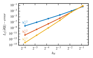
Figure 2: 2.50 confirms the convergence rates predicted by Corollary 2.48: the error $\|{\mathbf{r}}_{\mathbf{x}}^{h_{N}}-{\mathbf{r}}_{\mathbf{x}}\|_{L_{2}(\partial\Omega)}$ decays with the algebraic rate 4.51 (for $\mathsf{k}_{4}^{1.2}$), 6.79 (for $\mathsf{k}_{6}^{1.2}$), and 8.77 (for $\mathsf{k}_{8}^{1.2}$).

Remark 2.51.

It is known from scattered data approximation theory [26] that the condition number of $(\mathsf{k}({\mathbf{x}}_{i},{\mathbf{x}}_{j}))_{i,j=1}^{n}$ can be very large for certain collections of points $\{{\mathbf{x}}_{i}\}_{i=1}^{n}$. We have computed the condition number of the saddle point matrix from Eq. 51 for different $\sigma$s and $h_{N}$ and have observed that ,similarly to the condition number of $(\mathsf{k}({\mathbf{x}}_{i},{\mathbf{x}}_{j}))_{i,j=1}^{n}$, it behaves roughly as $(\sigma/h_{N})^{p}$, where $p$ is the polynomial order of the Wendland’s kernel. Note that by combining Gershgorin’s theorem [34, Ch. 12, see p. 207] and the result listed in [34, Ch. 12.2, Table 12.1], it is possible to show that the condition number of $(\mathsf{k}({\mathbf{x}}_{i},{\mathbf{x}}_{j}))_{i,j=1}^{n}$ is bounded from above by $C(h_{N})^{-p}$, where $C$ is a positive constant.

3 Application to shape Newton methods

The formulation of shape Newton methods is a delicate task, and not all second-order shape derivatives are suited for this job. The study of second-order shape derivatives is out of the scope of this work, and we refer an interested reader to [32, 27]. In this section, we briefly recall the shape Newton method introduced in [32], discuss its discretisation with the weakly-normal functions ${\mathbf{r}}_{\mathbf{x}}$s, and perform some numerical simulations for an unconstrained shape optimisation test case. This test case is kept simple on purpose in order to restrict the discretisation error to the use of weakly-normal basis functions. In this section, we use ${\cal X}={\cal Y}$ in Definition 2.29.

3.1 Shape derivatives and their structure theorem

We begin by recalling the definition of shape derivatives and their structure theorem from [32]. For a given set $\mathsf{D}\subset{\mathbf{R}}^{2}$, we denote by $\wp(\mathsf{D})$ the powerset of $\mathsf{D}$. Furthermore we use the notation $\accentset{\circ}{C}^{1}(\mkern 1.5mu\overline{\mkern-1.5mu\mathsf{D}\mkern-1.5mu}\mkern 1.5mu,{\mathbf{R}}^{d})$ to indicate the Banach space of functions ${\mathbf{X}}\in C^{1}(\mkern 1.5mu\overline{\mkern-1.5mu\mathsf{D}\mkern-1.5mu}\mkern 1.5mu,{\mathbf{R}}^{d})$ that satisfy ${\mathbf{X}}=0$ on $\partial\mathsf{D}$.

Definition 3.1.

Let $J:\Xi\subset\wp(\mathsf{D})\rightarrow{\mathbf{R}}$ be a shape function, and let ${\mathbf{X}},{\mathbf{Y}}\in\accentset{\circ}{C}^{1}(\mkern 1.5mu\overline{\mkern-1.5mu\mathsf{D}\mkern-1.5mu}\mkern 1.5mu,{\mathbf{R}}^{2})$ be two vector fields.
(i) The directional derivative of $J$ at $\Omega\in\Xi$ in the direction ${\mathbf{X}}$ is defined by

(72) $$DJ(\Omega)({\mathbf{X}})\coloneqq\lim_{t\to 0^{+}}\frac{J((\operatorname{\mathbf{id}}+t{\mathbf{X}})(\Omega))-J(\Omega)}{t}.$$

(ii) The second directional derivative of $J$ at $\Omega$ in the direction $({\mathbf{X}},{\mathbf{Y}})$ is defined by

(73) $$\mathfrak{D}^{2}J(\Omega)({\mathbf{X}})({\mathbf{Y}})=\lim_{t\to 0^{+}}\frac{DJ((\operatorname{\mathbf{id}}+t{\mathbf{Y}})(\Omega))({\mathbf{X}}\circ(\operatorname{\mathbf{id}}+t{\mathbf{Y}})^{-1})-DJ(\Omega)({\mathbf{X}})}{t},$$

(assuming that $DJ((\operatorname{\mathbf{id}}+t{\mathbf{Y}})(\Omega))({\mathbf{X}}\circ(\operatorname{\mathbf{id}}+t{\mathbf{Y}})^{-1})$ exists for all small $t$).

Remark 3.2.

Assume that the map $J_{\Omega}:\accentset{\circ}{C}^{1}(\mkern 1.5mu\overline{\mkern-1.5mu\mathsf{D}\mkern-1.5mu}\mkern 1.5mu,{\mathbf{R}}^{d})\to{\mathbf{R}}$, ${\mathbf{X}}\mapsto J((\operatorname{\mathbf{id}}+{\mathbf{X}})(\Omega))$ is twice Fréchet differentiable at $0$. Then, the bilinear operator $({\mathbf{X}},{\mathbf{Y}})\mapsto\mathfrak{D}^{2}J(\Omega)({\mathbf{X}})({\mathbf{Y}})$ is the second derivative of $J_{\Omega}$ at $0$, and thus symmetric [3, Thm 5.2, pp. 189].

We denote by $\nabla^{\boldsymbol{\tau}}f$ the tangential gradient of function $f$ and by ${\mathbf{X}}_{\boldsymbol{\tau}}\coloneqq{\mathbf{X}}|_{\partial\Omega}-({\mathbf{X}}|_{\partial\Omega}\cdot\boldsymbol{\nu})\boldsymbol{\nu}$ the tangential component of a vector field ${\mathbf{X}}$ on $\partial\Omega$. The shape derivatives $DJ$ and $\mathfrak{D}^{2}J$ are characterised by the following structure theorem (see [32, 23]).

Theorem 3.3.

Assume that $J$ is twice differentiable at $\Omega$ and assume that $\Omega$ is of class $C^{3}$. Then, there are continuous functionals $\mathfrak{g}:C^{1}(\partial\Omega)\to{\mathbf{R}}$ and $\mathfrak{h}:C^{1}(\partial\Omega)\times C^{1}(\partial\Omega)\to{\mathbf{R}}$, such that

(74) $$DJ(\Omega)({\mathbf{X}})=\mathfrak{g}({\mathbf{X}}|_{\partial\Omega}\cdot\boldsymbol{\nu})\qquad\qquad\text{for all }{\mathbf{X}}\in\accentset{\circ}{C}^{1}(\mkern 1.5mu\overline{\mkern-1.5mu\mathsf{D}\mkern-1.5mu}\mkern 1.5mu,{\mathbf{R}}^{2})\,,$$

and

(75) $$\begin{split}\mathfrak{D}^{2}J(\Omega)({\mathbf{X}})({\mathbf{Y}})=&\mathfrak{h}({\mathbf{X}}_{|_{\partial\Omega}}\cdot\boldsymbol{\nu},{\mathbf{Y}}_{|_{\partial\Omega}}\cdot\boldsymbol{\nu})-\mathfrak{g}(\boldsymbol{\nu}\cdot\partial^{\boldsymbol{\tau}}{\mathbf{X}}_{\boldsymbol{\tau}}{\mathbf{Y}}_{\boldsymbol{\tau}})\\ &-\mathfrak{g}(\nabla^{\boldsymbol{\tau}}({\mathbf{Y}}\cdot\boldsymbol{\nu})\cdot{\mathbf{X}}_{\boldsymbol{\tau}})-\mathfrak{g}(\nabla^{\boldsymbol{\tau}}({\mathbf{X}}\cdot\boldsymbol{\nu})\cdot{\mathbf{Y}}_{\boldsymbol{\tau}})\end{split}$$

for all ${\mathbf{X}},{\mathbf{Y}}\in\accentset{\circ}{C}^{2}(\mkern 1.5mu\overline{\mkern-1.5mu\mathsf{D}\mkern-1.5mu}\mkern 1.5mu,{\mathbf{R}}^{2})$.

Remark 3.4.

The function $\mathfrak{h}$ corresponds to a Banach space version of the Riemannian Hessian on shape spaces used in [28, Def. 2.2, p. 488].

Remark 3.5.

Notice that Eq. 75 is equivalent to (see [23])

(76) $$\mathfrak{D}^{2}J(\Omega)({\mathbf{X}})({\mathbf{Y}})=\mathfrak{h}({\mathbf{X}}_{|_{\partial\Omega}}\cdot\boldsymbol{\nu},{\mathbf{Y}}_{|_{\partial\Omega}}\cdot\boldsymbol{\nu})-\mathfrak{g}(\boldsymbol{\nu}\cdot\partial^{\boldsymbol{\tau}}{\mathbf{Y}}{\mathbf{X}}_{\boldsymbol{\tau}})-\mathfrak{g}({\mathbf{Y}}_{\boldsymbol{\tau}}\cdot\partial^{\boldsymbol{\tau}}\boldsymbol{\nu}{\mathbf{X}}_{\boldsymbol{\tau}})-\mathfrak{g}(\boldsymbol{\nu}\cdot\partial^{\boldsymbol{\tau}}{\mathbf{X}}{\mathbf{Y}}_{\boldsymbol{\tau}}).$$

3.2 Shape Newton descent directions and their approximation

In this section, we define the shape Newton equation and its approximation with weakly-normal basis functions. For a particular test case, we derive quasi-optimality of the approximate Newton update and verify the resulting convergence rates with a numerical experiment. Henceforth, $\Omega\subset{\mathbf{R}}^{2}$ is a set with $C^{k+1}$-boundary (with $k\geq 1$), and $\mathcal{H}({\mathbf{R}}^{2})$ is a RKHS that satisfies 2.8.

Definition 3.6.

The ${\cal H}({\mathbf{R}}^{2})$-Newton descent direction at $\Omega$ is the solution ${\mathbf{X}}_{\boldsymbol{\nu}}\in[\mathcal{H}(\partial\Omega)]_{\boldsymbol{\nu}}$ of

(77) $$\mathfrak{D}^{2}J(\Omega)({\mathbf{X}}_{\boldsymbol{\nu}})({\mathbf{Y}})=-DJ(\Omega)({\mathbf{Y}})\quad\text{ for all }{\mathbf{Y}}\in[{\cal H}(\partial\Omega)]^{2}_{\boldsymbol{\nu}}.$$

Remark 3.7.

If $J$ satisfies the assumptions of Theorem 3.3 and the functions in $\mathcal{H}(\partial\Omega)$ are sufficiently smooth (for instance, $\mathcal{H}(\partial\Omega)\subset C^{2}(\partial\Omega)$), then formulas (74) and (75) satisfy

$$\mathfrak{D}^{2}J(\Omega)({\mathbf{r}}_{\mathbf{x}})({\mathbf{r}}_{\mathbf{y}})=\mathfrak{h}({\mathbf{r}}_{\mathbf{x}}\cdot\boldsymbol{\nu},{\mathbf{r}}_{\mathbf{y}}\cdot\boldsymbol{\nu})\quad\text{and}\quad DJ(\Omega)({\mathbf{r}}_{\mathbf{y}})=\mathfrak{g}({\mathbf{r}}_{\mathbf{y}}\cdot\boldsymbol{\nu})\quad\text{for all }{\mathbf{x}},{\mathbf{y}}\in\partial\Omega,$$

because item (a) from Theorem 2.18 implies $({\mathbf{r}}_{\mathbf{x}})_{\boldsymbol{\tau}}=({\mathbf{r}}_{\mathbf{y}})_{\boldsymbol{\tau}}=0$. This, in light of Theorem 2.27, implies that Eq. 77 is equivalent to

(78) $$\mathfrak{h}({\mathbf{X}}_{\boldsymbol{\nu}}\cdot\boldsymbol{\nu},{\mathbf{r}}_{\mathbf{y}}\cdot\boldsymbol{\nu})=-\mathfrak{g}({\mathbf{r}}_{\mathbf{y}}\cdot\boldsymbol{\nu})\quad\text{ for all }\quad{\mathbf{y}}\in\partial\Omega.$$

Since $\mathfrak{h}$ and $\mathfrak{g}$ are (bi)linear and continuous in $C^{1}({\mathbf{R}}^{2})$, equation Eq. 78 can also be used to define ${\cal H}({\mathbf{R}}^{2})$-Newton descent direction for RKHS that satisfy only ${\cal H}({\mathbf{R}}^{2})\subset C^{1}({\mathbf{R}}^{2})$. For instance, as mentioned in Example 2.5, the native space of the kernel $\mathsf{k}_{2}^{\sigma}$ is ${\cal H}({\mathbf{R}}^{2})=H^{2.5}({\mathbf{R}}^{2})$, and $H^{2.5}({\mathbf{R}}^{2})\subset C^{1,1/2}({\mathbf{R}}^{2})$ by the Sobolev embedding theorem (where $C^{1,1/2}({\mathbf{R}}^{2})$ denotes the usual Hölder space).

In general, it can be difficult to compute an exact solution of Eq. 77 because $\mathfrak{D}^{2}J$ and $DJ$ are typically given by very complicated formulas. For instance, when $J$ is constrained by a PDE, the formula of $\mathfrak{D}^{2}J$ contains the material derivative of the solution of the PDE-constraint [8]. Nevertheless, approximate ${\cal H}({\mathbf{R}}^{2})$-Newton descent directions can be computed by discretising Eq. 77 with the weakly-normal basis functions ${\mathbf{r}}_{\mathbf{x}}$s.

Definition 3.8.

Let $\mathcal{X}_{N}=\{{\mathbf{x}}_{1},\ldots,{\mathbf{x}}_{N}\}\subset\partial\Omega$ be a collection of pairwise distinct points, and let $h=h_{\mathcal{X}_{N},\partial\Omega}$ denote its fill distance. The approximate ${\cal H}({\mathbf{R}}^{2})$-Newton descent direction at $\Omega$ with respect to ${\cal H}(\partial\Omega)$ is the solution ${\mathbf{X}}_{\boldsymbol{\nu}}^{h}\in{\cal R}_{N}\coloneqq\mathrm{span}\{{\mathbf{r}}_{{\mathbf{x}}}:{\mathbf{x}}\in{\cal X}_{N}\}$ of

(79) $$\mathfrak{D}^{2}J(\Omega)({\mathbf{X}}_{\boldsymbol{\nu}}^{h})({{\mathbf{Y}}^{h}})=-DJ(\Omega)({{\mathbf{Y}}^{h}})\quad\text{ for all }{{\mathbf{Y}}^{h}}\in{\cal R}_{N}.$$

Example 3.9.

We consider the shape function $J(\Omega)=\int_{\Omega}f\;dx$ with $f\in C^{2}({\mathbf{R}}^{2})$. This shape function $J$ can be used as a regularisation in image segmentation; see [19]. Its shape derivatives read [32]

(80) $$DJ(\Omega)({\mathbf{X}})= \int_{\partial\Omega}f{\mathbf{X}}\cdot\boldsymbol{\nu}\;ds\,,$$

(81) $$\mathfrak{D}^{2}J(\Omega)({\mathbf{X}})({\mathbf{Y}})= \int_{\partial\Omega}(\nabla f\cdot\boldsymbol{\nu}+\kappa f)({\mathbf{X}}\cdot\boldsymbol{\nu})({\mathbf{Y}}\cdot\boldsymbol{\nu})\;ds-\int_{\partial\Omega}f\boldsymbol{\nu}\cdot\partial^{\boldsymbol{\tau}}{\mathbf{X}}_{\boldsymbol{\tau}}{\mathbf{Y}}_{\boldsymbol{\tau}}\;ds$$

$$-\int_{\partial\Omega}f\nabla^{\boldsymbol{\tau}}({\mathbf{Y}}\cdot\boldsymbol{\nu})\cdot{\mathbf{X}}+f\nabla^{\boldsymbol{\tau}}({\mathbf{X}}\cdot\boldsymbol{\nu})\cdot{\mathbf{Y}}\;ds,$$

where $\kappa$ denotes the curvature of $\partial\Omega$. Hence the ${\cal H}({\mathbf{R}}^{2})$-Newton descent direction at $\Omega$ is the solution ${\mathbf{X}}_{\boldsymbol{\nu}}\in[\mathcal{H}(\partial\Omega)]_{\boldsymbol{\nu}}$ of

(82) $$\int_{\partial\Omega}(\nabla f\cdot\boldsymbol{\nu}+\kappa f)({{\mathbf{X}}}_{\boldsymbol{\nu}}\cdot\boldsymbol{\nu})({{\mathbf{Y}}}\cdot\boldsymbol{\nu})\;ds=-\int_{\partial\Omega}f({{\mathbf{Y}}}\cdot\boldsymbol{\nu})\;ds\quad\text{ for all }{{\mathbf{Y}}}\in[\mathcal{H}(\partial\Omega)]_{\boldsymbol{\nu}}.$$

Note that, when it exists, the solution of Eq. 82 is ${\mathbf{X}}_{\boldsymbol{\nu}}=(-f/(\nabla f\cdot\boldsymbol{\nu}+\kappa f))\boldsymbol{\nu}$. Clearly, it is possible to approximate ${\mathbf{X}}_{\boldsymbol{\nu}}$ by interpolating it on ${\cal R}_{N}$. However, note that this interpolant would not satisfy Eq. 79. Finally, we point out that Eq. 80 implies that zero-level sets of $f$ are local optima for this shape optimization problems. This implies that, close to the optimum, the term $\kappa f$ in Eq. 82 plays a minor role compared to $\nabla f\cdot\boldsymbol{\nu}$. For this reasons, some authors omit the term $\kappa f$ in the computation of Newton updates [32, 28].

Proposition 3.10 shows quasi-optimality of the approximate shape Newton updates when the shape derivatives are as in Example 3.9.

Proposition 3.10.

Let $J(\Omega)=\int_{\Omega}f\;dx$ with $f\in C^{2}({\mathbf{R}}^{2})$, and further assume that $\nabla f\cdot\boldsymbol{\nu}+\kappa f>0$ on $\partial\Omega$. Then, the solution ${\mathbf{X}}_{\boldsymbol{\nu}}^{h}\in{\cal R}_{N}$ of Eq. 79 satisfies

(83) $$\|{\mathbf{X}}_{\boldsymbol{\nu}}-{\mathbf{X}}_{\boldsymbol{\nu}}^{h}\|_{L_{2}(\partial\Omega)}\leq c_{f,\Omega}\inf_{{\mathbf{Y}}\in{\cal R}_{N}}\|{\mathbf{X}}_{\boldsymbol{\nu}}-{\mathbf{Y}}\|_{L_{2}(\partial\Omega)}\,.$$

Proof 3.11.

The bilinear form

(84) $$L_{2}(\partial\Omega)\times L_{2}(\partial\Omega)\to\mathbb{R}\,,\quad(x,y)\mapsto\int_{\partial\Omega}(\nabla f\cdot\boldsymbol{\nu}+\kappa f)xy\;ds$$

is $L_{2}(\partial\Omega)$-continuous, symmetric, and $L_{2}(\partial\Omega)$-elliptic. Let ${\cal Z}_{N}\coloneqq\mathrm{span}\{{\mathbf{X}}\cdot\boldsymbol{\nu}:{\mathbf{X}}\in{\cal R}_{N}\}$. Clearly, ${\cal Z}_{N}\subset L_{2}(\partial\Omega)$. Therefore, the solution $z_{h}\in{\cal Z}_{N}$ of

(85) $$\int_{\partial\Omega}(\nabla f\cdot\boldsymbol{\nu}+\kappa f)z_{h}y\;ds=-\int_{\partial\Omega}fy\;ds\quad\text{ for all }y\in{\cal Z}_{N}$$

satisfies

(86) $$\|z-z_{h}\|_{L_{2}(\partial\Omega)}\leq c_{f,\Omega}\inf_{y\in{\cal Z}_{N}}\|z-y\|_{L_{2}(\partial\Omega)}\,,$$

where $z\in L_{2}(\partial\Omega)$ is the solution of

(87) $$\int_{\partial\Omega}(\nabla f\cdot\boldsymbol{\nu}+\kappa f)zy\;ds=-\int_{\partial\Omega}fy\;ds\quad\text{ for all }y\in L_{2}(\partial\Omega)\,.$$

Finally, ${\mathbf{X}}_{\boldsymbol{\nu}}^{h}=z_{h}\boldsymbol{\nu}$, because ${\cal R}_{N}$ satisfies ${\cal R}_{N}=\{z\boldsymbol{\nu}:z\in{\cal Z}_{N}\}$, and ${\mathbf{X}}_{\boldsymbol{\nu}}=z\boldsymbol{\nu}$, because the solution of Eq. 87 is $z=-f/(\nabla f\cdot\boldsymbol{\nu}+\kappa f)$.

Numerical Experiment 3.12.

We perform a numerical experiment to investigate the approximation error Eq. 83 for $f({\mathbf{x}})=|{\mathbf{x}}|^{2}-1$. We choose $\partial\Omega$ to be the ellipse depicted in Fig. 1 (left) and consider the sequence of subsets

(88) $${\cal X}_{N}=\{\gamma(2\pi\ell/N):\ell=1,\dots,N\}\quad\text{with}\quad N=2^{4},2^{5},\dots,2^{8}\,.$$

For each $N$, we construct the finite dimensional space $\widetilde{\cal R}_{N}\coloneqq\mathrm{span}\{{\mathbf{r}}^{h_{N}}_{{\mathbf{x}}}:{\mathbf{x}}\in{\cal X}_{N}\}$ (where $h_{N}$ denotes the fill distance of ${\cal X}_{N}$), and compute the solution $\widetilde{\mathbf{X}}_{\boldsymbol{\nu}}^{h_{N}}\in\widetilde{\cal R}_{N}$ of

(89) $$\int_{\partial\Omega}(\nabla f\cdot\boldsymbol{\nu}+\kappa f)(\widetilde{\mathbf{X}}_{\boldsymbol{\nu}}^{h_{N}}\cdot\boldsymbol{\nu})({{\mathbf{Y}}^{h_{N}}}\cdot\boldsymbol{\nu})\;ds=-\int_{\partial\Omega}f({{\mathbf{Y}}^{h_{N}}}\cdot\boldsymbol{\nu})\;ds\quad\text{ for all }{{\mathbf{Y}}^{h_{N}}}\in\widetilde{\cal R}_{N}.$$

Although the normal vector field $\boldsymbol{\nu}$ and curvature $\kappa$ can be computed exactly, for the ease of implementation we replace the curve $\gamma$ with a highly accurate interpolant (using Chebfun [10]) and evaluate $\boldsymbol{\nu}$ and $\kappa$ of this interpolant. For a result on this kind of approximation, see [33]. Finally, we compute (with sufficiently many quadrature points) the $L_{2}(\partial\Omega)$-absolute error $\|{\mathbf{X}}_{\boldsymbol{\nu}}-\widetilde{\mathbf{X}}_{\boldsymbol{\nu}}^{h_{N}}\|_{L_{2}(\partial\Omega)}$. In Fig. 3, we plot this $L_{2}$-errors versus $h_{N}$ (measured with the Euclidean distance) for the kernels $\mathsf{k}_{4}^{0.7}$, $\mathsf{k}_{6}^{0.7}$, and $\mathsf{k}_{8}^{0.7}$. The measured convergence rates read (approximatively) 4.20, 5.98, and 8.20 (when $h_{N}>2^{-4}$), respectively. Similar compatible results are obtained for the nonconvex domain depicted in Fig. 1 (left), as well as for different values of $\sigma$. To intepret these results, let us first point out that $\widetilde{\cal R}_{N}$ is only an approximation of ${\cal R}_{N}$. It may not be so simple to prove a proposition for $\widetilde{\cal R}_{N}$ that is analogous to Proposition 3.10, because $\widetilde{\cal R}_{N}$ does not contain the image of the operator ${\mathbf{X}}\mapsto({\mathbf{X}}\cdot\boldsymbol{\nu})\boldsymbol{\nu}$. Note also that it is true that ${\mathbf{r}}_{\mathbf{x}}^{h_{N}}$ converges to ${\mathbf{r}}_{\mathbf{x}}$ as $h_{N}\to 0$, but Theorem 2.46 does not guarantee that this convergence is uniform in ${\mathbf{x}}$. However, if we assume that a proposition analogous to Proposition 3.10 exists for $\widetilde{\cal R}_{N}$, we can explain the measured convergence rates with [17, Cor. 15], because interpolating a vector field ${\mathbf{f}}$ into $\widetilde{\cal R}_{N}$ or into ${\cal H}({\cal X}_{N})\times{\cal H}({\cal X}_{N})$ returns exactly the same interpolant if the vector field ${\mathbf{f}}$ is normal to $\partial\Omega$.

Finally, the convergence history saturates for $\mathsf{k}_{8}^{0.7}$ because the condition number of the discretised shape Hessian is very large for $N=2^{8}$ (the Matlab-function cond returns the value 4.826490e+18). In a simple numerical experiment, we observed that the condition number of the discretised shape Hessian behaves as $h_{N}^{\alpha_{h}}\sigma^{\alpha_{\sigma}}$ with $\alpha_{h}=-8.7$ and ${\alpha_{\sigma}}=7.2$ when $p=4$ and $\alpha_{h}=-12.48$ and ${\alpha_{\sigma}}=10.18$ when $p=6$. We believe that these condition numbers deteriorate because we rely on radial basis functions. Indeed, following closely [6, Sect. 5.2], it is possible to bound from above the condition number of a mass matrix the arises from a discretization based on compactly supported Wendland kernels, and this upper bound reads $Ch_{N}^{-2p}$, where $C$ is a positive constant.

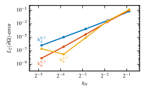
Figure 3: 3.12 shows that $\|{\mathbf{X}}_{\boldsymbol{\nu}}-\widetilde{\mathbf{X}}_{\boldsymbol{\nu}}^{h_{N}}\|_{L_{2}(\partial\Omega)}$ decays with the algebraic rate 4.20 (for $\mathsf{k}_{4}^{0.7}$), 5.98 (for $\mathsf{k}_{6}^{0.7}$), and 8.20 (for $\mathsf{k}_{8}^{0.7}$ when $h_{N}>2^{-4}$).

3.3 Discrete shape Newton algorithm based on ${\mathbf{r}}_{\mathbf{x}}$

In this section, we use the basis functions ${\mathbf{r}}_{\mathbf{x}}$s to formulate a discrete shape Newton algorithm and test it on Example 3.9. In particular, we investigate the impact of the Newton update approximation on the convergence rates of the shape Newton method. To measure these convergence rates, we use the norm on the tangent spaces, which is simply the norm of the RKHS.

Let $J$ be a twice differentiable shape function, $\Omega\subset{\mathbf{R}}^{2}$ be an initial guess, and ${\cal X}_{N}=\{{\mathbf{x}}_{1},\ldots,{\mathbf{x}}_{N}\}$ be a finite number points on $\partial\Omega$. We begin by specifying how to transport the basis functions ${\mathbf{r}}_{\mathbf{x}}$ when $\Omega$ is perturbed by a geometric transformation.

Definition 3.13.

Let ${\mathbf{r}}_{\partial\Omega,{\mathbf{x}}}$ denote the weakly-normal function associated with $\partial\Omega$ and ${\mathbf{x}}\in\partial\Omega$, and let $F_{t}:{\mathbf{R}}^{2}\to{\mathbf{R}}^{2}$ be family of $C^{1}$-diffeomorphisms such that $F_{0}=\operatorname{\mathbf{id}}$. We define the transport $\mathfrak{T}_{s}$ by

(90) $$\mathfrak{T}_{s}({\mathbf{r}}_{\partial\Omega,{\mathbf{x}}})\coloneqq{\mathbf{r}}_{F_{s}(\partial\Omega),F_{s}({\mathbf{x}})},$$

and extend it by linearity to $\mathfrak{\mathfrak{T}}_{s}:\mathrm{span}\{{\mathbf{r}}_{\partial\Omega,{\mathbf{x}}},\;{\mathbf{x}}\in\partial\Omega\}\to\mathrm{span}\{\mathfrak{T}_{s}({\mathbf{r}}_{\partial\Omega,{\mathbf{x}}}),\;{\mathbf{x}}\in\partial\Omega\}$. By construction, $\mathfrak{T}_{s}:\mathrm{span}\{{\mathbf{r}}_{\partial\Omega,{\mathbf{x}}},\;{\mathbf{x}}\in\partial\Omega\}\subset[{\cal H}(\partial\Omega)]_{\boldsymbol{\nu}}^{2}\to[{\cal H}(F_{t}(\partial\Omega))]_{\boldsymbol{\nu}}^{2}$.

Using this transport, we formulate the following discrete shape Newton method. Set $\Omega_{0}=\Omega$, and $\widetilde{\cal R}_{N}^{0}\coloneqq\mathrm{span}\{{\mathbf{r}}^{h}_{\partial\Omega,{\mathbf{x}}}:{\mathbf{x}}\in{\cal X}_{N}\}$. The optimisation algorithm proceeds as follows: first, it computes the solution ${\mathbf{g}}_{0}\in\widetilde{\cal R}_{N}^{0}$ of

(91) $$\mathfrak{D}^{2}J(\Omega_{0})({\mathbf{g}}_{0})(\boldsymbol{\varphi})=-DJ(\Omega_{0})(\boldsymbol{\varphi})\quad\text{ for all }\boldsymbol{\varphi}\in\widetilde{\cal R}_{N}^{0};$$

then, it defines the transformation $F_{0}({\mathbf{x}})\coloneqq{\mathbf{x}}+{\mathbf{g}}_{0}({\mathbf{x}})$ and the new domain $\Omega_{1}\coloneqq F_{0}(\Omega_{0})$; finally, it defines the space $\widetilde{\cal R}_{N}^{1}$ by transporting $\widetilde{\cal R}_{N}^{0}$ with $F_{0}$, that is,

(92) $$\widetilde{\cal R}_{N}^{1}\coloneqq\mathrm{span}\{{\mathbf{r}}^{h}_{F_{0}(\partial\Omega),F_{0}({\mathbf{x}})}:{\mathbf{x}}\in{\cal X}_{N}\}\,.$$

This procedure is repeated until convergence.

Remark 3.14.

The shape $\Omega_{1}$ that results by updating $\Omega_{0}$ with ${\mathbf{g}}_{0}$ has the same regularity of ${\mathbf{g}}_{0}$. Therefore, from a theoretical point of view, it may be necessary to regularise the update ${\mathbf{g}}_{0}$ to guarantee that 2.8 remains fulfilled during the optimisation process. However, such a regularization is not necessary in practice when one employs the Wendland kernels from Example 2.5. In this case, regularity is lost only at the points $\{{\mathbf{x}}\pm\sigma:{\mathbf{x}}\in{\cal X}_{N}\}$, whereas to construct the approximate weakly-normal function ${\mathbf{r}}_{\mathbf{x}}^{h}$s it is necessary to evaluate $\boldsymbol{\nu}$ and $\boldsymbol{\tau}$ only at ${\cal X}_{N}$. Therefore, if $\{{\mathbf{x}}\pm\sigma:{\mathbf{x}}\in{\cal X}_{N}\}\cap{\cal X}_{N}=\emptyset$, the discrete algorithm does not perceive the loss of regularity of the domain.

Numerical Experiment 3.15.

We test this discrete shape Newton method by performing 5 optimisation steps to solve Example 3.9 with $f({\mathbf{x}})=|{\mathbf{x}}|^{2}-1$ and

(93) $$\Omega=\{\gamma(\phi)=(0.2+1.15\cos(\phi),0.15+0.9\sin(\phi)):\phi\in[0,2\pi)\}\,.$$

The (approximate) weakly-normal basis functions ${\mathbf{r}}^{h}_{\mathbf{x}}$ are constructed with the kernel $\mathsf{k}_{4}^{0.7}$ on the sets

(94) $${\cal X}_{N}=\{\gamma(2\pi\ell/N):\ell=1,\dots,N\}\quad\text{with}\quad N=2^{4},2^{5},\dots,2^{8}\,.$$

To simplify the implementation, the shape iterates $\{\Omega_{\ell+1}=\Omega_{\ell}+{\mathbf{g}}_{\ell}(\Omega_{\ell})\}_{\ell=0}^{4}$ are replaced by highly-accurate interpolants computed with Chebfun [10]. Normal and tangential vector fields $\boldsymbol{\nu}$ and $\boldsymbol{\tau}$, as well as the curvature term $\kappa$, are approximated evaluating their corresponding analytic formulas with these interpolants.

To replicate the results from [32, 28], we approximate Newton descent direction neglecting the curvature term in Eq. 82. Note that a counterpart of Proposition 3.10 can be proved, provided that $\nabla f\cdot\boldsymbol{\nu}>0$ (which is the case in these experiments). In Fig. 4, we plot the evolution of the shape iterates $\{\Omega_{\ell}\}_{\ell=0}^{2}$ for $N=2^{4}$ (top left) and for $N=2^{5}$ (top right), and, for each $N$, we plot the values of the sequence $\{\|{\mathbf{g}}_{\ell}\|_{[{\cal H}]^{2}}\}_{\ell=0}^{4}$ (bottom left) and the measure of the quadratic rate of convergence $\{\|{\mathbf{g}}_{\ell+1}\|_{[{\cal H}]^{2}}/\|{\mathbf{g}}_{\ell}\|_{[{\cal H}]^{2}}^{2}\}_{\ell=0}^{3}$ (bottom right).

We observe that the sequence of shapes converges quickly to the minimiser (a circle of radius 1 centered in the origin), and that the discretisation error on the retrieved shape is not visible for $N\geq 2^{5}$. We also observe that the discretised shape Newton method converges quadratically, if sufficiently many weakly-normal vector fields are employed.

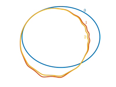
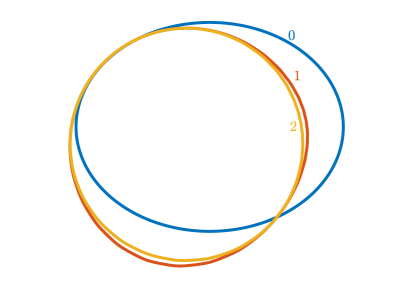
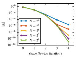
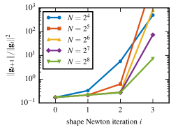
Figure 4: 3.15 shows that the discretised shape Newton method converges quadratically, if sufficiently many weakly-normal vector fields are employed.

Remark 3.16.

We have repeated the previous experiment including the curvature term in the Newton equation. Surprisingly, we observed that the quadratic rate of convergence deteriorates to superlinear although the sequence of shape iterates converge to the correct minimiser. To further investigate this unexpected behavior, we consider a simpler scenario that can be solved analytically. Let the initial domain $\Omega_{0}$ be a disc of radius $r_{0}$ centered in the origin. In this case, the shape iterates are concentric discs of radii

(95) $$r_{\ell+1}=r_{\ell}-\frac{r_{\ell}^{2}-1}{2r_{\ell}+\kappa_{\ell}(r_{\ell}^{2}-1)}\,,\quad\ell=0,1,\ldots,$$

where $\kappa_{\ell}=r_{\ell}^{-1}$ is the curvature of the $\ell$th disc. Equation (95) can be rewritten as

(96) $$r_{\ell+1}=\frac{2r_{\ell}^{3}}{3r_{\ell}^{2}-1}\,.$$

From this equation, we see that if $r_{\ell}<1/\sqrt{3}$, then $r_{\ell+1}<0$, which is not feasible. On the other hand, if $r_{\ell}>1/\sqrt{3}$, then $r_{\ell+1}>1$. Moreover, $r_{\ell+1}<r_{\ell}$ if $r_{\ell}>1$, which implies that $(r_{\ell})$ decreases monotonically and converges to one. By direct computation, we can show that

(97) $$|1-r_{\ell+1}|=\left|\frac{(2r_{\ell}+1)(r_{\ell}-1)}{3r_{\ell}^{2}-1}\right||1-r_{\ell}|\,,$$

which implies that the error is decreasing only if $r_{\ell}>{\textstyle\frac{1+\sqrt{41}}{10}}>{\textstyle\frac{1+\sqrt{36}}{10}}=0.7$. Since $r_{\ell}>1/\sqrt{3}$ implies $r_{\ell+1}>1$, the sequence $\{r_{\ell}\}$ converges quadratically for every initial radius $r_{0}>1/\sqrt{3}$ after the first iteration. However, we obtain a better algorithm if we set $\kappa_{\ell}=0$, because equation (95) becomes

$$r_{\ell+1}=\frac{1}{2}\left(r_{\ell}+\frac{1}{r_{\ell}}\right)\,,$$

which converges quadratically for any $r_{0}>0$. To be more precise, in this case

(98) $$|r_{\ell+1}-1|=\left|\frac{r_{\ell}-1}{2r_{\ell}}\right||r_{\ell}-1|,$$

which converges faster than (97) because ${\textstyle\frac{2r_{\ell}+1}{3r_{\ell}^{2}-1}}>{\textstyle\frac{1}{2r_{\ell}}}$ for $r_{\ell}>{\textstyle\frac{1}{\sqrt{3}}}$.This example shows that the denominator in (95) plays a key role in the convergence analysis, and it may be for the same reason that the shape Newton algorithm without curvature term performed better in our previous numerical experiment.

Numerical Experiment 3.17.

To further highlight the effect of the discretisation parameter $N$ on approximate shape Newton methods, we consider the shape optimization problem from Example 3.9 with $f({\mathbf{x}})=f(x,y)=(x^{2}+16y^{2}-1)(x^{2}+(y-0.45)^{2}-0.04)$. The zero-level set of this function is the union of a disc and an ellipse, and it has a cusp at (0, 0.25) (see Fig. 5). Therefore, the optimal shape is not even Lipschitz, and retrieving it by solving the optimization problem is particularly challenging.

We perform 15 discrete shape Newton steps with the same numerical setup of 3.15 In Fig. 5, we plot the evolution of shape iterates $\{\Omega_{\ell}\}_{\ell=0}^{15}$ for $N=2^{6}$ (left) and for $N=2^{8}$ (right). These plots clearly show that increasing $N$ allows retrieving a much better approximation of the optimal shape. Note that, after 15 steps, the algorithm has fully converged to an approximate optimum.

Note that these shape iterates have been computed neglecting the curvature term in Eq. 82. Similarly to 3.15, we have observed that the performance of shape Newton’s method deteriorates if the curvature term is taken into account. In particular, it is necessary both to regularized Newton’s equation to enforce coercivity [20] and to switch to damped Newton’s method to ensure that every shape iterate is feasible.

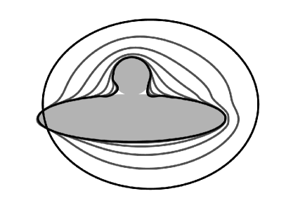
Figure 5: 3.17 shows that increasing the discretisation parameter $N$ allows retrieving a much better approximation of the optimal shape. In these plots, the black lines denote the initial and the final shape, whereas lighter lines denote intermediate shape iterates and the gray area denotes the zero-level set of $f$.

4 Conclusion

In the first part of this work, we have introduced the class of weakly-normal vector fields, which are defined as solutions of saddle point variational problems in RKHSs. Besides investigating their properties, we have discussed their approximation and proved the related convergence rates. These vector fields can be used to discretise shape Newton methods because they have purely normal components.

In the second part of this work, we have formulated a discrete shape Newton method based on these weakly-normal vector fields and, for a specific test case, proved that the discrete shape Newton direction converges to the continuous one in the metric associated with the shape Hessian. Finally, we have showed that the discrete shape Newton method exhibits quadratic convergence if the discretisation error is sufficiently small.

We have observed that our approach leads to the matrices whose condition number deteriorates as the number of degrees of freedom increases. This is a common issue of discretizations based on radial basis functions. In [6], the authors describe a multilevel residual correction algorithm that leads to approximation matrices with bounded condition number. Although there is a debate on its convergence properties [35], this algorithm performed well in numerical experiments, and it would be interesting to investigate whether a similar technique could be used in our context.

The weakly-normal vector fields have another property that has not been exploited in this work: although defined on the boundary $\partial\Omega$, they can be straightforwardly extended to ${\mathbf{R}}^{2}$. This implies that the discrete shape Newton method remains well-posed even when formulated with volume-based expressions of the shape derivative and the shape Hessian. This is a great advantage for PDE-constrained shape optimisation problems, in which case volume based formulas are easier to derive and impose less regularity requirements on the solution of the PDE-constraint. However, using volume-based formulas requires the integration of the weakly-normal vector fields on $\Omega$, which introduces an additional complexity in the implementation as well as additional sources of discretisation error that need to be analysed. For this reason, we postpone to a subsequent work the study of the shape Newton method based on weakly-normal vector fields in the framework of PDE-constrained shape functionals.

Finally, we mention that certain shape optimization problems present an additional difficulty: their second-order shape derivative is continuous on a function space and coercive on a weaker one (this is commonly known as the “norm gap”). When this is the case, the shape optimization problem under consideration is not well posed [15]. Although discretisation is a form of regularization, in the case of an ill-posed problem one should pay additional care to the discretisation level. The weakly-normal vector fields introduced in this work may carry extra regularization properties because their smoothness can be tuned by choosing appropriate reproducing kernels. We defer the investigation of this interesting aspect to future work.

Appendix

In this appendix, we show that $\mathcal{H}(\partial\Omega)\subset C^{0}(\partial\Omega)$ when $\mathsf{k}\in C^{0}({\mathbf{R}}^{2}\times{\mathbf{R}}^{2})$. We believe that this result is not new, but we could not find its proof in the literature.

Lemma 4.1.

Let $\mathsf{k}$ be a symmetric positive-definite kernel on ${\mathbf{R}}^{2}$. Denote by $\mathcal{H}(\partial\Omega)$ the RKHS associated with the restriction of $\mathsf{k}$ to $\partial\Omega$. If $\mathsf{k}\in C^{0}({\mathbf{R}}^{2}\times{\mathbf{R}}^{2})$, then $\mathcal{H}(\partial\Omega)\subset C^{0}(\partial\Omega)$.

Proof 4.2.

For a generic $f\in{\cal H}(\partial\Omega)$, the reproducing kernel properties of $\mathcal{H}(\partial\Omega)$ implies

(99) $$\begin{split}|f({\mathbf{x}})-f({\mathbf{y}})|&=|(\mathsf{k}({\mathbf{x}},\cdot),f)_{\cal H}-(\mathsf{k}({\mathbf{y}},\cdot),f)_{\cal H}|\\ &=|(\mathsf{k}({\mathbf{x}},\cdot)-\mathsf{k}({\mathbf{y}},\cdot),f)_{\cal H}|\\ &\leq\|\mathsf{k}({\mathbf{x}},\cdot)-\mathsf{k}({\mathbf{y}},\cdot)\|_{{\cal H}}\|f\|_{{\cal H}}\end{split}$$

for all ${\mathbf{x}},{\mathbf{y}}\in\partial\Omega$. Moreover,

(100) $$\|\mathsf{k}({\mathbf{x}},\cdot)-\mathsf{k}({\mathbf{y}},\cdot)\|_{{\cal H}}^{2}=\mathsf{k}({\mathbf{x}},{\mathbf{x}})+\mathsf{k}({\mathbf{y}},{\mathbf{y}})-2\mathsf{k}({\mathbf{x}},{\mathbf{y}})\,.$$

Therefore, the right hand side of Eq. 100 goes to zero as ${\mathbf{x}}$ goes to ${\mathbf{y}}$ because $\mathsf{k}\in C^{0}({\mathbf{R}}^{2}\times{\mathbf{R}}^{2})$. In view of estimate Eq. 99 and Eq. 65, this shows that $f$ is continuous on $\partial\Omega$.

References

• [1] G. Allaire, E. Cancès, and J.-L. Vié, Second-order shape derivatives along normal trajectories, governed by hamilton-jacobi equations, Structural and Multidisciplinary Optimization, 54 (2016), pp. 1245–1266.
• [2] G. Allaire, C. Dapogny, and P. Frey, Shape optimization with a level set based mesh evolution method, Comput. Methods Appl. Mech. Engrg., 282 (2014), pp. 22–53.
• [3] H. Amann and J. Escher, Analysis II, Birkhäuser Basel, 2006.
• [4] K. Bandara, F. Cirak, G. Of, O. Steinbach, and J. Zapletal, Boundary element based multiresolution shape optimisation in electrostatics, J. Comput. Phys., 297 (2015), pp. 584–598.
• [5] D. Boffi, F. Brezzi, and M. Fortin, Mixed finite element methods and applications, Springer, Heidelberg, 2013.
• [6] A. Chernih and Q. Le Gia, Multiscale methods with compactly supported radial basis functions for galerkin approximation of elliptic PDEs, IMA Journal of Numerical Analysis, 34 (2014), pp. 569–591.
• [7] C. Dapogny, R. Estevez, A. Faure, and G. Michailidis, Shape and topology optimization considering anisotropic features induced by additive manufacturing processes. working paper or preprint, Dec. 2017, https://hal.archives-ouvertes.fr/hal-01660850.
• [8] M. C. Delfour and J.-P. Zolésio, Velocity method and Lagrangian formulation for the computation of the shape Hessian, SIAM J. Control Optim., 29 (1991), pp. 1414–1442.
• [9] M. C. Delfour and J.-P. Zolésio, Shapes and geometries: Metrics, analysis, differential calculus, and optimization, Society for Industrial and Applied Mathematics (SIAM), Philadelphia, PA, second ed., 2011.
• [10] T. A. Driscoll, N. Hale, and L. N. Trefethen, eds., Chebfun Guide, Pafnuty Publications, Oxford, 2014, www.chebfun.org.
• [11] M. Eigel and K. Sturm, Reproducing kernel hilbert spaces and variable metric algorithms in PDE-constrained shape optimization, Optimization Methods and Software, 33 (2017), pp. 268–296, https://doi.org/10.1080/10556788.2017.1314471, "https://doi.org/10.1080%2F10556788.2017.1314471,,http://dx.doi.org/10.1080/10556788.2017.1314471".
• [12] I. Ekeland and R. Témam, Convex analysis and variational problems, Society for Industrial and Applied Mathematics (SIAM), Philadelphia, PA, english ed., 1999.
• [13] K. Eppler, Second derivatives and sufficient optimality conditions for shape functionals, Control Cybernet., 29 (2000), pp. 485–511.
• [14] K. Eppler and H. Harbrecht, A regularized Newton method in electrical impedance tomography using shape Hessian information, Control Cybernet., 34 (2005), pp. 203–225.
• [15] K. Eppler and H. Harbrecht, Shape optimization for free boundary problems—analysis and numerics, in Constrained optimization and optimal control for partial differential equations, vol. 160 of Internat. Ser. Numer. Math., Birkhäuser/Springer Basel AG, Basel, 2012, pp. 277–288.
• [16] K. Eppler, H. Harbrecht, and R. Schneider, On convergence in elliptic shape optimization, SIAM J. Control Optim., 46 (2007), pp. 61–83.
• [17] E. Fuselier and G. B. Wright, Scattered data interpolation on embedded submanifolds with restricted positive definite kernels: Sobolev error estimates, SIAM J. Numer. Anal., 50 (2012), pp. 1753–1776.
• [18] A. Henrot and M. Pierre, Variation et optimisation de formes. Une analyse géométrique, Springer, Berlin, 2005.
• [19] M. Hintermüller and W. Ring, A second order shape optimization approach for image segmentation, SIAM J. Appl. Math., 64 (2003/04), pp. 442–467.
• [20] M. Hintermüller and W. Ring, A second order shape optimization approach for image segmentation, SIAM J. Appl. Math., 64 (2003/04), pp. 442–467.
• [21] M. Keuthen and D. Kraft, Shape optimization of a breakwater, Inverse Probl. Sci. Eng., 24 (2016), pp. 936–956.
• [22] A. Laurain and K. Sturm, Distributed shape derivative via averaged adjoint method and applications, ESAIM: M2AN, 50 (2016), pp. 1241–1267.
• [23] A. Novruzi and M. Pierre, Structure of shape derivatives, Journal of Evolution Equations, 2 (2002), pp. 365–382.
• [24] A. Paganini, S. Sargheini, R. Hiptmair, and C. Hafner, Shape optimization of microlenses, Opt. Express, 23 (2015), pp. 13099–13107.
• [25] C. C. D. Ronco, R. Ponza, and E. Benini, Aerodynamic shape optimization of aircraft components using an advanced multi-objective evolutionary approach, Computer Methods in Applied Mechanics and Engineering, 285 (2015), pp. 255 – 290.
• [26] R. Schaback, Error estimates and condition numbers for radial basis function interpolation, Adv. Comput. Math., 3 (1995), pp. 251–264.
• [27] A. Schiela and J. Ortiz, Second order directional shape derivatives, March 2017, http://nbn-resolving.de/urn/resolver.pl?urn=urn:nbn:de:bvb:703-epub-3251-1.
• [28] V. H. Schulz, A Riemannian view on shape optimization, Found. Comput. Math., 14 (2014), pp. 483–501.
• [29] V. H. Schulz, M. Siebenborn, and K. Welker, PDE constrained shape optimization as optimization on shape manifolds, in Geometric science of information, vol. 9389 of Lecture Notes in Comput. Sci., Springer, Cham, 2015, pp. 499–508.
• [30] V. H. Schulz, M. Siebenborn, and K. Welker, Structured inverse modeling in parabolic diffusion problems, SIAM J. Control Optim., 53 (2015), pp. 3319–3338.
• [31] J. Sokołowski and J.-P. Zolésio, Introduction to shape optimization. Shape sensitivity analysis, Springer, Berlin, 1992.
• [32] K. Sturm, Convergence analysis of newton’s method in shape optimization via approximate normal functions, 2016, https://arxiv.org/abs/1608.02699.
• [33] Y. N. Subbotin, Uniform approximation of curvature for smooth classes of plane curves, Proceedings of the Steklov Institute of Mathematics, 297 (2017), pp. 182–185.
• [34] H. Wendland, Scattered data approximation, Cambridge University Press, Cambridge, 2005.
• [35] H. Wendland, Solving Partial Differential Equations with Multiscale Radial Basis Functions, Springer International Publishing, Cham, 2018, pp. 1191–1213, https://doi.org/10.1007/978-3-319-72456-0_55, https://doi.org/10.1007/978-3-319-72456-0_55.