Anti-bunching dynamics of plasmonically mediated entanglement generation

Abstract

Dissipative entanglement generation protocols embrace environmental interactions in order to generate long-lived entangled states. In this letter, we report on the anti-bunching dynamics for a pair of actively driven quantum emitters coupled to a shared dissipative plasmonic reservoir. We find that anti-bunching is a universal signature for entangled states generated by dissipative means and examine its use as an entanglement diagnostic. We discuss the experimental validation of plasmonically mediated entanglement generation by Hanbury Brown-Twiss interferometry with picosecond timing resolution determined by an effective two-qubit Rabi frequency, and we analyze the robustness of entanglement generation with respect to perturbations in local detunings, couplings, and driving fields.

I Introduction

Quantum decoherence results from interactions with unknown or uncontrollable environmental degrees of freedom. This process, by which quantum information deteriorates due to environmental interactions, has been coined information leakageNielsen . It follows that quantum information processing systems should be completely isolated from leaky environments. However, such a task has proven to be quite difficult, and as a consequence, a variety of techniques have been developed to combat the effects of decoherenceTerhal_RMP . With the fault tolerant threshold theorem Aharonov_98 providing a route to overcome decoherence, quantum error correction protocols Shor ; Calderbank ; Laflamme_96 ; Steane ; Gottesman_97 ; Kitaev_97 ; Terhal_RMP , dynamical decoupling protocols Lorenza_DD , and decoherence suppressing quantum control techniques Doherty_2000 ; Dong_Review have all seen substantial progress.

Dissipative driven entanglement (DDE) techniques provide a different and complimentary route to quantum state engineering Verstraete_Nat_Phys . In this paradigm, entanglement is stabilizedReiter_NJP and computations are performedKastoryano_PRL_13 by leveraging select dissipative pathways that are naively assumed to impede long term quantum coherence. Early experimental DDE progress has been achieved in trapped ion Lin_Nature , atomic ensemble Muschik_2011 ; Krauter_2001 , and superconducting Liu_2016 qubit platforms.

Concurrently, a new quantum information processing platform based on the quantum theory of plasmons has rapidly matured in recent years Tame_Review ; Ginzburg_Review . The first demonstration of plasmonically mediated entanglement Altewischer_Nature stimulated developments in both discrete Tame_Review and continuous Lawrie_2013 ; Holtferich_2016 plasmonic quantum variables. More recently, squeezed states of light have enabled ultra-trace plasmonic sensing Fan_2015 ; Lawrie_2016 , while plasmonic mode volumes orders of magnitude below the diffraction limit have enabled Purcell factors exceeding $10^{3}$ in the weak coupling limitAkselrod_2014 and vacuum Rabi splitting in the strong coupling limit Chikkaraddy_2016 ; santhosh2016vacuum . These plasmonic analogs to photonic cavity QED provide a framework for the development of nanoscale architectures with ultrafast coupling dynamics capable of operation at ambient temperatures.

Despite substantial theoretical progress Tudela_2010 ; Cano_2011 ; Nori_2011 ; Tudela_2011 ; Lee_2013 ; Hummer_2013 ; Nerkararyan_2015 ; Ren_2015 ; Gangaraj_2015 ; Hou_15 ; Otten_2015 ; Otten_2016 ; Hakami_2016 , dissipative entanglement generation has yet to be observed in plasmonic platforms. This is partially due to the technical difficulty of integrating plasmonic components with standard readout and control technologies. It is therefore tremendously important to develop alternative yet simple entanglement metrics to develop the nascent field of plasmonic quantum information processing. In this article we address this need by demonstrating how the second order temporal correlation function can be used as a signature of entanglement between a pair of qubits coupled to a common plasmonic environment.

We analytically and numerically treat the dynamics of the dual quantum dot - plasmon hybrid system, illustrated in Fig.  1, and analyze the photon anti-bunching as a function of steady state two qubit entanglement. We also argue that an experimental demonstration is possible, despite the fast qubit timescales inherited from the plasmonic reservoir. Importantly, we show that the two-qubit anti-bunching width can be classically tuned by controlling the external driving fields. Specifically, reducing local driving amplitudes slows the effective two qubit Rabi frequency and extending the anti-bunching width to timescales as long as tens of picoseconds. Picosecond timescales are currently experimentally accessible and further, they are orders of magnitude shorter than typical coherence times observed in anti-bunching measurements of single quantum emitters (point defects, quantum dots, etc.). Anti-bunching lifetime measurements may therefore be used to distinguish between dissipative driven entangled systems and weakly interacting single emitters.

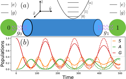
Figure 1: (a) Schematic diagram of the setup described by Eq. II. (b) Solid (dashed) lines show the numerical (effective analytic) populations of the ground (G), symmetric (S), and antisymmetric (A) states for a system with Hamiltonian parameters (and their effective counterparts without dissipation): $\Delta_{0}=-\Delta_{1}=0.02$, $g_{0}=g_{1}=0.02$, $\eta_{0}=\eta_{1}=0.02$, and $\gamma_{d}=2\gamma_{r}=10^{-8}$. Hamiltonian parameters in all figures are expressed as ratios with respect to the dominant energy scale set by $\gamma_{a}=50THz$.

II Theory

We consider a physical setup, illustrated in Fig. 1, consisting of a pair of qubits placed in close proximity to the near-field of a surface plasmon mode supported on a metallic nanowire. Qubit-qubit interactions are thus mediated by a plasmonic boson reservoir. The bare plasmon Hamiltonian is $H_{pls}=\int d\bm{r}\int_{0}^{\infty}d\omega\hbar\omega\hat{a}^{\dagger}(\bm{r},\omega)\hat{a}(\bm{r},\omega)$, where $\hat{a}(\bm{r},\omega)$ and $\hat{a}^{(\dagger)}(\bm{r},\omega)$ are the destruction and creation operators for elementary plasmonic excitations which satisfy bosonic commutation relations. A resonant or near-resonant mode may be treated as an oscillator $H_{pls}=\hbar\omega_{a}\hat{a}^{\dagger}\hat{a}$ with a principal frequency $\omega_{a}$. The qubit Hamiltonian reads $H_{i}=\hbar\omega_{i}\hat{\sigma}_{i}^{+}\hat{\sigma}_{i}^{-}$, where $i=0,1$ indexes the emitters which are modeled as two level systems with $\hat{\sigma}_{i}^{\pm}$ being the Pauli ladder operators, $\hat{\sigma}^{\pm}=\hat{\sigma}^{x}\pm i\hat{\sigma}^{y}=|{e}\rangle\langle{g}|(|{g}\rangle\langle{e}|)$. The qubits could be implemented by a variety of solid state platforms, for example, as semiconductor quantum dotsHanson_RMP ; Stobbe_RMP . We do not restrict ourselves to a specific qubit platform, but note that our results are generally applicable given appropriate plasmonic mode matching, which may be tuned by adjusting the nanowire geometry Chang_2006 ; Dionne_2006 ; Benz_2016 . Defining the plasmonic and TLS dipole operators as $\hat{d}_{a}=\hat{a}^{\dagger}+\hat{a}$ and $\hat{d}_{i}=\hat{\sigma}^{+}_{i}+\hat{\sigma}^{-}_{i}$, the emitter-reservoir coupling is modeled by the interaction $H_{int}=\sum_{i}g_{i}\hat{d}_{a}\cdot\hat{d}_{i}$, where $g_{i}\equiv(\mu_{i}\cdot E_{i})/\hbar$ is the dipole interaction strength in which we have absorbed all physical constants, i.e. the emitter transition dipole moment $\mu_{i}$ and local plasmon electric field magnitude $E_{i}=\sqrt{\frac{\hbar\omega_{a}}{2\epsilon_{0}V}}$ where $V$ is the plasmon mode volume. Plasmonic elements behave as lossy electromagnetic cavities in the both the weak and strong QED regimes Ginzburg_Review ; Hummer_2013 ; Benz_2016 ; Chikkaraddy_2016 ; santhosh2016vacuum ; Akselrod_2014 . Finally, $H_{D}=-\sum_{i}(\eta_{i}e^{i\Omega_{i}t}\hat{\sigma}^{+}_{i}+H.c.)-(\eta_{a}e^{i\Omega_{a}t}\hat{a}^{\dagger}+H.c.)$ models transitions being driven by external fields with amplitudes $\eta_{i(a)}$ and frequencies $\Omega_{i(a)}$. Transforming to the co-rotating reference frame, with detunings $\Delta_{i(a)}=\hbar(\omega_{i(a)}-\Omega_{i(a)})$, and applying the rotating wave approximation, the total Hamiltonian becomes,

$$H_{tot} = \sum_{i=0,1}\left[\Delta_{i}\hat{\sigma}^{+}_{i}\hat{\sigma}^{-}_{i}-\eta_{i}\hat{d}_{i}-g_{i}(\hat{\sigma}^{+}_{i}\hat{a}+\hat{\sigma}^{-}_{i}\hat{a}^{\dagger})\right]$$

$$+ \Delta_{a}\hat{a}^{\dagger}\hat{a}-\eta_{a}\hat{d}_{a}.$$

Dissipation is modeled by treating the dynamics within the Lindblad master equation formalism,

$$\dot{\rho}=-i\left[H_{tot},\rho\right]+\sum_{k}\gamma_{k}(L_{k}\rho L_{k}^{\dagger}-\frac{1}{2}\{L_{k}^{\dagger}L_{k},\rho\})$$ (2)

where we have take $\hbar=1$ and the $L_{k}$ operators model various dissipative channels. Specifically, we consider the following channels: (i) plasmonic relaxation $L_{a}\equiv\hat{a}$ at a rate $\gamma_{a}\leq 50\text{THz}$Rod_ACS , (ii) emitter relaxation $L_{r,i}\equiv\hat{\sigma}_{i}^{+}$ at a rate $\gamma_{r}=2.5\text{MHz}$, and (iii) emitter dephasing $L_{d,i}\equiv\hat{\sigma}_{i}^{z}$ at a rate $\gamma_{d}=5\text{MHz}$. Later we numerically solve Eq. 2 in full to validate anti-bunching and concurrence phenomenon in a wide range of parameter regimes. However, we first derive an effective model to develop our intuition of the dynamics.

III Two-qubit effective dynamics

Let us now illustrate the dissipative flow dynamics for two qubits coupled through a common bosonic reservoir. Both the effective model and our exact numerical calculations will identify the anti-symmetric singlet state $|{A}\rangle=|{eg}\rangle-|{ge}\rangle$ as a fixed point for the dynamical evolution in the parameter regimes highlighted below. For our effective model, we work in the weak coupling regime defined by $g_{0},g_{1},\eta_{0},\eta_{1}\ll\gamma_{a}$, where $\gamma_{a}$ is the rate for the relaxation channel taken with the relaxation timescale $\tau_{a}=1/(\pi*\gamma_{a})\sim 6fs$. In this work we stay within this approximation so all energy and time scales are given as dimensionless ratios of $\gamma_{a}$. Still, the reservoir dynamics enables coherent communication channel between the distant qubits. As we now show, the system may be guided into the decoherence free subspace $|{A}\rangle$ by varying the qubits detunings and drivings in Eq. II, or equivalently, by driving the bosonic reservoir Hou_15 .

The effective qubit dynamics is found by the following adiabatic elimination procedureHou_15 . From Eqs. II and 2 the Heisenberg equations of motion for the field operators are

$$\dot{\sigma}^{z}_{i} = i\left[2g_{i}(\sigma^{+}_{i}a-\sigma^{-}_{i}a^{\dagger})+2\eta_{i}(\sigma^{+}_{i}-\sigma^{-}_{i})\right]$$

$$- \gamma_{i}(\mathbb{I}-\sigma_{z})+f^{z}_{i}$$

$$\dot{\sigma}^{-}_{i} = -i\left[\Delta_{i}\sigma^{-}_{i}+(g_{i}a+\eta_{i})\sigma^{z}_{i}\right]-\gamma_{i}\sigma^{-}_{i}/2+f^{-}_{i}$$

$$\dot{a} = i\left[\eta_{a}-\Delta_{a}a+g_{0}\sigma^{-}_{0}+g_{1}\sigma^{-}_{1}\right]-\gamma_{a}a/2+f_{a},$$

with fluctuation operators $f^{z}_{i},f^{-}_{i},f_{a}$ representing higher order processes Hou_15 . Making the semi-classical approximation that expectation values for the fluctuation operators vanish, we decouple the expectation values of the qubits and the bosonic mode. For slowly varying $\langle{a}\rangle$, valid in the case of weak coupling and drivings, we may set $\dot{a}=0$ and substitute the resulting expression into the the first two lines of Eq. III. This gives us the adiabatic Heisenberg equations of motion, which can in turn be viewed as arising from an effective two qubit Hamiltonian with non-local dissipation terms. The effective Hamiltonian, $H_{qb}=\sum_{i}\left[\tilde{\Delta}_{i}\hat{\sigma}^{+}_{i}\hat{\sigma}^{-}_{i}-\tilde{\eta}_{i}\hat{d}_{i}\right]-\tilde{g}(\hat{\sigma}^{+}_{0}\hat{\sigma}^{-}_{1}+\hat{\sigma}^{+}_{1}\hat{\sigma}^{-}_{0})$, is defined in terms of the following couplings: (i) effective local detunings $\tilde{\Delta_{i}}=\Delta_{i}-g_{i}^{2}\Delta_{a}/Z$, (ii) effective driving fields $\tilde{\eta_{i}}=\eta_{i}+g_{i}\Delta_{a}\eta_{a}/Z$, and (iii) effective inter-qubit coupling $\tilde{g}=g_{0}g_{1}\Delta_{a}/Z$, where $Z=(\gamma_{a}/2)^{2}+\Delta_{a}^{2}$. The effective dissipations are described by $\sum_{ij=0,1}\tilde{\gamma}_{ij}/2\left[2\sigma^{-}_{i}\rho\sigma^{+}_{j}-\{\sigma^{+}_{j}\sigma^{-}_{i},\rho\}\right]$, with single qubit relaxations occurring at a renormalized rate $\tilde{\gamma}_{ii}=\gamma_{i}+g_{i}^{2}\gamma_{a}/Z$ and collective reservoir mediated relaxations occurring at the rate $\tilde{\gamma}_{ij}=g_{0}g_{1}\gamma_{a}/Z$. Transforming to the Dicke basis, $|{E}\rangle=|{ee}\rangle\equiv|{s=1,m=1}\rangle$, $|{S}\rangle=|{eg}\rangle+|{ge}\rangle$, $|{A}\rangle=|{eg}\rangle-|{ge}\rangle$, $|{G}\rangle=|{gg}\rangle$, and defining the effective (anti)symmetric drivings $\eta_{\pm}=(\tilde{\eta}_{0}\pm\tilde{\eta}_{1})/\sqrt{2}$ and energies $\Delta_{\pm}=(\tilde{\Delta}_{0}\pm\tilde{\Delta}_{1})/2$. Note that $|{A}\rangle$ is the part of the two-qubit space while $|{G}\rangle,|{S}\rangle,|{E}\rangle$ define the triplet basis vectors defined by angular momentum eigenvalues $m=-1,0,1$ respectively.

The Hamiltonian now reads

$$H_{D} = \Delta_{E}|{E}\rangle\langle{E}|+\Delta_{S}|{S}\rangle\langle{S}|+\Delta_{A}|{A}\rangle\langle{A}|$$

$$+ \Delta_{-}(|{A}\rangle\langle{S}|+|{S}\rangle\langle{A}|)$$

$$- \eta_{-}(|{S}\rangle\langle{G}|+|{S}\rangle\langle{E}|+H.c)$$

$$- \eta_{+}(|{A}\rangle\langle{G}|-|{A}\rangle\langle{E}|+H.c).$$

where $\Delta_{E}=2\Delta_{+}$, $\Delta_{S}=\Delta_{+}+\tilde{g}$, and $\Delta_{A}=\Delta_{+}-\tilde{g}$.

As a special case, we take anti-symmetric detunings and identical drivings, thus reducing the effective parameters to $\tilde{\Delta_{i}}=\Delta_{i},\;\tilde{\eta_{i}}=\eta_{i},\;\tilde{g}=0,\;\tilde{\gamma}_{ii}=\gamma_{i}+4g_{i}^{2}/\gamma_{a},$ and $\tilde{\gamma_{ij}}=4g_{0}g_{1}/\gamma_{a}$. The resulting pure state populations, e.g. with $\rho(0)=|{G}\rangle\langle{G}|$, oscillate with an effective two qubit Rabi frequency $\Omega=\sqrt{(\Delta/2)^{2}+\eta^{2}}$ as $\rho_{E}(t)=\left(\Delta^{2}+\eta^{2}\cos(2t\Omega)-\Omega^{2}\right)^{2}/4\Omega^{4},\;\rho_{S}(t)=\eta^{2}\sin^{2}(2t\Omega)/2\Omega^{2},\;\rho_{A}(t)=2\Delta^{2}\eta^{2}\sin^{4}(t\Omega)/\Omega^{4},\;\rho_{G}(t)=\left(\Delta^{2}+\eta^{2}\cos(2t\Omega)+\Omega^{2}\right)^{2}/4\Omega^{4}$, and are illustrated by the dashed lines in Fig. 1.

The solid populations in Fig. 1 are calculated by numerically solving Eq. 2 for the full system and can be understood as follows. As discussed above, the excited state $|{E}\rangle$ relaxes to the singly excited state $|{eg(ge)}\rangle$ at a rate $\tilde{\gamma}_{00(11)}$. However, in the Dicke basis, relaxation from the bi-excited state to the symmetric (antisymmetric) state occurs at the rate $\gamma_{S(A)}=\sum_{i}\tilde{\gamma}_{ii}/2\pm\gamma_{ij}$. Ignoring Hamiltonian dynamics for the moment, the populations are coupled as $\dot{\rho}_{SS}=(\rho_{EE}-\rho_{SS})\gamma_{S}$ and $\dot{\rho}_{AA}=(\rho_{EE}-\rho_{AA})\gamma_{A}$. Thus, the solid lines in Fig.1 and the eventual steady states, are driven by symmetric pumping described by Eq. III augmented by super- and sub-radiant dissipation from the states $|{S}\rangle,$ and $|{A}\rangle$ respectively. As discussed below, the entangled state $|{A}\rangle$ is a fixed point solution to these dynamics.

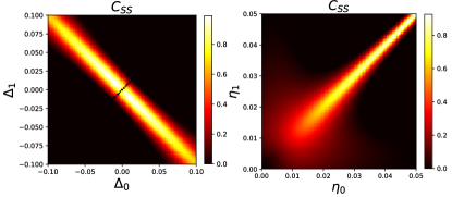
Figure 2: Heat map of steady state concurrence $C_{ss}$ as a function of (left) qubit detunings $\Delta_{0,1}$ with equal qubit drivings $\eta_{0}=\eta_{1}=0.05$ and (right) qubit driving amplitudes $\eta_{0,1}$ with asymmetric qubit detunings $\Delta_{0}=-\Delta_{1}=0.01$. Symmetric drivings and couplings with anti-symmetric detunings yields near unity concurrence steady states $\rho_{ss}\approx|{A}\rangle\langle{A}|$. Parameters common to both panels are coupling strengths $g_{0}=g_{1}=0.05$ and plasmon detuning and driving $\Delta_{a}=\eta_{a}=0$.

We now explore steady state characteristics as a function of the parameter space defined in Eq. II. Fixed point entanglement is characterized by Wooter’s concurrence $C$ Wooters_98 . The concurrence of a two qubit state $\rho$ is $C(\rho)=\max\{0,\lambda_{1}-\lambda_{2}-\lambda_{3}-\lambda_{4}\}$ where $\lambda_{j}$ are the sorted eigenvalues of $\rho\tilde{\rho}$, with the spin-flipped conjugate state $\tilde{\rho}=\sigma^{y}_{1}\sigma^{y}_{2}\rho^{*}\sigma^{y}_{2}\sigma^{y}_{1}$. $C$ ranges between $0$, for product states, and $1$, for maximally entangled states. As indicated by our earlier discussion and illustrated in Fig. 2, unit concurrence is readily achievable for systems with approximately equal couplings and driving fields as well as approximately anti-symmetric qubit detuning. In all cases, the pair of qubits evolves to the anti-symmetric entangled state $|{A}\rangle$ Cano_2011 ; Hou_15 .

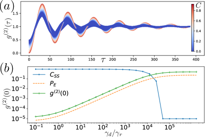
Figure 3: The steady state $g^{(2)}(\tau)$ correlation function as driving amplitudes $\eta_{1}=0.05$ and $\eta_{0}$ varies across $\left[0.04,0.06\right]$. The blue traces in panel (a) correspond to statistical mixtures of $|{gg}\rangle$ and $|{eg(ge)}\rangle$ depending on the circle endpoints. These states showing a $g^{(2)}(0)=0.5$ and correspond to general mixed states. Over this range the concurrence evolves (see colorbar labeled by $C$) from $0$, where $g^{(2)}(0)=1/2$, to $1$, where $g^{(2)}(0)=0$. Other Hamiltonian parameters, as ratios of $\gamma_{a}$, are $\Delta_{0}=-\Delta_{1}=0.02$, $g_{0}=g_{1}=0.05$, and $\eta_{1}=0.05$. $\tau$ is presented in units of $1/(\pi*\gamma_{a})\approx 6fs$.

IV $g^{(2)}(\tau)$ as an entanglement witness

We now investigate the use of the second order temporal correlation function to quantify entanglement generation in our system. Entanglement is typically validated by an ensemble of computational basis state measurements that are classically post-processed to either perform state tomographyPoyatos_97 ; Chuang_97 or demonstrate a quantum inequality violationBell ; CHSH . Tomographic state readout has been successfully performed for dissipatively entangled trapped ions Lin_Nature using specialized readout mechanisms. However, for nascent plasmonic technologies, it is worthwhile to develop simple experimental signatures consistent with entangled states, without the complicated readout electronics needed to perform full state tomography.

In this context, anti-bunching in $g^{(2)}(\tau)$ of emitted light has been suggested as an alternative entanglement signature Cano_2011 ; Zheng_2013 ; Thakkar_2015 . Below we confirm that the second order correlation function successfully discriminates between entangled, arising in the form $|{A}\rangle$, and unentangled steady states generated by our protocol. Importantly, anti-bunching by itself is not conclusive evidence of entanglement between qubits with a shared dissipative pathway. For instance, if both qubits were not well-coupled to the same plasmonic mode, steady-state entanglement would not be generated, but each qubit would exhibit anti-bunching on a timescale determined by the lifetime of the qubit. By considering the anti-bunching dynamics, it is possible to distinguish anti-bunching due to individual uncoupled emitters and anti-bunching due to dissipative, driven, entanglement between qubits coupled to a shared plasmonic reservoir.

The second order correlation function measures the degree to which a system is temporally correlated. For stationary processes invariant under time translation, as is the case for steady states, the correlation function is defined as

$$g^{(2)}(\tau)=\frac{\langle a^{\dagger}(t)a^{\dagger}(t+\tau)a(t+\tau)a(t)\rangle}{\langle a^{\dagger}(t)a(t)\rangle^{2}}.$$ (5)

In the context of quantum optics, $g^{(2)}(\tau)$ has the simple and intuitive interpretation of the normalized probability that two photons, whose emission times differ by $\tau$, are detected at a point in space. A Hanbury Brown-Twiss (HBT) interferometer HBT can be used to measure this quantity. In a modern HBT interferometer, a 50/50 beamsplitter is used to send a light source to a pair of single photon counting detectors, and high speed electronics tag the arrival times of photons at each detector, with temporal resolution as fast as 1 picosecond.

In order to calculate $g^{(2)}(\tau)$, let us now combine continuous time evolution with a discrete quantum jump model. Consider a steady state $\rho_{ss}$ of Eq. 2, whose concurrence is plotted in Fig. 2, which spontaneously emits a single photon from either qubit. An emission event originating from the $i^{\text{th}}$ qubit corresponds mathematically to the application of a destruction operator $\sigma^{-}_{i}$ which projectively maps the post-emission state to $\rho_{i}(0)=\hat{\sigma}_{i}^{(-)}\rho_{ss}\hat{\sigma}_{i}^{(+)}/\text{Tr}\left[\hat{\sigma}_{i}^{(-)}\rho_{ss}\hat{\sigma}_{i}^{(+)}\right]$. Defining $\rho_{i}(\tau)$ as $\rho_{i}(0)$ evolved from $t=0$ to $t=\tau$ according to Eq. 2, the probability for a second emission from the $j$th qubit at time $\tau$ is then $\text{Tr}\left[\hat{n}_{j}\rho_{i}(\tau)\right]$, where $\hat{n}_{j}=\hat{\sigma}_{j}^{(+)}\hat{\sigma}_{j}^{(-)}$ is the qubit number operator. Tracing over all emission configurations gives us the correlation function

$$g^{(2)}(\tau)=\sum_{ij}\text{Tr}\left[\hat{n}_{j}\rho_{i}(\tau)\right].$$ (6)

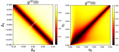
Figure 4: Zero-delay correlations $g^{(2)}(0)$ as a function of (left) qubit detunings $\Delta_{0,1}$ and (right) qubit drive amplitudes $\eta_{0,1}$ using parameters reported in Fig. 2. Dark bands, which overlap strongly with the high concurrence regions, denote parameter regimes for which anti-bunching is present.

Fig. 3 panel (a) illustrates the behavior of $g^{(2)}(\tau)$ when the driving amplitude $\eta_{0}$ varies across $\left[0.04,0.06\right]$. Across this range, the concurrence varies from 0 to 1, and back to 0, as denoted by the color of the curves (also see Fig. 2). At unity concurrence we observe that $g^{(2)}(0)=0$, while for unentangled states, marked by vanishing concurrence, the zero-delay correlations saturate to $g^{(2)}(0)\sim 0.5$. Generally, this correlated anti-bunching signature appears for all dissipatively generated entangled steady states, as can be seen by comparing Figs. 2,4.

It is interesting and necessary to study the effects of generic decoherence with respect to entanglement generation and anti-bunching. For example, we consider dephasing noise which is modeled by the presence of dephasing channels acting locally on each qubit. In Fig. 3 panel (b) we vary the strength of the dephasing noise with respect to the relaxation rate and plot the steady state concurrence, zero-delay signal and population of the dually excited state $|{E}\rangle=|{ee}\rangle$

We emphasize that the observation of an anti-bunching dip is not a general entanglement metric for arbitrary quantum states. However it is a universal feature shared by sub-radiance generated entangled steady states in our setup. It is worth noting that anti-bunching is routinely observed in experiments involving single quantum emitters. The anti-bunching from single quantum emitters is rooted in the fact that after emitting a photon the emitter relaxes to its ground state and cannot source another photon without some time passing for the emitter to become excited again. For single quantum emitters, the anti-bunching dip width is proportional to the bare emitter decay rate ($\gamma_{r}$). Below we discuss how the width of the anti-bunching emanating from a pair of emitters, which are coupled by a common plasmonic reservoir, is many orders of magnitude smaller than a signal being sourced by a single quantum emitter.

Note that the robustness of the anti-bunching signal is rooted in the fact that, similar to the single emitter case, a single quantum is shared between two qubits in the form of the state $|{A}\rangle$. Anti-bunching could also be caused by product states sharing a single quantum, e.g. $|{eg}\rangle$ or $|{ge}\rangle$, but these are unstable under the dynamics considered and the timescales would be quite different as already mentioned. Further, $g^{(2)}(\tau)$ is unaffected by states including statistical mixtures of $|{G}\rangle$ (which don’t contribute any emissions), while the bi-excited state $|{E}\rangle$ may generate two emission events with a small delay with high probability. These dual emissions destroy the anti-bunching signal. Anti-bunching is therefore maximal in our setup for the only stable single excitation subspace: $|{A}\rangle$.

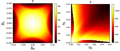
Figure 5: Oscillation timescales for anti-bunching signal as a function of (left) qubit detunings $\Delta_{0,1}$ and (right) qubit drive amplitudes $\eta_{0,1}$. Timescales reported are in units of $T=1/(\pi*\gamma_{a})\approx 6fs$ with remaining parameters as in Fig. 2. Entangled region around $\eta_{0}=\eta_{1}=0.03$ displays a characteristic bunching timescale $T_{AB}\sim 10ps$.

While anti-bunching is an attractive entanglement signature due to its simplicity, its observation is non-trivial due to the fast time-scales inherited from the plasmonic reservoir. After each radiative decay event, the two qubit system flows back to its steady state solution as described earlier. Hence the width of the $g^{(2)}(0)$ anti-bunching dip is inversely proportional to the population oscillation Rabi frequency $\Omega$. Tunable driving frequencies are therefore critical to observing anti-bunching on experimentally accessible timescales. While nonlinear mixing with femtosecond laser sources could enable the detection of sub-picosecond dynamics in $g^{(2)}(\tau)$, conventional HBT interferometry is limited by the $1$ ps temporal resolution of state-of-the-art time tagging electronics. To that end, we numerically calculate the oscillation timescales by Fourier transforming the $g^{(2)}(\tau)$ signal into the frequency domain and identifying the characteristic driving frequency, which fixes the anti-bunching timescale. The timescales are provided in the Fig. 5 color-maps, as a function of detuning and driving amplitudes, with normalized time in units of $T=1/(\pi*\gamma_{a})\approx 6fs$ reported in the color legend. Anti-bunching timescales in the $\sim 10ps$ range for entangled states are easily experimentally realizable, e.g. for small driving fields around $\eta_{0}=\eta_{1}\approx 0.03$. Notably, these timescales are much shorter than the lifetimes of typical qubits. For instance NV centers in diamond have lifetimes of order 10-30 ns doherty2013nitrogen .

V Conclusion and discussion

In this letter we have examined the entanglement characteristics of steady states generated by a pair of qubits subject to a dissipative plasmonic reservoir. We have found that maximally entangled steady states are routinely achievable by appropriately tuning qubit detunings, couplings and driving frequencies. Further, the entanglement was found to be robust against small perturbations in the tuning parameters, which need only be approximately symmetric (couplings, drivings) or anti-symmetric (detunings) in order to generate high concurrence states.

We have also examined entanglement detection by an anti-bunching signature in the second order correlation function that is routinely measured by means of a Hanbury Brown-Twiss interferometer. By correlating this effect with the steady state concurrence, we have analyzed how the correlation function at zero-delay may serve as a robust entanglement signature for dissipating coupled qubit systems. Importantly, we have also demonstrated that dynamics driven by weak fields allows the anti-bunching signature to persist on $\mathcal{O}(ps)$ timescales that pave the way to experimental detection using currently available experimental techniques. This robustness against microscopic perturbations and unentangled fixed point states cements the $g^{(2)}(\tau)$ correlation function as a simple and practical measure of steady state entanglement generation.

Acknowledgements.— The authors thank F. Mohiyaddin for discussions and careful reading of the manuscript. E. D. acknowledges support from the Intelligence Community Postdoctoral Research Program. Research sponsored by the Intelligence Community Postdoctoral Research Fellowship and the Laboratory Directed Research and Development Program of Oak Ridge National Laboratory, managed by UT-Battelle, LLC, for the U.S. Department of Energy. This manuscript has been authored by UT-Battelle, LLC, under Contract No. DE- AC0500OR22725 with the U.S. Department of Energy.

References

- (1) M. A. Nielsen and I. L. Chung, Quantum Computation and Quantum Information, Cambridge University Press (2010)
- (2) B. M. Terhal, “Quantum error correction for quantum memories”, Rev. Mod. Phys. 87, 307 (2015)
- (3) “Fault-tolerant quantum computation with constant error”, D. Aharonov and M. Ben-Or, Proc. 29th Ann. ACM Symp. on Theory of Computation, ACM, New York, (1998)
- (4) P. W. Shor, Phys. Rev. A 52, R 2493(R) (1995)
- (5) A. R. Calderbank, E. M Rains, P. W. Shor, and N. J. A. Sloane, “Quantum Error Correction via Codes over GF(4)” IEEE Trans. Inform. Theory, 44 1369-1387 (1998).
- (6) R. Laflamme, C. Miquel, J. P. Paz, and W. Zurek, “Perfect Quantum Error Correcting Code” Phys. Rev. Lett. 77, 198 (1996)
- (7) A. M. Steane, “Error correcting codes in quantum theory” Phys. Rev. Lett. 77, 793-797 (1996)
- (8) D. Gottesman, Caltech Thesis, arXiv:quant-ph/9705052, (1997)
- (9) A. Y. Kitaev, “Fault-tolerant quantum computation by anyons” Annals of Physics 303 2-30 (2003)
- (10) “Dynamical Decoupling of Open Quantum Systems”, L. Viola, E. Knill, S. Lloyd, Phys. Rev. Lett. 82, 2417 (1999)
- (11) “Quantum feedback control and classical control theory”, A. C. Doherty, S. Habib, K. Jacobs, H. Mabuchi, and S. M. Tan, Phys. Rev. A 62, 012105 (2000)
- (12) “Quantum control theory and applications: A survey”, D. Dong, I. R. Petersen, IET Control Theory & Applications, 4, 12, (2010)
- (13) “Quantum computation and quantum-state engineering driven by dissipation,” F. Verstraete, M. M. Wolf, and J. I. Cirac, Nat. Phys. 5, 633 (2009)
- (14) “Driving two atoms in an optical cavity into an entangled steady state using engineered decay”, F. Reiter, M. J. Kastoryano, A. S. Sorensen, New Journal of Physics 14 053022 (2012)
- (15) “Precisely Timing Dissipative Quantum Information Processing,” M. J. Kastoryano, M. M. Wolf, and J. Eisert, Phys. Rev. Lett. 110, 110501 (2013)
- (16) “Dissipative production of a maximally entangled steady state of two quantum bits”, Y. Lin, J. P. Gaebler, F. Reiter, T. R. Tan, R. Bowler, A. S. Sorensen, D. Leibfried, and D. J. Wineland, Nature 504, 415-418 (2013)
- (17) “Dissipatively driven entanglement of two macroscopic atomic ensembles,” C. A. Muschik, E. S. Polzik, and J. I. Cirac, Phys. Rev. A 83, 052312 (2011)
- (18) “Entanglement generated by dissipation and steady state entanglement of two macroscopic objects”, H. Krauter, C. A. Muschik, K. Jensen, W. Wasilewski, J. M. Petersen, J. Ignacio Cirac, E. S. Polzik, Phys. Rev. Lett. 107, 080503 (2011)
- (19) “Comparing and Combining Measurement-Based and Driven-Dissipative Entanglement Stabilization” Y. Liu, S. Shankar, N. Ofek, M. Hatridge, A. Narla, K. M. Sliwa, L. Frunzio, R. J. Schoelkopf, and M. H. Devoret, Phys. Rev. X 6] 011022 (2016)
- (20) “Quantum Plasmonics” M. S. Tame, K. R. McEnery, S. K. Ozdemir, J. Lee, S. A. Maier, and M. S. Kim, Nature Physics 9, 329?340 (2013)
- (21) “Cavity quantum electrodynamics in application to plasmonics and metamaterials”, P. Ginzburg, Reviews in Physics 1 120-139 (2016)
- (22) “Plasmon-assisted transmission of entangled photons”, E. Altewischer, M. P. van Exter and J. P. Woerdman, Nature 418, 304-306 (18 July 2002)
- (23) “Extraordinary Optical Transmission of Multimode Quantum Correlations via Localized Surface Plasmons”, B. J. Lawrie, P. G. Evans, and R. C. Pooser, Phys. Rev. Lett. 110, 156802, (2013)
- (24) “Toward quantum plasmonic networks”, M. W. Holtfrerich, M. Dowran, R. Davidson, B. J. Lawrie, R. C. Pooser, and A. M. Marino, Optica Vol. 3, Issue 9, pp. 985-988 (2016)
- (25) “Quantum plasmonic sensing”, W. Fan, B. J. Lawrie, and R. C. Pooser, Phys. Rev. A 92, 053812 (2015)
- (26) “Plasmonic Trace Sensing below the Photon Shot Noise Limit”, R. C. Pooser and B. Lawrie, ACS Photonics, 3 (1), pp 8-13 (2016)
- (27) “Probing the mechanisms of large Purcell enhancement in plasmonic nanoantennas”, G. M. Akselrod, et. al., Nature Photonics, 8, 835–840, (2014).
- (28) “Vacuum Rabi splitting in a plasmonic cavity at the single quantum emitter limit”, K. Santhosh, O. Bitton, L. Chuntonov, and G. Haran, Nature Communications, 7, 11823, (2016).
- (29) “Single-molecule strong coupling at room temperature in plasmonic nanocavities”, R. Chikkaraddy, et. al., Nature 535, 7610 (2016).
- (30) “Weak and strong coupling regimes in plasmonic QED”, T. Hummer, F. J. Garcia-Vidal, L. Martin-Moreno, and D. Zueco, Phys. Rev. B 87, 115419 (2013)
- (31) “Surface plasmons in a metal nanowire coupled to colloidal quantum dots: Scattering properties and quantum entanglement”, G.-Y. Chen, N. Lambert, C.-H. Chou, Y.-N. Chen, and F. Nori, Phys. Rev. B 84, 045310 (2011)
- (32) “Multifrequency multi-qubit entanglement based on plasmonic hot spots”, J. Ren, T. Wu, and X. Zhang, Sci. Rep. 5, 13941 (2015)
- (33) “Nanoshell-mediated robust entanglement between coupled quantum dots’, J. Hakami and M. S. Zubairy, Phys. Rev. A 93, 022320 (2016)
- (34) “Dissipative dynamics of a solid-state qubit coupled to surface plasmons: From non-Markov to Markov regimes”, A. Gonzalez-Tudela, F. J. Rodr guez, L. Quiroga, and C. Tejedor, Phys. Rev. B 82, 115334 (2010)
- (35) “Robust-to-loss entanglement generation using a quantum plasmonic nanoparticle array”, C. Lee, M. Tame, C. Noh, J. Lim, S. A. Maier, J. Lee, and D. G. Angelakis, New Jour. Phys., Vol. 15, (2013)
- (36) “Transient and steady-state entanglement mediated by three-dimensional plasmonic waveguides”, S. A. H. Gangaraj, A. Nemilentsau, G. W. Hanson, and S. Hughes, Optics Express Vol. 23, Issue 17, pp. 22330-22346 (2015)
- (37) “Entanglement of two qubits mediated by a localized surface plasmon”, K. V. Nerkararyan and S. I. Bozhevolnyi, Phys. Rev. B 92, 045410 (2015)
- (38) “Entanglement of two, three, or four plasmonically coupled quantum dots”, M. Otten, R. A. Shah, N. F. Scherer, M. Min, M. Pelton, and S. K. Gray, Phys. Rev. B 92, 125432 (2015)
- (39) “Origins and optimization of entanglement in plasmonically coupled quantum dots”, M. Otten, J. Larson, M. Min, S. M. Wild, M. Pelton, and S. K. Gray, Phys. Rev. A 94, 022312 (2016)
- (40) “Dissipation-driven generation of two-qubit entanglement mediated by plasmonic waveguides”, D. Martin-Cano, A. Gonzalez-Tudela, L. Martin-Moreno, F. J. Garcia-Vidal, C. Tejedor, and E. Moreno, Phys. Rev. B 84, 235306 (2011)
- (41) “Entanglement of Two Qubits Mediated by One-Dimensional Plasmonic Waveguides” A. Gonzalez-Tudela, D. Martin-Cano, E. Moreno, L. Martin-Moreno, C. Tejedor, and F. J. Garcia-Vidal, Phys. Rev. Lett. 106, 020501 (2011)
- (42) “Dissipation-driven entanglement between qubits mediated by plasmonic nanoantennas,” J. Hou, K. Slowik, F. Lederer, and C. Rockstuhl, Phys. Rev. B 89, 235413 (2014)
- (43) R. Hanson, L. P. Kouwenhoven, J. R. Petta, S. Tarucha, and L. M. K. Vandersypen, “Spins in few-electron quantum dots”, Rev. Mod. Phys. 79, 1217 (2007).
- (44) P. Lodahl, S. Mahmoodian, and S. Stobbe, “Interfacing single photons and single quantum dots with photonic nanostructures”, Rev. Mod. Phys. 87, 347 (2015).
- (45) “Quantum optics with surface plasmons”, D. E. Chang, A. S. S rensen, P. R. Hemmer, and M. D. Lukin, Phys. Rev. Lett, 97, 5, (2006).
- (46) “Plasmon slot waveguides: Towards chip-scale propagation with subwavelength-scale localization”, J. A. Dionne, L. A. Sweatlock, H. A. Atwater, and A. Polman, Phys. Rev. B 73, 035407 (2006).
- (47) “Single-molecule optomechanics in “picocavities” ” F. Benz, et. al., Science, 354, 6313, (2016).
- (48) “Ultrafast Plasmonic Control of Second Harmonic Generation”, R. B. Davidson II, A. Yanchenko, J. I. Ziegler, S. M. Avanesyan, B. J. Lawrie, and R. F. Haglund Jr. ACS Photonics, 3 (8), pp 1477?1481 (2016)
- (49) “Entanglement of Formation of an Arbitrary State of Two Qubits”, W. K. Wooters, Phys. Rev. Lett. 80 2245 (1998)
- (50) “The nitrogen-vacancy colour centre in diamond”, M.W. Doherty, N.B Manson, P. Delaney, F. Jelezko, J. Wrachtrip, and CL Hollenberg, Phys. Rep. 528 1-45 (2013)
- (51) J. F. Poyatos , J. I. Cirac, P. Zoller, “Complete Characterization of a Quantum Process: The Two-Bit Quantum Gate”, Phys. Rev. Lett. 78 390 (1997).
- (52) I. L. Chuang and M. A. Nielsen “Prescription for experimental determination of the dynamics of a quantum black box”, Journal of Modern Optics, 44 11-12, 2455-2467 (1997).
- (53) “On the EPR paradox”, J. S. Bell, Physics 1, 195 (1964).
- (54) “Proposed Experiment to Test Local Hidden-Variable Theories”, J. F. Clauser, M. A. Horne, A. Shimony, and R. A. Holt, Phys. Rev. Lett. 23, 880 (1969).
- (55) “Persistent Quantum Beats and Long-Distance Entanglement from Waveguide-Mediated Interactions”, H. Zheng and H. U. Baranger, PRL 110, 113601 (2013)
- (56) “Quantum Beats from Entangled Localized Surface Plasmons”, N. Thakkar, C. Cherqui, and D. J. Masiello, ACS Photonics, 2 (1), pp 157-164 (2015)
- (57) “A Test of a New Type of Stellar Interferometer on Sirius”, R. Hanbury Brown and R. Q. Twiss Nature 178, 1046 - 1048 (1956)