Halo Histories vs. Galaxy Properties at z=0, III:
The Properties of Star-Forming Galaxies
Abstract
We measure how the properties of star-forming central galaxies correlate with large-scale environment, , measured on Mpc scales. We use galaxy group catalogs to isolate a robust sample of central galaxies with high purity and completeness. The galaxy properties we investigate are star formation rate (SFR), exponential disk scale length , and Sersic index of the galaxy light profile, . We find that, at all stellar masses, there is an inverse correlation between SFR and , meaning that above-average star forming centrals live in underdense regions. For and , there is no correlation with at , but at higher masses there are positive correlations; a weak correlation with and a strong correlation with . These data are evidence of assembly bias within the star-forming population. The results for SFR are consistent with a model in which SFR correlates with present-day halo accretion rate, . In this model, galaxies are assigned to halos using the abundance matching ansatz, which maps galaxy stellar mass onto halo mass. At fixed halo mass, SFR is then assigned to galaxies using the same approach, but is used to map onto SFR. The best-fit model requires some scatter in the -SFR relation. The and measurements are consistent with a model in which both of these quantities are correlated with the spin parameter of the halo, . Halo spin does not correlate with at low halo masses, but for higher mass halos, high-spin halos live in higher density environments at fixed . Put together with the earlier installments of this series, these data demonstrate that quenching processes have limited correlation with halo formation history, but the growth of active galaxies, as well as other detailed galaxies properties, are influenced by the details of halo assembly.
keywords:
cosmology: observations—galaxies:clustering — galaxies: evolution1 Introduction
This is the third installment of a series of papers focused on possible connections between the properties of present-day galaxies and the evolutionary histories of the halos in which those galaxies formed. In each work, we select a sample of ‘central’ galaxies with which to make our comparisons. These galaxies live at the center of distinct halos—these galaxies could also be referred to as ‘field galaxies’—and have not been subjected to the type of physical processes that transform galaxies that have been accreted as satellites onto groups and clusters. In Papers I and II, we investigated the quenched fraction of central galaxies in the SDSS, , comparing various measurements of this quantity to models in which halo formation history is correlated with mean stellar age, known as the age-matching model (Hearin & Watson 2013; Hearin et al. 2015). This model predicts that red-and-dead galaxies live in the oldest halos, while the most active star-formers live in the youngest. In Paper I, we determined that such models predict a dependence of on large-scale density that is inconsistent with observations. At fixed mass, halo clustering depends on halo age, an effect known as assembly bias (Wechsler et al. 2006; Gao & White 2007). Thus, the age-matching model predicts that quiescent central galaxies should predominantly live in dense regions, but will rarely be found in underdense regions. The measurements of Paper I shows essentially no correlation between and density at the halo masses where the age-matching model predicts it to be the strongest.
In Paper II we explored through galactic conformity (see, e.g., Kauffmann et al. 2013; Hearin et al. 2015), once again finding that halo formation has a limited, if any, role in determining whether a galaxy makes the transition from star-forming to quiescence. In this paper, we narrow our sample to only looking at central galaxies that are actively star-forming. Theoretical models of galaxy growth inside halos usually assume some relationship between the properties of disky, active galaxies, and the dark matter halo that surrounds them. We will test several of these assumptions.
In some respects, the correlation between galaxy growth and halo growth is undeniable: larger galaxies live in larger halos. The abundance matching model has been used as a function of redshift to infer the details of this correlation (Conroy & Wechsler 2009; Behroozi et al. 2013b, a; Moster et al. 2013). In all of these models, it is assumed that the baryonic accretion rate onto a halo is proportional to the dark matter accretion rate of that halo. Abundance matching tells one how much the galaxy within a given halo has grown, and with this information one can infer the efficiency of star formation over that time interval. For two halos of the same mass today, the halo that grew the most over that time should have the highest star formation rate. Halo growth rate is tied to closely tied to assembly bias, thus this prediction of the abundance matching ansatz creates testable predictions for the population of central galaxies.
In the canonical picture of galaxy formation in a CDM universe, the properties of disk galaxies are determined by the relationship between dark matter and baryons. Accreted baryons are converted into a disk of cold gas and stars that has an exponential scale length determined by the angular momentum of the dark matter halo, which is aligned and distributed proportionately with the baryonic material (Dalcanton et al. 1997; Mo et al. 1998). Recent cosmological hydrodynamic simulations have found that halo spin is correlated with the size and morphology of the stellar material, but with significant scatter (Teklu et al. 2015; Zavala et al. 2016; Rodriguez-Gomez et al. 2017). Several studies have shown that halo angular momentum (or ‘spin’ for brevity) is another halo property that influences—or is influenced by—the clustering of the halos: higher spin halos live in more dense regions (Gao & White 2007; Bett et al. 2007), giving us the opportunity to test this theory observationally.
Cosmological hydrodynamic simulations demonstrate that merger activity is strongly correlated with the buildup of a central bulge (see, e.g., Brooks & Christensen 2016 and citations therein). The merger rate of dark matter halos depends on large scale density such that more mergers occur in higher density environments. This dependence is not particularly strong—the merger rate increases by a factor of over roughly a factor of 10 in (Fakhouri & Ma 2009). But bulgeless, disk-dominated galaxies in the local universe have most likely experienced the lowest amount of merging in the galaxy population. If so, they should reside in the lowest densities within which such galaxies can be found, making it possible to detect this effect.
The key to all of these supposedly observable trends, as always, is having an unbiased sample of central galaxies. Galaxies that orbit within larger halos as satellites have been subject to a set of physical processes that are distinct from those than can act on central galaxies in the field. As in Papers I and II, we will use group catalogs to identify central galaxies within the full SDSS DR7. The tight correlation between stellar mass and halo mass implies that we can use stellar mass as a reasonable proxy for halo mass. Thus, a pure and complete set of central galaxies at fixed stellar mass is an effective way to examine a set of halos at fixed dark matter mass. In this context, the search for assembly bias is much cleaner and more straightforward.
Throughout, we define a galaxy group as any set of galaxies that occupy a common dark matter halo, and we define a halo as having a mean interior density 200 times the background matter density. For all distance calculations and group catalogs we assume a flat, CDM cosmology of . Stellar masses are in units of .
2 Data, Measurements, and Methods
2.1 NYU Value-Added Galaxy Catalog and Group Catalog
As in Papers I and II, we use the NYU Value-Added Galaxy Catalog (VAGC; Blanton et al. 2005) based on the spectroscopic sample in Data Release 7 (DR7) of the Sloan Digital Sky Survey (SDSS; Abazajian et al. 2009). We use stellar masses from the kcorrect code of Blanton & Roweis (2007), which assumes a Chabrier (2003) initial mass function. Estimates of the specific star formation rates (sSFR) of the VAGC galaxies are taken from the MPA-JHU spectral reductions111http://www.mpa-garching.mpg.de/SDSS/DR7/ (Brinchmann et al. 2004).
The group catalogs are created from volume-limited stellar mass samples. Details of the group finding process can be found in Tinker et al. (2011) and further tested in Campbell et al. (2015). In brief, the group finding algorithm used here is based on that of Yang et al. (2005), in which the full galaxy population can be decomposed into two distinct populations: central galaxies, that exist at the center of a distinct dark matter halo, and satellite galaxies, that orbit within a larger dark matter halo. Each galaxy in the sample is given a probability of being a satellite galaxy, . In our fiducial sample, galaxies with are classified as satellites, while galaxies with are classified as centrals.
In this paper we focus exclusively on central galaxies. Impurities and incompleteness are inevitable consequences of any group-finding process. Using our group finer, the purity of the full sample of central galaxies is around 90%, with a completeness of . However, the purity of the sample of central galaxies has a strong correlation with . The vast majority of central galaxies have , with many being exactly 0. Most incorrectly classified central galaxies—i.e., true satellite galaxies that are labeled as centrals by the algorithm—have in the range . Thus, we can create a ‘pure’ sample of central galaxies by reducing the threshold to . This excludes roughly of classified centrals but reduces the impurity to . Our fiducial results in this paper will use samples of pure central galaxies in order to avoid any bias from including true satellite galaxies in the sample. In Appendix B we demonstrate that our fiducial results are largely unaffected by this choice.
In addition to focusing on central galaxies, we specifically want to investigate the properties of galaxies on the star-forming main sequence (SFMS). The SFMS is characterized by a power-law dependence of star-formation rate (SFR) and , with a lognormal scatter of roughly 0.3 dex around the mean SFR (Noeske et al. 2007). Dividing a sample of galaxies into star forming and quiescent usually involves splitting a bimodal distribution at the minimum between the two modes of the galaxy distribution. However, there are galaxies that are on either side of that division that are not canonical star forming or quiescent objects, but rather in the process of migrating from the former to the latter. We call these transitioning galaxies. The relative height of this ‘green valley’ to the peaks contains information about the quenching timescale of galaxies. Using this information, Wetzel et al. (2013) and Hahn et al. (2017) find that satellite galaxies and central galaxies typically spend and Gyr in this migration, respectively.
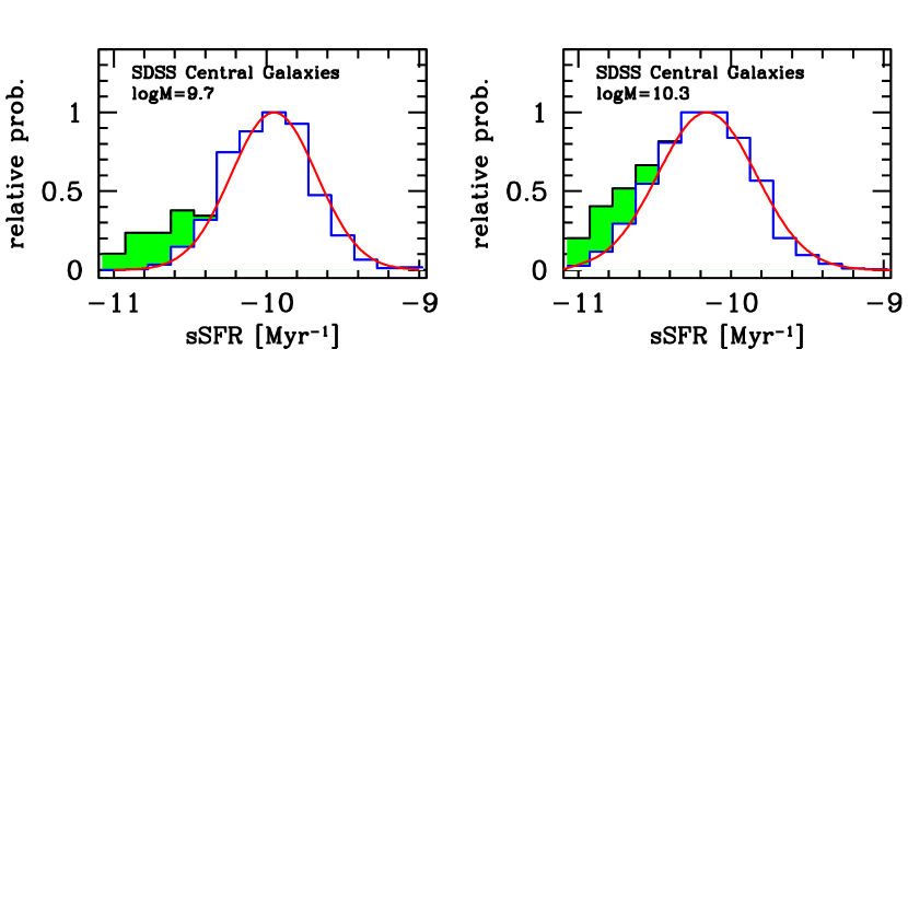
Identifying which galaxies are transitioning and which are merely below-average star-formers is not possible with the dataset we use here. We thus require a procedure to statistically account for the fact that some fraction of the population is not on the canonical SFMS. Figure 1 shows the distribution of specific star formation rate (sSFR) for low and high-mass central galaxies. The red curves show a lognormal fit to the distribution, but only using the data rightward of the mode of the distribution. We make the assumption that the true SFMS is a symmetric lognormal distribution. The area of the histogram above the red curve shows the fraction of galaxies that are assumed to be transitioning. Galaxies in this range of sSFR are weighted by the ratio of the red curve to the total histogram. This procedure has two benefits: (1) the sample of galaxies has a true lognormal distribution of sSFR, thus making it straightforward to create theoretical models that connect halo accretion rate to galaxy SFR (which we will discuss in §2.3. (2) If transitioning galaxies occupy any special environment, this will not impact our results. However, we show in Appendix B that, in fact, using all galaxies does not change our results.
In addition to SFR, we utilize two other properties of central galaxies in SDSS; their exponential scale lengths, , and the Sersic indices of their light profiles, . We obtain the values of from the NYU-VAGC. For , we use updated values from the NASA-Sloan Atlas (NSA222The NSA is made publicly available by M. R. Blanton at http://www.nsatlas.org. We use here the version of the NSA updated for target selection of the MANGA Survey (Bundy et al. 2015), which extends to upper redshift limit to , which includes all galaxies in our group catalogs. The value of is the value of the exponential scale length in a pure exponential model fit to the galaxy magnitude profile. The value of is determine by fitting the magnitude profile to a Sersic function with the form . For a purely exponential disk, , while for a purely de Vaucouleurs profile . In Blanton et al. (2005), galaxies with blue colors exhibit values in the range -. Since our sample of central galaxies all lie on the SFMS, the vast majority will have some disk component. The use of is a proxy for how bulge-dominated the galaxy is.
2.2 Measuring Large-scale Environment
For each galaxy, we estimate the large-scale environment by counting the number of neighboring galaxies within a sphere of radius 10 Mpc centered on each galaxy. This is the same definition of environment used in Paper I. In each volume-limited sample, we use the full galaxy sample down to the absolute -band magnitude limit to calculate galaxy density. We use this sample, rather than the stellar mass volume-limited sample, simply because the magnitude-limited sample has more galaxies and thus reduces shot noise in the measurement. The effect of peculiar velocities is small, and the 10 Mpc scale is a clear distinction from the density on the scale of the halo virial radius. We use the mangle softward of Swanson et al. (2008) to characterize the SDSS survey geometry and create random samples.
Rather than use the absolute number of galaxies around each object, we use the density relative to the mean density around each galaxy in a given sample,
| (1) |
where is the density in galaxies around each object and is the mean density around all galaxies, as opposed the mean density of galaxies. Thus, positive and negative values of indicate galaxies that live in higher or lower densities relative to the mean for that type of galaxy.
The purpose of this paper is to quantify any correlations between the properties of star forming central galaxies and their large-scale environments. The scatter of star formation rates for galaxies on the SFMS is high, and thus weak correlations with can be easily obscured by noise and limited statistics. To boost the signal-to-noise of the measurement, we measure the mean environment as a function of galaxy property, rather than the traditional method of binning galaxies by and calculating the mean of the galaxy property within that bin. This method was used by Hogg et al. (2003) to quantify the relationship between environment and galaxy luminosities and colors.
2.3 Numerical Simulations and Theoretical Models
As in Papers I and II, we will compare the results from the group catalog to expectations from dark matter halos. Here we utilize two simulations. Most of our theoretical predictions use the ‘Chinchilla’ simulation, also used in the previous installments. The box size is 400 Mpc per side, evolving a density field resolved with particles, yielding a mass resolution of M⊙. The cosmology of the simulation is flat CDM, with , , , and . Halos are found in the simulation using the Rockstar code of Behroozi et al. (2013) and Consistent Trees (Behroozi et al. 2013) is used to track halo growth. Halo masses are defined as spherical overdensity masses according to their virial overdensity. The second simulation is smaller but with higher mass resolution. This simulation was performed using the TPM code of White (2002), and first presented in Wetzel & White (2010). This simulation has a box size of 250 Mpc per side with 20483 particles, yielding a mass resolution 4 times higher than Chinchilla. Halo finding uses the friends-of-friends algorithm with a linking length of 0.18. This simulation will be used to track merger histories of mock galaxies, as we will discuss in the next subsection.
The compare simulation results to galaxy results binned as a function of environment, we measure the density around each halo in the simulation in the same manner as for the galaxies. Using the halo occupation distribution (HOD) fitting results of Zehavi et al. (2011) from the SDSS Main galaxy sample, we populate the simulation with galaxies that match the density and clustering of each of our volume-limited samples. Using the distant-observer approximation and the -axis of the box as the line-of-sight, the top-hat redshift-space galaxy densities are measured around each halo.
We use the relation between central- and shown in Paper I (Figure 3 in that paper) to select halos to compare to measurements at fixed central . This manner of selecting halos does not include any scatter in the stellar mass-to-halo mass relation, but in tests we have found that including scatter does not change our results333To perform this test, we assign galaxies to dark matter halos using the mean SHMR, then shift the galaxy masses randomly using a Gaussian deviate with a width of 0.18 dex in . Then halos are selected by their stellar mass rather than , to compare to observations. The correlations explored in these models—for example, the correlation between and —vary weakly with halo mass. Thus, the introduction of scatter between halo mass and stellar mass does not impact the results.. To test the hypothesis that halo assembly bias is imprinted onto the properties of the galaxies, it is necessary to make theoretical models that map halo properties onto galaxies properties at fixed . For comparisons to our three observable galaxy properties—SFR, , and —we map these properties onto three different properties of dark matter halos.
-
•
Halo growth from to , which we will refer to as . We use this halo property to assign SFR values to halos at fixed halo mass.
-
•
Halo angular momentum, parameterized through the dimensionless spin parameter , as defined by Bullock et al. (2001). We use this halo property to assign values of to halos at fixed mass.
-
•
Galaxy merger history. We use the fractional amount of stellar mass in a mock galaxy accreted from galaxy mergers to map values of onto mock galaxies. We define this quantity as .
To a reasonable approximation, the baryonic accretion rate onto a dark matter halo is simply , where is the universal baryon fraction and is the dark matter accretion rate onto the halo (Behroozi et al. 2013b; Moster et al. 2013). For low mass halos, which shock heating is not efficient, gas will be accreted ‘cold’ sink to the center of the halo in a dynamical time (Kereš et al. 2005, 2009; Dekel & Birnboim 2006). Once at the halo center, the gas should accrete onto the central galaxy and supplement the gas reservoir from which stas are created. For higher mass halos, where gas is no longer accreted cold, the situation is more complex but the overall baryonic accretion rate will still follow the dark matter accretion rate.
Using this relation between baryonic accretion rate and , we can use the abundance matching ansatz to make theoretical models in wich central galaxy sSFR is correlated with the growth of the dark matter halo. In the simplest of such models, we assume no scatter between sSFR and . In such a model, at fixed halo mass (and thus ), the halo with the highest growth rate contains the galaxy with the highest sSFR, and on down the rank-ordered list. This is analogous to the age-matching model of Hearin & Watson (2013), only for sSFR rather than galaxy color. Although some fraction of galaxies at any are quiescent, in our model, all halos are available to contain star-forming central galaxies. This means that star-forming halos are not a ‘special subset’ of host halos. Halos with quiescent central galaxies represent a random subset of host halos. This is backed up by the results of Papers I and II, in which the fraction of quiescent central galaxies in independent of environment.
Incorporating scatter in the -SFR relation is relatively straightforward given that we assume a lognormal distribution in SFR. See Appendix A.
The theoretical models for assigning values of to halos follows in analogous fashion. We assume a lognormal distribution of values with a scatter of 0.2 dex independent of . In a given bin of , halos are ranked according to their angular momentum, expressed through the dimensionless spin parameter (Bullock et al. 2001), which expresses the ratio between the halo angular momentum and the angular momentum if the matter was all in circular orbits. The quantity is calculated during the halo finding process by the Rockstar algorithm.
Our procedure for constructing abundance-matching models for follows the same outline. We assume a lognormal distribution of . The scatter in increases from low to high , however. Over the three bins in , the scatter in is 0.13, 0.155, and 0.18 dex. To calculate , we first identify all distinct halos (i.e., halos that house central galaxies). With this list, we follow the evolution of these halos forward in time starting at , when the typical mass of a Milky Way sized galaxy is only of its present-day value. Stellar masses are assigned to each halo at each redshift independently, using abundance matching and the stellar mass functions measured by at each redshift range (see Hahn et al. 2017 for details of this model).
As smaller halos are accreted onto larger halos, mergers take place when a satellite is no longer identifiable as its own halo. Wetzel & White (2010) determined that satellite disruption occurs when a subhalo is stripped of 97 to 99% of its mass. This criterion, combined with abundance matching, gives results consistent with observations of spatial clustering and the fraction of galaxies that are satellites. For low-mass galaxies that live in halos, our procedure may overestimate the number of minor mergers that occur because we are unable to track all halos below down to 1% of their mass at the time of accretion, but given the slope of the stellar-to-halo mass relation, the overal contribution of these galaxies to the stellar mass of a galaxy is likely to be small.
As the evolution of each halo is followed, the total stellar mass of satellite galaxies that have merged with the parent galaxy is summed up. We define as the ratio between this mass and the stellar mass within the halo, as defined by abundance matching once again.
3 Results
3.1 Do the Properties of Star-Forming Central Galaxies Depend on Large-Scale Environment?
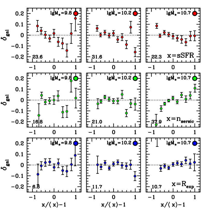
According to Figure 2, the answer depends on the property in question. As detailed in §2, all results in this section are restricted to pure central galaxies that lie on the SFMS. Each row shows results for a different galaxy property. The bottom row shows results when binning galaxies by , the scale radius of the exponential fit to each galaxy’s light profile. The middle row shows results for , the best-fit Sersic index to the galaxy light profile. The top row shows results when binning galaxies by sSFR. The columns show bins in stellar mass. From left to right, the bins are , , . Wide bins are necessary to increase the statistical power of the samples. In each panel, the -axis is the galaxy property relative to the mean. Due to the width of the bin, the mean of a galaxy property can evolve significantly from the low-mass end of the bin to the high-mass end. To prevent biases from this evolution, the mean galaxy property is first calculated in 0.1-dex sub-bins of , and the each galaxy’s properties are with respect to the mean in the sub-bin. Errors represent statistical errors in the mean.
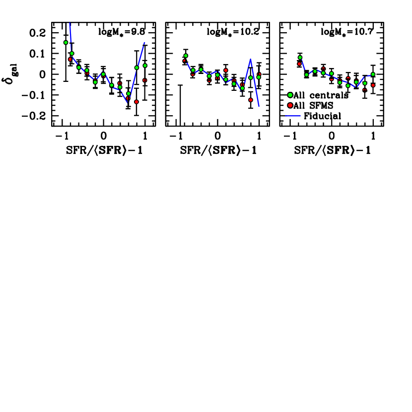
The top row shows results when binning galaxies by sSFR. In each panel, there is a clear correlation between and such that galaxies that are stronger than average star-formers live in lower densities, while below-average star-formers live in higher densities. The slope of this correlation is monotonically shallower with higher , but in each panel there is a statically significant correlation: using a statistic to test the consistency of each panel’s result with a straight line yields values of 23.6, 31.6, and 22.3 for each panel from left to right, respectively, for 10 data points in each panel. The error bars are smaller for higher bins due to the increased volume available for higher-mass samples. We will discuss this correlation in the context of dark matter halo growth in the following subsection.
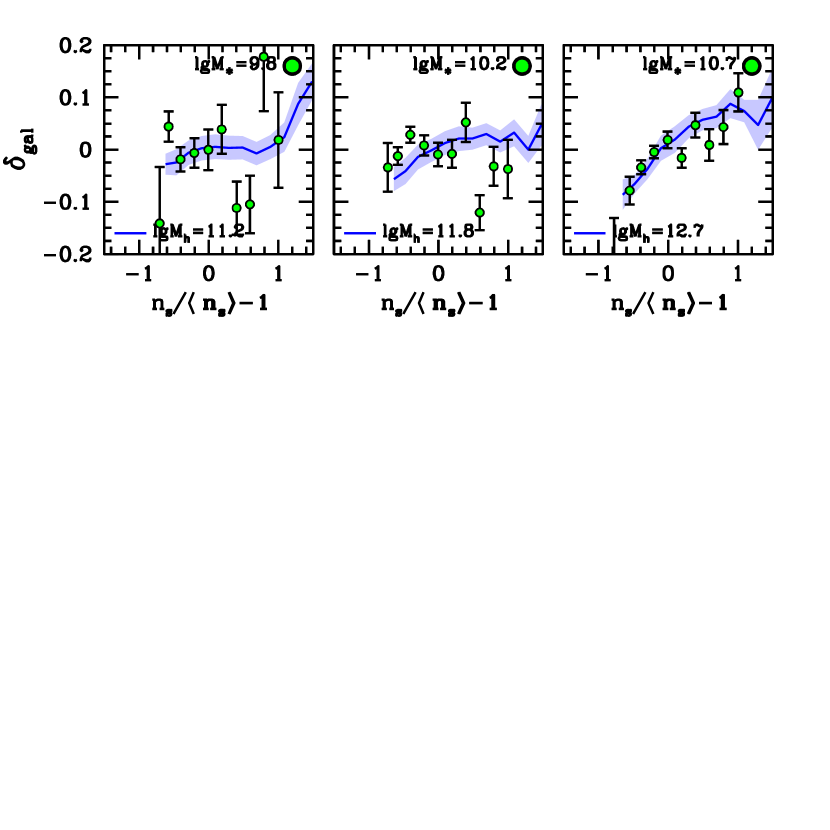
The middle row shows results when binning galaxies by . There is no clear correlation between and for , but at high masses a statistically significant correlation exists. In the far-right panel, galaxies with higher —i.e., galaxies with more elliptical and less disky morphology—live in slightly higher than average density environments. Galaxies that are more disk-dominated, however, live in significantly lower densities than average. The test described above yields values of 16.8, 21.0, and 37.9 for the panels from left to right, respectively. The of 21.0 for the middle panel is mostly driven by the datum at , without which the is 8.0. The large for the high mass bin is distributed more evenly in the data. Removing the far left datum, which has , reduces the to 32.
The bottom panel shows results for . In all panels, there is no clear dependence of on . The test yields values, from left to right, of 6.8, 11.7, and 10.7. There is a slight positive slope in the high-mass bin. A line with a slope of 0.05 yields a with respect to a straight line, but a straight line fit is statistically reasonable given 10 data points. We will discuss these results in the context of halo angular momentum in subsequent subsections.
3.2 Does Halo Growth Rate Correlate with Galaxy Growth Rate?
Using the method described in §2.3, we match halo growth rate to galaxy sSFR. In this scenario, the fastest growing halos have the highest star formation rates, while the slowest growing halos (or negatively-growing halos) have the lowest sSFR values. Because there is a correlation between halo growth rate and halo environment, this will impart a strong correlation between and in the. It is important to note the results of Papers I and II, which imply that quenching is a stochastic process with respect to halo growth rate, especially for halos with . Thus, star-forming halos are likely not a ‘special subset’ of dark matter halos, and we can draw from the full population of halos to make predictions.
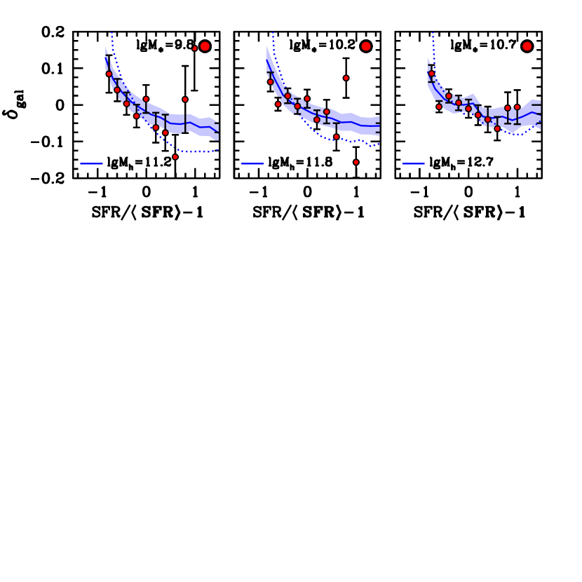
Figure 3 compares two theoretical models to the data presented in the top row of Figure 2. The dotted curves show one model in which is mapped onto sSFR assuming no scatter between the two quantities. The solid curves are the results of a model in which the scatter between these two quantities is 0.25 dex. Both models yield results that are qualitatively in good agreement with the data: the models predict and inverse correlation between star formation rate and , with a slope that monotonically decreases with increases . The slope of the correlation predicted in the no-scatter model is too steep relative to the data, especially for the slowest-growing halos. The model that incorporates scatter, however, is in excellent agreement with the data. The value of 0.25 dex was obtained by finding the scatter that yielded the lowest when comparing the model to the data, with a value of 28 for 30 data points. This model yields a of 21 with respect to a model with no correlation (but has the same errors as the simulation). A scatter of 0.25 dex in sSFR is approaching the overall scatter of in the SFMS of 0.28 dex, but even with this amount of scatter at fixed , the model still creates a significant correlation between sSFR and . These values imply a correlation coefficient of between and sSFR.
3.3 Does merger activity correlate with galaxy light profile?
Figure 4 shows the - relation first presented in Figure 2, but now with a comparison to the model in which is abundance matched onto at fixed . Error bars are calculated by jackknife sampling of the simulation volume into 8 sub-volumes. The slightly larger error bars in this comparison, relative to those seen in Figure 3 and what we will see in Figure 6 are due to the smaller box size of this simulation.
In all three panels, the model shows no evidence of a correlation between and , and thus yields no correlation between and . In our fiducial model, we incorporate 0.2 dex of scatter in at fixed . This value is consistent with recent measurements (e.g., Reddick et al. 2013; Zu & Mandelbaum 2015; Tinker et al. 2017). Physically, the amount of merging a galaxy has over its lifetime may contribute to this scatter, but this is not reflected in our fiducial implementation. Thus, we have run an additional model in which there is no scatter at . The results are unchanged, verifying that our fiducial model is not affected by uncorrelated scatter.
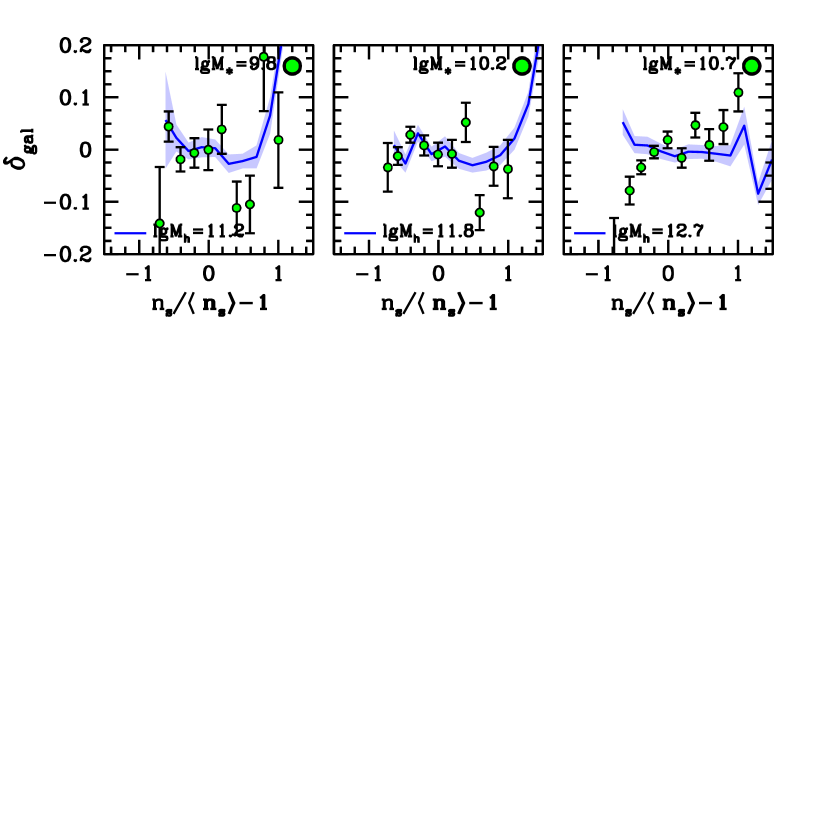
The parameter need not be correlated only to , but it is difficult to find another halo parameter that could match the signal measured in Figure 4. This is due to the fact that assembly bias created by most halo parameters is maximal at low halo masses— . These parameters include , , or short-term halo growth, . However, halo spin parameter yields a rather different assembly bias signal than these other parameters (see, e.g, Gao & White 2007). For , the assembly bias signal actually gets larger with higher halo mass, and goes away completely at . Figure 5 shows the comparison between measurements and an abundance matching model which maps onto , with no scatter, at fixed . This comparison is quite favorable, matching the slope of the observed correlation at and showing little-to-no correlation in the lower mass bins. For comparison, in the right-hand panel, we also show a model with 0.16 dex of scatter between and . The slope of the correlation is notably shallower, although it is difficult to distinguish between them given the noise in the data. Formally, when combining the jackknife errors from the simulation to the errors in the SDSS centrals, the minimum is achieved with a scatter of 0.11 dex, with a range of . These values add the errors in the model and the errors in the data in quadrature.
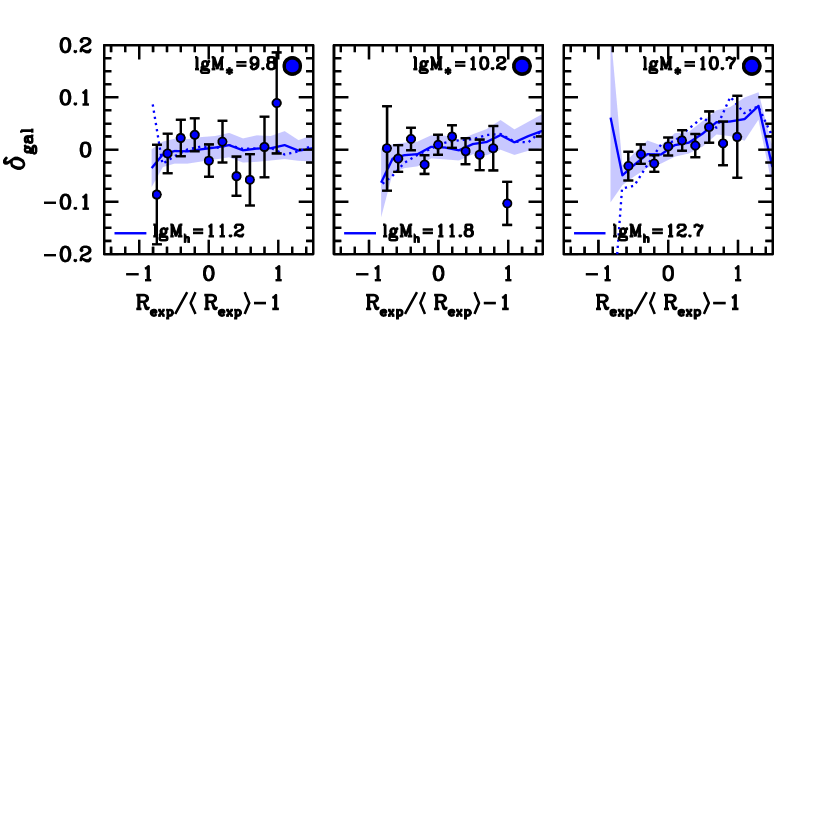
3.4 Does Halo Angular Momentum Correlate with Galaxy Disk Size?
As already shown in the previous subsection, the assembly bias signal created by halo spin has minimal amplitude at , but becomes measurable for galaxies that live in higher mass halos. For , there is a clear correlation with environment at , and this correlation is consistent with a model in which is strongly correlated with . For , the observational situation is less clear. In our high-mass galaxy bin, there is a measurable slope in the - data, but the statistical significance is low, given that a straight-lin fit yields a of 10.7 for 10 data points.
Figure 6 compares these data to an abundance matching model that maps onto at fixed . As described above, this model assumes a lognormal distribution of with a scatter of 0.2 dex. As expected from Figure 5, the assembly bias signal of this model is minimal in the first two stellar mass bins. But in the highest bin, the model yields a measurable signal. The dotted curves in Figure 6 show the model with no scatter between and . The correlated between and created in this model is stronger than that seen in the data. The solid curves show a model with 0.17 dex in scatter in at fixed . This model yields a slightly better fit to the data than a model with no correlation. To put the comparison on equal footing, we use the errors in the model to calculate a new for the no-correlation model. This reduces the from 10.7 to 3.9 for this model. The model with 0.17 of scatter in the relation yields a of 1.4.
4 Discussion
Papers I and II of this series demonstrated that large-scale environment—and, by extension, halo growth history—plays a limited impact on whether a central galaxy is quenched. In this paper we have restricted our analysis to central galaxies that lie on the star-forming sequence, allowing us to examine properties that are unique to such galaxies; the star-formation rates, disk sizes, and light profiles. As with Paper I and II, previous investigations have focused on how assembly bias might impact either galaxy bimodality (see, e.g., Lacerna et al. 2014; Lin et al. 2016) or the full galaxy population (e.g., Tinker et al. 2008; Zentner et al. 2016). This is the first study to look at secondary properties within the set of star-forming galaxies.
4.1 Assembly bias and star formation rates
Our results indicate that, at fixed stellar mass, central galaxies on the SFMS have higher star formation rates in lower density environments. These data are consistent with a model in which sSFR is correlated with near-term halo growth rate. This is a detection of assembly bias within this class of galaxies. It demonstrates consistency between the assumptions of the abundance matching model—namely, that galaxy growth should be correlated with halo growth—and the properties of observed star-forming galaxies.
Extrapolated to high redshift, this result implies that the total stellar mass of the galaxy is related to the formation history of its host halo. Using redshift-dependent abundance matching, Behroozi et al. (2013b) calculated the efficiency of converting accreted baryons into stars as a function of both time and halo mass. For halos less massive than at , this efficiency is lower at higher redshift than it is today. Thus, halos that form early accrete most of their baryons when this conversion efficiency is low, and will form galaxies that are less massive than late-forming halos of the same mass that accrete most of their mass at when efficiencies are higher. Tinker (2017) demonstrated that this is a source of scatter in the stellar-to-halo mass relation.
This is, however, the opposite of the assembly bias described in Lim et al. (2016) and measured in the GAMA survey by Tojeiro et al. (2016). In Lim et al. (2016), the ratio of is a proxy for halo formation time, with halos with higher forming earlier. This effect is also seen in hydrodynamic simulations (Matthee et al. 2017). In these models, halos that form early accrete significant amounts of gas early, and this gas therefor has a longer timescale over which to form stars. These two scenarios make mutually exclusive predictions for the halos around these galaxies. At fixed halo mass, the abundance matching model predicts that later-forming halos have larger galaxies, while in the SAMs and hydro simulations, early-forming halos have larger galaxies. Thus, at fixed central galaxy stellar mass, abundance matching predicts that halo mass will increase as you go from sSFR/sSFR to . The other models will predict the opposite trend. Galaxy-galaxy lensing or satellite kinematics may be able to provide discriminating information.
4.2 The role of spin in galaxy formation
The correlation between other SFMS galaxy parameters— and —is less clear. At galaxy masses , the data show no correlation between large-scale environment and these properties. However, for our high-mass galaxy bin, , the data show a positive correlation between both parameters and . For , the correlation is highly significant, while for , a model with no correlation is still a satisfactory description of the data. These trends in the data are consistent with a model in which both parameters are positively correlated correlated with halo angular momentum, parameterized by the the spin, . Halo properties that are tightly linked with halo growth history, , , and , show strong assembly bias at low halo masses, at . This is consistent with how the observed correlation between SFR and changes with . However, halo spin shows a distinctly different relationship with large-scale environment at fixed mass. Bett et al. (2007) show that spin is uncorrelated with large-scale environment at , but at higher halo masses, halos with higher spin exhibit stronger clustering. The only other halo property that shows this trend of stronger assembly bias at higher halo masses is the total number of subhalos within the parent halo (Croft et al. 2012; Mao et al. 2017).
The similarity between the assembly bias signals of and amount of substructure suggest that the two are correlated. In traditional tidal torque theory, angular momentum is imparted on a halo at early times, when structure is still linear, and is related to the distribution of matter in the initial density field (see, .e.g, Porciani et al. 2002). Alternatively, Vitvitska et al. (2002) proposed a model for the origin of halo spin through accretion of substructure. Major mergers spin up halos significantly, while angular momentum is also accumulated through lower-mass halo mergers.
However, if merging and spin are correlated, and through this correlation yield the same assembly bias signal, why does our merger model fail to produce a correlation between and ? Perhaps the smaller simulation volume, Mpc/, limits our ability to make a clear detection. Or it is possible that our chosen statistic, , is not optimal to detect the assembly bias signal. Galaxy mergers are quite different than halo accretion events, and given the steepness of the stellar-to-halo mass relation at low masses, it is possible for a halo to have a number of accretion events without building up much stellar mass through such events (see, e.g., Maller 2008). Or, as pointed out by Mao et al. (2017), even though the two properties are correlated, it is still possible that the scatter in this correlation eliminates any assembly bias signal in one of the two properties.
Rodriguez-Gomez et al. (2017) investigated the correlation between galaxy morphology, spin, and merger activity in the Illustris simulation. In their results, spin does correlate with morphology, but only for lower-mass galaxies. Spin may influence galaxy properties at low mass in our SDSS samples as well, but since does not yield and assembly bias in the host halos of these galaxies, there is no observational signature of such a correlation. The statistic probed in Rodriguez-Gomez et al. (2017) was the fraction of total kinetic energy in the galaxy contributed by rotational motion, which is not possible to measure directly in the full group catalog.
We also note that the results of Paper I appear similar to those of and ; at low galaxy masses, there is no correlation between the quenched fraction of central galaxies and . However, at higher stellar masses, there is indeed a small but non-zero slope in the correlation such that central galaxies in higher density regions are more often quenched. This is consistent with the assembly bias yielded from a correlation with halo spin, but the implication would be that higher spin halos are more likely to be quenched. At first glance, this result would seem to challenge the traditional orthodoxy of galaxy formation within dark matter halos—namely, that high-spin halos would form rotationally supported galaxies. As noted by Vitvitska et al. (2002), however, if spin is indeed created by mergers, the merger activity may cause galaxy transformation. The merger scenario for galaxy quenching has come into question, as hydrodynamical simulations suggest that, without the presence of an active post-merger feedback mechanism, star-formation is likely to be restarted after the merger is complete (Pontzen et al. 2017). But mergers may still temporarily quench galaxies, or the induced quenching may be permanent for some small fraction of merger events.
Of course, we cannot rule out the possibility that the agreement between the halo spin abundance matching models and the data is simply coincidence. But the results here indicate that it further investigation of the secondary properties of passive galaxies—their velocity dispersions, size, and light profiles—may elucidate the processes that caused their transformation to the red sequence.
4.3 Emission-Line Galaxy samples as cosmological probes
The detection of assembly bias in star forming objects may have implications for the use of such objects as tracers of the dark matter density field. The emission line galaxy (ELG) has been situated as the cosmological workhorse for the next generation of galaxy redshift surveys. Data are already being taken on a cosmological sample in the eBOSS program (Dawson et al. 2015; see Raichoor et al. 2017 for details of the ELG selection). Assembly bias in ELG samples would alter both their large-scale bias and the shape of their clustering, relative to a model that assumes that halo mass is the only property that determines their occupation (Sunayama et al. 2016). This is unlikely to bias measurements of baryon acoustic oscillations, but may have an impact on efforts to use clustering as a probe of the growth rate, neutrino masses, and non-Guassianity. Given the high precision expected from the clustering measurements of ELG samples, further investigation of the possible impact of the type of assembly bias measured here is warranted.
Acknowledgements
The authors wish to thank Michael Blanton, Rita Tojeiro, and Risa Wechsler for many useful discussions. The authors thank Matthew Becker for providing the Chinchilla simulation used in this work. The Chinchilla simulation and related analysis were performed using computational resources at SLAC. We thank the SLAC computational team for their consistent support. JLT acknowledges support from National Science Foundation grant AST-1615997. AW was supported by a Caltech-Carnegie Fellowship, in part through the Moore Center for Theoretical Cosmology and Physics at Caltech, and by NASA through grant HST-GO-14734 from STScI.
Appendix A Abundance Matching for Star Formation Rate
First, we assume the SFMS is a lognormal. Thus, the cumulative rank at any location in the distribution can be expressed as
| (2) |
where is a normalized rank in the range and is defined as
| (3) |
and we assume is 0.3, independent of stellar mass. For the case of no intrinsic scatter between and SFR, the rank-ordered list of halos can be matched to SFR by inverting equation (2). To include intrinsic scatter, , we assume that the total scatter in SFMS is 0.3, and the value used in equation (3) is
| (4) |
Thus, after determining the SFR of each halo based on abundance matching, each halo receives an additional SFR drawn from a Gaussian distribution with zero mean and .
Appendix B Testing Different Samples of Central Star-Forming Galaxies
In Figure 7, we show measurements of the correlation between SFR and for different samples of star-forming galaxies. Our fiducial sample contains only star-forming galaxies likely to be on the SFMS. Thus we randomly remove galaxies with low star formation rates in order to preserve the lognormal distribution of SFR. Additionally, our fiducial sample contains only central galaxies indicated as ‘pure’ centrals by the group catalog. These are centrals with . Removing non-pure centrals only reduces the overall sample size by .
In FIgure 7 we compare our fiducial measurements to those for samples in which we relax the restrictions on the sample. The blue curve is the fiducial measurement from Figure 2. The green circles show measurements that include all central galaxies, not just pure centrals. The red circles show measurements for all star-forming galaxies down to a specific SFR of yr-1. In both of these tests, the results are fully consistent with the fiducial measurement.
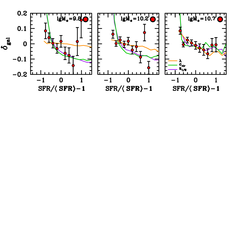
Appendix C Comparison of SFR Results to Different Halo Properties
Figure 8 compares the measurements of the SFR- correlation to abundance matching models that use halo properties other than as a proxy for star formation. Here we replace with , the redshift at which the halo reached half its present-day mass, the concentration parameter , and the halo spin parameter . For the first two halo properties, there is a correlation between , and (see, e.g., Wechsler et al. 2002). Thus, all of these halo properties yield similar correlations. We note, however, that the sign of the correlation is opposite to that of . In Figure 3, halos with the highest had the highest SFR. For and , halos with the lowest values of these properties have the highest star formation rates. Note that there is no scatter introduced in these comparisons.
As expected from Figure 5 and 6, the assembly bias signature created by a model that matches to SFR does not compare favorably to the data. Here, again, we assert an inverse relationship between spin and star formation rate, with no scatter.
For , We do find some dependence on the time baseline over which is calculated. The maximal assembly bias signal is found for calculated over a redshift baseline of . Smaller values of correspond to smaller assembly bias signals. At baselines larger than 0.8, the assembly bias signal is largely unchanged. We have not shown these results to preserve clarity in the plot, but the results for are comparable to those for .
References
- Abazajian et al. (2009) Abazajian K. N., et al., 2009, ApJS, 182, 543
- Behroozi et al. (2013a) Behroozi P. S., Wechsler R. H., Conroy C., 2013a, ApJ, 762, L31
- Behroozi et al. (2013b) Behroozi P. S., Wechsler R. H., Conroy C., 2013b, ApJ, 770, 57
- Behroozi et al. (2013) Behroozi P. S., Wechsler R. H., Wu H.-Y., 2013, ApJ, 762, 109
- Behroozi et al. (2013) Behroozi P. S., Wechsler R. H., Wu H.-Y., Busha M. T., Klypin A. A., Primack J. R., 2013, ApJ, 763, 18
- Bett et al. (2007) Bett P., Eke V., Frenk C. S., Jenkins A., Helly J., Navarro J., 2007, MNRAS, 376, 215
- Blanton et al. (2005) Blanton M. R., Lupton R. H., Schlegel D. J., Strauss M. A., Brinkmann J., Fukugita M., Loveday J., 2005, ApJ, 631, 208
- Blanton & Roweis (2007) Blanton M. R., Roweis S., 2007, AJ, 133, 734
- Blanton et al. (2005) Blanton M. R., Schlegel D. J., Strauss M. A., Brinkmann J., Finkbeiner D., Fukugita M., Gunn J. E., Hogg D. W., Ivezić Ž., Knapp G. R., Lupton R. H., Munn J. A., Schneider D. P., Tegmark M., Zehavi I., 2005, AJ, 129, 2562
- Brinchmann et al. (2004) Brinchmann J., Charlot S., White S. D. M., Tremonti C., Kauffmann G., Heckman T., Brinkmann J., 2004, MNRAS, 351, 1151
- Brooks & Christensen (2016) Brooks A., Christensen C., 2016, Galactic Bulges, 418, 317
- Bullock et al. (2001) Bullock J. S., Dekel A., Kolatt T. S., Kravtsov A. V., Klypin A. A., Porciani C., Primack J. R., 2001, ApJ, 555, 240
- Bundy et al. (2015) Bundy K., Bershady M. A., Law D. R., et al., 2015, ApJ, 798, 7
- Campbell et al. (2015) Campbell D., van den Bosch F. C., Hearin A., Padmanabhan N., Berlind A., Mo H. J., Tinker J., Yang X., 2015, MNRAS, 452, 444
- Chabrier (2003) Chabrier G., 2003, PASP, 115, 763
- Conroy & Wechsler (2009) Conroy C., Wechsler R. H., 2009, ApJ, 696, 620
- Croft et al. (2012) Croft R. A. C., Matteo T. D., Khandai N., Springel V., Jana A., Gardner J. P., 2012, MNRAS, 425, 2766
- Dalcanton et al. (1997) Dalcanton J. J., Spergel D. N., Summers F. J., 1997, ApJ, 482, 659
- Dawson et al. (2015) Dawson K. S., et al., 2015, ArXiv:1508.04473
- Dekel & Birnboim (2006) Dekel A., Birnboim Y., 2006, MNRAS, 368, 2
- Fakhouri & Ma (2009) Fakhouri O., Ma C.-P., 2009, MNRAS, 394, 1825
- Gao & White (2007) Gao L., White S. D. M., 2007, MNRAS, 377, L5
- Hahn et al. (2017) Hahn C., Tinker J. L., Wetzel A., 2017, ApJ, 841, 6
- Hearin & Watson (2013) Hearin A. P., Watson D. F., 2013, MNRAS, 435, 1313
- Hearin et al. (2015) Hearin A. P., Watson D. F., van den Bosch F. C., 2015, MNRAS, 452, 1958
- Hogg et al. (2003) Hogg D. W., Blanton M. R., Eisenstein D. J., Gunn J. E., Schlegel D. J., Zehavi I., Bahcall N. A., Brinkmann J., Csabai I., Schneider D. P., Weinberg D. H., York D. G., 2003, ApJ, 585, L5
- Kauffmann et al. (2013) Kauffmann G., Li C., Zhang W., Weinmann S., 2013, MNRAS, 430, 1447
- Kereš et al. (2009) Kereš D., Katz N., Fardal M., Davé R., Weinberg D. H., 2009, MNRAS, 395, 160
- Kereš et al. (2005) Kereš D., Katz N., Weinberg D. H., Davé R., 2005, MNRAS, 363, 2
- Lacerna et al. (2014) Lacerna I., Padilla N., Stasyszyn F., 2014, MNRAS, 443, 3107
- Lim et al. (2016) Lim S. H., Mo H. J., Wang H., Yang X., 2016, MNRAS, 455, 499
- Lin et al. (2016) Lin Y.-T., Mandelbaum R., Huang Y.-H., Huang H.-J., Dalal N., Diemer B., Jian H.-Y., Kravtsov A., 2016, ApJ, 819, 119
- Maller (2008) Maller A. H., 2008, in Funes J. G., Corsini E. M., eds, Astronomical Society of the Pacific Conference Series Vol. 396 of Astronomical Society of the Pacific Conference Series, Halo Mergers, Galaxy Mergers, and Why Hubble Type Depends on Mass. pp 251–+
- Mao et al. (2017) Mao Y.-Y., Zentner A. R., Wechsler R. H., 2017, ArXiv e-prints
- Matthee et al. (2017) Matthee J., Schaye J., Crain R. A., Schaller M., Bower R., Theuns T., 2017, MNRAS, 465, 2381
- Mo et al. (1998) Mo H. J., Mao S., White S. D. M., 1998, MNRAS, 295, 319
- Moster et al. (2013) Moster B. P., Naab T., White S. D. M., 2013, MNRAS, 428, 3121
- Noeske et al. (2007) Noeske K. G., Faber S. M., Weiner B. J., Koo D. C., Primack J. R., Dekel A., Papovich C., Conselice C. J., Le Floc’h E., Rieke G. H., Coil A. L., Lotz J. M., Somerville R. S., Bundy K., 2007, ApJ, 660, L47
- Pontzen et al. (2017) Pontzen A., Tremmel M., Roth N., Peiris H. V., Saintonge A., Volonteri M., Quinn T., Governato F., 2017, MNRAS, 465, 547
- Porciani et al. (2002) Porciani C., Dekel A., Hoffman Y., 2002, MNRAS, 332, 325
- Raichoor et al. (2017) Raichoor A., Comparat J., Delubac T., et al., 2017, MNRAS, submitted, ArXiv:1704.00338
- Reddick et al. (2013) Reddick R. M., Wechsler R. H., Tinker J. L., Behroozi P. S., 2013, ApJ, 771, 30
- Rodriguez-Gomez et al. (2017) Rodriguez-Gomez V., Sales L. V., Genel S., Pillepich A., Zjupa J., Nelson D., Griffen B., Torrey P., Snyder G. F., Vogelsberger M., Springel V., Ma C.-P., Hernquist L., 2017, MNRAS, 467, 3083
- Sunayama et al. (2016) Sunayama T., Hearin A. P., Padmanabhan N., Leauthaud A., 2016, MNRAS, 458, 1510
- Swanson et al. (2008) Swanson M. E. C., Tegmark M., Hamilton A. J. S., Hill J. C., 2008, MNRAS, 387, 1391
- Teklu et al. (2015) Teklu A. F., Remus R.-S., Dolag K., Beck A. M., Burkert A., Schmidt A. S., Schulze F., Steinborn L. K., 2015, ApJ, 812, 29
- Tinker et al. (2011) Tinker J., Wetzel A., Conroy C., 2011, MNRAS, submitted, ArXiv:1107.5046
- Tinker (2017) Tinker J. L., 2017, MNRAS, 467, 3533
- Tinker et al. (2017) Tinker J. L., Brownstein J. R., Guo H., Leauthaud A., Maraston C., Masters K., Montero-Dorta A. D., Thomas D., Tojeiro R., Weiner B., Zehavi I., Olmstead M. D., 2017, ApJ, 839, 121
- Tinker et al. (2008) Tinker J. L., Conroy C., Norberg P., Patiri S. G., Weinberg D. H., Warren M. S., 2008, ApJ, 686, 53
- Tojeiro et al. (2016) Tojeiro R., Eardley E., Peacock J. A., Norberg P., Alpaslan M., Driver S. P., Henriques B., Hopkins A. M., Kafle P. R., Robotham A. S. G., Thomas P., Tonini C., Wild V., 2016, submitted, ArXiv:1612.08595
- Vitvitska et al. (2002) Vitvitska M., Klypin A. A., Kravtsov A. V., Wechsler R. H., Primack J. R., Bullock J. S., 2002, ApJ, 581, 799
- Wechsler et al. (2002) Wechsler R. H., Bullock J. S., Primack J. R., Kravtsov A. V., Dekel A., 2002, ApJ, 568, 52
- Wechsler et al. (2006) Wechsler R. H., Zentner A. R., Bullock J. S., Kravtsov A. V., Allgood B., 2006, ApJ, 652, 71
- Wetzel et al. (2013) Wetzel A. R., Tinker J. L., Conroy C., van den Bosch F. C., 2013, MNRAS
- Wetzel & White (2010) Wetzel A. R., White M., 2010, MNRAS, 403, 1072
- White (2002) White M., 2002, ApJS, 143, 241
- Yang et al. (2005) Yang X., Mo H. J., van den Bosch F. C., Jing Y. P., 2005, MNRAS, 356, 1293
- Zavala et al. (2016) Zavala J., Frenk C. S., Bower R., Schaye J., Theuns T., Crain R. A., Trayford J. W., Schaller M., Furlong M., 2016, MNRAS, 460, 4466
- Zehavi et al. (2011) Zehavi I., Zheng Z., Weinberg D. H., Blanton M. R., Bahcall N. A., Berlind A. A., Brinkmann J., Frieman J. A., Gunn J. E., Lupton R. H., Nichol R. C., Percival W. J., Schneider D. P., Skibba R. A., Strauss M. A., Tegmark M., York D. G., 2011, ApJ, 736, 59
- Zentner et al. (2016) Zentner A. R., Hearin A., van den Bosch F. C., Lange J. U., Villarreal A., 2016, MNRAS, submitted, ArXiv:1606.07817
- Zu & Mandelbaum (2015) Zu Y., Mandelbaum R., 2015, MNRAS, 454, 1161