The chemical bond as an emergent phenomenon

Abstract

We first argue that the covalent bond and the various closed-shell interactions can be thought of as symmetry broken versions of one and the same interaction, viz., the multi-center bond. We use specially chosen molecular units to show that the symmetry breaking is controlled by density and electronegativity variation. We show that the bond order changes with bond deformation but in a step-like fashion, regions of near constancy separated by electronic localization transitions. These will often cause displacive transitions as well so that the bond strength, order, and length are established self-consistently. We further argue on the inherent relation of the covalent, closed-shell, and multi-center interactions with ionic and metallic bonding. All of these interactions can be viewed as distinct sectors on a phase diagram with density and electronegativity variation as control variables; the ionic and covalent/secondary sectors are associated with on-site and bond-order charge density wave respectively, the metallic sector with an electronic fluid. While displaying a contiguity at low densities, the metallic and ionic interactions represent distinct phases separated by discontinuous transitions at sufficiently high densities. Multi-center interactions emerge as a hybrid of the metallic and ionic bond that results from spatial coexistence of delocalized and localized electrons. In the present description, the issue of the stability of a compound is that of mutual miscibility of electronic fluids with distinct degrees of electron localization, supra-atomic ordering in complex inorganic compounds comes about naturally. The notions of electronic localization advanced hereby suggest a high throughput, automated procedure for screening candidate compounds and structures with regard to stability, without the need for computationally costly geometric optimization.

I Motivation

Chemical bonding is traditionally discussed in terms of the covalent, ionic, and metallic bond (doi:10.1021/ja02199a004), and weaker, closed-shell interactions such as secondary, donor-acceptor, hydrogen, and van der Waals. (Pyykko; Alcock1972) The distinction between these canonical bond types is not always clear-cut. For instance, a directional, multi-center (PapoianHoffmann2000) bond holding together identical atoms has an inherent ionic feature: In a three-center, linear $pp\sigma$ bond, (doi:10.1021/ja00884a026; pimentel:446) the central atom contributes only a half orbital to each of the individual $pp\sigma$ bonds. (MusherAngew1969) The terminal atoms, on the other hand, each contribute one full orbital, implying a non-uniform charge distribution over the bond. At the same time, the three-center $pp\sigma$ bond can be thought of as a limiting case of the metallic bond, since the appropriate electron count for an infinite chain corresponds to a half-filled band. (PapoianHoffmann2000) This identification is consistent with the metallic luster of compounds in which covalent and secondary bonds are comparable in length. (Alcock1972). In solid-state contexts, interplay between ionic and covalent interactions is often discussed using the van Arkel-Ketelaar triangle for binary compounds; (doi:10.1021/ed012p53; vanArkel; Ketelaar; Burdett1995) or revealed, for instance, in the taxonomies of classical valence compounds and Zintl phases. (GMiller1996; C5DT04140F). Contiguity between the metallic and ionic extremes is exemplified by metal-ammonia solutions, (SWmayo) whose electric conductance ranges between largely electronic and ionic, depending on the concentration of the metal.

Despite their distinct phenomenologies, canonical types of bonding are not always easy to distinguish on formal grounds, the case of the metallic bond being particularly subtle. Indeed, cohesive interactions in periodic solids are usually discussed either in terms of molecular orbitals (MO) or in terms of plane-wave, Bloch electronic states. (ABW) The two approaches are not equivalent: The majority of aperiodic condensed phases, such as liquids, frozen glasses, or amorphous films, are expressly not Bloch solids. (Within the Born-Oppenheimer approximation, liquids are solids as far as the electrons are concerned.) Yet the Bloch and MO approaches are often perceived as equivalent. In fact, there have been calls to do away with the concept of the metallic bond altogether, by including it under the broader rubric of covalent interactions. (AllenBurdett) Electron delocalization in aperiodic solids is of much subtler nature than in crystals; (AndersonLoc; Mott1993) one no longer speaks of allowed energy bands but, instead, of mobility bands. The latter are defined in a relatively narrow sense that individual molecular orbitals (MOs) extend further than the mean-free path of a charge carrier, a notion that harks back to the original motivation for introducing the metallic bond via the mobility of the electrons. (doi:10.1021/ja02199a004) The most important feature of the metallic bond is that the electrons do indeed comprise a fluid; an arbitrarily weak field results in a particle flow. No such flow can take place in insulators, where the electrons are fully localized.

In its ideal form—even if unachievable in actual compounds—the metallic bond is isotropic, not directional. This may directly reveal itself in the material’s being close-packed and/or malleable. Metallic substances tend to be poor glass-formers and decrease in volume upon crystallization, as perfect hard spheres would. In contrast, bond directionality characteristic of covalent interaction may even lead to expansion during freezing, as in water, silicon, or germanium. From the MO viewpoint, metals are special in that they possess a bulk density of (formally non-bonding) states that can be easily occupied at arbitrarily low temperatures. In contrast, the canonical covalent bond is defined most unambiguously as being due to filled states. From a thermodynamics vantage point, metallic and covalent interactions can be thought of as distinct since the metallic and insulating phases are separated by a phase transition. (Mott1993) The latter viewpoint will prove most instructive in the present context, the pertinent order parameter having to do with the degree of localization of the electronic liquid.

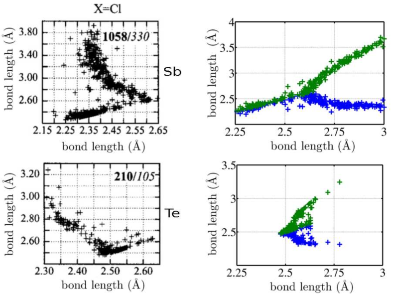
Figure 1: Left: The lengths of the two bonds in three-center bonding configurations compiled by Landrum and Hoffman. (LandrumHoffmann1998) Right: The Landrum-Hoffmann data replotted to show the two bond lengths as functions of the trimer length per bond.

The lack of clear dichotomies between canonically distinct chemical interactions is brought home by a systematic study by Landrum and Hoffmann,(LandrumHoffmann1998) who have screened thousands of compounds in the Oxford Structural Database for near linear trimeric motifs XQX, where Q stands for Sb or Te and X for F, Cl, Br, or I. Select parametric plots of the lengths $b_{1}$ and $b_{2}$ of the two individual bonds, from Ref.(LandrumHoffmann1998), are reproduced here on the l.h.s. of Fig. 1. The three-center bond in Fig. 1 is directional and exhibits back-bonding.(LandrumHoffmann1998) Indeed, the negative slopes of the $b_{2}\neq b_{1}$ portions of the parametric curves on the l.h.s. of Fig. 1 suggest that when shortened, the weaker bond supplies electrons into the anti-bonding orbital of the stronger bond, resulting in weakening of the latter. The shorter bond in the $b_{2}\neq b_{1}$ portions can be short enough to be considered covalent, while the longer, weaker bond varies in strength from what one expects for a relatively strong, directional secondary bond to a very weak van der Waals interaction, which is essentially non-directional. In the symmetric region, $b_{1}\approx b_{2}$, the bond strength can approach that of the covalent bond, for sufficiently small $b_{1,2}$. Thus empirical data suggest that the covalent, secondary, and three-center bonds form a true continuum of interactions. Despite some scatter in the data, one notices a great deal of universality in the $b_{1}$ vs. $b_{2}$ relation. While the synergic relation between complementary covalent and secondary bonds is expected based on straightforward molecular orbital considerations,(LandrumHoffmann1998) as just discussed, its apparent near universality is less obvious. This near universality suggests a law of corresponding states may apply.

Laws of corresponding states, such as the familiar van der Waals equation of state,(LLstat) often arise on a systematic basis in the context of critical points. If rescaled in terms of the critical temperature, pressure, and density, equations of state for chemically distinct substances will look identical near the critical point so long as those substances belong in the same universality class, (Goldenfeld) as defined by the symmetry and range of the interaction; the detailed form of interaction becomes immaterial because the molecular lengthscale is much shorter than the correlation length. In those common situations when a critical point is a limiting case of a set of discontinuous transitions—as is the case for the liquid-to-vapor transition, for instance—laws of corresponding states are still expected to hold approximately not too far from the critical point. When it holds, a law of corresponding states offers a systematic way to reduce the complexity of the problem by allowing one to use the simplest possible model from the universality class in question.

A revealing way to view the Landrum-Hoffmann data is to graph the two bond lengths as functions of the overall trimer length per bond $(b_{1}+b_{2})/2$, see the r.h.s. of Fig. 1. The graphs explicitly show an apparent symmetry breaking that takes place as the system expands from a high density state, in which $b_{1}\approx b_{2}$, to a state where the central atom chooses to make a strong bond with a specific neighbor, while settling on a weaker interaction with the other neighbor. The antimony and tellurium cases are distinct in that the broken-symmetry regime $b_{2}\neq b_{1}$ can coexist with the symmetric regime $b_{2}=b_{1}$ in the latter case, but not in the former. In the context of bulk phase transitions, lack of such coexistence implies the transition is continuous, a critical point. Incidentally, the density dependence of the bond lengths for the antimony compounds in Fig. 1 parallels that for the continuous transition between the rhombohedral and simple-cubic arsenic. (silas:174101) In contrast, a macroscopic phase coexistence implies the transition is discontinuous, common example being the liquid-to-solid transition. (LLstat; EhrenfestBook) Spatial coexistence of distinct types of bonding can be directly seen in the crystal of Bi₂Te₃, where multicenter, covalent, and secondary bonding patterns form extended layers, see Fig.2(a). This can be contrasted with As₂S₃, Fig. 2(b), a compound made of covalently bonded double layers that interact relatively weakly via secondary interactions; (ZLMicro1) each atom is surrounded by a Lewis octet.

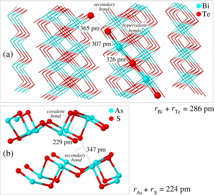
Figure 2: (a) Structure of Bi₂Te₃ illustrating coexistence of multicenter, covalent and secondary bonding. (b) Structure of As₂S₃ illustrating that the bonding is essentially covalent within the double layers. Sums of pertinent covalent radii are provided for the reader’s reference.

Here we argue that not only are the covalent bond and secondary interaction intimately related to each other and, in turn, to the multi-center bond, but that the covalent and secondary interaction can be thought of as originating from the multi-center bond as a result of a symmetry-breaking transition driven by a delicate interplay between steric repulsion and cohesive interaction. For sufficiently high electron count, the bond strength, order, and length establish self-consistently as a result of the transition. The ensuing differentiation in the bond length amounts to a breaking of spatial symmetry in the nuclear arrangement, as in Fig. 1. The transition could be either continuous or discontinuous. In the latter case, the discontinuity is weak and so a law of corresponding states still holds approximately.

We also observe two types of symmetry breaking of purely electronic origin, which occur even if the aforementioned differentiation in bond length does not take place or is artificially prevented by constraining the geometry. One type of transition occurs if one insists that the trial electronic wave-function be a single Slater determinant. As a result, the ground state as determined by solving the self-consistent Hartree-Fock (SCHF) equations could become degenerate. Each such solution represents a charge-density wave (gruner2009density; CanadellWhangbo1991) (CDW) formed as a result of electron-electron interactions. The true, quantum-mechanical ground state is unique; it is a superposition of those distinct “classical” solutions of the Hartree-Fock (HF) problem. (doi:10.1063/1.4832476) Still, the degeneracy is physically consequential and may signal a structural instability, if the overlap between those “classical” solutions is small. The other, subtler type of electronic transition takes place even as the molecular orbitals vary smoothly with geometry changes while the electronic density is redistributed among bonding orbitals and lone pairs. This type of transition manifests itself as a symmetry change of the effective wavefunctions of the bonding electrons, which we determine using the localized molecular orbital (RevModPhys.32.296; RevModPhys.35.457; doi:10.1063/1.1677859; PerkinsStewart1980; Levine09) (LMO) framework. (We will also find the LMOs to be particulary convenient in detecting the electronic symmetry breaking at the Hartree-Fock level.) Importantly we establish that away from narrow transition regions, the bond order and related quantities are found to be robust with respect to bond deformation, despite charge transfer accompanying nuclear motions.

We thus find that the order of a chemical bond is established as a result of transitions between states with distinct states of electron localization, often accompanied by displacive transitions of the nuclei. The bond order is apparently robust with respect to typical geometry fluctuations in a way that is analogous to how a phase of matter is stable while fluctuating within the corresponding free energy minimum. It may seem surprising, at a first glance, that finite systems such as molecules should exhibit phase transition-like phenomena that are normally associated with bulk, macroscopic phases. Yet a $D$-dimensional quantum system can be thought of a classical system in $(D+1)$ dimensions, the extent of the extra dimension proportional to the inverse temperature. (RevModPhys.69.315) In this sense, finding the ground state of even a small collection of atoms amounts to solving for a partition function of a classical system extending indefinitely along one spatial dimension; such systems do exhibit zero temperature fixed points. (Goldenfeld) Note the latter are associated with bound states. (Lfutile) Incidentally, a connection can be made with earlier work of Kais, Herschbach, and others, (KaisSerraACP; doi:10.1063/1.1637581) who have viewed ionization and dissociation as phase transitions with the nuclear charge being the control parameter.

We next extend the above results to bulk systems proper to argue that not only can distinct values of the bond order, but distinct types of chemical bond can be thought of distinct phases. The axes on the corresponding “phase diagram” of chemical interactions are density and electronegativity variation, respectively. The ionic and metallic bond can be viewed as fully distinct phases in that they are separated by one or more discontinuous phase transitions, above a certain threshold density. Such transitions were described by Kohn some 50 years ago. (PhysRevLett.19.789; PhysRevLett.19.439) Multi-center bonding is viewed as a coexistence, or hybrid, of the metallic and ionic bonding. The discontinuity of the transition stems from poor mutual miscibility of localized and delocalized electrons. Below the aforementioned threshold density, the metallic and ionic bond form a continuous spectrum of interactions. At sufficiently low values of mass density and electronegativity variation, the nuclear arrangement undergoes a symmetry-lowering displacive transition so that the multicenter bonding turns into a coexistence of covalent and secondary bonding, as it did for small molecular fragments. The venerable density-functional theory (PhysRev.136.B864) provides a formal foundation for and, at the same time, a convenient way to think about the phase diagram of chemical interactions: The covalent-secondary sector corresponds with the electrons forming a bond-order wave, while the ionic sector to an on-site charge density wave (CDW). (CanadellWhangbo1991) In the metallic sector, the itinerant electrons—despite being subject to the field due to the ionic cores that lowers the translational symmetry—could be thought of as a uniform liquid in the continuum limit.

In small molecules and bulk systems alike, the structural instabilities can be traced down to electronic instabilites arising from the formation of a bond-order charge density wave, the troughs and crests of the wave corresponding to weaker and stronger bonds in the eventual distorted structure. We implement this notion to show that an ambiguity in assigning of bonding electrons to effective two-center bonds signals structural instabilities and suggest a novel algoritm that can be used to speed up prediction of new compounds and structures.

In thinking of interactions as sectors on a phase diagram, we borrow the language from the renormalization group (RG) theory of phase transitions, (Goldenfeld; RevModPhys.70.653; RevModPhys.55.583) which operates on a space formed by coupling constants and, in general, by Hamiltonians. In the RG language, interactions and phases are interchangeable concepts. For instance, the paramagnetic and polarized states of a ferromagnet are viewed as (attractive) fixed points in a space formed by spin-spin couplings and the magnetic field. In the present framework, the role of the order parameter is played by the CDW type and strength; the description is coarse-grained, in full analogy with the RG framework.

The possibility of making a compound thus can be viewed as a question of coexistence of distinct types of charge density waves. For instance, while the Heusler and half-Heusler compounds are readily synthesized, (Graf20111) intermediate stoichiometries are not. In fact, the full- and half-Heusler phases exhibit poor mutual miscibility. (Romaka201345) Within the present formalism, those intermediate stoichiometries formally correspond to structures that interpolate between an insulating and metallic phase that are separated by a discontinuous transition and thus are automatically less stable than either of the two phases. One can likewise rationalize the variety of bonding preferences and structures in the semi-metallic region of the periodic table. For instance, the present notions provide a general understanding of why the structures of di-pnictogen tri-chalcogenides, such as those depicted in Fig. 2, show bonding ranging from essentially covalent in lighter elements to multi-center, hypervalent (PapoianHoffmann2000) interactions for heavier species. In addition, the latter compounds are organized, structure-wise, into stripes and ribbons despite the relatively uniform spatial distribution of the two constituent elements. Here we observe that the latter organization is analogous to lamellar ordering, which is common during phase coexistence. (SWmayo) Last but not least, the present results indicate that complications arising from those ambiguous bonding preferences are subject to universal relations in the form of laws of corresponding states. This justifies the use of semi-empirical, meanfield treatments exemplified by density-functional and tight-binding approximations, and even implicit-electron treatments such as the classical DFT, Landau-Ginzburg treatments of displacive transitions and multiferroic phenomena. (PhysRevLett.3.412; Dove1997)

The article is organized as follows: In Section II, we quantitatively analyse a substantial number of small molecular motifs to elucidate the mechanism of the symmetry breaking that leads to the emergence of the covalent and secondary bond from the multi-center bond, and its interplay with the ionic interaction. Section III discusses the electronic symmetry breaking underlying structural instabilities and the robustness of the concept of the bond order in molecular systems. In Section IV, we extend those arguments to the solid state context and build a phase diagram of chemical interactions. We summarize and discuss the present results in Section V.

II Interplay of covalent, secondary, multi-center, and ionic interactions: Small molecules

Figure 3: Lewis diagrams and the electronic configurations for the three-center $pp\sigma$ bond in the AsH₂-AsH_n-AsH₂ trimer, $n=2,1,0$ left to right. The two As-As bond lengths are assumed to be equal. The dashed lines for the $n=2$, 3/3 case indicate there are formally only 1.5 electrons per bond.

To investigate spatial symmetry breaking in small molecules, we analyse a number of $pp\sigma$ bonded trimeric units suitably passivated by hydrogens to achieve a desired number of electrons in the $pp\sigma$ bond. We begin from the AsH₂-AsH_n-AsH₂ trimer, $n=0,1,2$. According to the Lewis diagram in Fig. 3, this formally corresponds to a three-center bond that contains 5, 4, and 3 electrons, respectively, assuming each arsenic carries a lone pair. Our main focus is on the $n=1$ case, AsH₂-AsH₁-AsH₂, which corresponds to the classic 3-center/4-electron bond and, at the same time, obeys the Lewis octet rule. Consistent with the latter notion, it is the only molecule of the three that happens to be stable; the 3 and 5-electron molecules dissociate into a (passivated) dimer and monomer. The two As-As bond lengths, $b_{1}$ and $b_{2}$ respectively, are equal in the ground state of the 3/4 molecule.

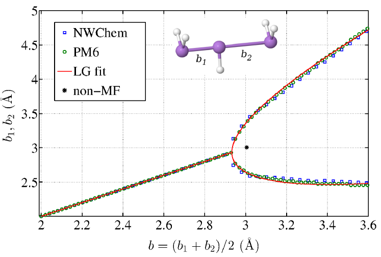
Figure 4: The equilibrium As-As bond lengths for the 3/4 case as functions of the overall trimer length, per bond, c.f. right top panel of Fig. 1. The energies are calculated using MOPAC and NWChem, see text. The arsenic atoms are constrained to lie on a straight line, while the As-H bonds lie in planes perpendicular to that line. The As-H bonds are fixed at length 1.5 Å ; mutual angle $90^{\circ}$ for the terminal bonds, see the inset. The molecule has two reflection planes. The asterisk denotes the location of the symmetry breaking corrected for zero-point vibrations of the molecule.

If stretched beyond a certain critical length, the molecule will dissociate and thus break the $b_{1}=b_{2}$ symmetry. This is shown in Fig. 4, where we plot $b_{1}$ and $b_{2}$ as functions of the overall trimer length per bond, $b\equiv(b_{1}+b_{2})/2$, which is externally imposed. The full potential energy surface of the molecule, as a function of the As-As bond lengths $b_{1}$ and $b_{2}$, is provided in the Supplementary Material. One set of curves in Fig. 4 corresponds to the semi-empirical approximation implemented in the package MOPAC with PM6 parametrization.(MOPAC2012; Stewart2007) MOPAC treats explicitly only the valence electrons, while using only a single, Slater-type basis function per atomic orbital and neglecting overlap between wave-functions on different centers during the self-consistent solution of the Hartree-Fock (HF) problem. (doi:10.1021/ja00457a004) (The corresponding matrix elements of the Hamiltonian are generally non-zero, of course.) The other set of curves is produced by a more accurate, ab initio approximation as implemented in the package NWChem (Valiev20101477) using the aug-cc-pVTZ-pp basis and a small, ten-electron effective core potential. MOPAC-optimized geometry compares well with the more accurate method, despite the relatively crude level of approximation. There are several motivations behind our use of MOPAC, to be discussed in due time.

The symmetry breaking transition in Fig. 4, c.f. Fig. 1, is continuous and apparently similar to classic examples of symmetry breaking such as the Curie point or the critical point in liquids. The transition can be formally described, at a meanfield level, using the Landau-Ginzburg expansion of the free energy (Goldenfeld) as a function of an order parameter reflecting the extent of symmetry breaking. In the present context, a convenient order parameter is the displacement $\Delta b\equiv(b_{1}-b_{2})/2$ of the central arsenic off the midpoint between the terminal arsenics. The corresponding Landau-Ginzburg expansion then reads:

$$F(\Delta b)=\frac{a_{2}}{2}(b_{c}-b)\,{(\Delta b)^{2}}+\frac{a_{4}}{4}{(\Delta b)^{4}},$$ (1)

where $b_{c}$ stands for the critical value of the trimer length $b$ per bond. The equilibrium value of the order parameter is determined by optimizing the “free energy” (1). The quantities $a_{2}$ and $a_{4}$ are system-dependent parameters. In the symmetry broken region, the displacement of the middle arsenic is thus given by a simple formula:

$$\Delta\tilde{b}=\pm(\tilde{b}-1)^{1/2},$$ (2)

where we have rescaled the control parameter by its critical value: $\tilde{b}\equiv b/b_{c}$, and the order parameter by an appropriate combination of the critical length $b_{c}$ and the expansion coefficients $a_{i}$: $\Delta\tilde{b}\equiv\Delta b/[a_{2}b_{c}/a_{4}]^{1/2}$. Eq. (2) is, of course, a system-independent, universal relation and thus constitutes a law of corresponding states. The best fit of the functional form (2) to the $b_{1}$ vs. $b_{2}$ dependences in Fig. 4 is shown as the solid red line in the same figure,

The apparently excellent fit of the bond lengths $b_{1}$ and $b_{2}$ to the meanfield expression (2) suggests correlations do not significantly affect the symmetry breaking. Still, the location of the bifurcation point in Fig. 4 is only a lower bound on the value of the critical length at which the actual symmetry breaking would occur. This is because already zero-point, let alone finite-temperature vibrations within either of the two individual minima on the symmetry-broken energy surface will allow the system to cross the barrier separating the minima, if the latter barrier is sufficiently low. Accordingly, one may assess the fluctuation-induced lowering of the critical point (Goldenfeld) semi-quantitatively, by requiring that those zero-point vibrations do not exceed the half-width of the barrier, see the graphical illustration in the Supplementary Material. The so estimated location of the critical point is shown by the asterisk in Fig. 4; it differs meaningfully from its meanfield value.

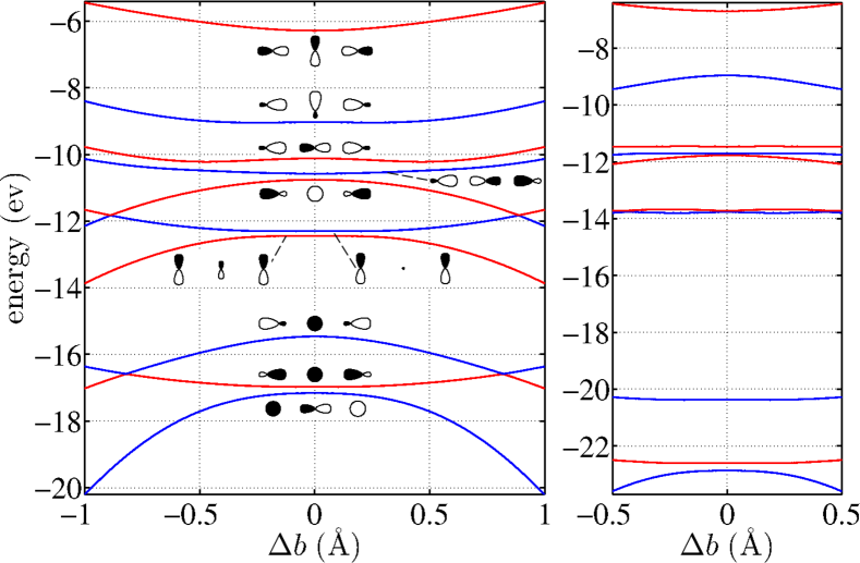
Figure 5: Walsh diagrams showing the energies of individual occupied MO as functions of the displacement $\Delta b$ of the central arsenic for the 3/4 trimer AsH₂-AsH-AsH₂. The distance $b_{1}+b_{2}$ between the terminal arsenics is 5.98 Å, which is just beyond the meanfield symmetry breaking point. The left and right panels show MOPAC PM6 and NWChem data, respectively; note the difference in the horizontal ranges.

In the aforementioned examples of the Curie point and the continuous vapor-to-liquid transition, the symmetric state is favored by entropic forces, while cohesive interactions favor the symmetry broken state. (L_AP) At the critical point, the two forces are in balance so that fluctuations of the order parameter incur zero cost. Likewise, we inquire what competing factors could drive the transition in Fig. 4. It should be immediately clear that in the $b\equiv(b_{1}+b_{2})/2\to\infty$ limit, the lowest energy state is asymetric. Informally speaking, a bond is better than no bond. In a more formal vein, symmetry lowering transitions in small molecules are often associated with Jahn-Teller instabilities. (ABW; Bersuker2006; Hargittai2008) (Such instability would have to be second order at least, in this case, because of symmetry.) In contrast, we observe in Fig. 5 that the HOMO is actually stabilized in the symmetric configuration. At the same time, the molecular terms behave all but generically near the symmetry breaking point. Fig. 5 displays the terms for a broad range of the displacement of the central arsenic as calculated using MOPAC PM6 and NWChem; the two calculations produce qualitatively similar results.

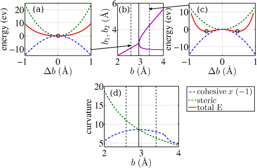
Figure 6: (a) The dependence of the cohesive contribution (green), repulsive contribution (blue) and the total energy (red) of the 3/4 trimer AsH₂-AsH-AsH₂ on the location of the middle arsenic, at a high density favoring the symmetric state. The circle indicates the location of the stable minima. (b) is the same as Fig. 4. (c) Same as (a), but at a low density favoring symmetry breaking. There are two equivalent minima now. Panel (d) displays the dependence of the absolute values of the curvatures of the repulsive and cohesive parts at $\Delta b=0$, on the trimer length. Vertical dashed lines indicate $b$ values associated with energy contours (a) and (c).

In search for alternative explanation, we note that by construction, MOPAC presents the full energy of the molecule as a sum of a cohesive and repulsive part: The cohesive part is evaluated by solving the HF problem using the valence electrons, as already mentioned. The steric part is parametrized to model the repulsion between the ionic cores. (We have verified that not much promotion of $3d$ electrons takes place at the densities in question, see the Supplementary Material.) In Fig. 6, we plot the cohesive and repulsive contributions, along with the total energy, in the symmetric and symmetry-broken regime. The cohesive part is increasingly stabilized for larger $\Delta b$. This is expected since the energy of the shorter bond depends sensitively on the bond length while the cohesive energy of the longer bond depends on the displacement already relatively weakly. The repulsive part is convex down and is minimized at $\Delta b=0$. At sufficiently high densities, the curvature of the repulsive term exceeds that of the cohesive part, thus stabilizing the symmetric, $b_{1}=b_{2}$ state. The opposite take place in a sufficiently long trimer, thus leading to a bistable potential corresponding to the emergence of two equivalent symmetry broken states.

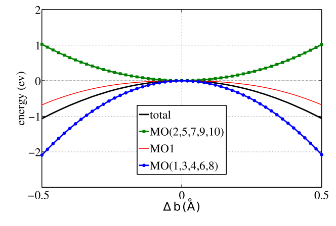
Figure 7: The solid black line shows the dependence of the MOPAC-inferred cohesive energy as a function of the location of the middle arsenic for the 3/4 trimer AsH₂-AsH-AsH₂. The sum of the MOPAC terms from Fig. 5 that stabilize and destabilize the symmetric state shown in green and blue respectively. The individual contribution of the lowest term is shown in red.

Fig. 7 provides a summary of the MOPAC-produced electronic terms from Fig. 5; it displays the total cohesive energy, the partial contributions of the terms that stabilize and destabilize the symmetric state, and, separately, the lowest-energy term from Fig. 5. The latter term clearly contributes most to the destabilization. We note that of the four terms favoring symmetry breaking, three terms, including the bottom one, stem from $sp$-mixing. Conversely, only one of the $sp$-mixed orbitals stabilizes the symmetric state. This suggests the symmetry breaking is driven to a large extent by $sp$-mixing, consistent with solid state precedents. (SeoHoffmann1999) The latter observation may seem in conflict with the expectation that the amount of $sp$-mixing should decrease with inter-atomic separation. This expectation is directly confirmed by the data in Figs. 8 and 9, where we show the contribution of the $s$ and $p$ atomic orbitals to the bond. We determine the latter contribution by a localization procedure, (RevModPhys.32.296; RevModPhys.35.457; doi:10.1063/1.1677859; NBO6) which is discussed in great detail in Section III. We observe that upon dilation of the 4-electron trimer, $sp$-mixing largely peters out by the time the spatial symmetry is broken. This process is even more dramatic for the electron-poor trimer $($AsH${}_{2})_{3}$, for which the bonding orbitals undergo a symmetry-breaking transition even as the trimer is still spatially symmetric. This, inherently electronic transition has to do with a transfer of electrons from the $pp\sigma$-bond to the lone pair on the central arsenic and will be discussed in Section III.

How does one reconcile the significance of $sp$-mixing for symmetry breaking, as apparent from Figs. 5 and 7, with its decrease at low densities, where the actual symmetry breaking occurs, Fig. 8? To resolve this apparent contradiction we note that although the destabilization of the symmetric state due to $sp$-mixing does decrease with interatomic separation for sufficiently long trimers, the stabilization due to steric repulsion diminishes even faster, see Fig. 6(d). This emphasizes a relatively subtle feature of the symmetry breaking: The cohesive and steric interactions both evolve similarly with density, at least at sufficiently low values of the latter. As the inter-nuclear distance decreases, electrons move toward the inter-atomic space because of the cumulative effects of Coulomb attraction to the involved nuclei; this stabilizes the cohesive component. At the same time, the steric repulsion also increases with density. The resulting bond enthalpy is therefore a modestly-sized quantity resulting from a delicate balance between two opposing, large quantities. We will observe a similar, but richer pattern in Section IV, in the context of density-driven coordination changes in solids.

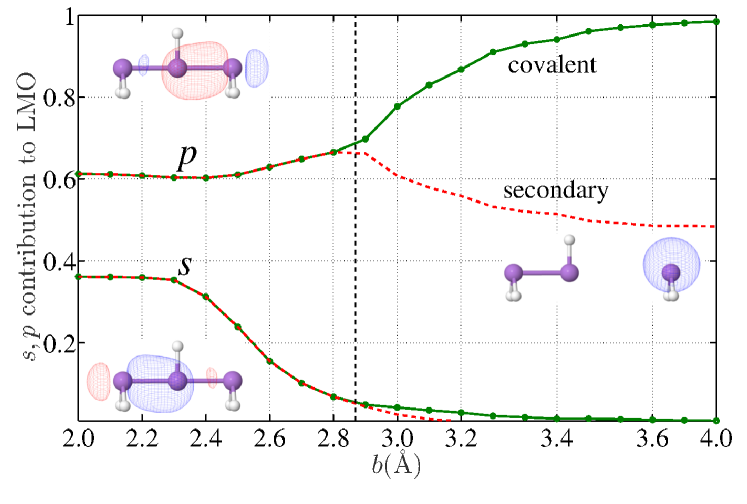
Figure 8: The $s$ and $p$ content of the localized molecular orbitals (LMOs), as functions of the trimer length per bond for the 3/4 trimer AsH₂-AsH-AsH₂. The localized molecular orbitals (LMOs) on the opposite sides of the symmetry breaking are exemplified in the insets.

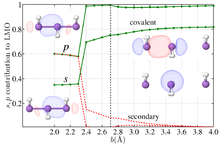
Figure 9: Same as Fig. 8, but for the 3/3 trimer AsH₂-AsH₂-AsH₂. The vertical dashed line indicates the length at which the spatial symmetry is broken. Note that the localized molecular orbitals exhibit a symmetry breaking while the molecule itself is still symmetric.

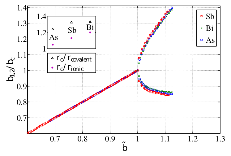
Figure 10: The dependences of the bond length for 3/4 trimers XH₂-XH-XH₂ (X = As, Sb, Bi), normalized by the respective critical length. The inset displays the ratio of the critical length in terms of the corresponding covalent and ionic radii for each element. The following values, in Å, for the covalent (ionic) radii for As, Sb, and Bi are adopted: 1.18 (1.39), 1.36 (1.59), (WBP72) 1.52 (CW80) (1.7 (WBP72)).

We next investigate whether our model trimeric units exhibit a universality of the type in Fig. 1, using the atom size as the control variable. Fig. 10 shows the “bifurcation” plots for three elements from group 15—As, Sb, and Bi—rescaled by the corresponding critical length. In the inset, we show the ratio of the latter length to the corresponding ionic and covalent radii for individual substances. We observe a fair deal of universality upon rescaling. At the same time, the critical length of the trimer, which is the characteristic length scale in the problem, is not strictly tied to common measures of the atomic size. In a systematic trend, the departure increases with the atomic mass. These conclusions are consistent with above findings on $sp$-mixing driving the symmetry breaking and the general notion that the amount of $sp$-mixing tends to decrease as one goes down the group in the periodic table. (PapoianHoffmann2000) In addition, the above trend is consonant with Clementi et al.’s (doi:10.1063/1.1712084) observation that the separation between the maximum charge-density radius of the outermost $d$ shell and valence $s$ and $p$ orbitals anti-correlates with the atomic number. In the present context, this implies that the effective size of the ionic core is greater for heavier atoms, relative to the extent of the frontier atomic orbitals. The resulting enhancement in steric repulsion thus serves to stabilize the symmetric configuration. Note that already rescaling both $b$ and $\Delta b$ with the critical length $b_{c}$ largely suffices in bringing all of the bifurcation graphs to a universal form; we will see shortly this simplification does not apply generally.

Similarly to the preceding discussion, we next study the effects of varying the electron content of the three center bond on the symmetry breaking. Specifically, we vary the number of passivating hydrogens on the AsH₂-AsH_n-AsH₂ trimer, as mentioned in the beginning of the Section. Similarly to Fig. 10, the bifurcation graphs follow a universal shape. In contrast with that situation, both variables $b$ and $\Delta b$ need to be rescaled, see the Supplementary Material. The critical lengths depend on the population of the $pp\sigma$ bond: $b_{c}=2.71$, $2.87$, and $2.63$ for three, four, and five electron bond, respectively. This is consistent with the view of the middle orbital of the $pp\sigma$ bond, Fig. 3, as mildly bonding. (PapoianHoffmann2000) We reiterate that the four-electron case satisfies the Lewis octet rule in the symmetric state. To avoid confusion we note that the electron count cannot be generally regarded as an independent control parameter but is determined self-consistently at given values of density and electronegativity variation, as is already clear from Figs. 8 and 9.

In discussing effects of electronegativity variation, we first recall that ionicity tends to suppress dimerization in extended one-dimensional systems. (PhysRevLett.49.1455; PhysRevLett.45.926) A similar effect can be seen at the extended-Hückel level for a hypothetical linear H${{}_{3}^{-}}$ molecule, Chapter 6.4 of Ref. ABW. We have checked that modifying the electronegativity variation along the trimer does not significantly affect the universality of the symmetry breaking, see Fig. 11 and Supplementary Material. There, we also demonstrate that the leading effect of introducing additional electronegativity variation is to shorten the bonds, that is, the critical length for a mixed trimer X-Y-X or Y-X-Y is usually less than the average of the critical lengths for the homoatomic trimers X₃ and Y₃. The effect is modestly stronger when the more electronegative element is placed at the terminal positions, consistent with the earlier notion that the three-center bond is already partially ionic because the terminal atoms contribute more electronic density than the central atom to the individual two-center bonds.

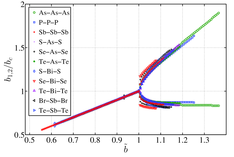
Figure 11: A number of bifurcation diagrams for pnictogen and chalcogen containing 3/4 trimers shown in reduced coordinates, as in Fig. 10. To maintain the 4 electron count, a chalcogen is passivated with one less hydrogen than a pnictogen.

The compilation of symmetry breakings for an extensive set of trimers, in Fig. 11, juxtaposes effects of varying the atom size, electronegativity, and valence. We again observe that every time continuous symmetry breaking takes place, a law of corresponding states holds already when one rescales all lengthscales by the critical length. If one were to rescale the bond-length difference $(b_{1}-b_{2})$, the universality would be even more pronounced. The rather extensive compilation in Fig. 11 shows that some of the trimers actually exhibit a discontinuous symmetry breaking, c.f. the bottom of Fig. 1. The energy surface for this more complicated situation now exhibits up to three minima, at $b=\text{const}$, see the Supplementary Material. In contrast with Fig. 1, the density range in which the symmetric and asymmetric molecule coexist is very narrow. Most likely such a discontinuity in a small molecule would be washed away by fluctuations, similarly to the lowering of the critical point in Fig. 4. On the other hand, in the solid state the discontinuity may will be significantly stabilized by the crystal field.

III Bond assignment as a result of electronic symmetry breaking

As discussed above, one may associate the spatial symmetry breaking in the 3/4 trimer with regard to the bond strength between neighboring arsenics with the spatial symmetry breaking $b_{2}\neq b_{1}$, at least for sufficiently large values of $|b_{2}-b_{1}|$. On the other hand, the relatively electron-poor 3/3 trimer exhibits an apparent change in bonding already in the symmetric $b_{1}=b_{2}$ configuration. To elucidate this type of electronic transition we consider two specific hydrogen-passivated trimers AsH₂-AsH-AsH₂ and AsH₂-AsH₂-AsH₂ while preventing the breaking of the $b_{1}\leftrightarrow b_{2}$ symmetry altogether. We shall impose an artificial constraint $b_{1}=b_{2}$ for all values of the trimer length. The hydrogens are constratined so that the molecule has two symmetry planes, one containing the 3-center bond and the other—call it plane $R$—perpendicular to the bond and containing the middle arsenic. Each MO thus must be either even or odd with respect to the reflection in plane $R$.

To quantify bonding in these symmetric trimers we use the localized molecular orbital (LMO) formalism. A pedagogical overview of the latter can be found in the Supplementary Material. Here, we only provide definitions and brief descriptions for several pertinent quantities. Originally inspired by symmetry adapted orbitals in relatively symmetric molecules, the localized molecular orbitals can be assigned for arbitrary geometries. One starts out with the molecular orbitals (MO) $\psi_{i}$

$$\psi_{i}=\sum_{A}\sum_{\lambda_{A}}\widetilde{C}_{\lambda_{A}i}\phi_{\lambda_{A}},$$ (3)

where $\phi_{\lambda_{A}}$ stands for an atomic orbital on atom $A$. Given a set of occupied MOs, one transforms to an alternative set of orthonormal orbitals $\chi_{j}$

$$\chi_{j}=\sum_{A}\sum_{\lambda_{A}}C_{\lambda_{A}j}\phi_{\lambda_{A}}$$ (4)

such that a certain quantity reflecting the self-repulsion within individual new orbitals is maximized.(RevModPhys.32.296; RevModPhys.35.457; doi:10.1063/1.1677859; PerkinsStewart1980) The quantities $\chi_{j}$, often called localized molecular orbitals (LMO), represent an attempt by an interpreter to partition (the already bound) electrons among orthonormal, maximally localized orbitals, each of which thus binds together the smallest number of atoms. The number of atoms inolved in the corresponding bond, or the bond center number $n_{j}$ is computed according to:

$$n_{j}\equiv\sum_{A}\left(\sum_{\lambda_{A}}C^{2}_{\lambda_{A}j}\right)^{2}.$$ (5)

The contribution the $j$-th LMO to a bond, as opposed to a lone pair for instance, is often called the “bonding contribution”

$$C^{\text{(bond)}}_{jj}\equiv\left\langle\chi_{j}|\widehat{P}|\chi_{j}\right\rangle=2\sum_{\lambda\mu}C_{\lambda j}C_{\mu j}P_{\lambda\mu},$$ (6)

where terms pertaining to the same atoms are excluded from the summation and $P_{\lambda\sigma}$ is the density matrix element

$$P_{\lambda\mu}\equiv 2\sum_{i}\widetilde{C}_{\lambda i}\widetilde{C}_{\mu i}.$$ (7)

The summation in Eq. (7) is exclusively over occupied MOs.

It will be useful to complement the LMO formalism, which is quite anthropocentric, with a more basic descriptor, viz., the number of electrons shared by atoms A and B, $B_{AB}$, often called the Wiberg index:(Armstrong73)

$$B_{AB}\equiv\sum_{\lambda_{A}\!,\,\lambda_{B}}P^{2}_{\lambda_{A}\lambda_{B}}.$$ (8)

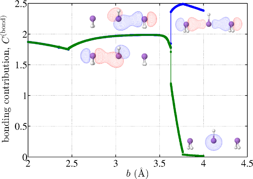
Figure 12: The bonding contribution of the LMOs as functions of the As-As bond length $b=b_{1}=b_{2}$, for the 3/4 case.

First off, we identify the localized molecular orbitals (LMOs) that are associated with the As-As-As subsystem, as opposed to the As-H bonds. There are two such LMOs. Their bond contributions, Eq. (6), are shown in Fig. 12 as functions of the trimer-length. In that same figure, we display the corresponding localized molecular orbitals themselves. The corresponding bond-center number, Eq. (5), and Wiberg bond index, Eq. (8), are shown in Figs. 13(a) and (b) respectively.

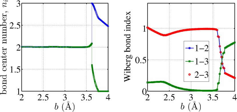
Figure 13: Displayed as functions of the As-As bond length $b=b_{1}=b_{2}$: (a), the bond center number for the LMOs from Fig. 12; (b), the Wiberg bond index. Note the latter is computed using the density matrix and does not rely on the localization procedure.

According to Figs. 12-13, the bond characteristics of the electron rich 3/4 trimer remain steady within a remarkably broad range of the inter-arsenic distance and are essentially the same as those in the ground state. The bond order eventually changes, at sufficiently low densities, and does so in an abrupt fashion, especially the bonding contribution. Figs. 12 and 13(a) indicate that the transition is truly discontinuous: Its precise location exhibits a hysteretic behavior and depends on the precise protocol such as the grid size for the quantity $b$ or the tolerance of the self-consistent Hartree-Fock (SCHF) procedure; the resulting ambiguity in $b$ is not large, however, a hundredth of an angstrom or so. The transition in the bond type is apparently accompanied by a symmetry change in the LMO. On the high density side, the LMOs are mirror images of each other and amount to the same bond contribution. Neither of these LMOs contributes to an irreducible representation of the molecule’s point group, only a linear combination does. On the low density side, in contrast, both LMOs are even functions with regard to the reflection in plane $R$. One LMO stretches over the three centers, consistent with its bond-center number and the bond contribution, while the other LMO is essentially a lone pair. The nearest-neighbor As-As bonds on the high-density side of the transition are unquestionably weak. The bond length at the transition—$b=3.628$ Å for the specific realization in Fig. 12—is about 50% longer than its equilibrium value and, in fact, is more appropriate for a closed-shell, secondary interaction. (ZLMicro1) Still, the interaction is not closed-shell since the formally antibonding orbital in the $pp\sigma$ bond is vacant, see graphical three-orbital representation in Supplementary Material. In any event, we have confirmed the symmetry breaking transition using a higher end approximation and alternative methods of conceptualizing molecular bonding, viz. the Natural Bond analysis (g09; NBO6) and the QTAIM theory, (doi:10.1021/jp983362q; MolinaMolina2001; BaderAIM; MacchiCDA) see the Supplementary Material. There, we also show that the molecular orbitals do eventually localize on the respective centers for sufficiently long trimers.

We next inquire whether the apparently abrupt change in the localized molecular orbitals is caused by an abrupt change in the canonical molecular orbitals, if any. Already a small molecule such as the AsH₂-AsH-AsH₂ has many molecular orbitals. Specifically, at the MOPAC level, each arsenic has nine orbitals per atom ($4s$, $p$, and $d$) and each hydrogen has one, that make substantial contributions to the MOs. Individually plotting a large number of molecular terms, as functions of density, is hardly illuminating. Instead, we make two scatter plots, Fig. 14(a) and (b), in which we show the change in the expansion coefficients $C$ and $\widetilde{C}$ from Eqs. (3) and (4) across the transition vs. their arithmetic average. The two sampling points are at $b=$ 3.61315 Å  and 3.61335 Å, respectively; this specific realization of the LMO-switching transition takes place for a slightly shorter trimer than in Fig. 12. According to the scatter plots, the changes in the MO expansion coefficients $\widetilde{C}$ are gradual; these changes are commensurate with the magnitude of the change in the bond length across the transition. In contrast, the coefficients $C$ of the LMO expansion change discontinuously. (A specific pair of LMOs were chosen for presentation in Fig. 14(b); others show the same trend.) One can thus rule out the possibility that the rapid change in the bond assignment is caused by a term-crossing, consistent with the results of direct inspection of the molecular terms, see the Supplmentary Material. Note that the Wiberg bond index from Fig. 13(b) changes noticeably, but continuously near the transition.

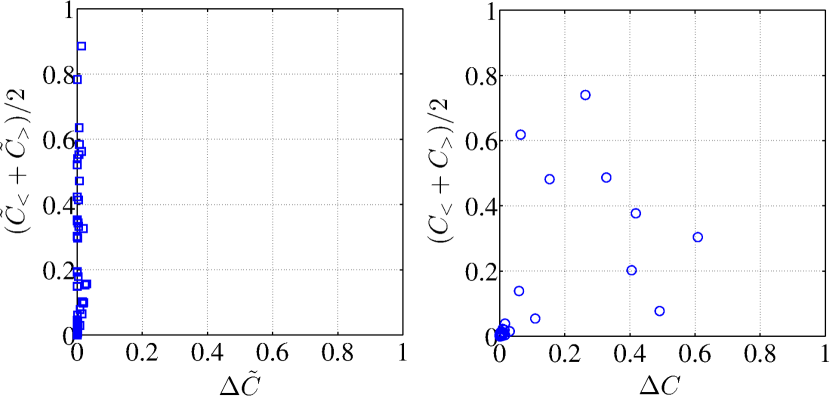
Figure 14: Scatter plots of the changes in the expansion coefficients of the MOs, (a), and LMOs, (b), upon the symmetry breaking transition in Fig. 12, vs. their average values.

The appearance of a discontinuous transition for the LMOs is not unexpected considering that the localization procedure, discussed in the Supplementary Material, is a non-linear problem. For the sake of concreteness, we will designate those transitions as “LMO-transitions,” to distinguish them from any transitions that happen already at the Hartree-Fock level, if any. We will see below that LMO-transitions occurring in the absence of an underlying transition at the HF level are an exception rather than the rule for larger systems.

The qualitative change in the LMO in Fig. 12 is consistent with the apparent destabilization of the MO corresponding to the $pp\sigma$ interaction, on the one hand, and stabilization of the MO corresponding to the lone pair on the middle arsenic, on the other hand. (The respective molecular terms are shown in Figs. S15 and S16 in the Supplementary Material.)

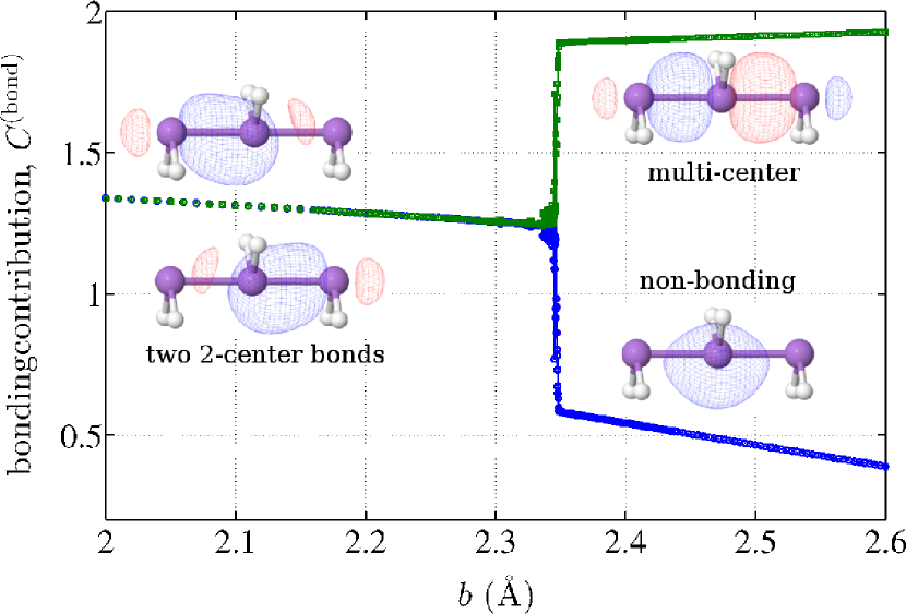
Figure 15: The bonding contribution of the LMOs as functions of the As-As bond length $b=b_{1}=b_{2}$, for the 3/3 molecule.

The above findings for the 3/4 trimer are consistent with our results for the 3/3 case AsH₂-AsH₂-AsH₂, which is of interest in its own right, see Fig. 15 and further discussion in the Supplementary Material. Because the $pp\sigma$ bond in the 3/3 trimer is one electron short, the molecule is only metastable in the symmetric geometry. Nevertheless, the molecule near its metastable minimum exhibits the bond lengths and LMO characteristics similar to those of the 3/4 trimer near its ground state. We thus observe that bringing the nuclei closer together induces sufficient amount of electron transfer out of the lone pair on the central arsenic so as to fill the $pp\sigma$ bond. This is witnessed by the formation of two two-center LMOs.

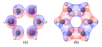
Figure 16: The localized molecular orbitals for the ground state of benzene.

In both 3/4 and 3/3 case, we observe that a stable (or metastable) three center bond is signaled by the presence of two two-center LMOs. One may formulate this notion in the form of the following, tentative rule: In a stable (or metastable) molecule, the bonding LMOs should be two-center and cover each nearest neighbor bond. Conversely, when the molecule is not fully covered by two-center LMOs, the molecule is subject to a structural instability. One may benefit from further illustration of these notions by considering the familiar example of the benzene molecule, see Fig. 16. Here we observe that of the 18 available valence electrons, 12 fill the $\sigma$ bonded network, leading to the formation of six two-center LMOs. The remaining six electrons amount to three non-two-center LMOs, which by itself would imply an instability. The instability is second order Jahn-Teller, and a finite-size analog of the Peierls instability. (Bersuker2006; ABW) The benzene molecule can be thought of as a superposition of the bonding situations on the opposite sides of the transition shown in Fig. 12. The amount of instability stemming from the non-bonding LMOs is however insufficient to break the spatial symmetry favored by the bonding LMOs, consistent with more sophisticated analyses; (ABW) benzene thus retains the six-fold, not three-fold symmetry in its ground state.

One may ask how extended an LMO could be. The most extended LMO we have succeeded in generating spans five centers, see the Supplementary Material. Consistent with the coverage rule above, such multi-center LMOs would appear at densities where the molecule is unstable.

The above ideas can be profitably applied to extended systems. Arguably the simplest example of such an extended system is a one-dimensional chain of equivalent orbitals, at half-filling. Already at the Hückel level, this model exhibits a rich behavior, if the bonds are allowed to deform, subject to a restoring force from the lattice. Using the creation (annihilation) operator $c_{n,s}^{\ddagger}$ ($c_{n,s}$) for an electron on site $n$ with spin $s$, the energy function can be written as:

$${\cal H}=\sum_{n}\sum_{s=\pm 1/2} \left[t(x_{n},x_{n+1})\,(c^{\dagger}_{n,s}c_{n+1,s}+c^{\dagger}_{n+1,s}c_{n,s})\right.$$

$$+ \left.(-1)^{n}\epsilon\,c_{n,s}^{\dagger}c_{n,s}\right]+{\cal H}_{\text{lattice}}(\{x_{n}\}),$$ (9)

where $t(x_{n},x_{n+1})$ is the hopping matrix element between sites $n$ and $n+1$, $(-1)^{n}\epsilon$ on-site energy, and ${\cal H}_{\text{lattice}}$ accounts for the elastic response of the lattice and the kinetic energy of the nuclei. In the lowest order expansion in bond deformation, $t(x_{n},x_{n+1})=t^{(0)}-\alpha(x_{n+1}-x_{n}-a)$, ${\cal H}_{\text{lattice}}=\sum_{n}k(x_{n+1}-x_{n}-a)^{2}/2+M\dot{x_{n}}^{2}/2$. In the absence of electronegativity variation, $\epsilon=0$, Eq. (9) gives the venerable Su-Schrieffer-Heeger Hamiltonian for trans-polyacetylene. (RevModPhys.60.781) A non-zero $\epsilon\neq 0$ was introduced by Rice and Mele to study heteropolar polymers. (PhysRevLett.49.1455; PhysRevLett.45.926)

At half-filling and in the absence of electronegativity variation, $\epsilon=0$, the system (9) held at uniform spacing between nearest sites is a metal. It is, however, Peierls-unstable with respect to dimerization, (Peierls; RevModPhys.60.781; ABW) $x_{n+1}-x_{n}=\pm(-1)^{n}\text{const}$, upon which it becomes an insulator. The gap is approximately proportional to the differential $\Delta t\equiv|t(x_{n},x_{n+1})-t(x_{n},x_{n-1})|$ in the hopping matrix element between the stronger and weaker bond; the gap is caused by scattering of the electrons near the wavelength corresponding to the unit cell of the distorted lattice, which now contains two lattice sites. In contrast, when the electronegativity variance is sufficiently large, the dimerization is suppressed while the material can be thought of as an ionic insulator; the gap is largely due to the work needed to transfer an electron from the more electronegative atom to its less electronegative counterpart, as is the case in sodium chloride for instance. As a rule of thumb, Peierls-dimerization will be suppressed when the electronegativity variation is comparable to $\Delta t$ the system would exhibit when $\epsilon=0$. (PhysRevLett.49.1455; PhysRevLett.45.926) For a chain of passivated arsenics, this is numerically close to 1-2 eV. Whether the chain from Eq. (9) becomes a Peierls or ionic insulator, it develops a charge density wave (CDW). (CanadellWhangbo1991) The presence of dimerization implies that the CDW has an off-site component, often called bond-order wave, while non-vanishing electronegativity variation implies the CDW has an on-site component. Thus at sufficiently low mass density and electronegativity, the one-dimensional chain from Eq. (9) will be a Peierls insulator.

To set the stage for the discussion of bonding in extended one-dimensional systems we note that the 3/4 trimer is unique in that it is the only case, in which the $n$-center, $(n+1)$ electron bond—corresponding to half-filling—is actually stable. This can be understood by using the two-center LMO coverage rule formulated above. By that rule, an $n$-center, $(n+1)$ electron bond is stable if there are enough electrons to fill $(n-1)$ LMOs, i.e., $n+1=2(n-1)$. (This is assuming there is no electron transfer from lone pairs or there are no additional sub-bands that could provide stability as in the benzene example above.) The equation is solved only by $n=3$, and so the multi-center bond becomes electron deficient for any molecule longer than $3$ centers. In the $n\to\infty$ limit, one obtains one electron per bond; a $($AsH${}_{2})_{n}$ chain will dimerize, if let go, (ZLMicro1) owing to the aforementioned Peierls instability. (Peierls; RevModPhys.60.781; ABW; ZLMicro1; ZLMicro2)

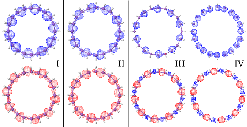
Figure 17: The localized molecular orbitals on the (AsH₂)₂₀ ring molecule shown for clarity as two sets of equivalent orbitals. The two colors correspond with the opposite signs. The ranges for each of the four regimes are shown in Fig. 18. The LMOs are shown for specific values of the bond length $b$: (I) $b=1.81$ Å, (II) $b=2.06$ Å, (III) $b=2.58$ Å, and (IV) $b=3.09$ Å. The specific value $b=2.58$ Å for regime III was chosen because at yet greater values of $b$, the ring becomes unstable with respect to dimerization.

We now consider a chain of passivated arsenic atoms with uniform spacing between nearest neighbors. To prevent symmetry-lowering due to open ends we consider a closed ring, viz., $($AsH${}_{2})_{20}$. The ring length 20 is sufficiently large so that the effects of $sp$-mixing due to the curvature of the $pp\sigma$ network are modest. The passivating hydrogens are fixed so that the molecule has $D_{20h}$ symmetry. Within the studied range of densities, we find four distinct bonding regimes which we label by roman numerals; representative LMOs are shown in Fig. 17.

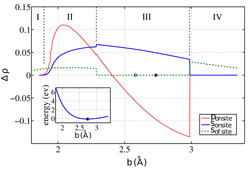
Figure 18: Dependence of the strength of the charge-density wave in the AsH₂)₂₀ ring on the bond length $b$. The $s$- and $p$-contributions to the on-site component are shown as solid lines, while the $s$-component of the off-site, bond order wave with the dashed line. Minimum energy configuration is marked with the asterisk; the bond length associated with the onset of dimerization, $b=2.58$ Å, with the circle.

Unlike in the trimer case, the LMO transitions for the 20-member ring are entirely due to symmetry breaking already at the level of the canonical molecular orbitals, as we demonstrate in Fig. 18. Visualizing changes in the molecular orbitals is difficult because of their large number. Here we take advantage of the fact that in the full density range in question, the electrons form a charge-density wave (CDW) commensurate with the periodicity of the chain. Indeed, consistent with the expectation that a 1D metal at half-filling is Peierls-unstable toward dimerization, the charge distribution exhibits a periodic pattern whose periodicity is twice that exhibited by the chain. Because the chain itself is fixed at uniform spacing between nearest neighbors, the symmetry breaking is entirely due to electron-electron repulsion. The symmetry lowering manifests itself via the formation of either on-site or off-site CDW, or both. To quantify the strength of the on-site charge density wave, we compute the variation in the diagonal entry of the density matrix:

$$\Delta\rho^{\text{(on)}}=\frac{1}{2}\sum(P_{\lambda_{2n+1},\lambda_{2n+1}}-P_{\lambda_{2n},\lambda_{2n}}),$$ (10)

where the summation is over a subset of orbitals of interest on any even-numbered and odd-numbered center, $2n$ and $(2n+1)$, respectively. The $s$ and $p$ contributions to the CDW strength are shown with the red and blue solid lines in Fig. 18. To quantify the off-site, bond-order wave, we limit ourselves to the $s$-orbitals, to avoid ambiguity stemming from arbitrary mutual signs of the respective contributions of the $p$ orbitals to the off-diagonal elements of the density matrix. Thus we compute the variation in the inter-atomic charge density of the $s$-electrons according to

$$\Delta\rho^{\text{(off)}}=\frac{1}{2}(P_{2n+1,2n}^{(s)}-P_{2n,2n-1}^{(s)}),$$ (11)

where the superscript $(s)$ signifies that only the $s$-orbital contribution to the density matrix is used. The quantity $\Delta\rho^{\text{(off)}}$ is shown in Fig. 18 with the dashed line.

The ground state of the system—subject to the aforementioned geometric constraints—falls in regime III, where only the on-site CDW is present. Of the three transitions between states with distinct CDW states, one is continuous (I $\leftrightarrow$ II) and the rest are discontinuous. Consistent with the preceding Section, the localized-molecular orbitals represent a sensitive indicator of charge redistribution: The CDW changes gradually between regimes I and II; the symmetry of the off-site CDW does not change, while the on-site component begins to gradually develop a pattern with a lower, ten-fold symmetry on the r.h.s. of the transition. In contrast, the LMOs show a pronounced symmetry breaking. On the lower density, larger $b$ side of the transition, the LMOs become chiral. To avoid any possible confusion we point out that the canonical MOs cannot and do not experience such a drastic symmetry breaking, given the geometric constraints. And so for every chiral MO, if any, there is a corresponding MO at the same energy but opposite handedness. Note that there appear to be a few, continuous “microtransitions” within regime II, however these do not modify the shapes of the LMOs qualitatively.

The presence of the charge density wave, Fig. 18, automatically implies that the Hartree-Fock ground state of the molecule is doubly degenerate, since rotation of the molecule by 360/20=18 degree results in a distinct yet equivalent electronic configuration. The presence of such a degeneracy is a consequence of our using a single-determinant wave-function. A better approximation for the actual ground state would be a superposition of those two distinct solutions. In physical terms, the presence of the degeneracy is a sign of the Peierls instability, as already mentioned. If equal spacing between nearest neighbors were not enforced, the molecule would readily convert into a ring made of ten equivalent dimers; there are two equivalent ways to dimerize. Incidentally, we note that unlike in the trimer case study in Section II, convergence of the self-consistent Hartree-Fock (SCHF) procedure for the 20-member ring was less robust. Decreasing the tolerance from the default value of $10^{-4}$ kcal/mol to a smaller value of $10^{-6}$ kcal/mol was helpful in finding lower energy solutions. Still, we cannot be certain that the solutions shown in Figs. 17 and 18 correspond to the lowest available Hartree-Fock energy.

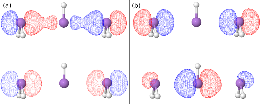
Figure S24: The bonding LMOs are shown for the AsH₂-AsH-AsH₂ for two values of the bond length, (a) $b=3.74$ Å  and (b) $b=3.76$ Å.

As in the trimer case, we observe that at sufficiently high densities, the LMOs are two-center and cover every bond, see Fig. 17. Likewise, the coverage becomes less complete for lower densities. Most significantly, one set of the LMOs becomes largely lone pairs by the time the ring becomes unstable toward dimerization, thus supporting the two-center coverage rule formulated above. For the reader’s reference, we provide in Fig. S24 of the Supplemental Material, the values for the bonding contribution, Wiberg bond number, and the center number for the four configurations in Fig. 17. We anticipate that to develop an automated tool to quantify the localization of bonding electrons, one may have to use a properly weighted combination of several bond characteristics. Two more examples of LMOs are provided in the Supplementary Material.

IV Hierarchy of Chemical Interactions: The Solid State

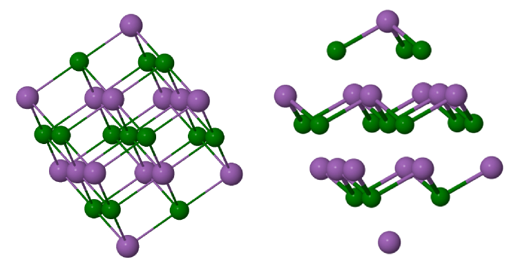
Figure 19: The structure of rhombohedral arsenic at normal conditions (r.h.s.) can be thought of as two superimposed face-centered cubic lattices, shown in purple and green, shifted relative to each other along the [111] direction. At sufficiently high pressures, the magnitude of the shift vanishes thus yielding the simple-cubic lattice (l.h.s.).

To extend the preceding notions to 3D materials we first note that the propensity of systems exhibiting substantial electronegativity variation to be insulators is not specific to a particular coordination pattern and is generic to any number of spatial dimensions; it is characteristic of many oxides and halides, for instance. In contrast, the Peierls instability is specific to one-dimensional systems, except in some idealized situations, such as when $sp$ mixing and $pp\pi$ interactions can be neglected, (burdett5764; burdett5774; BurdettLeePeierls) see also Refs. (PhysRevB.76.052301; SeoHoffmann1999; ZLMicro1) Here we take a phenomenological approach and simply use the experimental fact that rhombohedral arsenic becomes simple-cubic given sufficient pressure, (PhysRevB.77.024109; silas:174101) see Fig. 19. Alongside, the material undergoes an insulator-to-metal transition. (The self-consistent emergence of uniform, metallic bonding at high densities is consonant with the seminal ideas of Wigner (TF9383400678) and Mott, (0370-1298-62-7-303; Mott1990) of course.) Regardless of the precise mechanism of this electronic and mechanical instability, the formal reason why materials exhibiting bond-order CDW are insulating is a lack of electronic function overlap and, hence, lack of bonding within a significant subset of inter-atomic spaces. The latter subset houses the troughs of the off-site charge density wave, analogously to the Peierls-dimerized chain. Thus we identify the low mass density, low $\epsilon$ corner on our phase diagram of chemical interactions, Fig. 20, with an insulating phase characterized by a bond-order charge-density wave, in which both covalent and secondary interactions are generally present.

To estimate the location of the boundary, we assess the uniformity of bonding by computing the so called electron localization function (ELF).(Silvi1994) The ELF is determined by the curvature of the spherically averaged conditional pair probability for the electrons. By construction, the ELF varies between zero and one,(doi:10.1021/jp992784c) the two extremes corresponding to perfect localization and a uniform electron gas respectively. Surfaces of constant ELF=1/2 may be thought of as separating metallic and insulating regions.(doi:10.1021/jp992784c) The metallic regime sets in when the valence electrons percolate the space, see Fig. 21; conversely, there cannot be uniform bonding in the absence of the percolation. We have obtained the electronic wavefunctions for simple-cubic arsenic using the plane wave pseudo-potential method (PSPW) method in NWChem (Valiev20101477) and PBE96 exchange-correlation potential. A 64 atom repeat unit was used. We find that the percolation sets in very close to the experimentally known value (PhysRevB.77.024109; silas:174101) of the mass density at which elemental arsenic undergoes the rhombohedral-to-simple cubic transition. This is consistent with the expectation that the lack of connectivity in the valence electronic wavefunction will lead to a structural instability and, ultimately, regions of weak, secondary bonding. This is in full agreement with the results of Section III.

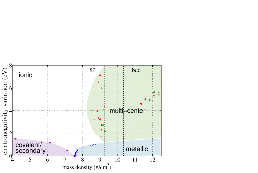
Figure 20: Phase diagram of chemical interactions. The abscissa corresponds with the mass density, assuming each atom has the same mass as arsenic. The ordinate gives the absolute value of the electronegativity difference $2\epsilon$ between pseudo-arsenic and pseudo-antimony atoms; the two artificial elements form either the simple-cubic (sc) or body-centered cubic (bcc) structure, by construction; the dashed lines delineate the coexistence of the two phases. The left-bottom corner is occupied by a relatively low-symmetry structure, such as rhombohedral arsenic, in which the bonding is spatially non-uniform. The $\epsilon=0$ end of its boundary matches that for the transition between rhombohedral and simple-cubic arsenic. See text for explanation of the symbols.

To estimate the mass density when such percolation takes place in the presence of electronegativity variation, we employ rock salt structures for the di-pnictogen compounds SbAs, BiAs, and BiP. The compounds were chosen to cover a broad range of electronegativity variation; note that AsP, BiAs and SbAs solids have been reported experimentally.(doi:10.1021/cm960606f) Since the phase diagram is constructed with two arsenics in mind, we must readjust our results to account for the difference in the atomic size and mass of the diatomic compounds from elemental arsenic. In view of our results for mixed-pnictogen trimers from the preceding Section, we used the ionic radii as the rescaling factor for the length. The so obtained points for the emergence of structural instability are shown with stars in Fig. 20. The points happen to fall onto a smooth line. Since to the left of the line, the density is too low to provide for bonding, the line gives an approximate bound on the mass density below which uniform bonding could not take place. Thus on the low density, low-$\epsilon$ side, the structure is characterized by a co-existence of (two-center) covalent and secondary bonding, as in the structure of rhombohedral arsenic, Fig. 19, or As₂S₃, Fig. 2(b). At the boundary and beyond, the bonding is expected to be more uniform. For instance, on the low $\epsilon$ end, it could be simple cubic, as in elemental arsenic or phosphorus. On the low density end, given large electronegativity variation, and for 1:1 stoichiometry, one could have the rock salt or CsCl structure, depending on the ion size ratio. Structures with lower point-symmetries can be envisioned, depending on the stoichiometry.

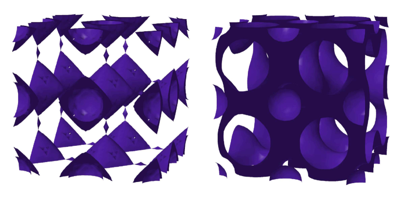
Figure 21: Left: The ELF=1/2 surface at the onset of metallicity. Right: The ELF=1/2 surface in the metallic regime. In both panels, the metallic and ionic regions are shown as filled and empty region, respectively. The cavities correspond to the ionic cores.

To extend the phase diagram in Fig. 20 to broader ranges in density and electronegativity variation, we will employ the following, unabashedly artificial device, as afforded by MOPAC: Imagine the rock salt structure, in which the anionic sites are occupied by arsenic, and cationic sites by antimony. Now increase the on-site energies for arsenic by $\epsilon$ upward so that the new value is $E^{\prime}_{\text{As}}=E_{\text{As}}+\epsilon$ for each orbital. At the same time, move all the antimony orbitals in energy so that they are $\epsilon$ below the unperturbed arsenic orbitals: $E^{\prime}_{\text{Sb}}=E_{\text{As}}-\epsilon$. Thus we impose an electronegativity variation entirely analogously to how it is done in the model Hamiltonian (9). Next, adjust the orbital exponents on the pseudo-antimony atoms so that the spatial dependences of Sb-As and Sb-Sb inter-orbital matrix elements fit maximally those of the corresponding As-As matrix elements. The resulting fit is good, but not perfect (see the Supplementary Material), because of the distinct angular dependences of the (valence) orbitals on As and Sb, which correspond to the principal quantum number $n=4$ and $n=5$ respectively. Lastly, make the Sb-Sb, Sb-As, and As-As ionic core repulsions identical while re-parametrizing them so that the density at which our hypothetical rock salt structure exhibits two transitions: the rhombohedral-to-simple cubic (rh-to-sc) and sc-to-bcc—both match their experimental values for elemental arsenic at $\epsilon=0$. The need for this re-parametrization is easy to understand since MOPAC’s default parameters are optimized for conventional pressures but do not necessarily account for the deformation of the ionic core at high pressures; further detail can be found in the Supporting Material. We reiterate that even at $\epsilon=0$, our pseudo arsenic and antimony are not strictly equivalent, because of the aforementioned difference in the angular dependence of the valence wavefunctions.

Now, to move vertically on the phase diagram one varies the quantity $\epsilon$; the quantity $2\epsilon$ is thus the externally imposed portion of the electronegativity differential between the cationic and anionic sites. The latter is the ordinate in Fig. 20 by construction. The horizontal axis corresponds with the mass density; the particle mass is set equal to that of arsenic for concreteness.

From here on, we limit ourselves to the area outside the covalent-secondary sector, the latter shown in lilac. One should expect a variety of structural transitions involving coordination changes as one moves about on the diagram. We will limit ourselves to just one such transition, viz., ’simple cubic’-to-’body centered cubic’ (sc-to-bcc), which is known to occur in elemental arsenic.(PhysRevB.77.024109) The latter transition is convenient for modeling pressure-induced coordination changes in that all bonds in the nearest coordination shell are equivalent in both structures, while the coordination itself changes meaningfully during the transition, viz., between 6 and 8. Away from the transition, we fix the structure to be rock-salt and cesium-chloride on the low and high density sides of the phase boundary, respectively; we vary only the density, not structure within individual phases. The (zero-temperature) transition is detected in the standard fashion, by computing the formation enthalpies of the two phases, as functions of volume, and finding the common-tangent to the two curves, (L_AP) see the Supplementary Material. This procedure amounts to mutually equating the pressures and chemical potentials of the two phases at zero temperature, aside from any error due to possible differences in the zero-point vibrational energies of the two structures. Because the transition is discontinuous in volume, there are actually a pair of phase boundaries, see Fig. 20, the two enclosing the phase-coexistence region; the latter is known to exhibit incommensurate host-guest structures. (PhysRevB.77.024109) We observe that the transition density is not sensitive to the value of the electronegativity variation. This lack of sensitivity likely indicates a limitation of our pseudo-pnictogen construct. Indeed, an ionic crystal with stoichiometry 1:1 and comparable sizes of the cation and anion is expected to have the CsCl structure at ordinary densities. The rock salt structure would require negative pressure or sufficient mismatch in the ion sizes.

Nonwithstanding its limitations, our artificial procedure allows one to monitor, even if qualitatively, charge redistribution in response to changes in density, electronegativity variation, and coordination. To quantify the spatial distribution of the frontier electrons, we directly compute the (average) excess charge $\Delta\rho$ on the more electronegative element relative to the less electronegative element. The amount of charge on an atom is determined by adding the diagonal entries of the density matrix pertaining to the $s$, $p$, and $d$ orbital on that atom. The charge differential $\Delta\rho$ gives the strength of the on-site charge density wave. Near the horizontal axis on the diagram, $\epsilon=0$, $\Delta\rho$ is small, which we associate with metallic bonding in the absence of a bond-order wave. Conversely, at large values of $\epsilon$, the quantity $\Delta\rho$ is large, implying ionic bonding. Because the quantity $\epsilon$ couples linearly to the electron density, as in Eq. (9), the following statement holds:

$$\Delta\rho=-\frac{\partial E}{\partial\epsilon},$$ (12)

where $E$ is the exact energy of the system per atom. (This can be shown explicitly using Eq. (11.16) of Ref. (LLquantum).)

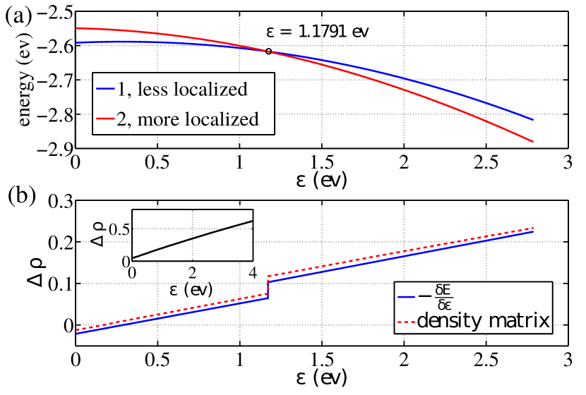
Figure 22: (a) A specific instance of term-crossing for the ground state of the pseudo-pnictogen compound from Fig. 20. (b) The corresponding dependence of the electron density differential $\Delta\rho$ as determined directly using MOPAC-computed density matrix and by numerically differentiating the $E(\epsilon)$ curves from panel (a). The differentiation was performed using the best parabolic fit to the $E(\epsilon)$ curves. Although numerically similar, the two curves are not identical because MOPAC does not solve the Schrödinger equation exactly.

We next prepare our pseudo-pnictogen sample at distinct values of the density and electronegativity variation, by performing $\epsilon$ sweeps from $2\epsilon=0$ to $8$ eV, while keeping the density fixed. The sample size is 64 atoms for the sc structure, 54 atoms for the bcc structure; the finite size effects are treated according to a standard procedure. (PerkinsStewart1980) We observe that below a certain threshold density, the energy and wavefunction of the system depend smoothly on the value of epsilon. Above that threshold density, the dependence becomes more complicated. The sample can now transition between distinct energy terms, as in Fig. 22(a). Each term crossing is accompanied by a discrete change in charge distribution, see Fig. 22(b). Because of such crossings, the wavefunction and energy show a hysteretic behavior during $\epsilon$ sweeps (see the Supplementary Material). The locations of the corresponding term-crossings can be detected; some are indicated on the phase diagram in Fig. 20 with the triangles.

These transitions were anticipated by Kohn a while ago (PhysRevLett.19.789; PhysRevLett.19.439) in the context of the metal-insulator transition and are generally expected for solids exhibiting conduction and valence bands with distinct anisotropies. In the picture advanced by Kohn, the canonical metal and insulating states are separated by a chain of consecutive transitions that mutually stabilize distinct sets of electrons and holes. Here we observe a noteworthy situation that term crossings (at the ground state energy) begin to occur only above a certain value of mass density. Two states corresponding to two different energy terms may be regarded as distinct phases corresponding to distinct degrees of electron localization. This is brought home by introducing the Legendre transform of the energy, $E^{\text{(inh)}}(\Delta\rho)$, which can be treated naturally as a function of $\Delta\rho$:

$$E^{\text{(inh)}}(\Delta\rho)=E[\epsilon(\Delta\rho)]+\epsilon(\Delta\rho)\,\Delta\rho,$$ (13)

where

$$\epsilon(\Delta\rho)=\frac{\partial E^{\text{(inh)}}(\Delta\rho)}{\partial\Delta\rho}.$$ (14)

The label “inh” signifies that the thermodynamic potential $E^{\text{(inh)}}(\Delta\rho)$ is inherently a functional of the electronic density distribution. The existence of such a functional is guaranteed by the Hohenberg-Kohn theorem. (PhysRev.136.B864) In such a density-based approach, (L_AP) one can unambiguously determine the field necessary to achieve a specific strength of the CDW if desired, via Eq. (14). The thermodynamic potentials $E^{\text{(inh)}}(\Delta\rho)$ and $E(\epsilon)$ are analogous to the Helmholtz and grand-canonical free energy, respectively. (CL_LG)

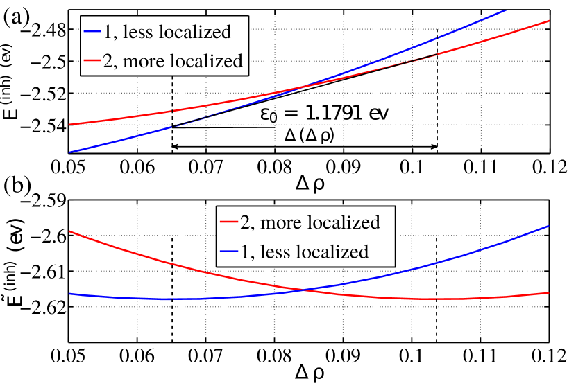
Figure 23: (a) The inherent electronic energy from Eq. (13) as a function of the electron density differential $\Delta\rho$, corresponding to Fig. 22. (b) The modified energy $\widetilde{E}^{\text{(int)}}(\Delta\rho)\equiv E^{\text{(int)}}(\Delta\rho)-\epsilon_{0}\,\Delta\rho$ whose minima correspond to the equilibrium values of $\Delta\rho$ when the externally imposed electronegativity variation is equal to $\epsilon_{0}$. The locations of the minima are indicated with the dashed lines.

Fig. 23(a) displays the term crossing from Fig. 22 in terms of the inherent energy $E^{\text{(inh)}}(\Delta\rho)$, at mass density 9.01 g/cm³. The latter figure explicitly illustrates a discontinuous transition between two states, where the quantity $\epsilon_{0}$ gives the slope of the common tangent to the two terms. Particularly illuminating is the graph of the quantity $\widetilde{E}^{\text{(inh)}}(\Delta\rho)\equiv E^{\text{(inh)}}(\Delta\rho)-\epsilon_{0}\,\Delta\rho$, where $\epsilon_{0}$ is a constant, not a function of $\Delta\rho$; see Fig. 23(b). When the conditions for equilibrium for any pair of states are met, the two minima of $\widetilde{E}^{\text{(inh)}}(\Delta\rho)$ corresponding to the states have the same depth. Note that the term crossing in Fig. 23 is only possible because there are more than one orbital per site. Otherwise, the variable $\Delta\rho$ would specify the charge distribution uniquely, which would then imply that to the same density distribution, there correspond more than one energy functional, a physical impossibility. (PhysRev.136.B864) We have checked that the individual contents of the $s$, $p$, and $d$ orbitals corresponding to the two terms in Fig. 23 do exhibit discontinuities at the term crossing.

The l.h.s. and r.h.s. minima in Fig. 23(b) correspond to states with a lesser and greater degree of electron localization. The presence of a barrier separating those states can be traced to a very familiar phenomenon, viz., the lack of mutual miscibility of oil and water. Indeed, states characterized by distinct degrees of electron localization will also exhibit distinct polarizabilities, hence the analogy. The hysteretic region on the phase diagram formally corresponds to a coexistence of two phases. The coexistence region exhibits an electronic pattern that interpolates between those typical of metallic and ionic bonding, the two formally corresponding to maximally extended and localized bonding orbitals, respectively. Thus we identify the ionic/metallic coexistence region with the intermediate case of the multi-center bond, see also the discussion in Section V.

We emphasize that although we have treated local electronegativity as a continuous variable, in practice the choice of $\epsilon$ is limited to that afforded by specific chemical elements. The presence of discontinuous transitions of the kind shown in Fig. 23 indicates an additional complication for the materials chemist: Even if realizable chemically in principle, a specific value of electronegativity variation may not be achievable in an actual compound, if the resulting charge density wave with a spatially uniform strength is unstable toward phase separation. In the best case scenario, the compound will be a collection of stripes whose CDW strength alternates between $\Delta\rho_{1}$ and $\Delta\rho_{2}$. In the worst case, the compound will not form altogether. Conversely, no such complications arise at sufficiently low mass densities.

The present calculations thus indicate that depending on the density, a transition between states with distinct magnitudes of the CDW can be generally either continuous or discontinuous. This means, in particular, that the metal-insulator transition can be either continuous or discontinuous. (Note we are not considering effects of disorder. (PhysRevLett.42.673; Mott1993)) The possibility of a continuous localization transition in electronic systems is in contrast with classical liquids made of rigid particles, which always solidify discontinuously. (LandauPT1; Brazovskii1975; dens_F1; L_AP) These contrasting behaviors may come about for the following reason: Rigid particles create a bounding potential for each other in a self-consistent fashion; there is no other source of particle confinement. In contrast, electrons in solids are subject to a field due to largely stationary nuclei. This field already lowers the full translational symmetry that would have been present in a weakly interacting electron gas, the precise extent of symmetry-breaking determining whether electric conductance vanishes. Incidentally, note that the transition in Figs. 22 and 23 is only weakly discontinuous; its analog in an actual material may not be easily distinguished from a continuous transition or a soft crossover.

As a consistency check, we have tested the stability of our pseudo-pnictogen rock salt structure with respect to deformation toward the rhombohedral structure, Fig. 19, see details in the Supplementary Material. This instability line, shown with circles in Fig. 20, is seen to lie under the ionic-metallic coexistence region. On the one hand, this implies the propensity for electron localization (or lack thereof) in symmetric structures is deeply connected to structural instability, as was anticipated by Kohn. (PhysRevLett.19.789; PhysRevLett.19.439) On the other hand, the instability implies that in a proper treatment, the CDW pattern and lattice must be determined self-consistently.

In parallel with Section II, we now address the interplay of cohesive and repulsive interactions during density-driven transitions accompanied by coordination changes. The strengths of the two interactions often move in the same direction: Both the electron density in the inter-atomic space and the repulsion between the ionic cores tend to increase with density. A qualitative, Le Chatelier-like criterion can be stated for whether a change in coordination is driven primarily by steric repulsion or cohesive interactions. First note that the interatomic distance $r$ can either decrease or increase upon a discontinuous volume change. For instance, it is easy to convince oneself that the following simple formula interpolates the relation between the specific volume $v$ and coordination number $n$ for the diamond, simple cubic, and bcc lattice: $r\approx[0.16vn]^{1/3}$, ($n\leq 8$). Now, consider a pressure-driven transition with $\Delta v<0$ and $\Delta n>0$. If the distance $r$ increased, then the increase in the coordination was to counteract the effects of steric repulsion; hence the latter can be cited as the dominant factor in the coordination increase, while the reverse transition can be thought of as driven by cohesive interactions. For instance, for a pressure-driven sc-to-bcc transition, $n_{\text{bcc}}/n_{\text{sc}}=4/3$. For such a transition to be driven by cohesive forces, the volume decrease would have to be 25%; we are not aware of such large density changes for phase transitions in condensed phases. In contrast, for the bcc-to-fcc transition, $r_{\text{fcc}}/r_{\text{bcc}}\approx(1.09\,v_{\text{fcc}}/v_{\text{bcc}})^{1/3}$, and so already a 10% change in volume would imply cohesive interactions are important. An elegant discussion of pertinent electronic processes can be found in Ref. (doi:10.1021/ja0114557)

The above ideas help to resolve a seeming contradiction (see also a discussion in Ref. (ANIE:ANIE200602485)): On the one hand, there is an empirical correspondence rule stating that lighter elements under high pressures tend to form structures typical of elements down the group at normal pressures. (ISI:000077643800009; ANIE:ANIE200602485) At the same time, heavier elements tend to exhibit less $sp$-mixing and higher coordination, (PapoianHoffmann2000; doi:10.1021/ja0032576) the di-pnictogen tri-chalcogenides representing a good example, (ZLMicro1) as in Fig. 2. On the other hand, we have seen that the amount of $sp$-mixing should increase with density. This seeming contradiction may be resolved in the following way: The $sp$-mixing should indeed increase with density for a fixed or mildly deforming structure. Eventually, however, a density driven structural transition causes a coordination increase that leads to a longer bond and lesser amount of $sp$-mixing. It is this kind of transition that underlies the general trend that the amount of $sp$-mixing should decrease with mass density.

The increased coordination on the one hand, and the decreased amount of bond directionality (caused by $sp$-mixing) on the other hand, are hallmarks of the metallic interactions. Thus we identify the high density, $\epsilon\to 0$ limit with metallic interactions and delocalized electrons. We reiterate that the low and high density limit, for sufficiently low $\epsilon$, should correspond to insulating and metallic behaviors on general grounds. (TF9383400678; 0370-1298-62-7-303; Mott1990) Now, for any value of density, one may always choose a large enough electronegativity difference to force the valence electrons to localize on the more electronegative atoms. Thus we identify the $\epsilon\to\infty$ limit with the ionic bond and conclude that the coexistence region widens, in terms of $\epsilon$, with density. The above reasoning does not straightforwardly apply when some bonds become shorter and others longer with density changes, as in the covalent-secondary sector in Fig. 1. At least in the case of rhombohedral arsenic, it is still possible to argue, see the Supplementary Material, that the amount of $sp$-mixing decreases with density.

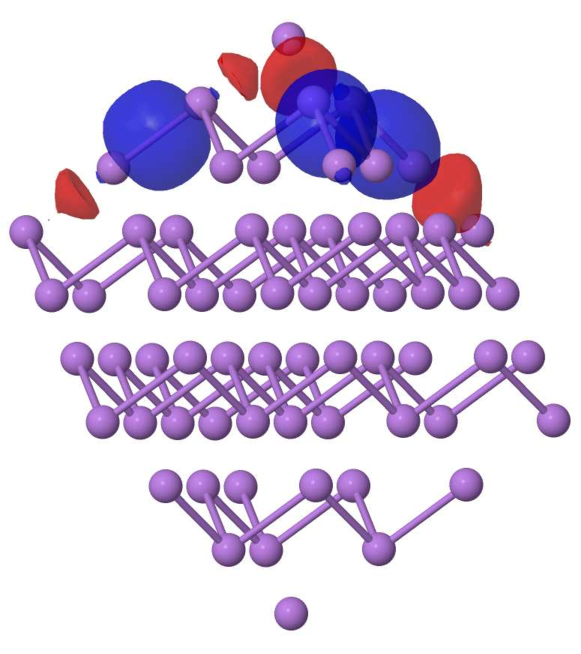
Figure 24: Examples of the LMOs obtained for a specific HF solution for elemental arsenic arranged in the simple-cubic structure, indicated by the spheres. The HF procedure was seeded by the solution for rhombohedral arsenic, see text for explanation. Each link denotes where a two-center LMO is present; only three LMOs are actually shown, to avoid crowding. The link pattern clearly following the bond pattern of rhombohedral arsenic.

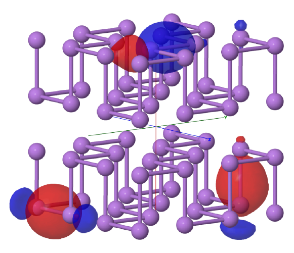
Figure 25: Same as Fig. 24, but with the HF solution obtained by using the black phosphorus structure as the seed.

We finish by displaying some of the CDW patterns that emerge in the solid state at the single Slater-deteminant level as a result of Kohn-like transitions. Here we use MOPAC and the LMO formalism to describe bonding in an extended sample of simple cubic arsenic, see Figs. 24 and 25. The molecular orbitals are built for a modestly-sized repeat unit, which we chose to be a $4\times 4\times 4$ cube; the crystal field of an infinite solid is inferred by MOPAC according to a procedure explained in Ref. (JS556) Already in this caricature solid, we find that the search for the true lowest energy HF-solution often becomes impractical. The result of the calculation depends on the initial guess for the wavefunction. We limit ourselves to two specific initial guesses by first creating lower-symmetry structures, namely, rhombohedral arsenic and black-phosphorus. Then, we gradually move the nuclei toward their positions in the simple-cubic structure, while recomputing the wavefunction at each step using the result from the preceding geometry as the initial guess for the SCHF procedure. We find that the CDW that appears to be the likely true ground state for the symmetry-broken nuclear configuration persists even in the symmetric, simple-cubic nuclear configuration. The resulting LMOs are shown in Fig. 24 and 25 for the rhombohedral arsenic and black phosphorus seed, respectively. The mass density employed in these calculations is 5.89 g/cm³, which is just above the experimental value of 5.75 g/cm³ for rhombohedral arsenic at normal conditions and well below the density of simple-cubic arsenic, viz., 7.48 g/cm³. We observe that the two-center LMOs cover only a half of the nearest-neighbor spaces, consistent with the experimentally known fact that simple-cubic arsenic is unstable toward a displacive transition at ambient pressure. (silas:174101; PhysRevB.77.024109) We have also found that in the absence of deliberate “seeding,” the “classical” HF solution spontaneously acquires the symmetry of rhombohedral arsenic, at sufficiently low densities. This suggests that at least in some cases, the solution of the Hartree-Fock problem for an unstable, symmetric atomic arrangement may may predict the geometry of the actual, symmetry-lowered structure

V Discussion

The present results demonstrate the inherent relation and, at the same time, distinction between fundamental chemical forces. Both the type and strength of the chemical bond are established as a result of phase transitions resulting from charge redistribution. The canonical chemical interactions are shown to underly distinct thermodynamic phases and thus can be viewed as distinct sectors on a phase diagram. We have argued that in the most minimal description, such a phase diagram is in the space formed by two variables, particle density and local electronegativity variation. The conventional, two-center covalent bond and closed-shell interactions can be thought of as mutually-complementary, intrinsic counterparts that occupy the very same sector on the phase diagram of chemical interactions. The intrinsic connection between the covalent bond and closed shell interactions is that the two are symmetry broken versions of the multi-center bond. In turn, the multi-center bond can be thought of as a coexistence, or hybrid, between the metallic and ionic bond.

The metallic and ionic bond thus emerge as the two most fundamental interactions that become entirely distinct in the high density limit. The distinction can be understood qualitatively as poor mutual miscibility of delocalized and localized electrons. The former can be thought of as an electron fluid that can flow despite the partial breaking of the translational symmetry due to the nuclei. In insulators, the translational symmetry breaking is complete. Phase separation in electronic systems and associated striped phases has been reported by Schmalian and Wolynes, (SWmayo) who have suggested such separation is pertinent to metal ammonia solutions and high $T_{c}$ superconductors alike. The present model analysis shows the distinction between the metallic and ionic interactions decreases as the density is lowered, until the two become two opposite limits of a continuum of interactions. At lower yet densities, the number of electrons in the inter-atomic space becomes insufficient to support the multicenter bond; the latter thus breaks into the covalent bond and the closed-shell interactions, provided the electronegativity variation is not too large. The resulting charge-density wave can be thought of as a bond-order wave.

That changes in bond order in small molecules should be analogous to phase transitions can be viewed as a limiting case of the results obtained for bulk samples. This notion is consistent with the finite-size-scaling philosophy of bonding and dissociation due to Kais, Herschbach, and others. (KaisSerraACP; doi:10.1063/1.1637581) Here we observe that changes in bond order are associated with transitions in the strength, but also symmetry of the charge density wave. Discrete changes in bond order come about naturally in venerable theories of bonding, such as the molecular orbital theory or the early ideas of G. N. Lewis. Bond breaking during molecular dissociation is often viewed as a term-crossing event that occurs provided the ground and an excited state molecular term switch their identities at separations beyond a certain threshold value. (LLquantum) The “sharpness” of the transition transition depends on the strength of coupling between the two terms at the crossing point. Yet already for modestly sized molecules, let alone solids, the spacing between molecular terms becomes very small making it difficult to identify term crossings. Instead, we take the charge density wave (CDW) perspective, (gruner2009density; CanadellWhangbo1991) which itself is rooted in the venerable density functional theory (PhysRev.136.B864; PhysRev.140.A1133) The Coulomb attraction to the nuclei and the electron-electron repulsion favor electron localization; the delocalization is driven by minimization of the kinetic energy. The interplay of these opposing forces gives rise to a variety of CDW patterns; each pattern is associated with a specific bond-order assignment. Transitions between respective patterns turn out to be well defined. Localized molecular orbitals (LMOs) represent a particularly convenient way to monitor and visualize how the bonding electrons are redistributed during those transitions. Unlike the canonical MOs, the LMOs are not required to comprise irreducible representations of the molecule’s symmetry group and are more prone to symmetry changes.

The similarity in behavior between distinct HF-derived CDW states in small molecules, on the one hand, and thermodynamic phases, on the other hand, is not surprising on formal grounds. The Hartree-Fock derived electronic energy $E$, for a finite basis-set, is a minimum of a quartic polynomial made of expansion coefficients such as the $\widetilde{C}$s from Eq. (3); the fourth-order terms come from the electron-electron interactions. Clearly, such a polynomial will exhibit a myriad solutions already for modestly sized molecules. Distinct solutions are often separated by barriers, hence the discontinuous transitions discussed above. Continuous transitions are somewhat less common but will still take place when the Jacobian $\partial^{2}E/\partial\widetilde{C}_{i}\partial\widetilde{C}_{j}$ computed at the minimum in question vanishes. This is quite similar to how one may describe macroscopic phase transitions at a meanfield level using the Landau-Ginzburg classical density functional theory. (Goldenfeld) The CDW perspective suggests that the connection between the present results and macroscopic phase transitions is not only formal but stems from the intrinsic propensity of mutually repulsive particles to localize or delocalize in a cooperative fashion. (L_AP)

The interatomic spacing is a natural lengthscale in bonded systems; it is, in turn, largely determined by the Bohr radius. Structures characterized by supra-atomic lengths can be often thought of as made of small “building blocks” that are perturbed only weakly when the solid is assembled; this is the case with many oxides and halides, for instance. Complex inorganic solids made of individually stable subunits can have unit cells that contain as many as tens of thousands of atoms. (Weber:sn5082; Dshemuchadse:sn5123) Alternative types of ordering are possible—even if on a modest length scale—where the type of bonding within the building blocks will depend on whether the blocks are standalone or bonded relatively intimately, as in Fig. 2(a). This indicates that there is an emergent length scale in condensed phases that is not directly tied to the atomic scale. Kohn designated such ordered structures “superlattices,” which could arise, in principle, during a series of transitions separating the canonical metallic and insulating states. (PhysRevLett.19.789) Consistent with those early ideas, such supra atomic length scales emerge in the present picture as widths of interfaces separating states with distinct CDWs—or distinct chemical interactions—that coexist spatially. The simplest formalism to describe such a coexistence is via the Landau-Ginzburg free energy functional: (CahnHilliard; RowlinsonWidom; Bray; CL_LG)

$$F=\int dV\left[\frac{\kappa}{2}(\nabla\phi)^{2}+{\cal V}(\phi)\right],$$ (15)

where $\kappa>0$ is a phenomenological coefficient reflecting the free energy penalty for spatial inhomogeneity in the order parameter $\phi$. The bulk free energy density ${\cal V}(\phi)$ has two or more minima corresponding to coexisting phases, such as that in Fig. 23.

Sufficiently far from the critical point, the meanfield description embodied in the functional (15) becomes quantitative; the interface width $l_{\text{intf}}$ scales roughly as $(\kappa/g^{\ddagger})^{1/2}$, where $g^{\ddagger}$ is the height of the barrier in the bulk energy density ${\cal V}(\phi)$ that separates the corresponding pair of phases. The interface tension coefficient is of the order $(\kappa g^{\ddagger})^{1/2}$. At the critical point, which formally corresponds to the $g^{\ddagger}\to 0$ limit, the meanfield approximation is only qualitative, however it still correctly predicts that the interface width diverges, while its tension vanishes. The correlation length also diverges at the critical point and so does the susceptibility, (Goldenfeld) implying a structural instability, such as that at the simple cubic-to-rhombohedral transition in elemental arsenic. It is thus likely that in actual materials, which form subject to many perturbations, the length scale associated with the coexistence will always remain finite. Consequently, the hybrid of the metallic and ionic bond is the multi-center bond. The latter is directional, even if its progenitors are not. The directionality comes about already because of the stiffness of the interface; the presence of the interface breaks the isotropy of space. These ideas are consonant with the classic explanation of bond directionality via hybridization of atomic orbitals.

The interface width decreases with separation from the critical point; once the width becomes less that the interparticle-spacing, there are at least two alternative possibilities: At low densities (or for lighter elements), the multi-center bond is replaced by a coexistence of the two-center covalent bond and secondary interactions, as in Fig. 2(b). The Bi₂Te₃ structure in Fig. 2(a) corresponds to intermediate densities; here the multicenter bond is still present and forms an interface between covalent/secondary regions. Exclusively covalent bonding is also possible for particular electron counts, as in the diamond structure. (Still, the C-C bond length in diamond is longer than that in graphene.) At higher densities, metallic and ionic interactions become well-defined individually, but could also spatially coexist as in layered compounds where current is purveyed within select layers.

One thus arrives at the notions of the familiar two-center bond and bond directionality—intrinsically atomistic concepts—starting from a coarse-grained picture, such as that described by the (classical) density functional in Eq. (15). Such a coarse-grained view is far from new; it underlies the venerable density-functional theory, (PhysRev.136.B864; PhysRev.140.A1133) of course. Here, we find that some results of classical density functional treatments are transferable to electrons, such as poor miscibility of localized and delocalized particles. The Heusler and half-Heusler compounds, and incommensurate phases seem to exemplify such poor miscibility, as mentioned ealier. Furthermore, the idea of coarse-graining is central to the renormalization group (RG) theory of phase transitions. Coarse-graining transformations can be thought of as movement in the space defined by coupling constants. (Goldenfeld) Distinct phases come about as attractive fixed points for such transformations. The present results suggest the ionic, metallic, and covalent/secondary interactions are such attractive fixed points, the latter essentially corresponding with the corners of the venerable Arkel-Ketelaar triangle. (doi:10.1021/ed012p53; vanArkel; Ketelaar; Burdett1995)

Laws of corresponding states arise when the system is close to a critical point, where the RG flows of the coupling constants are not sensitive to system-specific detail but only to the symmetry and range of interactions because the correlation length now greatly exceeds molecular lengthscales. Long wavelength, possibly disordered patterns that may arise as a consequence of such instabilities are difficult to predict using ab initio methods, because the size of the repeat unit, if any, of the distorted structure is not a priori known. Examples of such complex distortions of recent note are represented by hybrid organic-lead halide perovskites (doi:10.1021/acs.jpclett.6b01648) and oxide-ion conducting perovskite derivatives. (doi:10.1021/jacs.6b10730) It is quite possible that the multiplicity of mutual orientations of rigid molecular units in those compounds, such as octahedra or tetrahedra, scales exponentially with the sample size thus limiting the utility of brute force, ab initio approaches. A hybrid strategy seems more profitable, in which one uses ab initio methods to infer the parameters for a coarse-grained description in the form of a free-energy functional, such as those that have been used to study displacive transitions and multiferroic behavior. (PhysRevLett.3.412; Dove1997) (Examples of such inference for simple liquids and spin systems can be found in Ref. (L_AP)) The resulting functional can be tested, in principle, for the multiplicity of states. (MP_Wiley; SchmalianWolynes2000; BL_6Spin; PhysRevB.91.100202) Conversely, textbook approximations to canonical bonding schemes should work close to attractive fixed points. Near phase boundaries—not too close to critical points, if any—one should expect ordering on supra-atomic length scales.

Of course the present, coarse-grained view of the chemical interaction cannot replace detailed quantum-chemical analyses for the stability of known compounds. Rather, we believe the present findings complement those detailed analyses and, in particular, may provide an additional tool for predicting novel compounds. For instance, the density-functional perspective may help one to predict whether specific ingredients will bind to form a stable or metastable solid, as opposed to segregating into unwanted products. Indeed, insofar as localized electrons are tied to regions with significant electronegativity variation—and vice versa for the delocalized electrons—the mutual miscibility of the corresponding moieties is tied to that of the respective electronic subsystems. The latter mutual miscibility seems a natural variable for machine-learning algorithms that have been used for predicting the existence and properties of compounds. (Dyer17052013; 2178621820060801; Villars200126) The present results also suggest that multiferroic materials and any other solids prone to structural instabilities should be relatively close to the critical points and phase boundaries on the phase diagram in Fig. 20. Note that while achieving uniformly high densities in the bulk may require substantial compression, locally-dense environment can be created using chemistry even at normal conditions, for instance, by substituting elements by their heavier neighbors down the group.

The present results on specifics of electronic localization already suggest a concrete way to speed up search for stable geometries. We have seen that already in the symmetric, simple cubic structure of arsenic, the LMOs predict the actual distorted structure without the need for costly geometric optimization. This suggests a way to efficiently screen very large numbers of candidate compounds for stability and possible isomers. In this procedure, a computer first generates a variety of structures for a molecule or solid alike, subject only to steric constraints. The candidate structures may be relatively symmetric, thus greatly reducing the pool of trial configurations. In the next step, a computationally efficient, semi-empirical approximation is used to obtain the molecular orbitals, after which the localized molecular orbitals are generated. (Both functionalities are already implemented in MOPAC, for instance.) If the two-center LMOs happen to cover inter-atomic spaces within a sufficiently large fraction of nearest neighbors, the candidate compound and structure are rated as a high probability target for further screening. Indeed, since every nearest neighbor bond is covered by a two-center LMO, one may expect the putative geometry to be either stable or metastable. If, on the other hand, the coverage is not complete, the nuclear configuration is expected to distort so as to follow the electronic instability. If, furthermore, there are more than one equivalent yet distinct coverage patterns, then we arrive at the venerable notion of a resonance. (PaulingBond; doi:10.1021/cr100228r) The resulting distorted geometries may or may not be separated by a barrier surmountable by zero-point molecular vibrations, the former and latter cases exemplified by ammonia and trans-polyacetylene, (RevModPhys.60.781) respectively. The candidate compounds may be also generated subject to preset constraints of interest in specific applications, such as the design of a docking site for a given ligand of interest. These ideas should be suitably modified for bonding involving $d$ and higher order orbitals and for coordination numbers exceeding six; this is work in progress.

Supplementary Material

The Supplementary Material is organized by Section of the main text and contains supporting grahics and discussion on: Potential energy surfaces of the trimers; effects of zero-point vibrations, electronegativity varation, and electron count on symmetry breaking; and lack of promotion of core electrons (Section II). Pedagogical review of the LMO formalism; additional aspects of the LMO and stability analysis for trimers and 20-member ring; and NBO and QTAIM perspective on the dissociation of the trimer (Section III). Details of MOPAC re-parametrization, and $sp$-mixing in bulk arsenic (Section IV).

Acknowledgments: We thank Peter G. Wolynes, Eric Bittner, Arnold Guloy, Zhifeng Ren, and J. J. P. Stewart for discussions and insight. This work has been supported by the National Science Foundation Grants CHE-0956127, CHE-1465125, and the Welch Foundation Grant E-1765. The authors acknowledge the use of the Maxwell/Opuntia Cluster and the advanced support from the Center of Advanced Computing and Data Systems at the University of Houston. The authors acknowledge the Texas Advanced Computing Center (TACC) at The University of Texas at Austin for providing HPC resources. URL: http://www.tacc.utexas.edu.

^† Present address: UT Southwestern Medical School; Dallas, TX 75390-9003

I Potential energy of the $\text{AsH}_{2}-\text{AsH}-\text{AsH}_{2}$ trimer

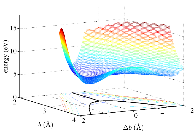
Figure S1: Potential energy surface for the linear 3/4 trimer AsH₂-AsH₁-AsH₂ as a function the displacement $\Delta b\equiv(b_{2}-b_{1})/2$ of the central As atom off the trimer’s midpoint and the chain length per bond $b\equiv(b_{1}+b_{2})/2$. The quantities $b_{1}$ and $b_{1}$ stand for the As-As bond lengths. The minimum energy contour, shown in bold on the contour plot beneath the surface, is determined by minimizing the energy at a fixed value of $b$. The surface was obtained using the semi-empirical quantum-chemistry package MOPAC with PM6 parametrization.(JS12)

II Fluctuation-induced lowering of the symmetry breaking

The potential energy surface in Fig. S1 was obtained using the Born-Oppenheimer approximation; its minima determine the zero-temperature location of the nuclei in the classical limit. A slice of the energy surface in the symmetry-broken region, at a constant value of the overall trimer length, is exemplified in Fig. S2 by the solid line. Already zero-point vibration will be sufficient to overcome the barrier separating the two minima on the bistable energy profile, provided the barrier is sufficiently low. To determine qualitatively the trimer length where the barrier can be still overcome by zero-point vibrations, we consider the symmetric stretch for concreteness. A harmonic oscillator with frequency $\omega$ and mass $m$ exhibits zero-point vibrations of magnitude (LLquantum)

$$x_{T=0}=\left(\frac{\hbar}{m\omega}\right)^{1/2}.$$ (S1)

For a quadratic potential whose force constant $\kappa$ matches the curvature of a symmetry-broken minimum, $\omega=(\kappa/m)^{1/2}$, where $m$ is the mass of a terminal atom. Next, we find the value of the trimer length at which the vibrational magnitude (S1) exactly matches the half-width of the barrier separating the two minima, see the graphical explanation in Fig. S2. This length is indicated with the asterisk on Fig. 4 of main text.

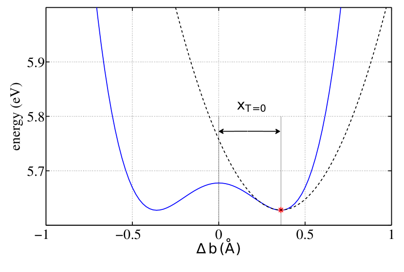
Figure S2: The solid line is a slice of the potential energy function from Fig. S1. The location of the slice is chosen so that zero-point vibrations in the harmonic potential approximating a metastable minimum on the actual potential surface do not exceed, in magnitude, the half-width of the barrier separating the two minima on the symmetry broken energy surface.

III Lack of promotion of $3d$ electrons

It is desirable to check how much the outermost filled $d$ shells are modified following contraction of the trimer, to test whether MOPAC’s (JS12) implicit treatment of the core electrons introduces substantial error. To this end, we perform an all-electron HF calculation using the package Orca. (PN137; Libint2) We consider a trimer at low density and identify the molecular orbital, call it X, that primarily consists of the $3d$ atomic orbitals. We next compress the trimer and, alongside, monitor the contribution of the atomic $3d$ atomic orbitals to the molecular orbital X. This contribution is shown in Fig. S3 with circles. We observe that the atomic $3d$ orbitals do not contribute substantially to the bonding orbitals even at relatively high densities. For the sake of comparison, we also show the contribution of the atomic $4s$ orbitals to the very same molecular orbital, with the squares.

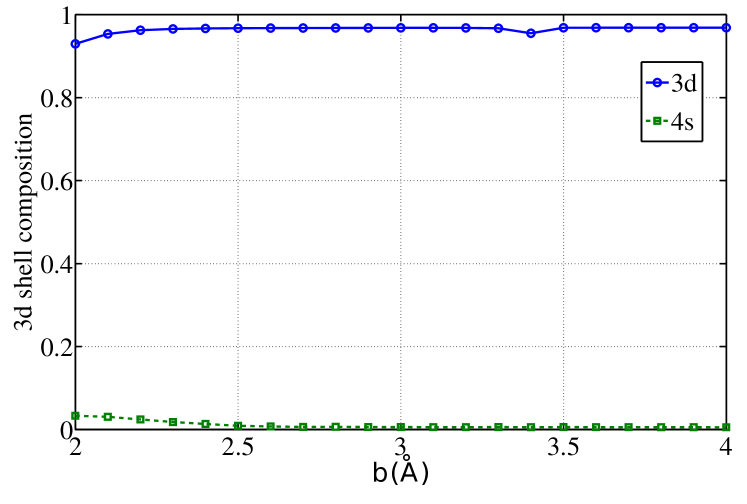
Figure S3: Fractional contribution of atomic $3d$ and $4s$ orbitals to the trimer’s molecular orbital that can identified as primarily consisting of $3d$ atomic orbitals at low densities. The horizontal axis is the trimer length per bond. The trimer is the linear 3/4 molecule AsH₂-AsH₁-AsH₂. The calculations were performed with all-electron HF calculation as implemented in the package Orca. (PN137; Libint2)

IV Dependence of symmetry breaking on the $pp\sigma$ bond electron count

The symmetry-breaking graphs for three values of electron count in the linear trimer AsH₂-AsH_n-AsH₂, $n=0,1,2$, indicate that the symmetric state becomes less stable when the electron count differs from its ideal value of four, which yields perfect Lewis octets for each arsenic. (This situation is realized for a singly-hydrogenated central arsenic, $n=1$.) In addition, we observe that in contrast with the situations shown in Fig. 4 and 10 of the main text, the critical length is no longer the only characteristic length in the problem. The three bifurcation graphs, shown in Fig. S4, can still be rescaled so as to follow one universal curve, inset of Fig. S4, however doing so requires two independent lengths, one needed to fix the lateral position of the critical point, the other to fix the strength of symmetry breaking.

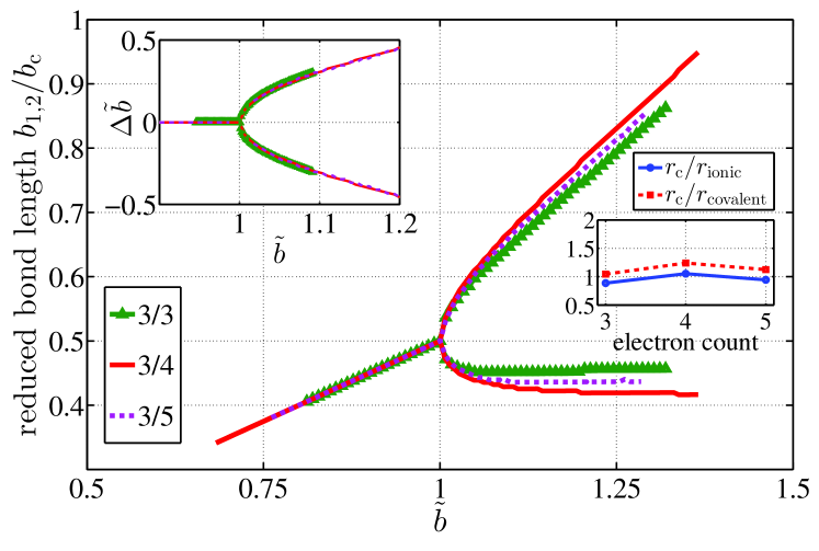
Figure S4: Bond lengths for three arsenic trimers, AsH₂-AsH_n-AsH₂ trimer, as functions of the overall trimer length per bond. The three cases, $n=0,1,2$, correspond to a five, four, and three electron $pp\sigma$ bond bond, respectively. Both axes are scaled by the corresponding critical bond length $b_{c}$. Additional scaling is needed to bring the three curves to one universal dependence.

V Effects of electronegativity variation

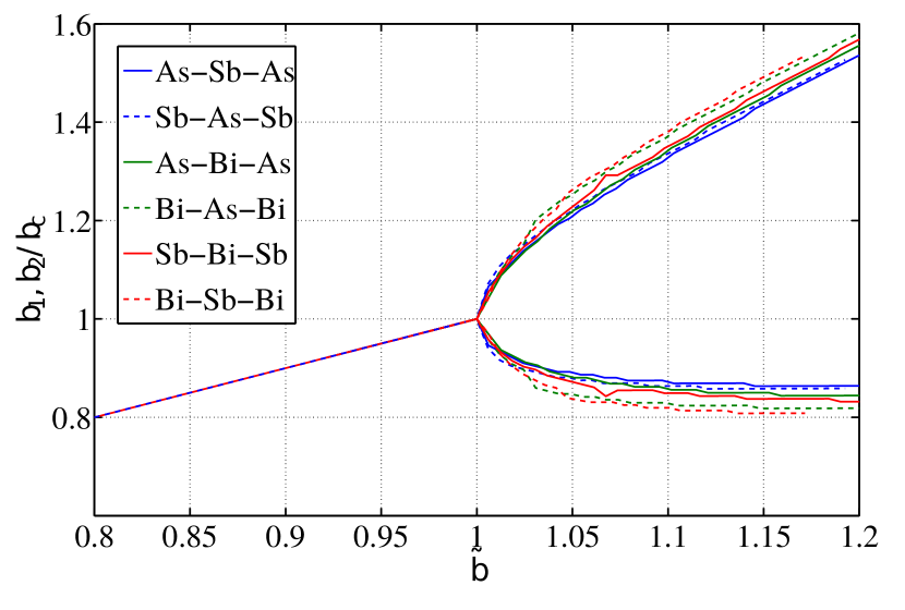
Figure S5: Bond lengths for several heteronuclear 3/4 trimers XH₂-YH₁-XH₂ and YH₂-XH₁-YH₂, as functions of the overall trimer length per bond. Both axes are rescaled by the corresponding critical radii, no additional rescaling of the $\Delta b$ coordinate was performed.

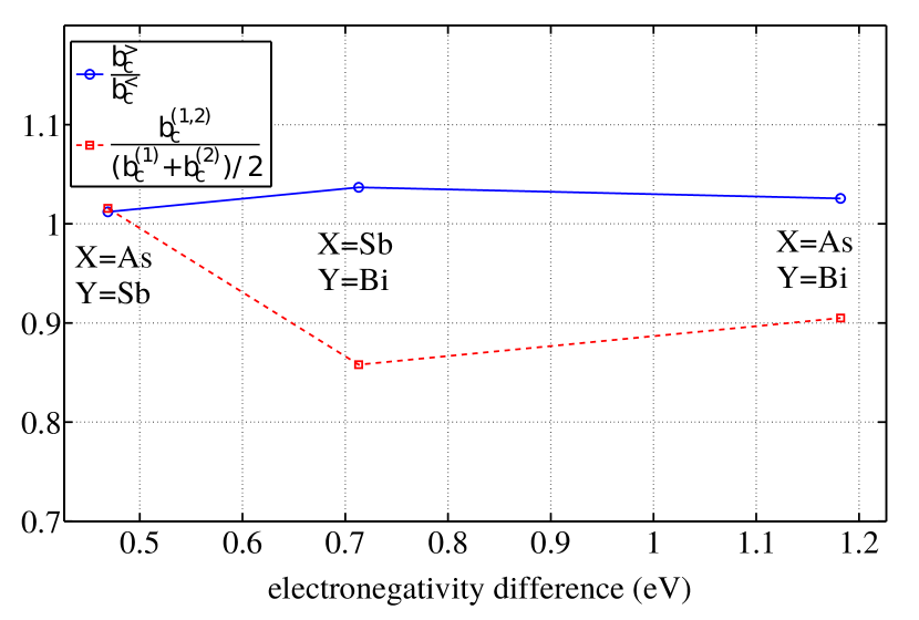
Figure S6: Critical lengths for the heteronuclear 3/4 trimers XH₂-YH₁-XH₂ and YH₂-XH₁-YH₂ from Fig. S5. $b_{c}^{>}$ and $b_{c}^{<}$ correspond to the situation where the more electronegative element (X) is placed in the central and terminal position, respectively. $b_{c}^{1}$ and $b_{c}^{1}$ denote the critical lengths for the homonuclear trimer XH₂-XH₁-XH₂ or YH₂-YH₁-YH₂.

VI Example of the Landau-Ginzburg free energy near a 1st order transition

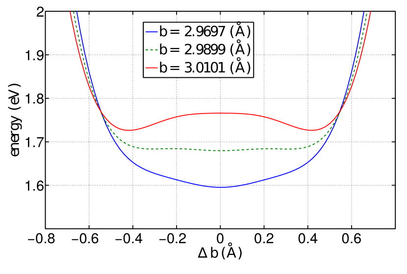
Figure S7: Slices of the full energy surface at $b=\text{const}$, for three values of the latter, for the 3/4 heterotrimer TeH-Sb-TeH near the symmetry breaking transition. The three distinct minima are present in one slice but are very shallow; the corresponding barriers would be easily erased by already zero-point vibrations.

VII Re-parametrization of antimony in MOPAC

MOPAC evaluates the matrix elements of the Hamiltonian using a approximation, in which their coordinate dependence is fully determined by coordinate dependence of the overlaps of the corresponding (atomic) basis orbitals. (WolfsbergHelmholz) Figs. S8-S11 show the wavefunction overlaps involving the pseudo-antimony with itself and with arsenic, and, for comparison, with MOPAC’s built-in As-As overlaps. MOPAC uses Slater-type orbitals. The lengthscale $\xi$ refers to the orbital exponent that determines the inverse rate of the exponential decay of the wavefunction overlap.

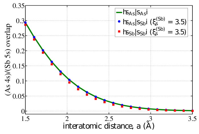
Figure S8: The $s$ wavefunction overlaps as functions of separation for As-As, As-Sb and Sb-Sb bonds.

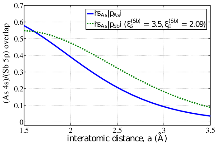
Figure S9: The $sp$ wavefunction overlaps as functions of separation for As-As and As-Sb bonds.

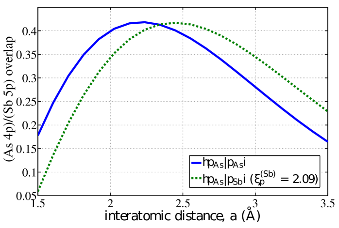
Figure S10: The $pp$ wavefunction overlaps as functions of separation for As-As and As-Sb bonds.

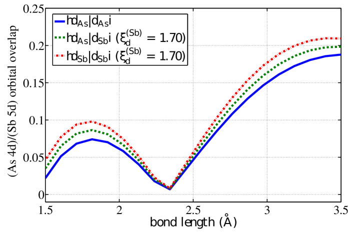
Figure S11: The $dd$ wavefunction overlaps as functions of separation for As-As, As-Sb and Sb-Sb bonds.

VIII Re-parametrization of MOPAC PM6 basis set under pressure

MOPAC employs one, Slater-type wave function per atomic orbital with a fixed extent. The latter is optimized to match geometries and formation enthalpies at normal conditions. Such a single-wavefunction parametrization may not be quantitative at high pressures, however. To test for this potential complication, we have solved for the HF wavefunctions of the 3/4, homonuclear arsenic trimer using a Quantum Chemistry package that approximates atomic wavefunctions with a linear combination of five Gaussian type functions (GTF); the widths of the individual Gaussians span a substantial range. We then monitor the coefficients at individual GTF’s as functions of density.

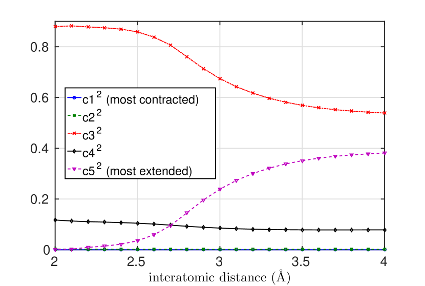
Figure S12: Composition of the $p$ atomic orbital in $pp\sigma$ bonding MO in arsenic trimer as a function of interatomic separation, from ORCA aug-cc-pvtz all electron HF calculations.

Fig. S12 shows the makeup of a $p_{z}$ atomic orbital in the $pp\sigma$ bond as a function of the As-As bond length. The vertical axis shows the square of coefficients $c_{1}$-$c_{5}$, 1 representing the least extended and 5 representing the most extended Gaussian function. As the ion cores approach each other, the wavefunction becomes less diffuse; $c_{3}$ grows while $c_{5}$ shrinks.

In addition, MOPAC’s default parametrization of the hard core repulsion between the ionic cores may not be fully adequate in the broad density range of interest. (Within the MOPAC PM6 method, the Pauli repulsion between closed shells is approximated with Voityuk’s diatomic expression(VR104).)

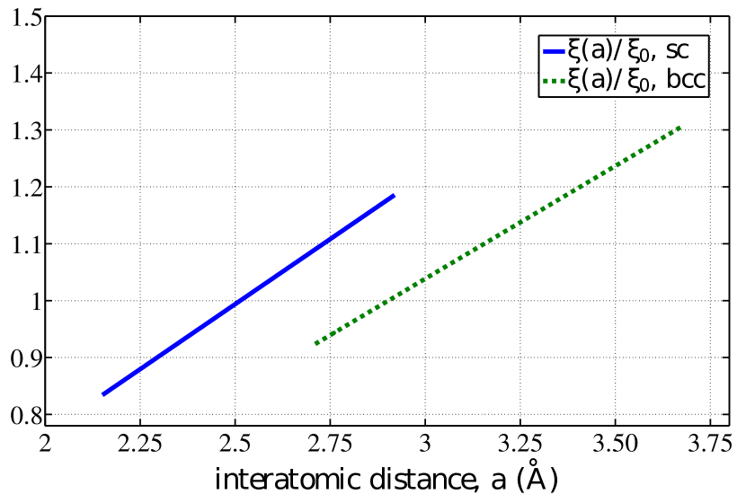
Figure S13: Orbital exponent scaling function behavior for simple cubic and body centered cubic lattices, illustrated using the ratio of the scaled exponent $\xi(a)$ to the default PM6 value $\xi_{0}$

The above notions are consistent with our findings that MOPAC’s built-in parametrization does not correctly locate the transition densities for the sc-to-bcc transition in elemental arsenic (sc=’simple cubic’, bcc=’body-centered cubic’). As a stopgap solution, we have introduced additional parametrization to both the orbital exponent $\xi$ of the wavefunction overlap and the parameter $\chi$ which is the overall scaling factor for the core-core repulsion. The resulting parametrization of $\xi$ and $\chi$ as functions of the lattice constant $a$ is shown in Figs. S13 and S14, respectively. Using the common tangent method, Fig. S15, we confirm a first order simple cubic to body centered cubic transition at 97 GPa and the experimental volume fraction $V_{T}/V_{0}$ reported in high pressure xray crystallography studies. The equation of state for bcc-As can be found in Ref. (PhysRevB.51.597) Note there is a coexistence region between the simple cubic and bcc phases where the structure is thought to be incommensurate. (PhysRevB.77.024109) In the absence of information on the pressure dependence of the density within the inter-transition region, we use a simple linear form of the scaling functions in that region. By the same token, the above re-parametrization is consistent with a continuous transition between rhombohedral and simple cubic at 25 Gpa, while the experimental $V_{T}/V_{0}$ is also recovered. (PhysRevB.41.5535)

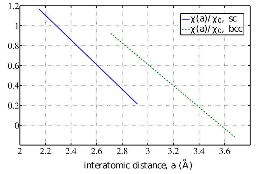
Figure S14: Linear core-core repulsion pseudo-potential scaling functions for simple cubic and body centered cubic lattices.

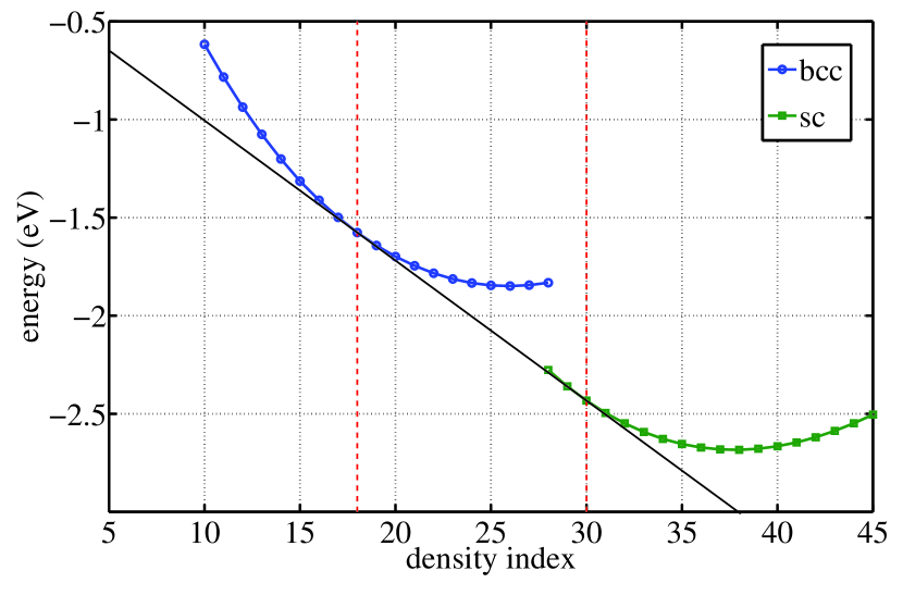
Figure S15: Common tangent construction of the first order simple cubic to bcc phase transition for the pseudo-arsenic material at $\epsilon$ = 0. The density index shown on the horizontal axis is an internal variable used in the PM6 calculations to set a common density in both the simple cubic and bcc lattices, the values of $18$ and $30$ marked with vertical dashed lines correspond to the experimentally observed boundaries of the first order transition.

IX Hysteretic behavior of the energy as a function of the electronegativity variation

We have found that the self-consistent Hartree Fock procedure does not always converge to the variational bound on the true ground state that is actually accessible to MOPAC. Given this uncertainty, we have performed many $\epsilon$ “sweeps,” whereby the electronegativity differential $2\epsilon$ is cycled between values of 0 and 8 eV. The result of this protocol is exemplified in Fig. S16. The cycling was terminated when two consecutive sweeps back and forth did not produce a jump to a lower yet term.

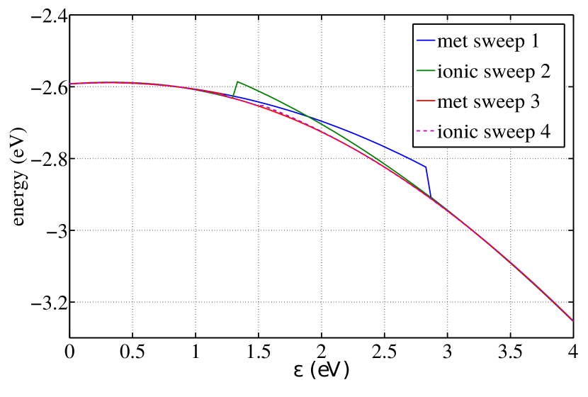
Figure S16: A sample of the “sweep” protocol demonstrating an overshoot of a term crossing. Labels “met” and “ionic” correspond with sweeps that begin at the $\epsilon=0$ and $\epsilon=4$ eV ends of the $\epsilon$ range.

X Stability of the simple cubic structure to rhombohedral distortion

Fig. S17 shows the energy of a 64 atom pseudo-arsenic solid as a function of the magnitude of a distortion toward the rhombohedral lattice, as in Fig. 12 of the main text. Hereby, we shift the anionic and cationic sublattice relative to each other along the [111] direction. At the higher of the two densities shown in Fig. S17, the presence of a central minimum indicates that the distortion is destabilizing. This is approximately the density where the rhombohedral-to-simple cubic transition is observed experimentally. (PhysRevB.41.5535)

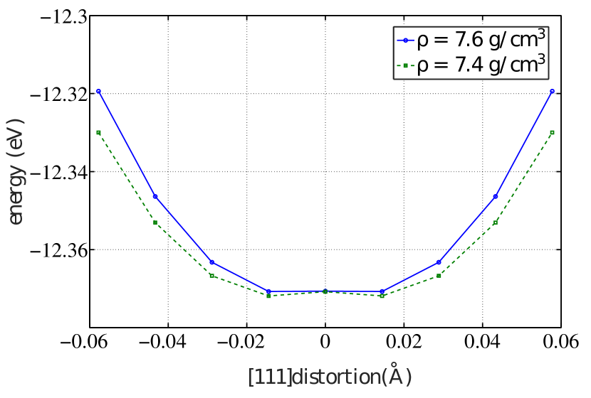
Figure S17: Onset of susceptibility to small distortion towards rhombohedral structure, as probed by relative shift of the cationic and anionic sublattices comprising the rock-salt structure of the pseudo di-pnictogen compound.

XI Decrease in $sp$-mixing in rhombohedral arsenic with density

To examine $sp$-mixing in rhombohedral arsenic we have used the projected crystal orbital Hamilton population (pCOHP) analysis tool Lobster (doi:10.1021/j100135a014; doi:10.1021/jp202489s; JCC:JCC23424) to extract chemical bonding information from the results of plane-wave calculations. pCOHP is a close relative of the crystal orbital overlap population (COOP) analysis, originally known as overlap population density of states (OPDOS).

Density functional theory (DFT) calculations were performed in the generalized gradient approximation (GGA) parameterization of Perdew, Burke and Emzerhof (PBE38; CA45) using the Vienna ab-initio Simulation Package (VASP) version 5.3 (PhysRevB.47.558; KRESSE199615; PhysRevB.59.1758) with Blochl’s projector augmented-wave (PAW) method employed for the core states. (PEB50) In the rhombohedral structure at ambient pressure, there is a gap between the $s$ and $p$ contributions to the overall density of bonding states, as shown in Fig. S18.

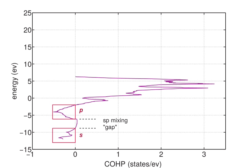
Figure S18: The dashed line indicate a gap between portions of the electronic density of states primarily associated with bonding $s$ and $p$ electrons, in rhombohedral arsenic at normal conditions. The red boxes show $s$ and $p$ contributions to the density of bonding states.

We next compress the unit cell while simultaneously reducing the rhombohedral distortion until we reach the density where the phase transition to simple cubic is observed experimentally. The width of the gap region shown in Fig.S18 shrinks with density before vanishing at the transition. We interpret this shrinking as a decreased mixing between the $s$ and $p$ bonding sub-systems.

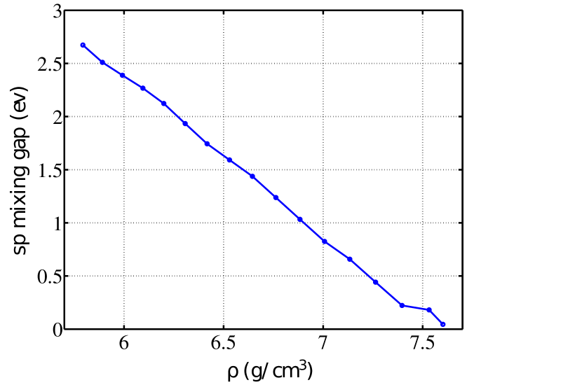
Figure S19: The dependence of the $sp$ from Fig. S18 as the sample is compressed and deformed toward the simple cubic structure.

XII Ab-initio verification of electronic symmetry breaking for symmetric AsH₂-AsH-AsH₂ trimer

To verify the apparent change in the bond characteristics, as implied by the MOPAC-based, LMO analysis, we have obtained variational HF solutions for the symmetric 3/4 trimer AsH₂-AsH-AsH₂ using the 6-311G basis within Gaussian 09.(g09) The latter Quantum Chemistry package provides an alternative interpretational tool to analyse bonding, viz., via the NBO 6.0 Natural Bond Orbital (NBO). (NBO6) Natural Bond Orbitals (NBOs) are an orthonormal set of localized orbitals in the form of core orbitals (CR) bonding orbitals (BD), lone pairs (LP) and multi-center orbitals (nC). The first three orbital types are Lewis-type orbitals. The procedure attempts to maximize the occupancy of these Lewis orbitals, the remaining electronic density assigned to non-Lewis, multi-center orbitals.

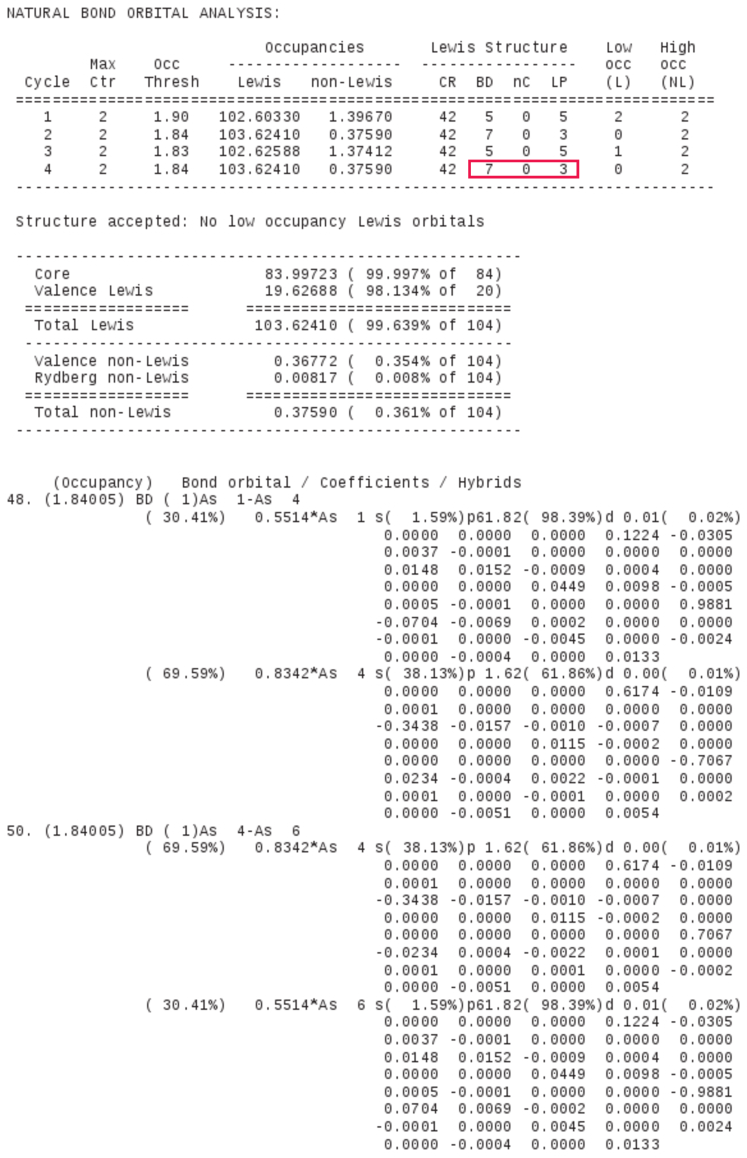
Figure S20: Fragment of the output of the NBO6 analysis within Gaussian09 for spatially-symmetric trimer at $b=3.2$ Å.

Similarly to the LMO-based conclusions in the main text, we have detected a qualitative change in the NBOs by which a three-center orbital and associated lone pair emerge for sufficiently long trimers. Fragments of the corresponding output files just before and after the transition are provided in Figs. S20 and S21, respectively. For the reader’s convenience, we framed the results of the final iteration of the NBO procedure, which indicate that following the transition, the number of two-center bonds decreased by 2 while a three-center bond and a lone pair appeared. See also the framed entry in Fig. S21 for orbital 52. The configurations in Figs. S20 and S21 correspond to the As-As bond lengths $b=3.2$ and $3.3$ Å, respectively, which is less than but reasonably close to MOPAC’s figure $b\approx 3.6$ Å. Importantly, this figure is still much longer than what is expected for the covalent As-As bond, i.e., 2.4 Å or so.

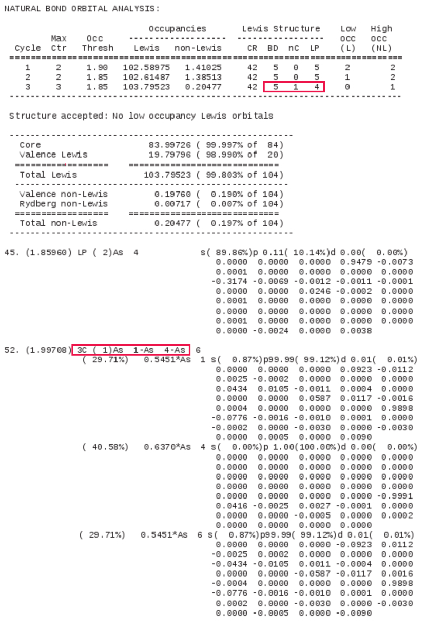
Figure S21: Fragment of the output of the NBO6 analysis within Gaussian09 for spatially-symmetric trimer at $b=3.3$ Å.

XIII Walsh diagram of the molecular terms of the trimer AsH₂-AsH-AsH₂ as functions of the trimer length

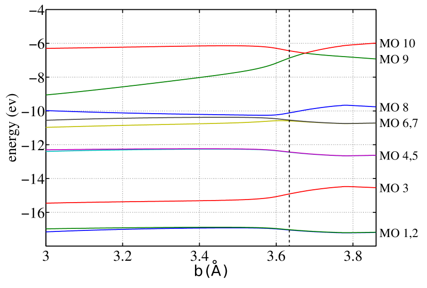
Figure S22: MOPAC-derived molecular orbital terms for the AsH₂-AsH-AsH₂ trimer as functions of the As-As bond length $b$. The vertical dashed line indicates the bond length at which the LMO transition takes place.

XIV Bonding from the viewpoint of localized molecular orbitals

We will characterize bonding using the localized molecular orbital (LMO) formalism. Originally inspired by symmetry adapted orbitals in relatively symmetric molecules, the localized molecular orbitals can be assigned for arbitrary geometries: Given a set of occupied molecular orbitals $\psi_{i}$, one transforms to an alternative set of orthonormal orbitals $\chi_{j}$ such that a certain quantity reflecting the self-repulsion within individual new orbitals is maximized.(SB32; ER35; VN56; PS78) Specifically, here we adhere to the Edmiston and Ruedenberg approach (ER35), whereby one maximizes the quantity $D_{\chi}\equiv\sum_{j}\int d^{3}\bm{r}_{1}d^{3}\bm{r}_{2}|\chi_{j}(\bm{r}_{1})|^{2}V(r_{12})|\chi_{j}(\bm{r}_{2})|^{2}$ or, equivalently, minimizes the mutual repulsion among distinct orbitals in the form of the quantity: $\sum_{j<k}\int d^{3}\bm{r}_{1}d^{3}\bm{r}_{2}|\chi_{j}(\bm{r}_{1})|^{2}V(r_{12})|\chi_{k}(\bm{r}_{2})|^{2}$. The function $V(r_{12})$ stands for a purely repulsive potential energy function. The LMOs are generally not eigenfunctions of an effective one-particle Hamiltonian, such as that arising in the Hartree-Fock (HF) approximation. Instead, they represent an attempt by an interpreter to redistribute (the already bound) electrons among orthonormal, maximally localized orbitals, each of which thus binds together the smallest number of atoms. The latter number serves as a lower bound on the number of centers in a bond; the bound is not unique because it depends on the specific choice of the test function $V(r_{12})$, which is made according to one’s convenience and computational means. For instance, $V(r_{12})=r_{12}^{-1}$ implies localization with respect to (non-screened) Coulomb repulsion. A more computationally convenient choice is $V(r_{12})=\delta(\bm{r}_{12})$, which simply yields $D_{\chi}=\sum_{j}\int d^{3}\bm{r}|\chi_{j}(\bm{r})|^{4}$.

The above procedure is significantly simplified when the one-electron energy function is diagonalized while neglecting the overlap between distinct atomic orbitals, as is the case for certain semi-empirical approximations. (PS78) Hereby, one can present the integral $\int d^{3}\bm{r}|\chi_{j}(\bm{r})|^{4}$ as a sum over distinct atoms: $\sum_{A}\int_{A}d^{3}\bm{r}|\chi_{j}(\bm{r})|^{4}$, where the individual integrations are over regions occupied by distinct atoms. Each such integration yields a quantity that scales inversely proportionally with the atom’s volume. Insofar as we are interested in the partitioning of the electrons between atoms, irrespective of the extent of the atomic orbitals, the above sum can be profitably replaced by a (dimensionless) expression, viz.:

$$\int d^{3}\bm{r}|\chi_{n}(\bm{r})|^{4} =\sum_{A}\int_{A}d^{3}\bm{r}|\chi_{n}(\bm{r})|^{4}\to$$ (S2)

$$n_{j} \equiv\sum_{A}\left(\sum_{\lambda_{A}}C^{2}_{\lambda_{A}j}\right)^{2},$$ (S3)

where we have expanded the localized orbital $\chi_{j}(\bm{r})$ in terms of the atomic orbitals $\phi_{\lambda_{A}}$:

$$\chi_{j}(\bm{r})=\sum_{A}\sum_{\lambda_{A}}C_{\lambda_{A}j}\phi_{\lambda_{A}}$$ (S4)

and the index $\lambda_{A}$ labels the atomic orbitals on atom $A$. As already mentioned, $\int dV\phi_{\lambda}\phi_{\mu}=\delta_{\lambda\mu}$, implying $\sum_{A}\sum_{\lambda_{A}}C^{2}_{\lambda_{A}n}=1$. The quantity $n_{j}$ from Eq. (S3) clearly provides the participation number of distinct centers to the localized orbital $j$, and is appropriately called the bond-center number. (PS78) For a lone pair, one automatically gets $n=1$. For a two-center bond, the MO and LMO are equal: $\chi=\psi=\alpha\phi_{1}+\beta\phi_{2}$, ($\alpha^{2}+\beta^{2}=1)$; the bond center number, $n=[\alpha^{-4}+(1-\alpha^{2})^{-2}]^{-1}$, is maximized at 2 for a covalent bond, $\alpha=1/\sqrt{2}$, and is minimized at the lone pair value 1 for a purely ionic bond, $\alpha=0,1$. For a linear trimer with two equivalent bonds and one orbital per center, one may use the Hückel energy function:

$$\widehat{H}=-\left({\begin{array}[]{*{20}{c}}0&\beta&0\\ \beta&0&\beta\\ 0&\beta&0\end{array}}\right).$$ (S5)

The corresponding MO’s are shown graphically in Fig. S23(a). The lowest-energy MO is $\psi_{1}=\phi_{1}/2+\phi_{2}/\sqrt{2}+\phi_{3}/2$ and the (formally) non-bonding MO is $\psi_{2}=(\phi_{1}-\phi_{3})/\sqrt{2}$. If only the ground state MO contributes to bonding, one gets $n=8/3$. This value is less than three, in reflection of the non-uniform distribution of charge among the three centers, viz., $25\%$, $50\%$, and $25\%$ respectively. The partially ionic character of the three-center bond for a linear trimer made of otherwise equivalent atoms was noted a while ago by Musher. (MusherAngew1969) (For comparison, the bond-center number for a three-center bond with three equivalent centers, $\chi=\psi=(\phi_{1}+\phi_{2}+\phi_{3})\sqrt{3}$ exactly equals $3$.) In the case when MO2 is actually bonding, there are two LMOs. Direct computation shows $\chi_{1,2}=(\psi_{1}\pm\psi_{2})/\sqrt{2}$, the two shown graphically in Fig. S23(b). The two LMOs are equivalent in that they are mirror images of each other, up to the sign, and each can be associated with a one-electron energy $(E_{1}+E_{2})/2$. (Generally, to the $j$-th LMO $\chi_{j}=\sum_{l}c_{jl}\psi_{l}$, one may associate an energy $E_{j}=\sum_{l}c_{jl}^{2}E_{l}$, where the summations are over the occupied MOs.) The bond number for each of the two LMOs is $n_{1,2}=32/19$, which is just short of 2. This (modest) deficit is, again, due to the non-uniform distribution of charge among the three centers. Still, insofar as the bond-center numbers for the two LMOs are numerically close to 2, the 3 center/4 electron bond can be thought of as two adjacent two-center bonds.

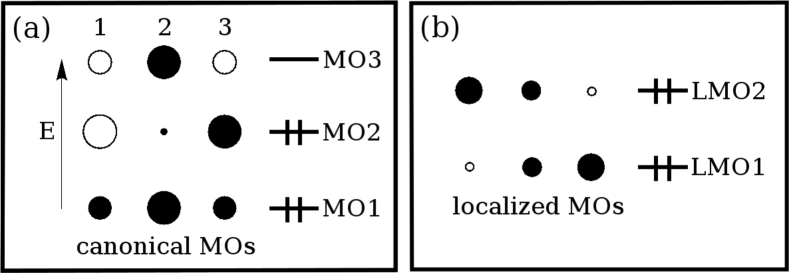
Figure S23: (a) Graphical representation of the eigenvectors of the three-orbital, Hückel energy function (S5). (b) The localized molecular orbitals (LMOs) corresponding with panel (a). Note the two orbitals have the same energy, $(E_{1}+E_{2})/2$.

A useful pattern emerges from the above trimer example already at the Hückel level, as in Fig. S23: If the two-center bonds comprising the three-center bond are equivalent and the two bonding molecular orbitals have opposite parity, the two resulting LMOs are necessarily mirror images of each other. (This pattern does not necessarily hold when the number of MOs exceeds two, whether that number is even or odd.) If only one LMO is present, on the other hand, it must be either odd or even with respect to reflection in the symmetry plane.

As a measure of the bond order for a two-center bond connecting atoms A and B, one may evaluate the number of electrons shared by these atoms according to: (APS627)

$$B_{AB}\equiv\sum_{\lambda_{A}\!,\,\lambda_{B}}P^{2}_{\lambda_{A}\lambda_{B}},$$ (S6)

where $P_{\lambda\mu}$ is the density matrix:

$$P_{\lambda\mu}\equiv 2\sum_{i}\widetilde{C}_{\lambda i}\widetilde{C}_{\mu i},$$ (S7)

the summation being over the occupied MOs, and the $\widetilde{C}$s are the expansion coefficients for the MOs in terms of the atomic orbitals:

$$\psi_{i}(\bm{r})=\sum_{A}\sum_{\lambda_{A}}\widetilde{C}_{\lambda_{A}i}\phi_{\lambda_{A}}.$$ (S8)

The quantity in Eq. (S6) is often called the “Wiberg bond index.”(APS627) For a lone pair, $B=0$ automatically. For a two-center bond, $\psi=\alpha\phi_{1}+\beta\phi_{2}$, $B_{AB}=4\alpha^{2}(1-\alpha^{2})$; it varies between 0 and 1, the two extremes corresponding to a purely ionic and covalent bond, respectively. For the trimer from Eq. (S5), the bond orders are $B_{12}=B_{12}=1/2$, and $B_{13}=1/4$, whether the number of the bonding MO’s is one or two. We thus conclude that the bond order defined in Eq. (S6) reflects, to some extent, the deviation of the bonding in Fig. S23 from a collection of two-center bonds, since $1/2+1/2+1/4=1.25>1$.

To gain additional insight, one may quantify the bonding contribution of an individual LMO, $j$, by evaluating the expectation value of the density matrix for the orbital, see “Localization Theory” in the online MOPAC Manual (MOPACmanual)

$$C^{\text{(bond)}}_{jj}\equiv\left\langle\chi_{j}|\widehat{P}|\chi_{j}\right\rangle=2\sum_{\lambda\mu}C_{\lambda j}C_{\mu j}P_{\lambda\mu},$$ (S9)

where in the sum above, terms pertaining to the same atom are excluded. The bonding contribution for a lone pair is automatically $0$. For a two-center bond $\chi=\psi=\alpha\phi_{1}+\beta\phi_{2}$, $C^{\text{(bond)}}=8\alpha^{2}(1-\alpha^{2})$, which is simply the Wiberg bond index times two. Likewise, the trimer from Eq. (S5) in the one-LMO arrangement yields $C^{\text{(bond)}}=2.5$. The two-LMO arrangement leads to $C^{\text{(bond)}}_{11}=C^{\text{(bond)}}_{22}=1.25$, so that the total bond contribution is, again, $2.5$. Thus based on the bond index and bond contribution analysis, the bond order for the Hückel trimer is not sensitive to whether MO2 is regarded as bonding or non-bonding. We shall see that the two analyses give different results in more complicated situations.

XV The eventual dissociation of the trimer, from the LMO perspective

XVI A realization of a 5-center localized molecular orbital

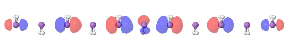
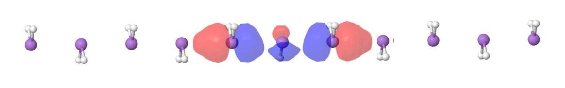
Figure S25: MOPAC-derived $pp\sigma$ molecular orbital (top) and corresponding localized molecular orbital (bottom). All nearest neighbor As-As bond lengths are equal to $3.39$ Å. The hydrogens are constrained in the same fashion as for the 3/4 trimer in the main text.

XVII The 20-member ring hosts a charge-density wave (CDW)

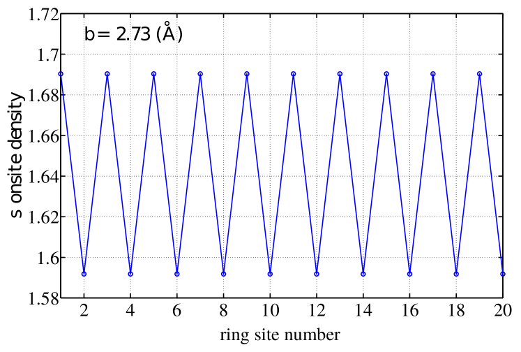
Figure S26: An example of a charge density wave in the 20-member ring (AsH₂)₂₀, as inferred from the diagonal entries of the density matrix, see main text. The specific bond length, $b=2.73$ Å, corresponds with the ground state configuration of the non-dimerized 20 member ring at the ground state configuration indicated by the asterisk in Fig. 14 of main text.

XVIII The 20-member ring becomes unstable toward dimerization for bond lengths exceeding 2.5 Å

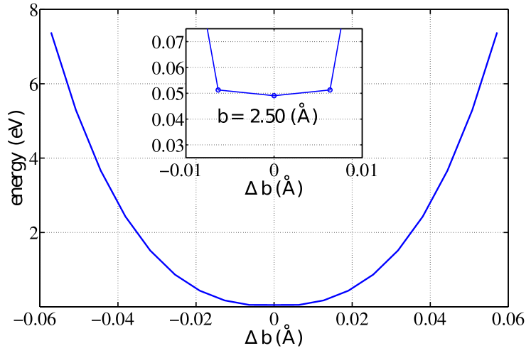
Figure S27: Electronic energy of the 20-member ring (AsH₂)₂₀ as a function of the dimerization strength. The latter is indicated by the length difference between the longer and shorter bond. The average bond length is kept steady at $2.50$ Å.

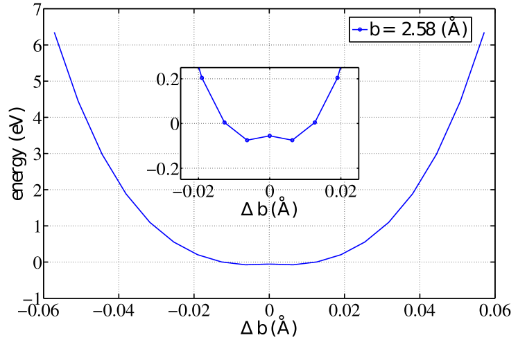
Figure S28: Electronic energy of the 20-member ring (AsH₂)₂₀ as a function of the dimerization strength. The latter is indicated by the length difference between the longer and shorter bond. The average bond length is kept steady at $2.58$ Å.

XIX Additional examples of localized molecular orbitals near the ground state length of the non-dimerized 20-member ring

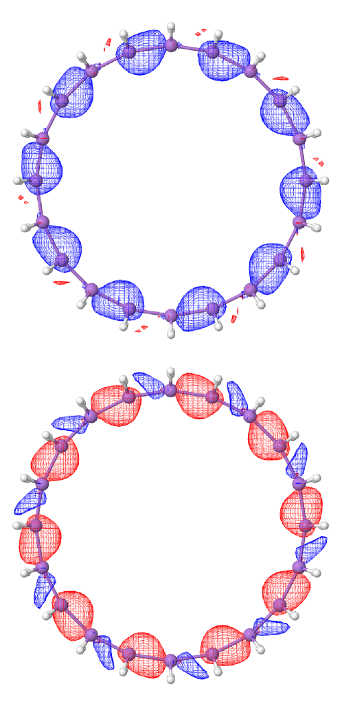
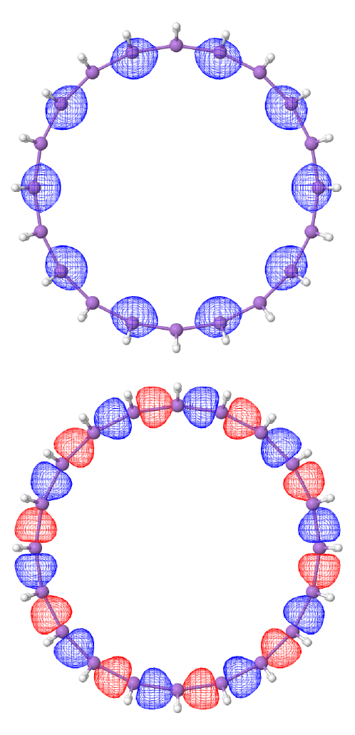
Figure S29: Left: The LMOs near the mechanical stability limit of the 20-member ring (AsH₂), a higher energy HF solution than the one visualized in Fig. 13 of main text, regime III; $b=2.58$ Å. Right: The LMOs for the ground state configuration of the non-dimerized 20 member ring at the ground state configuration indicated by the asterisk in Fig. 14 of main text.

XX Molecular geometry for the $AsH_{2}-AsH-AsH_{2}$ and $AsH_{2}-AsH_{2}-AsH_{2}$ trimers

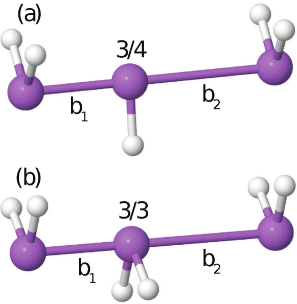
Figure S30: The trimers AsH₂-AsH-AsH₂ (panel (a)) and AsH₂-AsH₂-AsH₂ (panel (b)), corresponding to 3-center/4-electron and 3-center/3-electron $pp\sigma$ bond.

XXI Spatial symmetry breaking in the $AsH_{2}-AsH-AsH_{2}$ trimer

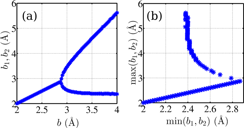
Figure S31: The equilibrium values of the As-As bond lengths for a fixed value of the overall trimer length, according to the dashed line on the associated potential energy surface in the main text; (a) as functions of the trimer length per bond, (b) plotted parametrically, for the longer bond vs. the shorter bond.

XXII Term crossing upstream of the LMO transition in the $AsH_{2}-AsH-AsH_{2}$ trimer

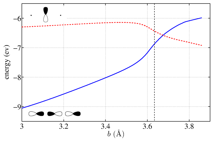
Figure S32: The energies of the MOs responsible for the $pp\sigma$ bond and the lone pair on the central arsenic, as functions of the As-As bond length $b=b_{1}=b_{2}$, for the 3/4 case. The vertical dashed line indicates the location of the LMO transition in Fig. 13 of the main text.

XXIII Potential energy of the $AsH_{2}-AsH-AsH_{2}$ trimer

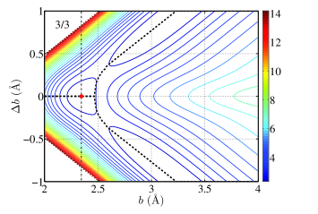
Figure S33: The contour plot of the potential energy of the 3/3 trimer, Fig. S30(a), as a function of the trimer length per bond $b\equiv(b_{1}+b_{2})/2$ and the distance of the center arsenic from the midpoint between the terminal arsenics, $\Delta\equiv(b_{1}-b_{2})/2$. The metastable symmetric configuration is marked by the filled red circle. The dashed, bifurcating graph shows the minimum energy at fixed value of $b$.

XXIV Localized molecular orbital analysis of the 3 electron multi-center bond

Figure S34: The bonding contribution of the LMOs as functions of the As-As bond length $b=b_{1}=b_{2}$, for the 3/3 molecule.

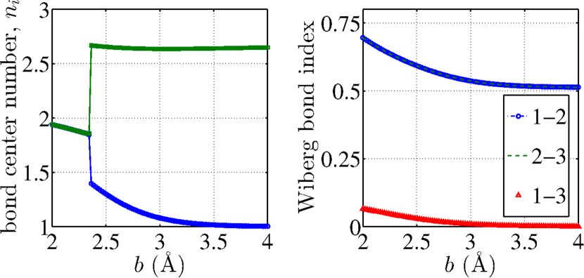
Figure S35: Displayed as functions of the As-As bond length $b=b_{1}=b_{2}$: (a), the bond center number for the LMOs from Fig. S34; (b), the Wiber bond index. Note the latter is computed using the density matrix and does not rely on the localization procedure.

XXV Bond evolution in the $(AsH_{2})_{20}$ ring molecule

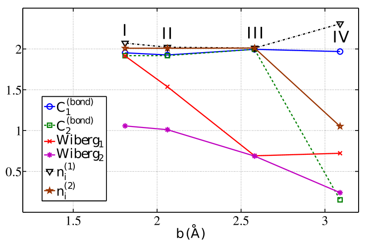
Figure S36: The values the bonding contribution, Wiberg bond number, and the center number for the four configurations in Fig. 18 of the main text. The lines are guides to the eye.

XXVI AIM based analysis of bond evolution in symmetric $AsH_{2}-AsH-AsH_{2}$ trimer

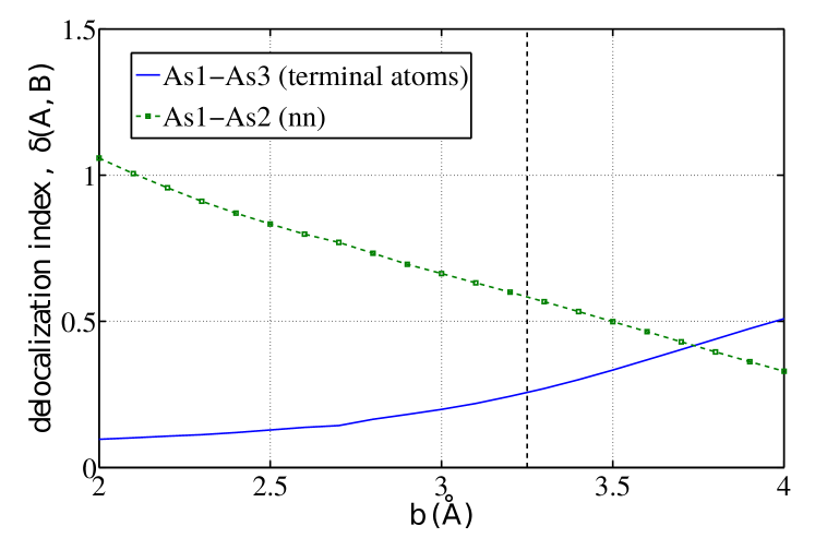
Figure S37: Evolution of the the delocalization indices for electron densities associated with nearest-neighbor and multi-center bonds in the 4-electron/3-center arsenic trimer.