An evolutionary strategy for $\Delta$E - E identification

Abstract

In this article we present an automatic method for charge and mass identification of charged nuclear fragments produced in heavy ion collisions at intermediate energies. The algorithm combines a generative model of $\Delta$E - E relation and a Covariance Matrix Adaptation Evolutionary Strategy (CMA-ES). The CMA-ES is a stochastic and derivative-free method employed to search parameter space of the model by means of a fitness function. The article describes details of the method along with results of an application on simulated labeled data.

particle identification methods, heavy-ion, detector, Pattern recognition, calibration, fitting, CMA-ES, covariance matrix adaptation, evolutionary strategy 1234.56789

1 Introduction

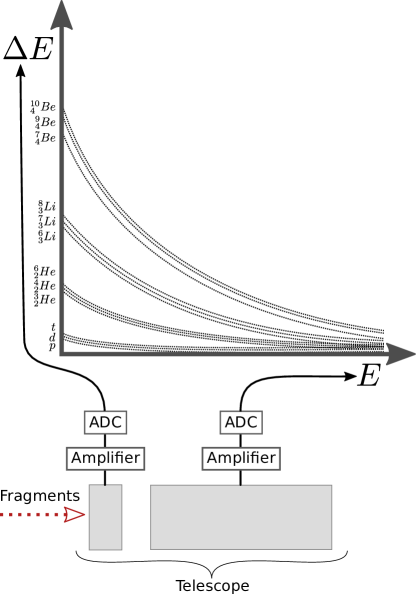
In heavy ion collisions at intermediate energies many fragments of different mass (A) and charge (Z) are produced due to multi-fragmentation processes. The number of those fragments is not constant and depends on many conditions: mass of target and projectile, impact parameter and the energy of the projectile. The fragments are often detected in telescopes, stacks of different thickness detectors, assembled in an array to cover the full solid angle. Such detection systems have been developed in many research institutes [1, 2, 3, 4, 5, 6, 7, 8]. The number of telescopes in such arrays vary from few hundreds [6] to over a thousand [5]. The measurements of fragment energy losses in each layer of the telescope are the key to the identification process. The correlation between the energy loss in one or several layers versus the residual energy released in the detector in which the particle has stopped, reveals specific curved lines, each representing a set of signals from fragments of the same A and Z (see fig. 1).

Figure 1: A schematic overview of $\Delta$E-E identification procedure. Different fragments produced in a nuclear reaction and stopped in a telescope, populate identification lines characteristic of their charge and mass.

The general performance of the detectors depends obviously on their quality and the associated electronics but also on the homogeneity of their response and their stability over long periods of time (e.g. temperature). Thus, each telescope can give a different $\Delta$E-E matrix, which can change during data-taking. In the end, the identification procedure has to be performed several times for each telescope before physics analysis can start.
Nowadays there are several methods used to determine mass and charge of detected fragments. In general, they can be grouped in several classes, however some parts of those methods may overlap.

1. Graphical - is the most trivial set of methods where an user draws interactively and by hand curves on the $\Delta$E-E matrix. Particles are then identified by comparing distances to the closest lines.

2. Fitting methods:

   1. Algorithms are used to find parameters of a function describing $\Delta$E-E correlation for a subset of ridges[9, 10, 11]. Particle identification is obtained by inversion of the function for given $\Delta$E and E, in order to extract Z and possibly A.

   2. Methods that calculate energy loss tables with the use of a priori knowledge about the incident ion (mass, charge and energy) and about the absorber medium (volumetric density and atomic number)  [12, 13, 8, 14]. Each particle is then identified from its relative distance between pairs of the closest ridge lines.

3. Peak finding methods:

   1. Methods built on top of one of the above methods, the lines need to be drawn by hand or fitted to the $\Delta$E-E matrix, which is followed by the linearization procedure [6]. After linearization, data is projected onto a one-dimensional plot producing quasi-Gaussian peaks. The isotopic peaks within an element are fitted with Gaussian functions that are then correlated to masses.

   2. A part of the matrix is projected onto a relevant helper line, D($\theta$), followed by a peak localization. The operation of projection/localization is then repeated in order to cover the full matrix, varying a helper line $\theta$ from $0$ to $90\degree$. [15]

The quality of the identification procedure in the first, graphical method is fully user dependent and extremely time consuming. It does not allow any extrapolation into the low statistics region, which is possible in other described methods. Fitting procedures are very sensitive to statistics and they usually require additional constraints provided by a user. For example in method described in 2(b) it is extremely important to know with good precision each $\Delta$E detector the active thickness and dead layer. The last mentioned method is the least user-intervention dependent (”only two mouse-clicks from the user to calculate all initialization parameters”), however the choice of the first click seems to be crucial for a final result. The histogram binning also has to be chosen carefully. The strength of the method is that it can be used to many types of 2 dimensional matrices, instead of only $\Delta$E-E correlations. Nevertheless, the common feature of all above methods is that they require a dedicated graphical interface. The method presented in this article is an adaptation of evolutionary algorithm for particle trajectory reconstruction [16]. It belongs to a class of fitting methods, however it provides great improvements. It does not require any user interaction, any initial parameters provided and also does not require a graphical interface. It requires only a file with the x and y positions of points being signals from the E and $\Delta$E detectors and a model, which describes the relation between those points. As the result of the algorithm, the file gains two more columns, which are Z and A assigned to each E and $\Delta$E pair. In the following sections, we describe the model used to interpret data as well as the data association and the classification algorithms. At the end, a test procedure is described and the results are presented together with short discussion on strong points as well as drawbacks.

2 The model

Correlations between measured energy losses in two successive detectors ($\Delta$E - E) create a specific pattern, presented on fig. 2, which can be easily modeled. In order to build a model, we have used the function proposed by L.Tassan-Got [10]. For detectors delivering a linear response (e.g. silicon detectors), it reads:

$$\Delta E=t(E,g,\mu,\lambda,A,Z)=\Bigg{[}(gE)^{\mu+1}+\Big{(}\lambda Z^{\frac{2}{\mu+1}}A^{\frac{\mu}{\mu+1}}\Big{)}^{\mu+1}\Bigg{]}^{\frac{1}{\mu+1}}-gE$$ (1)

where the parameters we are looking for are G, $\lambda$ and $\mu$. However it has already been noticed in the past [9, 17] that for a wider Z range, the above formula must be extended by additional parameters $\alpha$, $\beta$, $\nu$ and $\xi$:

$$\Delta E=t(E,g,\mu,\nu,\lambda,\alpha,\beta,\xi,A,Z)=\Bigg{[}(gE)^{\mu+\nu+1}+\Big{(}\lambda Z^{\alpha}A^{\beta}\Big{)}^{\mu+\nu+1}+\xi Z^{2}A^{\mu}(gE)^{\nu}\Bigg{]}^{\frac{1}{\mu+\nu+1}}-gE$$ (2)

For a detector delivering a non linear response versus deposited energy this function needs to be corrected. The energy E in equation 2 must now be expressed as a function of the light h emitted by the scintillator. The light response of CsI(Tl) crystals is deduced from the Birks formula [18] and allows expression of the energy released in the CsI as a function of the emitted light :

$$E=\sqrt{h^{2}+2\rho h\Bigg{[}1+\ln{\big{(}1+\frac{h}{\rho}\big{)}}\Bigg{]}}$$ (3)

where $\rho=\eta Z^{2}A$ is a new parameter.
In our method we have used the function for linear detectors (1) to build our model in the following manner:

$$\mathrm{model}\quad\begin{cases}t(E,g,\mu,\lambda,A_{1},Z_{1})\\ \dots\\ t(E,g,\mu,\lambda,A_{n},Z_{n})\\ \end{cases}\quad\mathrm{where}\quad\{A_{i},Z_{i}\}\in I$$ (4)

The set $I$ contains mass number (A) and atomic number (Z) pairs for isotopes of interest, in the presented model from ${}^{1}_{1}$H up to ${}^{25}_{12}$Mg. The model is easily adjustable with regards to the type of fragments by manipulating the parameters $A$ and $Z$. When model is ready, the next step is to interpret the data. In the following section, we describe the data to model association algorithm as well as the method used to search the model parameter space.

3 Data classification

The algorithm is based on a generative model of $\Delta$E - E correlation. The model is iteratively compared with input data by means of a user defined fitness function. The function compares data and the model (eq. 4) with given parameters in order to evaluate the correctness of model parameters. In the evolutionary strategy the definition of a fitness function is a key point. We define it as follows:

$$f(D_{m,2}\,,g,\mu,\lambda)=\sum_{j=1}^{m}\underset{i\in I}{\operatorname{arg}\,\operatorname{min}}\;(D_{j,1}-t(D_{j,2}\,,g,\mu,\lambda,A_{i},Z_{i}))^{2}$$ (5)

where

$$D_{m,2}=\begin{bmatrix}\Delta E_{1}&E_{1}\\ \dots&\dots\\ \Delta E_{m}&E_{m}\\ \end{bmatrix}$$ (6)

denotes a matrix of $m$ input data points ($\Delta E$ and $E$ of fragments). In other words, the fitness function $f(\dots)$ quantifies minimal residual between every data point $p_{j}=[D_{j,1},D_{j,2}]$ and its closest function $t(\dots,A_{i},Z_{i})$ of the model.

With the model and fitness functions defined, the parameters $g$, $\mu$, $\lambda$ have to be estimated. In order to search the model parameter space, we have employed a method called Covariance Matrix Adaptation Evolutionary Strategy (CMA-ES) [19, 20, 21, 22].

The CMA-ES is an iterative, stochastic and derivative-free method designed for difficult non-linear, non-convex, black-box optimization problems in the continuous domain. This method is considered as state-of-the-art in evolutionary computation and it is typically applied to unconstrained optimization problems with search space dimensions between three and a hundred. The CMA-ES is an alternative for quasi-Newton methods such as very popular Broyden-Fletcher-Goldfarb-Shanno (BFGS) algorithm, in cases where derivatives are not available.

We have implemented the method using the R language[23] and C++ CMA-ES library[24] integrated by means of Rcpp package[25]. The decision to choose C++ implementation of CMA-ES has been made based on execution speed (it supports multi-threading) as well as due to advanced development stage of the project. The library is released under the GPLv3 license and offers rich set of options such as possibility to define basic CMA-ES parameters (e.g. $\mu$, $\lambda$), model parameter range bounds, gradient function, various top criteria, variation of CMA-ES method and more.

In the CMA Evolution Strategy, a population of new search point is generated by sampling a multivariate normal distribution $\mathbb{R}^{n}$. Those points are evaluated using a fitness function in order to select the best fit candidates. Afterwards, a new weighted mean is calculated based on selected candidates. The covariance matrix is adjusted accordingly in order to update the space search region for next iteration. The method described in this article uses a variation of CMA-ES called Active-CMA-ES[26], or in short, aCMA-ES . It differs from the regular one by selecting not only the best candidates but also the worst ones. The latter are used to adapt a covariance matrix faster towards minimum value of objective function. The aCMA-ES has proven to outperform classical variations of the algorithm[27].

After the aCMA-ES algorithm finds the minimum of objective function, the model parameters are used to classify the data. The classification is performed based on distance

$$d=|D_{j,1}-t(D_{j,2}\,,g,\mu,\lambda,A_{i},Z_{i})|$$ (7)

between a data point $p_{j}$ and a function $t(\dots,A_{i},Z_{i})$ of the model. For example, if a value of the function $t(E_{j},\dots,A_{25},Z_{12})$ is the closest to a data point $p_{j}$, then the point $p_{j}$ is classified as ${}^{25}_{12}$Mg.

In the following section, we present the performance of the working algorithm on simulated data with superimposed Gaussian noise.

4 Results

In order to test the algorithm, labeled data has been simulated with superimposed Gaussian noise as presented on the left panel of fig. 2. The numbers of particular isotopes (230k in total) have been based on real telescope from the NIMROD array [6]. The data was generated using set of functions described by eq. 4, which define our generative model.

Figure 2: Left: $\Delta$E - E points simulated using eq. 1 with Gaussian noise. Numbers of particular isotopes have been based on real telescope from NIMROD array. Right: Identification discrepancies of particular fragments after noise application. Negative values indicate number of fragments that have been underestimated, whereas positive indicate that they have been overestimated.

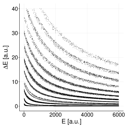
The parameters of the model g, $\mu$ and $\lambda$ were 0.25, 0.7 and 84, respectively. As a first step, the re-classification of data to lines generated with these parameters was performed. Due to a noise application, some of the $\Delta$E - E points have changed their position with respect to the original one so strongly, that their mass classification failed for 501 (0.22$\%$) fragments with Z ¿ 4. This means, that if our evolutionary algorithm reconstructed the model function parameters with 100$\%$ accuracy, 501 fragments would be in any case not correctly classified in mass number. The atomic number has been assigned correctly to all studied fragments. 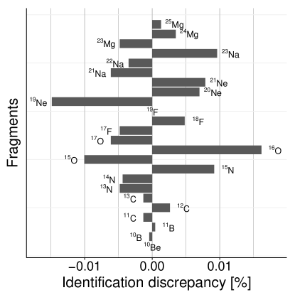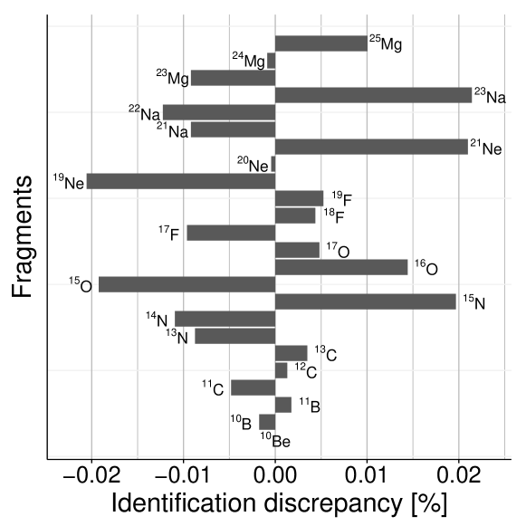In the right panel of fig. 2 we present the identification discrepancy for each fragment due to a noise application. We calculate it as a difference between the originally simulated number of fragments of given A and Z and number of these fragments after noise application and re-classification, normalized to the total number of simulated fragments. Negative values indicate number of fragments that have been underestimated, whereas positive indicate that they have been overestimated. The fragments with A and Z reassigned to simulated data after noise superimposition, will be, from now on, called the reference data. The evolutionary algorithm has been run on an average class laptop. It needed around 10 minutes and 68 iterations to complete the calculations. The initial values of parameters g, $\mu$ and $\lambda$ have all been set to 0.1. Since the aCMA-ES works better when the parameters are the same order of magnitude, parameter $\lambda$ has been scaled by 100. As a result of the algorithm, they have been estimated to 0.252, 0.699 and 0.842, respectively. 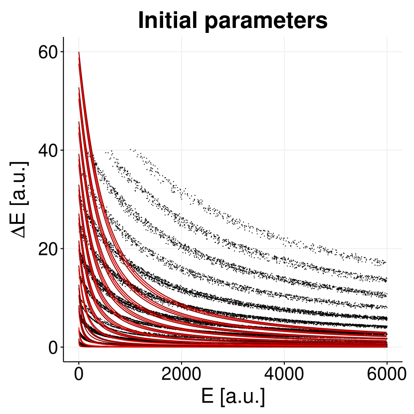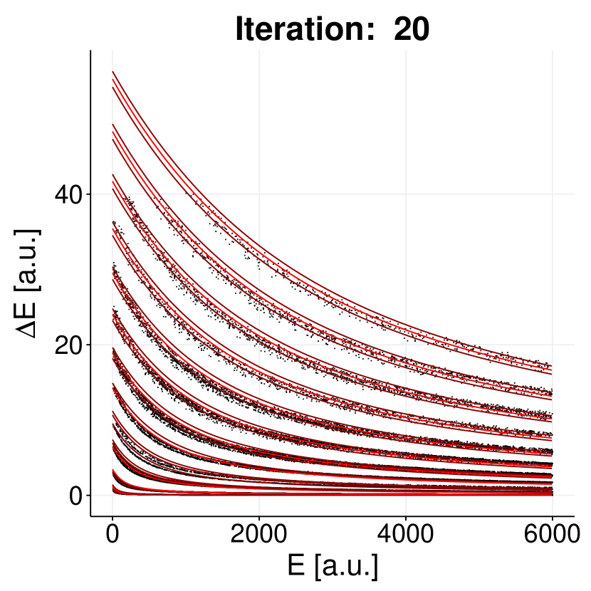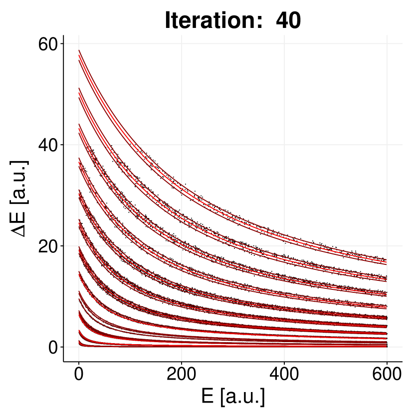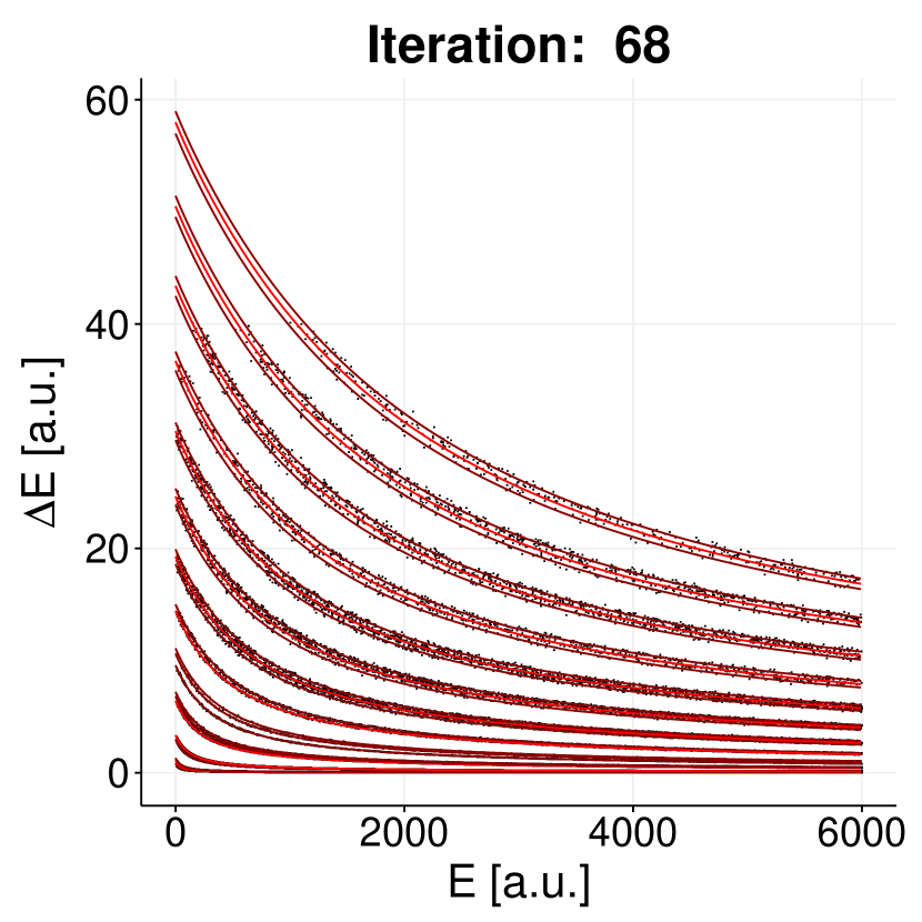In section 4 we show the evolution of those parameters as a function of iteration number. The model function calculated with the initial parameters (a), after the 20th (b), 40th (c) and 68th (d) iteration, plotted on the top of simulated data is shown in fig. 3. It can be seen, that the model function with initial parameters certainly does not describe the simulated data, however after the 20th iteration it decently fits the data. The last two thirds of the iterations are used to fine-tune the parameters. l0.36 Model function parameters evolution: (a) parameter g, (b) parameter $\mu$, (c) parameter $\lambda$ Parameters obtained as the result of the evolutionary algorithm have been used to produce a final mass and charge classification. Fragments with A and Z assigned to simulated data after algorithm performance will be called operational data. We again calculated the identification discrepancy for each fragment, This time it has been calculated as a difference between the simulated data and the operational data. In fig. 4 we present these discrepancies. The function parameters have been reconstructed with high accuracy, it is not surprising therefore, that the data classification efficiency is as high as 99.76$\%$. Fragment charge has been properly assigned to all fragments. 550 fragments, out of 228698, were misidentified in mass, all of them being a species with Z ¿ 4. Compared to the number of fragments misidentified due to noise superposition, this number rose about 49 and that is a 0.214‰ of total number of studied fragments.

(a)

(b)

(c)

(d)

Figure 3: The model function (red lines) calculated with the initial parameters (a), after the 20th (b), 40th (c) and 68th (d) iteration, plotted on the top of simulated data (black points).

Figure 4: Identification discrepancies of particular fragments after final identification process.. Negative values inform that numbers of fragments have been underestimated, positive - that they have been overestimated.

Figure 5: Algorithm performance on simulated data with missing isotopes. Left: missing H and He isotopes. Right: missing Ne, Na and Mg isotopes.

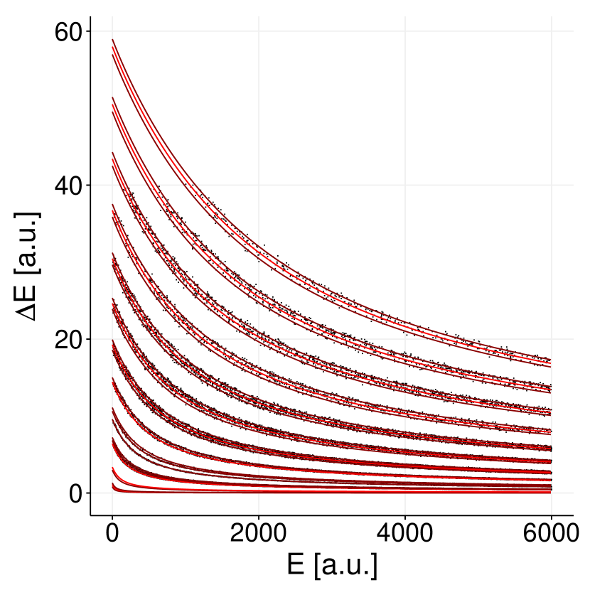
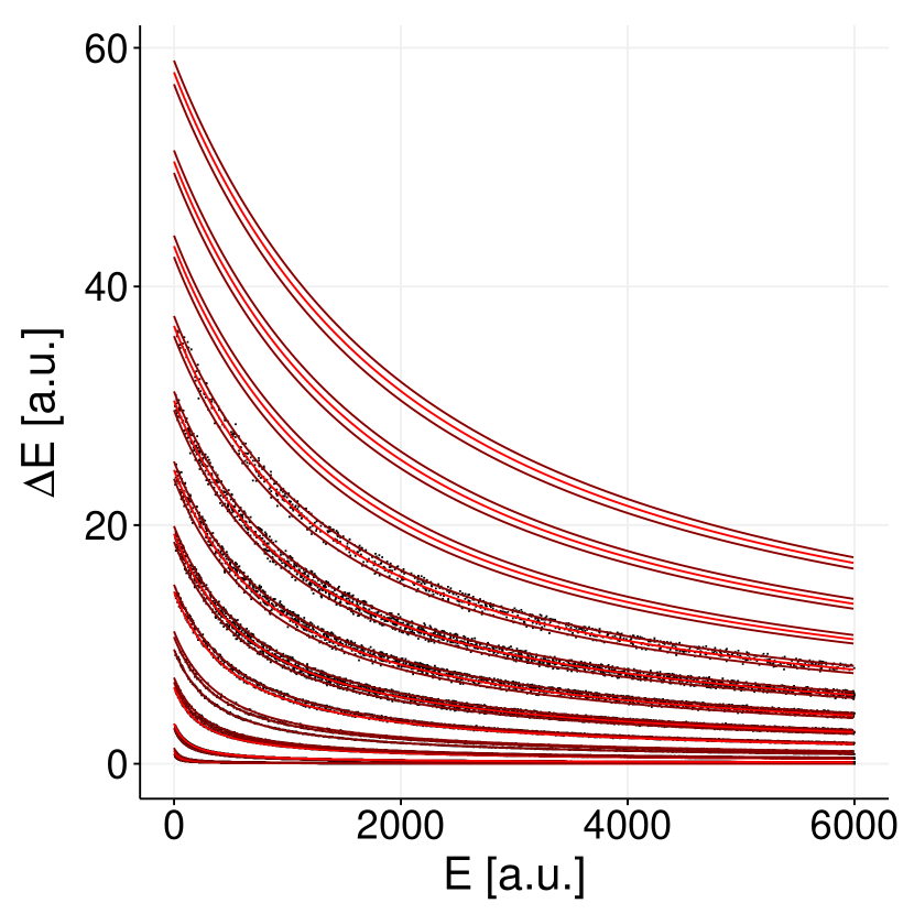
The last test performed was to execute the algorithm on simulated data without some of the isotopes with the model having number of isotope types not changed (${}^{1}_{1}$H up to ${}^{25}_{12}$Mg). In the left hand side of fig. 5 the result of algorithm performance without isotopes of H and He is shown, in the right hand side of fig. 5 the result for simulated data without Ne, Na and Mg isotopes. It can be seen that the algorithm works very well for a such set of data. The conclusion from that test is that in order to identify fragments produced in a given experimental reaction it is necessary to create a model encompassing all isotopes expected in the reaction. Although every telescope detects different number of isotope types, the algorithm should fit the data properly.

5 Summary

The goal of this paper was to present the proof of concept of using an evolutionary strategy in $\Delta$E - E identification procedure. We have simulated labeled data using a model describing $\Delta$E - E correlations. This was followed by applying our algorithm to that data. In this way we have reconstructed the original (simulated) mass (A) and charge (Z) and calculated the efficiency of that reconstruction. None of cited articles in section  1 adressed efficiency, since the authors have applied their methods directly on experimental, not simulated data.

The method presented in this article shows that the agreement between the simulated and operational data is 100$\%$ for charge identification. As presented in section 4, the efficiency of mass identification is 100$\%$ for fragments up to ¹⁰Be. With increasing charge, the distinction between isotopes decreases, which led to lower mass classification efficiency. However, only 0.24$\%$ of isotopes were misidentified in mass, which is a significant result. It is important to emphasize, that in this paper we have tested the model describing linear detectors. In the future work we would like to test the method with various models, including the extended model of $\Delta$E - E relation, (eq. 2) for linear detectors and model with one nonlinear detector (eq.  2 with eq.  3 as a correction). We also would like to test the method sensitivity to various statistics. Finally, we plan to apply the method on experimental data collected by several experiments with various detection arrays.

We would like to thank dr J. B. Natowitz and dr K. Hagel from Cyclotron Institute, Texas A$\&$M University for improving the quality of this paper by sharing their expertise knowledge. Furthermore, we would like to thank groups from University of Silesia and Jagiellonian University involved in the experiments on heavy ion reactions at intermediate energies for their kindness and support of this study.

References

- [1] DW Stracener, DG Sarantites, LG Sobotka, J Elson, JT Hood, Z Majka, V Abenante, A Chbihi, and DC Hensley. Dwarf ball and dwarf wall: Design, instrumentation, and response characteristics of a 4 csi (tl) plastic phoswich multidetector system for light charged particle and intermediate mass fragment spectrometry. Nuclear Instruments and Methods in Physics Research Section A: Accelerators, Spectrometers, Detectors and Associated Equipment, 294(3):485–503, 1990.
- [2] JOEL Pouthas, B Borderie, R Dayras, E Plagnol, MF Rivet, F Saint-Laurent, JC Steckmeyer, G Auger, Ch O Bacri, S Barbey, et al. Indra, a 4 charged product detection array at ganil. Nuclear Instruments and Methods in Physics Research Section A: Accelerators, Spectrometers, Detectors and Associated Equipment, 357(2-3):418–442, 1995.
- [3] K Kwiatkowski, DS Bracken, KB Morley, J Brzychczyk, E Renshaw Foxford, K Komisarcik, VE Viola, NR Yoder, J Dorsett, J Poehlman, et al. The indiana silicon sphere 4 charged-particle detector array. Nuclear Instruments and Methods in Physics Research Section A: Accelerators, Spectrometers, Detectors and Associated Equipment, 360(3):571–583, 1995.
- [4] DG Sarantites, P-F Hua, M Devlin, LG Sobotka, J Elson, JT Hood, DR LaFosse, JE Sarantites, and MR Maier. “the microball” design, instrumentation and response characteristics of a 4-multidetector exit channel-selection device for spectroscopic and reaction mechanism studies with gammasphere. Nuclear Instruments and Methods in Physics Research Section A: Accelerators, Spectrometers, Detectors and Associated Equipment, 381(2-3):418–432, 1996.
- [5] A Pagano, M Alderighi, F Amorini, A Anzalone, L Arena, L Auditore, V Baran, M Bartolucci, I Berceanu, J Blicharska, et al. Fragmentation studies with the chimera detector at lns in catania: recent progress. Nuclear Physics A, 734:504–511, 2004.
- [6] S Wuenschel, K Hagel, R Wada, JB Natowitz, SJ Yennello, Z Kohley, C Bottosso, LW May, WB Smith, DV Shetty, et al. Nimrod–isis, a versatile tool for studying the isotopic degree of freedom in heavy ion collisions. Nuclear Instruments and Methods in Physics Research Section A: Accelerators, Spectrometers, Detectors and Associated Equipment, 604(3):578–583, 2009.
- [7] R Bougault, G Poggi, S Barlini, B Borderie, G Casini, A Chbihi, N Le Neindre, M Pârlog, G Pasquali, S Piantelli, et al. The fazia project in europe: R&d phase. 2014.
- [8] J Łukasik, P Pawłowski, A Budzanowski, B Czech, I Skwirczyńska, Janusz Brzychczyk, Marek Adamczyk, Sebastian Kupny, Paweł Lasko, Zbigniew Sosin, et al. Kratta, a versatile triple telescope array for charged reaction products. Nuclear Instruments and Methods in Physics Research Section A: Accelerators, Spectrometers, Detectors and Associated Equipment, 709:120–128, 2013.
- [9] GW Butler, AM Poskanzer, DA Landis, and J Galin. X. tarrago for example. Nucl. Instr. and Meth, 89:189, 1970.
- [10] L Tassan-Got. A new functional for charge and mass identification in e–e telescopes. Nuclear Instruments and Methods in Physics Research Section B: Beam Interactions with Materials and Atoms, 194(4):503–512, 2002.
- [11] N Le Neindre, M Alderighi, A Anzalone, R Barnà, M Bartolucci, I Berceanu, B Borderie, R Bougault, M Bruno, G Cardella, et al. Mass and charge identification of fragments detected with the chimera silicon–csi (tl) telescopes. Nuclear Instruments and Methods in Physics Research Section A: Accelerators, Spectrometers, Detectors and Associated Equipment, 490(1):251–262, 2002.
- [12] PF Mastinu, PM Milazzo, M Bruno, and M D’agostino. A procedure to calibrate a multi-modular telescope. Nuclear Instruments and Methods in Physics Research Section A: Accelerators, Spectrometers, Detectors and Associated Equipment, 371(3):510–513, 1996.
- [13] J Dudouet, D Juliani, M Labalme, JC Angélique, B Braunn, J Colin, D Cussol, Ch Finck, JM Fontbonne, H Guérin, et al. Comparison of two analysis methods for nuclear reaction measurements of 12 c+ 12 c interactions at 95mev/u for hadron therapy. Nuclear Instruments and Methods in Physics Research Section A: Accelerators, Spectrometers, Detectors and Associated Equipment, 715:98–104, 2013.
- [14] T Cap, K Siwek-Wilczyńska, I Skwira-Chalot, J Wilczyński, CHIMERA Collaboration, et al. Detection and identification of large fragments from the partitioning of the 197au+ 197au system at 23a mev. Physica Scripta, 2013(T154):014007, 2013.
- [15] D Gruyer, E Bonnet, A Chbihi, JD Frankland, S Barlini, B Borderie, R Bougault, JA Duenas, Emmanuelle Galichet, A Kordyasz, et al. New semi-automatic method for reaction product charge and mass identification in heavy-ion collisions at fermi energies. Nuclear Instruments and Methods in Physics Research Section A: Accelerators, Spectrometers, Detectors and Associated Equipment, 2016.
- [16] Oskar Wyszyński. Evolutionary algorithm for particle trajectory reconstruction within inhomogeneous magnetic field in the na61/shine experiment at cern sps. Schedae Informaticae, 2015(Volume 24):159–177, 2016.
- [17] T Shimoda, M Ishihara, K Nagatani, and T Nomura. Simple e- e particle identification with a wide dynamic range. Nuclear Instruments and Methods, 165(2):261–264, 1979.
- [18] JB Birks and FWK Firk. The theory and practice of scintillation counting. Physics Today, 18:60, 1965.
- [19] N. Hansen. The CMA evolution strategy: a comparing review. In J.A. Lozano, P. Larranaga, I. Inza, and E. Bengoetxea, editors, Towards a new evolutionary computation. Advances on estimation of distribution algorithms, pages 75–102. Springer, 2006.
- [20] N. Hansen and A. Ostermeier. Adapting arbitrary normal mutation distributions in evolution strategies: The covariance matrix adaptation. In Proceedings of the 1996 IEEE International Conference on Evolutionary Computation, pages 312–317. IEEE, 1996.
- [21] N. Hansen and A. Ostermeier. Completely derandomized self-adaptation in evolution strategies. Evolutionary Computation, 9(2):159–195, 2001.
- [22] C. Igel, N. Hansen, and S. Roth. Covariance matrix adaptation for multi-objective optimization. Evolutionary Computation, 15(1):1–28, 2007.
- [23] R Core Team. R language definition. Vienna, Austria: R foundation for statistical computing, 2000.
- [24] Emmanuel Benazera. libcmaes: Multithreaded c++ 11 implementation of cma-es family for optimization of nonlinear non-convex blackbox functions, 2014.
- [25] Dirk Eddelbuettel, Romain François, J Allaire, John Chambers, Douglas Bates, and Kevin Ushey. Rcpp: Seamless r and c++ integration. Journal of Statistical Software, 40(8):1–18, 2011.
- [26] Grahame A. Jastrebski and Dirk V. Arnold. Improving evolution strategies through active covariance matrix adaptation. In Evolutionary Computation, 2006. CEC 2006. IEEE Congress on, pages 2814–2821. IEEE, 2006.
- [27] Nikolaus Hansen and Raymond Ros. Benchmarking a weighted negative covariance matrix update on the bbob-2010 noiseless testbed. In Proceedings of the 12th annual conference companion on Genetic and evolutionary computation, pages 1673–1680. ACM, 2010.