Far-infrared metallicity diagnostics: Application to local ultraluminous infrared galaxies

Abstract

The abundance of metals in galaxies is a key parameter which permits to distinguish between different galaxy formation and evolution models. Most of the metallicity determinations are based on optical line ratios. However, the optical spectral range is subject to dust extinction and, for high-$z$ objects ($z>3$), some of the lines used in optical metallicity diagnostics are shifted to wavelengths not accessible to ground based observatories. For this reason, we explore metallicity diagnostics using far-infrared (IR) line ratios which can provide a suitable alternative in such situations. To investigate these far-IR line ratios, we modeled the emission of a starburst with the photoionization code cloudy. The most sensitive far-IR ratios to measure metallicities are the [O iii]52 $\mu$m and 88 $\mu$m to [N iii]57 $\mu$m ratios. We show that this ratio produces robust metallicities in the presence of an AGN and is insensitive to changes in the age of the ionizing stellar. Another metallicity sensitive ratio is the [O iii]88 $\mu$m/[N ii]122 $\mu$m ratio, although it depends on the ionization parameter. We propose various mid- and far-IR line ratios to break this dependency. Finally, we apply these far-IR diagnostics to a sample of 19 local ultraluminous IR galaxies (ULIRGs) observed with Herschel and Spitzer. We find that the gas-phase metallicity in these local ULIRGs is in the range $0.7<Z_{\rm gas}/$$Z_{\rm\odot}$$<1.5$, which corresponds to $8.5<12+\log({\rm O/H})<8.9$. The inferred metallicities agree well with previous estimates for local ULIRGs and this confirms that they lie below the local mass-metallicity relation.

1 Introduction

The abundance of metals in a galaxy is an evidence of its past history. This is because observed gas metallicities are the direct result of the metal enrichment due to the stellar nucleosynthesis and posterior dispersion of these metals in the interstellar medium (ISM) through stellar winds, supernovae, and planetary nebulae, the inflow of intergalactic metal poor gas, the outflow of metal rich material, and the minor/major merger history. Therefore, the determination of metallicities puts constraints on the star-formation (SF) and intergalactic accretion histories of galaxies, and consequently, these determinations are fundamental for models of formation and evolution of galaxies (e.g., Brooks et al. 2007; Finlator & Davé 2008; Lilly et al. 2013).

Methods to derive gas-phase metallicities using ultraviolet (UV) and optical transitions have been widely used in the last several decades (e.g., Pagel et al. 1979; Alloin et al. 1979; Edmunds & Pagel 1984; Skillman 1989). However, an intrinsic limitation of these methods is that UV and optical transitions are susceptible to dust extinction. This is important, since a large part of the SF in the Universe occurs in dust obscured environments and also because, at $z\sim 1-2$, close to the peak of the cosmic SF history, the dust attenuation reaches its maximum value (e.g., Madau & Dickinson 2014; Casey et al. 2014). In these cases, UV and optical methods to derive metallicities might be uncertain.

To minimize the effect of the extinction in metallicity determinations, it is possible to use far-infrared (far-IR) atomic fine-structure transitions which are much less susceptible to extinction than UV and optical transitions (e.g., Liu et al. 2001, Nagao et al. 2011, 2012; Béthermin et al. 2016). For local galaxies, these far-IR transitions are only accessible to space observatories like the Infrared Space Observatory (ISO; Kessler et al. 1996), Spitzer (Werner et al. 2004), AKARI (Murakami et al. 2007), or Herschel (Pilbratt et al. 2010). For high-$z$ objects, the far-IR spectral range shifts into the observed sub-millimeter and it is possible to observe it with the Atacama Large Millimeter Array (ALMA) or with the Northern Extended Millimeter Array (NOEMA) for instance. As a result, it is likely that many measurements of far-IR transitions will become available for high-$z$ objects in the near future. Also, due to the atmospheric sub-mm absorption bands, only certain combinations of far-IR transitions can be observed with ALMA as a function of redshift, hence it is necessary to identify which diagnostics are the best ones to optimize future observations.

In this paper, we compute cloudy (Ferland et al. 2013) models of H ii regions and AGN to investigate which far-IR line ratios can be used as metallicity diagnostics. We consider a wide range of gas volume densities and ionization parameters as well as explore the effect of varying the age of the ionizing stellar population and the slope of the AGN ionizing continuum. We then apply the obtained far-IR metallicity diagnostics to a sample of local ultraluminous IR galaxies (ULIRGs; $L_{\rm IR}>10^{12}$ $L_{\rm\odot}$) observed with Herschel.

This paper is organized as follows: The photoionization models are described in Section 2. We discuss the far-IR gas density, ionization parameter, and metallicity ratio diagnostics as well as the impact of an AGN in the far-IR line ratios in Section 3. We apply these models to a sample of local ULIRGs in Section 4. In Section 5, we summarize the main results of this work.

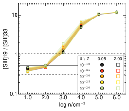
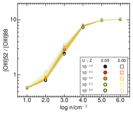
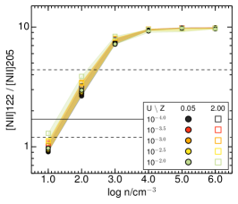
Figure 1: [S iii]19 $\mu$m/[S iii]33 $\mu$m, [O iii]52 $\mu$m/[O iii]88 $\mu$m, and [N ii]122 $\mu$m/[N ii]205 $\mu$m ratios (from left to right) as a function of the input atomic hydrogen density of the models. For each density, we group the models with the same ionization parameter but different gas metallicity and plot the ratios for the lowest and highest metallicities with a filled circle and an empty square, respectively. The color coding (black, red, orange, yellow, and green) indicates the ionization parameter ($\log U=$ –4.0, –3.5, –3.0, –2.5, and –2.0, respectively). The colored shaded areas mark the range of ratios predicted by the models with the same ionization parameter but different metallicities. The horizontal solid and dashed lines indicate the median and range of observed ratios, respectively, in our sample of local ULIRGs (see Section 4).

2 Far-IR line emission modeling

We use the spectral synthesis code cloudy version 13.04 (Ferland et al. 2013) to model the far-IR fine-structure emission lines produced in H ii regions and in the presence of an AGN as a function of the metallicity, density, and ionization parameter. Similar models for H ii regions were presented by Nagao et al. (2011). In general, we follow their work, although we only use transitions entirely produced in the ionized gas. Therefore, we stop our models when the H⁺ abundance drops below 1% and do not attempt to model the photo-dissociation region (PDR) emission. This is done to simplify the modeling and to avoid assumptions on the relation between the PDR and ionized gas physical conditions.

2.1 Starburst photoionization models

We assume a constant pressure slab model illuminated by the spectrum of a continuous burst of SF. This illuminating spectrum was calculated using starburst99 version 7 (Leitherer et al. 1999) assuming continuous SF with a Kroupa (2001) initial mass function with an upper stellar mass boundary of 100 $M_{\rm\odot}$. This is an average spectrum representing the integrated emission of a galaxy with stellar populations of different ages. We also explore the dependence on the stellar age by simulating an instantaneous burst of SF with starburst99 with ages between 1 and 12 Myr. We produce the spectra for the five stellar metallicities ($Z_{\rm star}$ = 0.05$Z_{\rm\odot}$, 0.2$Z_{\rm\odot}$, 0.4$Z_{\rm\odot}$, $Z_{\rm\odot}$, and 2$Z_{\rm\odot}$) available for the Geneva evolutionary tracks (Meynet et al. 1994).

We matched the gas-phase abundance, $Z_{\rm gas}$, to that of the incident stellar spectrum. For the solar metallicity, we used the Asplund et al. (2009) values ($12+\log({\rm O/H})_{\odot}=8.69\pm 0.05$). For the remaining metallicities, we assume that the abundances scale as $Z_{\rm gas}$/$Z_{\rm\odot}$ for all the elements except for He and N. For He, we use the relation given by Dopita et al. (2006):

$${\rm He}/{\rm H}=0.0737+0.024\,Z_{\rm gas}/\hbox{$Z_{\rm\odot}$}$$ (1)

which takes into account the primordial He abundance and the He primary nucleosynthesis. For N, we use the Pilyugin et al. (2014) fit to the observed relation between N/H and O/H in nearby galaxies:

$$\log\frac{{\rm N}}{\rm H}=-3.96+2.47\,\log\frac{Z_{\rm gas}}{\hbox{$Z_{\rm\odot}$}} ~{}~{}{\rm for}~{}Z_{\rm gas}\geq 0.25\hbox{$Z_{\rm\odot}$}$$ (2)

$$\log\frac{{\rm N}}{\rm H}=-4.85+\log\frac{Z_{\rm gas}}{\hbox{$Z_{\rm\odot}$}} ~{}~{}{\rm for}~{}Z_{\rm gas}<0.25\hbox{$Z_{\rm\odot}$}.$$

Two equations are needed to model the N abundance because at high-metallicities ($Z>0.25\hbox{$Z_{\rm\odot}$}$), the contribution from secondary N becomes important making the N abundance to increase faster than the O one.

The stellar metallicities of the starburst99 models assume that the mass fraction of metals with respect to hydrogen, $Z$, is 0.020, which is slightly higher than the value we use for the gas phase metallicities ($Z=0.018$; Asplund et al. 2009). This implies that the stellar spectrum will be slightly softer than it should be for a given metallicity, although this does not affect the model results (Dopita et al. 2006).

The models include dust grains with a gas-to-dust mass ratio (G/D) adjusted following the value observed in local galaxies as a function the metallicity. In particular, we use the broken power-law fit using $X_{\rm CO,Z}$ presented by Rémy-Ruyer et al. 2014:

$$\log{\rm G}/{\rm D}=2.21-\log\frac{Z_{\rm gas}}{\hbox{$Z_{\rm\odot}$}} ~{}~{}{\rm for}~{}Z_{\rm gas}\geq 0.25\hbox{$Z_{\rm\odot}$}$$ (3)

$$\log{\rm G}/{\rm D}=0.96-3.10\,\log\frac{Z_{\rm gas}}{\hbox{$Z_{\rm\odot}$}} ~{}~{}{\rm for}~{}Z_{\rm gas}<0.25\hbox{$Z_{\rm\odot}$}.$$

Depletion of metals onto dust grains is included using the standard depletion factors listed in the cloudy documentation (Hazy1) except for O and N. For these two elements, we assume no depletion in order to match the gas-phase abundances in the models with those observed (Pilyugin et al. 2014).

We created a grid of models varying three input parameters: the metallicity $Z_{\rm gas}$, the gas volume density $n_{\rm H}$, and the ionization parameter $U$. The ionization parameter is a dimensionless parameter defined as $U=\Phi/(c\,n_{\rm H})$, where $\Phi$ is the flux of ionizing photons in cm^-2 s^-1 and $c$ the speed of light. The value of $U$ determines the intensity of the incident spectrum.

We explore a wide range of ionization parameters from $\log U=-4$ to $-2$ in steps of 0.5 dex and gas volume densities from $\log n_{\rm H}/{\rm cm^{-3}}=1$ to 6 (this density value corresponds to density at the illuminated face of the slab in our constant pressure models) in steps of 1 dex. For the metallicities, we used $Z_{\rm gas}$ = 0.05$Z_{\rm\odot}$, 0.2$Z_{\rm\odot}$, 0.4$Z_{\rm\odot}$, $Z_{\rm\odot}$, and 2$Z_{\rm\odot}$, similar to the metallicities of stellar spectra. The predicted mid- and far-IR line ratios for the grid of models are listed in Appendix A.

2.2 AGN photoionization models

We produced AGN photoionization models following the prescription given in Section 2.1, but replacing the illuminating spectrum by a broken power-law with an index $\alpha_{\rm AGN}=-1.4$ ($f_{\nu}\propto\nu^{\alpha}$) between 10 $\mu$m and 50 keV, $\alpha=2.5$ for $\lambda>$10 $\mu$m, and $\alpha=-2.0$ for $E>50$ keV. We also ran models with $\alpha_{\rm AGN}$ between –2.5 and –0.5 (e.g., Moloney & Shull 2014) to investigate the effect of varying the AGN radiation field hardness. The range of the ionization parameters, $\log\,U=$–3.0 to –1.6, is that of typical AGN (e.g., Meléndez et al. 2014). The remaining input parameters of the model (gas-phase abundances, stopping criteria, gas density range, dust grains, etc.) are the same that we used for the starburst models. In Appendix B, we plot line ratios presented in the main text for the starburst models and list the numerical values of the ratios predicted by these AGN models.

3 Results

In this section, we present the main results of the photoionization models described in Section 2. We use as reference the continuous SF model and, in Sections 3.4 and 3.5, we discuss the effect of varying the age of the ionizing stellar population and in the presence of an AGN. First, we discuss line ratios that can be used to derive the gas density and ionization parameter. Then, we present ratios that can be used to constrain gas metallicities.

3.1 Gas density determination

The ratio of mid- and far-IR fine-structure transitions from the same ion (e.g., [S iii], [O iii], [N ii]) but with different critical densities allows the determination of the emitting gas density (e.g., Draine 2011). In Figure 1, we plot three of these mid- and far-IR diagnostics. Although our models are not constant density models, these ratios are almost determined by the gas density at the illuminated face of the modeled slab. For a given density, the scatter of these ratios due to variations of the ionization parameter and gas metallicity is only 10–20%.

3.2 Ionization parameter determination

Besides the gas density, the other key parameter that defines the photoinization model is the ionization parameter $U$. We explored all the possible combinations between mid- and far-IR transitions looking for ratios that correlate with the ionization parameter. The ratio that is best correlated with $U$ is the [S iv]11 $\mu$m/[Ne iii]16 $\mu$m ratio (see Figure 2). This ratio is almost independent of the gas density for the considered reduced range ($1<\log n_{\rm H}{\rm(cm^{-3})}<4$; see Section 4), but it shows a mild dependence on the metallicity for $\log U$ values higher than –3.0.

Another ratio that is sometimes used to measure the ionization parameter is the [Ne ii]13 $\mu$m/[Ne iii]16 $\mu$m ratio (e.g., Snijders et al. 2007; Nagao et al. 2011; Meléndez et al. 2014). However, this ratio has a much stronger dependence on the metallicity (Figure 3). This is because the fraction of photons that are able to ionize Ne⁺, and therefore lead to [Ne iii] emission, is notably higher for low metallicity starbursts. That is, the [Ne ii]13 $\mu$m/[Ne iii]16 $\mu$m ratio is very sensitive to the hardness of the ionizing radiation (e.g., Rigby & Rieke 2004). Because of the strong dependence on $Z_{\rm gas}$ of this ratio when $Z_{\rm gas}>$0.4$Z_{\rm\odot}$, it is not useful to estimate $U$ in the high metallicity range. However, it can provide relatively accurate estimates of $U$ for $Z_{\rm gas}<$0.4$Z_{\rm\odot}$ because the ratio between the number of photons able to ionize Ne⁰ and Ne⁺ remains approximately constant for those metallicities.

None of the far-IR line ratios are suitable to constrain the ionization parameter independently of the metallicity (see also Nagao et al. 2011). However, if a rough estimate of the metallicity is available, then it is possible to use the [N ii]122 $\mu$m/[N iii]57 $\mu$m and [O iii]88 $\mu$m/[N ii]122 $\mu$m ratios to constrain the ionization parameter (Figure 4).

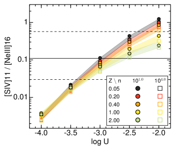
Figure 2: [S iv]11 $\mu$m/[Ne iii]16 $\mu$m ratio as a function of the ionization parameter $U$. The symbols are as in Figure 1, but here we group the models by their metallicity and the shaded area is given by the density dependence and the horizontal solid line is the mean ratio estimated using the Kaplan-Meier estimator. The color coding (black, red, orange, yellow, and green) indicates the gas metallicities ($Z/Z_{\odot}=$ 0.05, 0.2, 0.4, 1, 2, respectively).

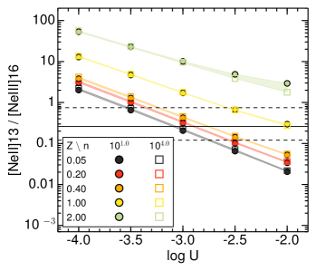
Figure 3: [Ne ii]13 $\mu$m/[Ne iii]16 $\mu$m ratio as a function of the ionization parameter $U$. The symbols are as in Figure 2.

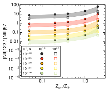
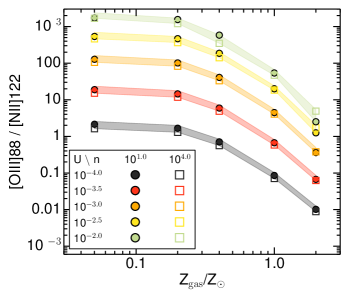
Figure 4: [N ii]122 $\mu$m/[N iii]57 $\mu$m (top panel) and [O iii]88 $\mu$m/[N ii]122 $\mu$m (bottom panel) ratios as a function of the metallicities. The symbols are as in Figure 2, but here we group the models by their ionization parameter and the shaded area is given by the density dependence. The color coding (black, red, orange, yellow, and green) indicates the ionization parameter ($\log U=$ –4.0, –3.5, –3.0, –2.5, and –2.0, respectively)

3.3 Metallicity determination

3.3.1 [O iii] to [N iii] ratios

We used the predictions of the models described in Section 2 to identify far-IR transitions which can be used to measure the gas metallicity. We find that the best ratios are those involving the [O iii]52 $\mu$m and 88 $\mu$m and [N iii]57 $\mu$m transitions.

These line ratios trace the abundance ratio between O⁺⁺ and N⁺⁺, which is a good proxy of the total O to N abundance ratio in H ii regions. O and N have similar ionization potentials for their neutral (13.6 and 14.5 eV, respectively), single (35 and 30 eV), and double (55 and 47 eV) ionized stages, which are the dominant stages found in H ii regions for these two elements. For this reason, both have similar ionization structures, independent of the hardness of the radiation field and the ionization parameter, and, therefore, the O⁺⁺ to N⁺⁺ ratio can be used to measure the global O to N ratio.

In our models, the O abundance is proportional to $Z_{\rm gas}$ whereas the N abundance increases faster than $Z_{\rm gas}$ due to the secondary N production when $Z_{\rm gas}\geq 0.25$$Z_{\rm\odot}$ (see Section 2 and Equation 3). Therefore, the O/N abundance ratio varies with $Z_{\rm gas}$ and can be used to indirectly determine the gas metallicity for $Z_{\rm gas}\gtrsim 0.25$$Z_{\rm\odot}$.

The [O iii] to [N iii] ratios have been already identified as far-IR metallicity tracers (e.g., Liu et al. 2001; Nagao et al. 2011), although they are strongly dependent on the electron density (see left and middle panels of Figure LABEL:fig:o3_n3). However, for a fixed metallicity, the density dependence of the [O iii]52 $\mu$m/[N iii]57 $\mu$m ratio is opposite of that of the [O iii]88 $\mu$m/[N iii]57 $\mu$m ratio because the [O iii]52 $\mu$m (88 $\mu$m) is enhanced at high (low) densities (see Figures 1 and LABEL:fig:o3_n3). This is because of the higher critical density of the [O iii]52 $\mu$m transition ($\sim$4000 cm^-3; e.g., Fernández-Ontiveros et al. 2016) compared to that of the [O iii]88 $\mu$m transition ($\sim$500 cm^-3). Based on this fact, previous works used the ([O iii]52 $\mu$m$+$[O iii]88 $\mu$m)/[N iii]57 $\mu$m flux ratio to break the density degeneracy, but some scatter is still present (see figure 5 of Nagao et al. 2011). To further improve this metallicity calibrator, we identify the linear combination of the [O iii] fluxes in the ($a\times$[O iii]88 $\mu$m$+$[O iii]52 $\mu$m)/[N iii]57 $\mu$m ratio that minimizes the scatter of the predicted ratio for a given gas metallicity. In this calculation, we only consider models with $n_{\rm H}\leq 10^{4}$ cm^-3 as expected in H ii regions. The best result is obtained with the ($2.2\times$[O iii]88 $\mu$m$+$ [O iii]52 $\mu$m)/[N iii]57 $\mu$m ratio (right panel of Figure LABEL:fig:o3_n3). This linear combination reduces the scatter of the correlation to 0.2 dex for a given ratio with respect the 0.4 dex scatter using the direct addition of the [O iii] fluxes.

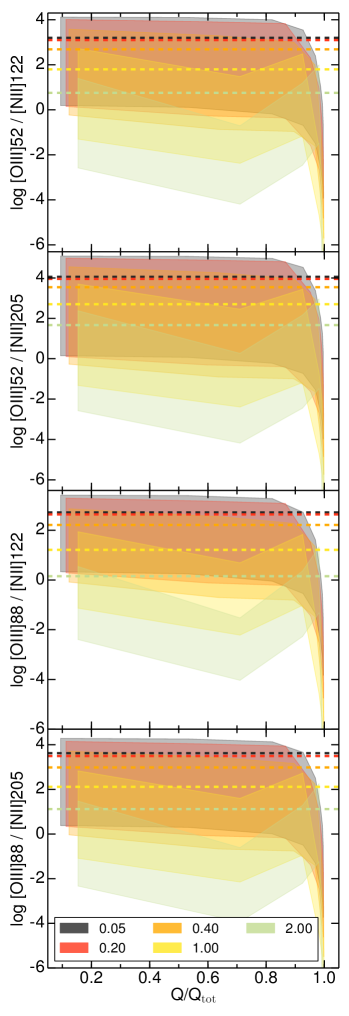
Figure 5: [O iii] to [N ii] ratios. Symbols are as in Figure LABEL:fig:o3_n3_q0.

3.3.2 [O iii] to [N ii] ratios

The far-IR [N iii]57 $\mu$m and [O iii]52 $\mu$m transitions are difficult to observe from the ground. Only for $z$>5.2 sources, these transitions are shifted into the ALMA band 10 observing range. For this reason, we also investigate alternative ratios involving transitions more easily accessible to ground sub-mm observatories also for lower-$z$ galaxies.

Analyzing all the possible combinations of line ratios predicted by our models, the best candidates are ratios between the far-IR [O iii] and [N ii] transitions. In Figures 4 and LABEL:fig:Z_o3, we plot the [O iii] to [N ii] ratios. In contrast to the [O iii]/[N iii]57 $\mu$m ratios discussed in the previous section, the [O iii]/[N ii] ratios have a strong dependence on the ionization parameter. This is because the relative amount of O⁺⁺ and N⁺ depends on $U$ (see also Section 3.3.1). All these ratios also depend on the gas density because of the different critical densities of the transitions (e.g., Fernández-Ontiveros et al. 2016). The ratio less dependent on the gas density is the [O iii]88 $\mu$m/[N ii]122 $\mu$m ratio since both transitions have critical densities around 300–500 cm^-3. The other two transitions have higher ([O iii]52 $\mu$m, $\sim$4000 cm^-3) and lower ([N ii]205 $\mu$m, $\sim$50 cm^-3) critical densities, respectively.

Therefore, if a value for the ionization parameter is assumed (based on the observations of other transitions, e.g., Section 3.2), it is possible to derive the gas metallicity using these ratios. In particular, the [O iii]88 $\mu$m/[N ii]122 $\mu$m ratio would be the best option since it is the less dependent on the gas density.

3.4 Stellar Age

In the previous section, we have assumed that the ionizing radiation seen by the gas clouds is that produced by continuous SF. This is reasonable when the integrated emission of galaxies is analyzed. However, when the far-IR emission from individual H ii regions is studied, the age of the ionizing stellar population might affect the observed line ratios. For this reason, we investigate the variation of the metallicity ratio diagnostics described before (i.e., [O iii] to [N iii] and [O iii] to [N ii] ratios) for an instantaneous burst of SF as a function of the age of the ionizing population.

In Figure LABEL:fig:o3_n3, we present the evolution of the [O iii] to [N iii] ratios as a function of the burst age. The global trend observed in these ratios for the continuous SF models, that is, higher ratios at lower metallicities, is also visible in this figure. However, these ratios have a strong dependence on the stellar population age. Also, a degeneracy between age and metallicity is observed: a low-metallicity region produces line ratios equivalent to a younger high-metallicity region.

Time evolution of these ratios exists, but in reality, it will be hard to observe. Star-forming regions emit ionizing photons during a brief period and after $\sim$6.5 Myr, they have emitted $>$95% of the total ionizing photons (e.g., Dopita et al. 2006). This means that atomic transitions produced in ionized gas, like those of [O iii] and [N iii], are primarily produced during $\sim$6 Myr. To investigate ratio variations in a more meaningful way, we plot in Figure LABEL:fig:o3_n3_q0 these ratios as a function of the cumulative fraction of ionizing photons emitted by the starburst ($Q/Q_{\rm tot}$). In this plot, the ratios appear almost flat (a factor of 2 variation). That is, when these lines can be measured in star-forming regions, their ratios remain approximately constant, and, therefore, these ratios are not very sensitive to the age of the ionizing stellar population.

Similarly, in Figure 5, we plot the [O iii] to [N ii] ratios as function of $Q/Q_{\rm tot}$. In this case, the variation of the ratios is considerably higher for the $Z\geq\hbox{$Z_{\rm\odot}$}$ models (a factor of 150). At low-metallicities, however, the variation with $Q/Q_{\rm tot}$ is smaller ($<5$) and the main dispersion in the predicted ratios comes from the different values of $U$ and $n$ (see Section 3.3.2). Therefore, once a value of $U$ and $n_{\rm H}$ is estimated (see also Section 3.3.2), a rough value for the metallicity can be derived from these ratios independently of the SF history.

3.5 AGN

So far, we have only considered the ionizing radiation from young stars. However, it is interesting to investigate the effect of an AGN in these ratios. To do so, we use the grid of AGN photoionization models presented in Section 2.2.

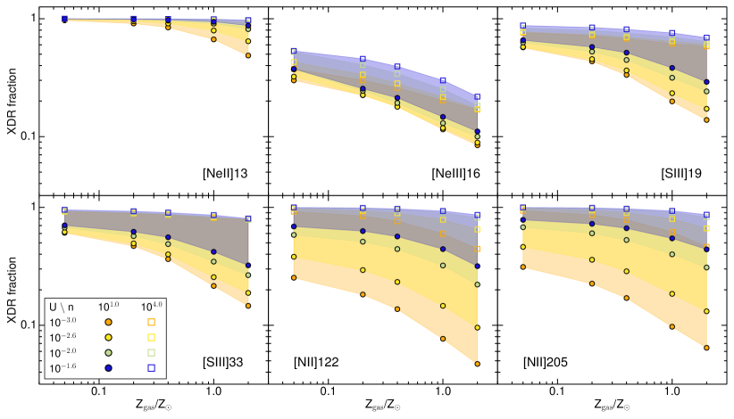
Figure 6: Fraction of the line emission produced in the XDR for the AGN models with $\alpha_{\rm AGN}=-1.4$. Only transitions with significant emission originated in the XDR ([Ne ii]13 $\mu$m, [Ne iii]16 $\mu$m, [S iii]19 $\mu$m, [S iii]33 $\mu$m, [N ii]122 $\mu$m, and [N ii]205 $\mu$m) are included in this figure. The symbols are as in Figure 4.

3.5.1 Emission from X-ray dominated regions

The ionizing spectrum of AGN includes strong X-ray emission. This differs from the spectrum produced in young starbursts which does not have significant X-ray emission. X-ray photons can penetrate deeper in the gas clouds than UV photons because the photoionization cross sections of H and He are greatly reduced at X-ray energies. This implies that X-ray photons can ionize atoms at high column densities and lead to line emission by ionized species in regions where H is mainly atomic neutral. The effects of the X-ray irradiation of the ISM (X-ray dominated regions; XDR) have been widely discussed in the past (e.g, Maloney et al. 1996; Meijerink et al. 2007; Glassgold et al. 2007; Abel et al. 2009; Ádámkovics et al. 2011; Ferland et al. 2013), so we do not discuss them here in detail. However, due to the stopping criterion of our models (H⁺ abundance $<$ 1%), the AGN models include an XDR and some of the IR transitions discussed in this work might be produced there instead of being produced in the ionized gas. Ratios combining transitions from the XDR and the ionized region are subject to larger uncertainties than ionized only ratios because the XDR contribution to these lines should be estimated independently.

To quantify the fraction of the IR line emission produced in XDRs in our models, we first defined the interface between the ionized gas and the XDR as the depth in the cloud where the H ionization goes from being dominated by photoionizations to being dominated by secondary ionizations. This interface exists because, closer to the AGN, H is mainly photoionized by UV photons, but when all the ionizing UV photons have been absorbed, H becomes predominantly ionized by high energy secondary electrons derived from energetic X-ray ionizations. Then, we compute the fraction of line emission produced in the XDR with respect to the total line emission.

Using the $\alpha_{\rm AGN}=-1.4$ models, we find that some transitions ([S iv]11 $\mu$m, [O iii]52 $\mu$m, [N iii]57 $\mu$m, [O iii]88 $\mu$m) are solely produced in the H⁺ region with a negligible contribution from the XDR. For harder AGN radiation fields (higher $\alpha_{\rm AGN}$), some emission from these lines originate in the XDR, but it represents less than 1% of the integrated line emission.

In Figure 6, we plot the XDR fraction for the rest of IR transitions discussed in this work. In general, the XDR contribution for a given transition increases with decreasing metallicities and with increasing gas densities. In both cases, this is because the column density of the atomic phase of the XDR, where these IR transitions originate, increases. This increase is caused by the less efficient gas cooling at low metallicities and high densities (e.g., Draine 2011), which results in higher equilibrium temperatures. And, therefore, the transition from the atomic to the molecular phase, which occurs when $T<500$ K (Cazaux & Tielens 2004), appears deeper in the gas cloud.

Neon transition are known to be enhanced in XDRs (e.g., Glassgold et al. 2007). In our models, the [Ne ii]13 $\mu$m transition mainly arises from the XDR ($>$80%) except for high-metallicity low-density gas where the XDR fraction goes down to $\sim$50%. The XDR contribution to [Ne iii]16 $\mu$m is lower than that of the [Ne ii] transition. It varies between 10–20% for high-metallicity and between 30–60% for the low-metallicity models.

For the two mid-IR [S iii] transitions, the XDR contribution is intermediate between the [Ne ii]13 $\mu$m and [Ne iii]16 $\mu$m cases. Finally, the two far-IR [N ii] transitions have XDR contributions which are highly dependent on the metallicity, density, and ionization parameter. For instance, in the high-metallicity regime, the [N ii] XDR fraction varies from $<$10% to almost 100%. Therefore, in order to use metallicity diagnostics involving far-IR [N ii] transitions in AGNs, the XDR contribution to these lines should be previously estimated.

3.5.2 AGN effects on diagnostic diagrams

For the density diagnostics shown in Figure 1, the AGN models produce similar ratios although the scatter in these relations is increased with values varying up to a factor of 2-4 for the same initial gas density.

Regarding the ionization parameter diagnostics (Figures 2 and 3), the [S iv]11 $\mu$m/[Ne iii]16 $\mu$m ratio saturates for values of $\log\,U>-2$, so it is insensitive to the high ionization parameters that might be present in AGN. But this ratio is also affected by the XDR contribution to the [Ne iii]16 $\mu$m emission (Section 3.5.1) and should be used with caution.

The relation between the [Ne ii]13 $\mu$m/[Ne iii]16 $\mu$m ratio and $U$ is relatively flat and dominated by the scatter due to density and metallicity variations in the AGN models. We note that this behavior differs from the single-zone AGN model presented by Meléndez et al. (2014). In their figure 1, the [Ne ii]13 $\mu$m/[Ne iii]16 $\mu$m ratio decreases with increasing $U$. This difference arises because they stopped their models at a constant column density (10²¹ cm^-2) and our stopping criterion is that the H⁺ fraction drops below 1%. Therefore, the column density of our models ($\sim 5\times 10^{21}-5\times 10^{22}$ cm^-2) depends on the value of $U$ and they include an XDR where most of the [Ne ii]13 $\mu$m emission is produced. While in their models, the XDR is sometimes missing depending on the value of $U$ (see their figure 2). Other line ratios (like [Ne v]14 $\mu$m/[Ne iii]16 $\mu$m) could be used to constrain the column density in AGNs (see e.g. Pereira-Santaella et al. 2010).

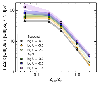
Figure 7: ($2.2\times$[O iii]88 $\mu$m$+$ [O iii]52 $\mu$m)/[N iii]57 $\mu$m ratio as a function of the gas-phase metallicity. Filled circles (squares) mark the median ratio for a given value of $U$ for the starburst (AGN) models. The shaded regions indicate the range of ratios for models with the same ionization parameter but different density.

For the metallicity diagnostics, the predicted [O iii]52 $\mu$m/[N iii]57 $\mu$m and [O iii]88 $\mu$m/[N iii]57 $\mu$m ratios, as well as the combined ($2.2\times$[O iii]88 $\mu$m$+$ [O iii]52 $\mu$m)/[N iii]57 $\mu$m ratio, have similar values (within $\sim$0.1 dex for a given $U$ and within $\sim$0.3 dex if the whole $U$ range is considered) for both the AGN and starburst models (see Figure 7). Therefore, these ratios provide robust estimates of the O⁺⁺ to N⁺⁺ abundance ratio almost independent of the ionizing spectrum, which can be used to trace the gas metallicity (see Section 3.3.1).

Finally, the [O iii]/[N ii] ratios are very dependent on $U$ as discussed in Section 3.3.2. In addition, in the case of AGN, the [N ii] transitions can be produced in XDRs (Section 3.5.1) which might not be directly connected with the ionized gas where the [O iii] originates. Consequently, the [O iii] to [N ii] ratios can only be used to measure metallicities in galaxies without an important AGN contribution or in cases where it is possible to accurately characterize the density of the gas, the properties of the radiation field ($U$ and $\alpha_{\rm AGN}$), and the XDR contribution (see also Section 3.5.3).

3.5.3 AGN power-law index

We have discussed the results for models assuming an average power-law index for the ionizing spectrum of the AGN ($\alpha_{\rm AGN}=-1.4$). However, the power-law index is known to vary (e.g., Moloney & Shull 2014). To evaluate the effect of different power-law indices, we produced models with $\alpha_{\rm AGN}$ between $-2.5$ and $-0.5$ for solar metallicity (see Section 2.2).

For the density and $U$ diagnostics, the effects of changing $\alpha_{\rm AGN}$ are similar to those described in Section 3.5.2. The scatter is increased for the density diagnostics and for the $U$ diagnostics, the XDR contribution to the Ne transitions is again the main source of uncertainty.

On the contrary, the metallicity diagnostic diagrams combining [O iii] and [N iii] transitions are almost unaffected by changes in $\alpha_{\rm AGN}$. In Figure 8, we plot the combined [O iii] to [N iii] ratio which shows a constant value independent of $\alpha_{\rm AGN}$. This is because, as discussed in Section 3.3.1, O⁺⁺ and N⁺⁺ have similar distributions in the ionized gas. Finally, diagnostics using [N ii] transitions are very sensitive to both the density and the detailed properties of the radiation field ($U$ and $\alpha_{\rm AGN}$), so they can only be used when a good knowledge of these parameters is available.

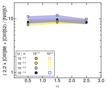
Figure 8: ($2.2\times$[O iii]88 $\mu$m$+$ [O iii]52 $\mu$m)/[N iii]57 $\mu$m ratio as a function of $\alpha_{\rm AGN}$ for solar metallicity. The symbols are as in Figure 4.

4 Application to local ULIRGs

In this section, we describe our sample of local ULIRGs observed with Herschel and apply the diagnostics described in Section 3.

4.1 Sample of local ULIRGs

We selected a sample of local ULIRGs based on the observations available in the Herschel science archive. All the galaxies in the sample were observed as part of two programs: the Herschel ULIRG Reference Survey (HERUS; Farrah et al. 2013; Spoon et al. 2013; Efstathiou et al. 2014; Pearson et al. 2016) and the Survey with Herschel of the ISM in Nearby INfrared Galaxies (SHINING; Sturm et al. 2011). For our analysis, we selected objects dominated by SF as the AGN affects some of the far-IR line ratios discussed earlier. To quantify the AGN contribution, we used the mid-IR [Ne v]14.3 $\mu$m/[Ne ii]12.8 $\mu$m ratio and included all the galaxies with a measured ratio (or upper limit) lower than 0.1, which corresponds to an AGN contribution $<$10% (Sturm et al. 2002). Using the Spitzer/IRS mid-IR spectroscopy available for these objects (Farrah et al. 2007; Inami et al. 2013), we find 19 ULIRGs that fulfill this selection criterion. Six of them are classified as Seyfert and to ensure that they are not dominated by the AGN, we search in the literature for alternative estimations of the AGN contribution. For 3 objects, we find reported AGN contributions $>$10%: IRAS 08572+3915 $>70\%$ (Veilleux et al. 2009; Nardini et al. 2010; Efstathiou et al. 2014; Hernán-Caballero et al. 2015); IRAS 15462–0450 $>20\%$ (Veilleux et al. 2009; Nardini et al. 2010); and IRAS 19254–7245 $>20\%$ (Braito et al. 2009; Nardini et al. 2010). For IRAS 13120–5453, IRAS 23128–5919, and IRAS 23253–5415, Sturm et al. (2011) and Nardini et al. (2010) report AGN contributions $<$10%, respectively. After removing the 3 Sy ULIRGs with a high AGN contribution, we define a sample with 19 ULIRGs (10 from HERUS and 9 from SHINING) listed in Table 1.

Table 1: Sample of local ULIRGs

Name	$z$	${\log L_{\rm IR}/L_{\odot}}^{a}$	Typeb	$\frac{{\rm[Ne\,V]14.3}}{[{\rm Ne\,II}]12.8}^{c}$	$\frac{{\rm[Ne\,III]15.6}}{[{\rm Ne\,II}]12.8}^{c}$	$\frac{{\rm[S\,IV]10.5}}{[{\rm Ne\,III}]15.6}^{c}$	Programd
IRAS 00188–0856	0.128	12.39	LINER	$<$0.04	0.15 $\pm$ 0.03	$<$0.38	H
IRAS 00397–1312	0.262	12.90	HII	$<$0.05	0.6 $\pm$ 0.1	0.11 $\pm$ 0.03	H
IRAS 01003–2238	0.118	12.32	HII	$<$0.10	0.42 $\pm$ 0.06	0.16 $\pm$ 0.03	H
IRAS 06035–7102	0.079	12.22	HII	$<$0.07	0.25 $\pm$ 0.05	$<$0.22	H
IRAS 10565+2448	0.043	12.28	HII	$<$0.02	0.12 $\pm$ 0.02	$<$0.04	S
IRAS 11095–0238	0.107	12.28	LINER	$<$0.08	0.31 $\pm$ 0.04	$<$0.63	H
IRASF 12112+0305	0.073	12.48	LINER	$<$0.05	0.22 $\pm$ 0.02	0.21 $\pm$ 0.04	S
IRAS 13120–5453	0.031	12.47	Sy2	0.011 $\pm$ 0.002	0.12 $\pm$ 0.02	0.027 $\pm$ 0.006	S
IRAS 14348–1447	0.083	12.60	LINER	$<$0.02	0.24 $\pm$ 0.03	0.10 $\pm$ 0.03	S
IRAS 16090–0139	0.134	12.55	LINER	$<$0.02	0.26 $\pm$ 0.04	$<$0.10	H
IRAS 17208–0014	0.043	12.68	HII	$<$0.02	0.20 $\pm$ 0.03	$<$0.05	S
IRAS 19297–0406	0.086	12.61	HII	$<$0.05	0.14 $\pm$ 0.02	$<$0.16	S
IRAS 20087–0308	0.106	12.42	LINER	$<$0.05	0.12 $\pm$ 0.01	$<$0.29	H
IRAS 20100–4156	0.130	12.67	HII	$<$0.07	0.4 $\pm$ 0.1	$<$0.07	H
IRAS 20551–4250	0.043	12.24	HII	$<$0.06	0.21 $\pm$ 0.03	$<$0.14	S
IRAS 23128–5919	0.045	12.21	Sy2	0.09 $\pm$ 0.01	0.7 $\pm$ 0.1	0.22 $\pm$ 0.03	S
IRAS 23230–6926	0.106	12.37	LINER	$<$0.10	0.27 $\pm$ 0.02	$<$0.36	H
IRAS 23253–5415	0.130	12.36	Sy2	0.06 $\pm$ 0.02	0.34 $\pm$ 0.05	0.57 $\pm$ 0.09	H
IRAS 23365+3604	0.064	12.37	LINER	$<$0.09	0.09 $\pm$ 0.01	$<$1.03	S

Notes: ^(a) Total 8–1000 $\mu$m IR luminosity from De Looze et al. (2014). ^(b) Nuclear activity classification from the NASA Extragalactic Database. ^(c) Mid-IR line ratios from Spitzer/IRS spectroscopy from Farrah et al. (2007) for all the galaxies except for IRASF 12112+0305 (Inami et al. 2013). ^(d). Herschel program that observed each object. H stands for HERUS (Farrah et al. 2013) and S for SHINING (Sturm et al. 2011). For the non detections, we state the 3$\sigma$ upper limits.

Table 2: Far-IR line emission fluxes

Name	[O iii]52 $\mu$m	[N iii]57 $\mu$m	[O i]63 $\mu$m	[O iii]88 $\mu$m	[N ii]122 $\mu$m	[O i]146 $\mu$m	[C ii]158 $\mu$m	[N ii]205 $\mu$ma
00188–0856b	$<$0.24	$<$0.16	$<$0.21	$\cdots$	$<$0.15	$<$0.12	$<$0.3	0.043 $\pm$ 0.007
00397–1312b	0.30 $\pm$ 0.04	$<$0.09	0.50 $\pm$ 0.05	$\cdots$	$<$0.027	$<$0.027	0.16 $\pm$ 0.02	$<$0.024
01003–2238b	$<$0.30	$<$0.09	0.9 $\pm$ 0.2	$\cdots$	$<$0.05	$<$0.04	$<$0.4	$\cdots$
06035–7102b	$<$3	$<$1.3	$<$2.3	$\cdots$	$<$0.18	$<$0.21	3.1 $\pm$ 0.2	$<$0.028
10565+2448	$\cdots$	0.91 $\pm$ 0.04	6.74 $\pm$ 0.07	1.56 $\pm$ 0.04	$\cdots$	0.51 $\pm$ 0.03	5.88 $\pm$ 0.04	0.24 $\pm$ 0.01
11095–0238b	$<$0.4	$<$0.25	0.9 $\pm$ 0.1	$\cdots$	0.063 $\pm$ 0.009	$<$0.16	0.8 $\pm$ 0.1	0.048 $\pm$ 0.008
12112+0305	$\cdots$	0.56 $\pm$ 0.09	0.8 $\pm$ 0.1	0.74 $\pm$ 0.05	$\cdots$	0.20 $\pm$ 0.01	2.34 $\pm$ 0.05	$\cdots$
13120–5453	$\cdots$	2.2 $\pm$ 0.2	14.1 $\pm$ 0.2	2.61 $\pm$ 0.08	$\cdots$	1.28 $\pm$ 0.05	12.88 $\pm$ 0.06	0.64 $\pm$ 0.02
14348–1447	$\cdots$	$\cdots$	2.43 $\pm$ 0.09	0.67 $\pm$ 0.02	$\cdots$	0.22 $\pm$ 0.02	2.78 $\pm$ 0.03	0.11 $\pm$ 0.01
16090–0139b	$<$1.6	$<$0.9	$<$2.5	$\cdots$	0.10 $\pm$ 0.01	$<$0.20	1.0 $\pm$ 0.1	0.043 $\pm$ 0.008
17208–0014	$\cdots$	2.0 $\pm$ 0.2	3.2 $\pm$ 0.1	3.1 $\pm$ 0.1	$\cdots$	0.66 $\pm$ 0.05	8.61 $\pm$ 0.05	0.32 $\pm$ 0.02
19297–0406	$\cdots$	$<$0.4	2.15 $\pm$ 0.09	0.55 $\pm$ 0.05	$\cdots$	0.22 $\pm$ 0.03	2.69 $\pm$ 0.05	$<$0.03
20087–0308b	$<$3	$<$1.6	0.6 $\pm$ 0.1	$\cdots$	0.235 $\pm$ 0.010	$<$0.22	1.71 $\pm$ 0.02	0.053 $\pm$ 0.009
20100–4156b	0.49 $\pm$ 0.08	$<$0.13	0.80 $\pm$ 0.08	$\cdots$	0.092 $\pm$ 0.008	0.096 $\pm$ 0.010	0.96 $\pm$ 0.02	0.076 $\pm$ 0.010
20551–4250	$\cdots$	0.40 $\pm$ 0.07	4.11 $\pm$ 0.06	1.31 $\pm$ 0.04	$\cdots$	0.47 $\pm$ 0.04	4.42 $\pm$ 0.03	0.08 $\pm$ 0.01
23128–5919	$\cdots$	1.71 $\pm$ 0.09	6.8 $\pm$ 0.1	4.44 $\pm$ 0.07	$\cdots$	0.64 $\pm$ 0.05	6.27 $\pm$ 0.04	0.183 $\pm$ 0.010
23230–6926b	$<$0.27	$<$0.23	0.6 $\pm$ 0.1	$\cdots$	0.09 $\pm$ 0.01	0.13 $\pm$ 0.01	1.00 $\pm$ 0.02	$<$0.023
23253–5415b	$<$0.23	$<$0.16	$<$1.7	$\cdots$	0.08 $\pm$ 0.01	$<$0.04	1.3 $\pm$ 0.1	0.048 $\pm$ 0.008
23365+3604	$\cdots$	$\cdots$	1.91 $\pm$ 0.07	0.47 $\pm$ 0.03	$\cdots$	0.19 $\pm$ 0.01	1.87 $\pm$ 0.04	0.09 $\pm$ 0.01

Notes: Fluxes are in units of 10^-13 erg cm^-2 s^-1. ^(a) The [N ii]205 $\mu$m flux is from the Herschel/SPIRE FTS (Griffin et al. 2010) data available for these objects (Pearson et al. 2016). ^(b) For the HERUS sources, we use the fluxes published by Farrah et al. (2013). For the non detections, we state the 3$\sigma$ upper limits.

4.2 Herschel/PACS data

The brightest far-IR fine-structure emission lines of our sample of local ULIRGs were observed with Herschel/PACS (Poglitsch et al. 2010). PACS contains an integral field spectrograph which covers a field of view of 47″$\times$47″with 5$\times$5 square pixels with a side of 9$\aas@@fstack{\prime\prime}$4. For the HERUS galaxies, we used the PACS fluxes already published by Farrah et al. (2013). For the SHINING objects, we downloaded the data from the archive and used the PACSman package (Lebouteiller et al. 2012) to obtain the fully reduced and calibrated data cubes.

The SHINING sources are point-like at the angular resolution of PACS. Therefore, we extracted the spectrum of the central spaxel and applied the point source loss correction factor provided in the PACS calibration set. We also extracted the spectra form the central 3$\times$3 spaxels and applied the corresponding point source correction. The fluxes using these two apertures are compatible, which confirms that the emission of these objects is not resolved by PACS and that the source is well centered within the central spaxel. In the following, we use only the spectra from the central spaxel, since the signal-to-noise ratio is higher than in the 3$\times$3 spaxels spectra.

In Figure 9, we plot the continuum subtracted emission line profiles which, in most cases, deviate from a simple Gaussian profile. For this reason, to measure the line fluxes, we integrated all the spectral channels in the velocity range where we detect [C ii]158 $\mu$m emission (the brightest of these transitions) at more than 3$\sigma$ (about $\pm$500 km s^-1). The measured fluxes are listed in Table 2 together with the fluxes of the HERUS objects from Farrah et al. (2013). The [O i]63 $\mu$m transitions is sometimes affected by self-absorption. This is clear in the spectrum of IRASF 17208-0014. We do not attempt to correct for this absorption, therefore, the [O i]63 $\mu$m fluxes reported in Table 2 should be considered as lower limits of the total [O i]63 $\mu$m emission.

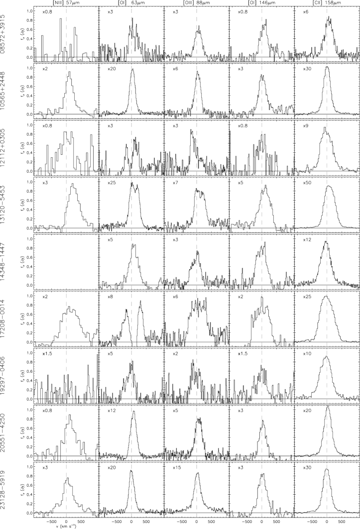
Figure 9: Continuum subtracted far-IR transitions observed by Herschel/PACS for the SHINING ULIRGs in our sample. The spectra are scaled by the factor indicated in each panel. The vertical dashed line marks the systemic velocity of each object based on the reported redshift in Table 1.

4.3 IR diagnostics

4.3.1 Gas density

Farrah et al. (2007) and Inami et al. (2013) presented the [S iii] fluxes for 11 objects in our sample of local ULIRGs. The [S iii]19 $\mu$m/[S iii]33 $\mu$m ratios range between 0.30 and 1.1 with a median ratio of 0.48. This median ratio corresponds to a density of 10^2.1 cm^-3 (Figure 1). For 5 objects, the [N ii]122 $\mu$m and [N ii]205 $\mu$m fluxes are published by Farrah et al. (2013) and Pearson et al. (2016), respectively. We measure [N ii]122 $\mu$m/[N ii]205 $\mu$m ratios between 1.2 and 4.4 and the median ratio equals to 1.7. The median ratio corresponds to gas densities in the range 10^1.3-1.6 cm^-3 (Figure 1). None of these ULIRGs were observed in both far-IR [O iii] transitions, so we cannot use this ratio to constrain the density.

The density derived from the [N ii] ratio is slightly lower than that derived from the [S iii] ratio. A similar result was found by Fernández-Ontiveros et al. (2016) and Spinoglio et al. (2015) when comparing gas densities derived from these two pairs of transitions. This might indicate that the density structure of SF regions is more complex than the constant pressure model assumed in Section 2. For simplicity, we adopt a single gas density value of $\sim$10² cm^-3, intermediate between the [S iii] and [N ii] derived values, as a representative value for local starburst dominated ULIRGs. We limit our discussion to models with $n_{\rm H}\leq 10^{4}$ cm^-3 to match the observed range of densities in these local ULIRGs.

4.3.2 Ionization parameter

We calculate the [S iv]11 $\mu$m/[Ne iii]16 $\mu$m ratio for 7 ULIRGs (see Table 1). This ratio ranges from 0.03 to 0.57. Since most of the galaxies have upper limits for this ratio, we performed a survival analysis on the data. We used the Kaplan-Meier estimator (see Feigelson & Nelson 1985) obtaining a mean ratio of 0.11$\pm$0.04. This ratio is consistent with an ionization parameter, $\log U$, between –3.0 and –2.3.

In Figure 3, we also plot the observed [Ne ii]13 $\mu$m/[Ne iii]16 $\mu$m ratio range in our sample of ULIRGs. It corresponds to $\log\,U>-2.7$ assuming $Z_{\rm gas}>0.5$$Z_{\rm\odot}$, which agrees with the $U$ derived using the [S iv]11 $\mu$m/[Ne iii]16 $\mu$m ratio.

4.3.3 Metallicity

None of our objects have simultaneous observations of the two [O iii] transitions. The SHINING objects have [O iii]88 $\mu$m observations and the HERUS objects [O iii]52 $\mu$m observations. Therefore, we cannot use the combined [O iii] ratio diagram. Instead, for 6 SHINING objects, we measure both the [O iii]88 and [N iii]57 $\mu$m transitions (Table 2), so we can use the [O iii]88 $\mu$m/[N iii]57 $\mu$m ratio to estimate the gas metallicity. In these objects, this ratio ranges from 1.2 to 3.3 with a median ratio of 1.6. For the average gas density, $n_{\rm H}=10^{2}$ cm^-3, derived in Section 4.3.1, the observed range in this ratio corresponds to metallicities between 0.7 and 1.5 $Z_{\rm\odot}$ (Figure LABEL:fig:o3_n3). For the two HERUS galaxies where the [O iii]52 $\mu$m transition is detected, the [N iii]57 $\mu$m is not. But using the [N iii]57 $\mu$m upper limits, we estimate that the [O iii]52 $\mu$m/[N iii]57 $\mu$m ratio is $>$3. This constrains the $Z_{\rm gas}$ to be $<$0.6–0.8 $Z_{\rm\odot}$ (for $n_{\rm H}=10^{2}$ cm^-3), which is consistent with the lower end of the metallicity range derived for the SHINING ULIRGs.

In our sample of ULIRGs, we measured the [O iii]88 $\mu$m/[N ii]205 $\mu$m ratio in 7 objects. This ratio ranges from 4 to 24 with a median value of 7. In left panel of Figure LABEL:fig:Z_o3, we show that these values correspond to a metallicity range about $\sim$0.8–2.0$Z_{\rm\odot}$ (assuming $\log U=$–2.5 and –3.0 and $n_{\rm H}\sim 10^{2}$ cm^-3, Sections 4.3.1 and 4.3.2) which is compatible with the range obtained using the [O iii]/[N iii]57 $\mu$m ratios.

It is also worth noting that the [N ii]205 $\mu$m/[C ii]158 $\mu$m ratio has been used to estimate metallicities in high-$z$ galaxies (e.g., Nagao et al. 2012; Béthermin et al. 2016). However, we do not consider this ratio in our work for two reasons: (i) the [C ii]158 $\mu$m emission is produced in both H ii regions and in photodissociation regions (PDR) and the proper estimation of the [C ii]158 $\mu$m PDR emission is beyond the scope of this work. In addition, the [N ii]205 $\mu$m/[C ii]158 $\mu$m ratio has been used to determine the fraction of [C ii]158 $\mu$m emission produced by H ii regions (e.g., Oberst et al. 2006), although this determination relies on the modeling of the ionization structure of the H ii region and the assumed abundances of C and N; and (ii) C is a “pseudo-secondary” element (Henry et al. 2000), so its abundance does not exactly follow that of primary elements. Actually, several works (e.g., Garnett et al. 1999; Berg et al. 2016) found that the C/N abundance ratio is approximately constant for a wide range of O/H values. Therefore, ratios using C and N transitions might produce uncertain estimates of the metallicity unless a careful modeling is performed.

4.3.4 Comparison with optical metallicity determination

Optical line ratios have been used to measure metallicities in local ULIRGs in the past (e.g., Rupke et al. 2008; Kilerci Eser et al. 2014). These works use strong-line techniques to determine the oxygen abundance (e.g., Pagel et al. 1979) using various optical ratios and calibrations. In particular, both works made use of the $R_{23}$ ratio adopting the Tremonti et al. (2004) calibration, so for the comparison here, we only consider their results obtained with this calibration. We note that they corrected the line fluxes for extinction using the observed Balmer decrement. Rupke et al. (2008) and Kilerci Eser et al. (2014) find that local ULIRGs have oxygen abundances 12+$\log{\rm(O/H)}=$ 8.6$\pm$0.2 and 8.7$\pm$0.2 for samples with 25 and 47 ULIRGs, respectively. These values correspond to a solar O abundance (Asplund et al. 2009). Using the far-IR line ratios, we find that $0.7<Z_{\rm gas}/$$Z_{\rm\odot}$$<1.5$, which corresponds to $8.5<12+\log({\rm O/H})<8.9$, so the range derived from the far-IR agrees well with the range observed using this optical metallicity indicator.

However, different optical metallicity diagnostics produce systematically different absolute $12+\log({\rm O/H})$ values (see Kewley & Ellison 2008 and figure 2 of Rupke et al. 2008). Therefore, the agreement between the metallicity ranges derived using far-IR and optical lines applies only to the $R_{23}$ method using the Tremonti et al. (2004) calibration, although it is possible to apply conversion factors between different calibrations (Kewley & Ellison 2008).

Previous works have shown that ULIRGs lie below the mass-metallicity relation followed by normal star-forming galaxies (e.g., Rupke et al. 2008; Caputi et al. 2008; Kilerci Eser et al. 2014). To test this result using the metallicity derived here, we need an estimate for the stellar mass of our ULIRGs. We found dynamical masses for 14 objects ($\sim$70% of the sample) in the literature (Dasyra et al. 2006a, b; Tacconi et al. 2002; Genzel et al. 2001). They range from 10¹⁰ $M_{\rm\odot}$ to 2$\times 10^{11}$ $M_{\rm\odot}$, with a median dynamical mass of (5$\pm$2)$\times 10^{10}$ $M_{\rm\odot}$. Stellar masses in ULIRGs are lower than the dynamical masses, but typically they are within a factor of 2 (Rodríguez Zaurín et al. 2010). Taking this into account, we estimate an average stellar mass of 2 to 7$\times 10^{10}$ $M_{\rm\odot}$. For this range of masses, according to the mass-metallicity relation (Tremonti et al. 2004), the expected metalilcity is $12+\log({\rm O/H})=8.94-9.15$. That is, the expected average metallicity is a factor of 2 higher than the value we derive using the far-IR diagnostics. Therefore, our findings are consistent with the results obtained by previous works using optical metallicity diagnostics.

5 Conclusions

We used the photoinization code cloudy to model the fine-structure far-IR emission lines present in the spectra of galaxies. We focus on the far-IR line ratios that can be used to determine the gas-phase metallicity and apply our models to a sample of local ULIRGs observed with Herschel and Spitzer. We also explore the effect of an AGN on these ratios. The main results of this work are as follows:

1. We find that the best far-IR ratios to estimate gas metallicities are those using the far-IR [O iii]52 $\mu$m and 88 $\mu$m to [N iii]57 $\mu$m ratios as previously shown by Nagao et al. (2011). In particular, we find that the best estimate for the metallicity is obtained with following ratio ($2.2\times$[O iii]88 $\mu$m$+$ [O iii]52 $\mu$m)/[N iii]57 $\mu$m which reduces the scatter due to variations in the gas density and ionization parameter to 0.2 dex. We find that these ratios are not significantly affected by the SF history (age of the ionizing stellar population) or by the presence of an AGN. Therefore, they can provide robust metallicity estimates independently of the ionizing source and the ionization parameter.

2. For high-$z$ objects, we explore the [O iii]52 $\mu$m and 88 $\mu$m to [N ii]122 $\mu$m and [N ii]205 $\mu$m ratios. The best combination is the [O iii]88 $\mu$m/[N ii]122 $\mu$m ratio since both transitions have similar critical densities and can be observed at $z\gtrsim 3$ with ALMA. We caution that these ratios involving [O iii] and [N ii] transitions have a strong dependence on the ionization parameter which should be estimated using different line ratios. Although, the [O iii] to [N ii] ratios are sensitive to the age of the ionizing stellar population, they can provide rough metallicity estimates even in situations where a constant SF history does not apply. On the other hand, these ratios are highly affected by the AGN radiation since the [N ii] lines can be significantly produced in XDRs.

3. To estimate the gas density, we use typical ratios between pairs of transitions of the same ion, while to estimate the ionization parameter $U$, we propose the [S iv]11 $\mu$m/[Ne iii]16 $\mu$m ratio. Other ratios like the [Ne ii]13 $\mu$m/[Ne iii]16 $\mu$m, [N ii]122 $\mu$m/[N iii]57 $\mu$m, or [O iii]88 $\mu$m/[N ii]122 $\mu$m can be used to derive $U$ if a rough estimate of the metallicity is available.

4. We apply these ratios to a sample of 19 local ULIRGs and obtain a gas density $\sim$10² cm^-3 and an ionization parameter $\log\,U$ between –3.0 and –2.3. Using the metallicity diagnostics described above, we estimate that the gas-phase metallicity in these local ULIRGs is $0.7<Z_{\rm gas}/$$Z_{\rm\odot}$$<1.5$, which correspond to $8.5<12+\log({\rm O/H})<8.9$ for the assumed solar chemical composition (Asplund et al. 2009). This range agrees with the metallicity range observed in local ULIRGs using optical line ratios and this confirms the decreased metallicity in local ULIRGs with respect to the local mass-metallicity relation.

Appendix A Predicted line ratios for starburst models

In Table LABEL:tbl:sb_models, we present the numerical values of the line ratios predicted by the continuous starburst cloudy models (Section 2.1) as a function of the metallicity $Z$, the gas volume density $\log n_{\rm H}$, and the ionization parameter $\log U$.

Table 3: Logarithm of the mid- and far-IR line ratios for the starburst models

$Z/Z_{\odot}$	$\log\frac{n_{\rm H}}{{\rm cm^{-3}}}$	$\log\,U$	$\frac{{\rm[S\,{\scriptscriptstyle III}]19}}{{\rm[S\,{\scriptscriptstyle III}]33}}$	$\frac{{\rm[O\,{\scriptscriptstyle III}]52}}{{\rm[O\,{\scriptscriptstyle III}]88}}$	$\frac{{\rm[N\,{\scriptscriptstyle II}]122}}{{\rm[N\,{\scriptscriptstyle II}]205}}$	$\frac{{\rm[S\,{\scriptscriptstyle IV}]11}}{{\rm[Ne\,{\scriptscriptstyle III}]16}}$	$\frac{{\rm[Ne\,{\scriptscriptstyle II}]13}}{{\rm[Ne\,{\scriptscriptstyle III}]16}}$	$\frac{{\rm[O\,{\scriptscriptstyle III}]52}}{{\rm[N\,{\scriptscriptstyle III}]57}}$	$\frac{{\rm[O\,{\scriptscriptstyle III}]88}}{{\rm[N\,{\scriptscriptstyle III}]57}}$	$\frac{{\rm[O\,{\scriptscriptstyle III}]52}}{{\rm[N\,{\scriptscriptstyle II}]122}}$	$\frac{{\rm[O\,{\scriptscriptstyle III}]52}}{{\rm[N\,{\scriptscriptstyle II}]205}}$	$\frac{{\rm[O\,{\scriptscriptstyle III}]88}}{{\rm[N\,{\scriptscriptstyle II}]122}}$	$\frac{{\rm[O\,{\scriptscriptstyle III}]88}}{{\rm[N\,{\scriptscriptstyle II}]205}}$
0.05	1	–4.0	–0.36	–0.23	–0.04	–2.49	0.30	0.97	1.20	0.10	0.06	0.33	0.29
0.05	1	–3.5	–0.35	–0.23	–0.04	–1.66	–0.19	1.00	1.23	1.05	1.01	1.28	1.24
0.05	1	–3.0	–0.34	–0.23	–0.03	–0.95	–0.69	1.07	1.30	1.88	1.84	2.11	2.07
0.05	1	–2.5	–0.33	–0.23	–0.02	–0.36	–1.19	1.12	1.35	2.50	2.48	2.73	2.70
0.05	1	–2.0	–0.32	–0.23	–0.01	0.09	–1.69	1.17	1.40	3.01	3.00	3.24	3.22
0.05	2	–4.0	–0.29	–0.10	0.43	–2.48	0.31	1.06	1.16	0.25	0.68	0.35	0.78
0.05	2	–3.5	–0.28	–0.10	0.44	–1.66	–0.18	1.09	1.19	1.21	1.65	1.30	1.75
0.05	2	–3.0	–0.27	–0.10	0.45	–0.95	–0.68	1.16	1.26	2.04	2.49	2.14	2.59
0.05	2	–2.5	–0.27	–0.10	0.46	–0.36	–1.19	1.21	1.31	2.67	3.12	2.76	3.22
0.05	2	–2.0	–0.26	–0.09	0.47	0.09	–1.69	1.26	1.35	3.18	3.65	3.27	3.74
0.05	3	–4.0	0.07	0.40	0.86	–2.49	0.31	1.36	0.97	0.80	1.66	0.41	1.26
0.05	3	–3.5	0.08	0.40	0.87	–1.67	–0.18	1.40	1.00	1.77	2.63	1.37	2.24
0.05	3	–3.0	0.08	0.39	0.87	–0.95	–0.68	1.47	1.08	2.60	3.47	2.21	3.08
0.05	3	–2.5	0.07	0.39	0.86	–0.36	–1.18	1.52	1.13	3.23	4.09	2.84	3.71
0.05	3	–2.0	0.06	0.38	0.86	0.09	–1.69	1.57	1.19	3.76	4.61	3.38	4.23
0.05	4	–4.0	0.71	0.87	0.97	–2.61	0.35	1.59	0.72	1.09	2.06	0.21	1.18
0.05	4	–3.5	0.72	0.88	0.97	–1.79	–0.14	1.63	0.75	2.05	3.03	1.18	2.15
0.05	4	–3.0	0.71	0.87	0.97	–1.06	–0.65	1.70	0.83	2.90	3.87	2.02	3.00
0.05	4	–2.5	0.70	0.87	0.97	–0.46	–1.15	1.76	0.89	3.53	4.50	2.66	3.63
0.05	4	–2.0	0.68	0.86	0.97	0.00	–1.66	1.82	0.96	4.09	5.05	3.23	4.19
0.05	5	–4.0	1.02	1.00	0.99	–3.02	0.50	1.63	0.64	1.08	2.07	0.09	1.08
0.05	5	–3.5	1.03	1.00	0.99	–2.18	0.01	1.67	0.67	2.06	3.05	1.07	2.06
0.05	5	–3.0	1.03	1.00	0.99	–1.44	–0.49	1.74	0.75	2.92	3.91	1.92	2.91
0.05	5	–2.5	1.03	1.00	0.99	–0.83	–1.00	1.80	0.81	3.56	4.55	2.56	3.55
0.05	5	–2.0	1.02	1.00	0.99	–0.36	–1.52	1.87	0.87	4.12	5.11	3.13	4.12
0.05	6	–4.0	1.07	1.01	0.99	–3.29	0.77	1.64	0.63	1.06	2.05	0.05	1.04
0.05	6	–3.5	1.08	1.01	0.99	–2.42	0.28	1.67	0.66	2.05	3.04	1.03	2.03
0.05	6	–3.0	1.08	1.01	0.99	–1.67	–0.23	1.75	0.74	2.90	3.90	1.89	2.88
0.05	6	–2.5	1.08	1.01	0.99	–1.05	–0.74	1.81	0.80	3.32	4.31	2.31	3.30
0.05	6	–2.0	1.08	1.01	0.98	–0.60	–1.28	1.88	0.86	2.45	3.43	1.43	2.42
0.20	1	–4.0	–0.36	–0.23	–0.04	–2.48	0.48	0.95	1.19	–0.01	–0.05	0.22	0.18
0.20	1	–3.5	–0.35	–0.23	–0.03	–1.70	–0.00	0.99	1.22	0.93	0.89	1.16	1.13
0.20	1	–3.0	–0.35	–0.23	–0.03	–1.03	–0.50	1.06	1.29	1.78	1.74	2.01	1.97
0.20	1	–2.5	–0.35	–0.23	–0.04	–0.46	–0.99	1.12	1.35	2.44	2.40	2.67	2.63
0.20	1	–2.0	–0.34	–0.22	–0.03	–0.00	–1.47	1.16	1.38	2.97	2.94	3.19	3.16
0.20	2	–4.0	–0.29	–0.10	0.43	–2.47	0.48	1.05	1.14	0.15	0.58	0.25	0.68
0.20	2	–3.5	–0.29	–0.09	0.45	–1.70	–0.00	1.08	1.17	1.09	1.54	1.19	1.63
0.20	2	–3.0	–0.28	–0.09	0.44	–1.03	–0.50	1.15	1.24	1.94	2.38	2.03	2.47
0.20	2	–2.5	–0.28	–0.08	0.44	–0.46	–0.99	1.21	1.30	2.59	3.03	2.68	3.11
0.20	2	–2.0	–0.28	–0.06	0.44	–0.00	–1.47	1.26	1.32	3.12	3.56	3.18	3.62
0.20	3	–4.0	0.08	0.40	0.86	–2.48	0.49	1.35	0.95	0.70	1.57	0.30	1.16
0.20	3	–3.5	0.09	0.41	0.87	–1.70	0.00	1.38	0.98	1.66	2.53	1.25	2.12
0.20	3	–3.0	0.08	0.41	0.87	–1.04	–0.49	1.46	1.05	2.49	3.36	2.09	2.96
0.20	3	–2.5	0.08	0.41	0.86	–0.46	–0.99	1.51	1.11	3.14	4.00	2.73	3.59
0.20	3	–2.0	0.08	0.42	0.85	–0.00	–1.47	1.55	1.13	3.65	4.51	3.23	4.09
0.20	4	–4.0	0.71	0.88	0.97	–2.60	0.53	1.57	0.69	0.99	1.96	0.11	1.09
0.20	4	–3.5	0.72	0.88	0.98	–1.83	0.04	1.60	0.72	1.95	2.92	1.07	2.05
0.20	4	–3.0	0.72	0.88	0.98	–1.16	–0.46	1.68	0.81	2.79	3.77	1.92	2.89
0.20	4	–2.5	0.72	0.87	0.97	–0.58	–0.96	1.74	0.87	3.44	4.41	2.56	3.54
0.20	4	–2.0	0.72	0.87	0.97	–0.12	–1.44	1.78	0.91	3.95	4.92	3.08	4.05
0.20	5	–4.0	1.02	1.00	0.99	–3.01	0.68	1.61	0.61	0.99	1.99	–0.00	0.99
0.20	5	–3.5	1.03	1.00	0.99	–2.22	0.19	1.64	0.64	1.97	2.96	0.97	1.96
0.20	5	–3.0	1.03	1.00	0.99	–1.54	–0.31	1.72	0.73	2.82	3.81	1.82	2.81
0.20	5	–2.5	1.03	1.00	0.97	–0.96	–0.81	1.79	0.79	3.16	4.13	2.16	3.13
0.20	5	–2.0	1.03	1.00	0.96	–0.51	–1.29	1.83	0.83	3.09	4.05	2.09	3.05
0.20	6	–4.0	1.07	1.01	0.99	–3.27	0.94	1.61	0.60	0.97	1.96	–0.04	0.95
0.20	6	–3.5	1.08	1.01	0.99	–2.46	0.46	1.64	0.63	1.92	2.92	0.91	1.90
0.20	6	–3.0	1.08	1.01	0.99	–1.76	–0.05	1.73	0.71	2.38	3.37	1.37	2.36
0.20	6	–2.5	1.08	1.01	0.98	–1.17	–0.56	1.79	0.78	2.53	3.52	1.52	2.51
0.20	6	–2.0	1.08	1.01	0.99	–0.72	–1.05	1.84	0.83	2.62	3.60	1.60	2.59
0.40	1	–4.0	–0.37	–0.23	–0.04	–2.49	0.58	0.67	0.90	–0.38	–0.42	–0.15	–0.19
0.40	1	–3.5	–0.37	–0.23	–0.03	–1.73	0.11	0.70	0.93	0.54	0.51	0.77	0.74
0.40	1	–3.0	–0.37	–0.23	–0.03	–1.08	–0.37	0.76	1.00	1.38	1.35	1.61	1.58
0.40	1	–2.5	–0.37	–0.23	–0.04	–0.52	–0.84	0.82	1.05	2.04	2.00	2.27	2.23
0.40	1	–2.0	–0.37	–0.22	–0.03	–0.07	–1.28	0.86	1.08	2.55	2.52	2.77	2.74
0.40	2	–4.0	–0.30	–0.09	0.44	–2.48	0.58	0.76	0.85	–0.22	0.22	–0.13	0.31
0.40	2	–3.5	–0.29	–0.09	0.45	–1.72	0.11	0.79	0.88	0.71	1.16	0.80	1.25
0.40	2	–3.0	–0.29	–0.08	0.45	–1.07	–0.37	0.86	0.94	1.55	1.99	1.63	2.08
0.40	2	–2.5	–0.29	–0.07	0.44	–0.52	–0.84	0.92	0.99	2.20	2.64	2.27	2.70
0.40	2	–2.0	–0.28	–0.02	0.45	–0.07	–1.28	0.96	0.99	2.72	3.17	2.74	3.19
0.40	3	–4.0	0.09	0.41	0.87	–2.49	0.59	1.06	0.65	0.34	1.20	–0.07	0.79
0.40	3	–3.5	0.10	0.42	0.87	–1.73	0.12	1.10	0.68	1.28	2.15	0.86	1.73
0.40	3	–3.0	0.10	0.42	0.87	–1.08	–0.37	1.16	0.74	2.10	2.97	1.68	2.55
0.40	3	–2.5	0.10	0.43	0.86	–0.52	–0.84	1.22	0.78	2.74	3.60	2.31	3.17
0.40	3	–2.0	0.12	0.46	0.86	–0.08	–1.29	1.25	0.79	3.24	4.10	2.77	3.64
0.40	4	–4.0	0.72	0.88	0.98	–2.61	0.62	1.27	0.39	0.63	1.60	–0.25	0.73
0.40	4	–3.5	0.73	0.88	0.98	–1.86	0.15	1.30	0.42	1.57	2.55	0.69	1.67
0.40	4	–3.0	0.73	0.88	0.98	–1.21	–0.34	1.38	0.49	2.40	3.38	1.52	2.50
0.40	4	–2.5	0.73	0.88	0.97	–0.65	–0.82	1.43	0.55	3.03	4.00	2.15	3.12
0.40	4	–2.0	0.75	0.88	0.95	–0.22	–1.26	1.46	0.58	3.42	4.38	2.54	3.50
0.40	5	–4.0	1.02	1.00	0.99	–3.02	0.77	1.30	0.31	0.64	1.64	–0.35	0.64
0.40	5	–3.5	1.03	1.00	0.99	–2.25	0.30	1.33	0.34	1.60	2.59	0.60	1.59
0.40	5	–3.0	1.03	1.00	0.98	–1.60	–0.19	1.41	0.42	2.36	3.35	1.37	2.35
0.40	5	–2.5	1.03	1.00	0.97	–1.05	–0.67	1.47	0.48	2.66	3.62	1.66	2.63
0.40	5	–2.0	1.03	1.00	0.96	–0.61	–1.10	1.51	0.51	2.75	3.71	1.75	2.72
0.40	6	–4.0	1.07	1.01	0.99	–3.28	1.04	1.30	0.29	0.62	1.61	–0.39	0.60
0.40	6	–3.5	1.07	1.01	0.99	–2.48	0.56	1.33	0.32	1.47	2.46	0.46	1.45
0.40	6	–3.0	1.08	1.01	0.99	–1.82	0.06	1.41	0.40	2.03	3.02	1.02	2.01
0.40	6	–2.5	1.08	1.01	0.99	–1.26	–0.42	1.48	0.47	2.33	3.32	1.32	2.31
0.40	6	–2.0	1.08	1.01	0.99	–0.81	–0.87	1.52	0.50	2.56	3.55	1.55	2.54
1.00	1	–4.0	–0.40	–0.24	–0.02	–2.42	1.11	0.05	0.29	–1.31	–1.33	–1.07	–1.09
1.00	1	–3.5	–0.40	–0.24	–0.01	–1.71	0.67	0.07	0.30	–0.41	–0.42	–0.17	–0.18
1.00	1	–3.0	–0.40	–0.24	–0.01	–1.14	0.23	0.12	0.35	0.41	0.41	0.65	0.64
1.00	1	–2.5	–0.41	–0.23	–0.01	–0.71	–0.18	0.19	0.43	1.07	1.06	1.30	1.30
1.00	1	–2.0	–0.41	–0.21	0.02	–0.36	–0.53	0.25	0.46	1.52	1.55	1.73	1.76
1.00	2	–4.0	–0.31	–0.08	0.47	–2.41	1.11	0.14	0.23	–1.12	–0.65	–1.04	–0.57
1.00	2	–3.5	–0.30	–0.07	0.49	–1.70	0.67	0.17	0.24	–0.21	0.28	–0.14	0.35
1.00	2	–3.0	–0.30	–0.06	0.49	–1.13	0.23	0.22	0.29	0.62	1.11	0.69	1.17
1.00	2	–2.5	–0.30	–0.03	0.49	–0.70	–0.18	0.31	0.34	1.28	1.77	1.32	1.80
1.00	2	–2.0	–0.28	0.04	0.53	–0.34	–0.55	0.38	0.34	1.78	2.31	1.74	2.27
1.00	3	–4.0	0.11	0.44	0.88	–2.41	1.11	0.44	0.00	–0.55	0.33	–0.99	–0.11
1.00	3	–3.5	0.13	0.45	0.89	–1.70	0.67	0.47	0.01	0.37	1.26	–0.08	0.81
1.00	3	–3.0	0.14	0.46	0.89	–1.14	0.23	0.52	0.06	1.20	2.10	0.74	1.63
1.00	3	–2.5	0.15	0.48	0.89	–0.70	–0.20	0.60	0.12	1.86	2.75	1.38	2.27
1.00	3	–2.0	0.20	0.52	0.90	–0.34	–0.57	0.65	0.13	2.35	3.25	1.83	2.73
1.00	4	–4.0	0.74	0.89	0.98	–2.55	1.14	0.62	–0.26	–0.26	0.72	–1.15	–0.17
1.00	4	–3.5	0.76	0.89	0.98	–1.84	0.70	0.65	–0.25	0.66	1.64	–0.24	0.75
1.00	4	–3.0	0.76	0.89	0.98	–1.28	0.25	0.71	–0.19	1.50	2.48	0.61	1.59
1.00	4	–2.5	0.77	0.89	0.98	–0.84	–0.18	0.79	–0.11	2.16	3.13	1.26	2.24
1.00	4	–2.0	0.80	0.89	0.97	–0.49	–0.56	0.83	–0.07	2.57	3.53	1.67	2.64
1.00	5	–4.0	1.02	1.00	0.99	–2.94	1.28	0.63	–0.37	–0.22	0.77	–1.22	–0.22
1.00	5	–3.5	1.03	1.00	0.99	–2.24	0.84	0.66	–0.34	0.71	1.70	–0.29	0.70
1.00	5	–3.0	1.03	1.00	0.99	–1.68	0.39	0.73	–0.26	1.50	2.48	0.50	1.49
1.00	5	–2.5	1.03	0.99	0.98	–1.24	–0.04	0.82	–0.17	1.99	2.97	0.99	1.97
1.00	5	–2.0	1.03	0.99	0.98	–0.88	–0.41	0.87	–0.12	2.28	3.26	1.29	2.27
1.00	6	–4.0	1.07	1.01	0.99	–3.17	1.52	0.61	–0.40	–0.24	0.75	–1.25	–0.26
1.00	6	–3.5	1.07	1.01	0.99	–2.45	1.07	0.64	–0.37	0.38	1.37	–0.63	0.36
1.00	6	–3.0	1.07	1.01	0.99	–1.89	0.61	0.73	–0.28	1.00	1.99	–0.01	0.98
1.00	6	–2.5	1.07	1.01	0.99	–1.45	0.18	0.83	–0.18	1.52	2.51	0.51	1.50
1.00	6	–2.0	1.07	1.01	0.99	–1.06	–0.21	0.88	–0.13	1.89	2.88	0.89	1.88
2.00	1	–4.0	–0.42	–0.25	0.01	–2.45	1.73	–0.42	–0.17	–2.24	–2.23	–1.99	–1.98
2.00	1	–3.5	–0.41	–0.24	0.03	–1.74	1.36	–0.42	–0.18	–1.42	–1.39	–1.17	–1.15
2.00	1	–3.0	–0.41	–0.24	0.04	–1.18	1.00	–0.43	–0.19	–0.69	–0.65	–0.44	–0.40
2.00	1	–2.5	–0.42	–0.25	0.05	–0.83	0.69	–0.40	–0.15	–0.15	–0.10	0.10	0.15
2.00	1	–2.0	–0.43	–0.23	0.11	–0.62	0.47	–0.33	–0.10	0.17	0.28	0.40	0.51
2.00	2	–4.0	–0.33	–0.07	0.51	–2.43	1.72	–0.32	–0.26	–2.01	–1.50	–1.94	–1.44
2.00	2	–3.5	–0.32	–0.05	0.53	–1.71	1.35	–0.32	–0.27	–1.16	–0.63	–1.11	–0.58
2.00	2	–3.0	–0.30	–0.04	0.54	–1.16	0.98	–0.32	–0.28	–0.41	0.13	–0.37	0.17
2.00	2	–2.5	–0.30	–0.02	0.53	–0.81	0.64	–0.26	–0.25	0.16	0.69	0.18	0.71
2.00	2	–2.0	–0.27	0.06	0.59	–0.57	0.37	–0.16	–0.22	0.57	1.16	0.51	1.10
2.00	3	–4.0	0.15	0.47	0.89	–2.43	1.72	–0.03	–0.51	–1.43	–0.53	–1.90	–1.01
2.00	3	–3.5	0.18	0.49	0.90	–1.71	1.34	–0.03	–0.53	–0.57	0.33	–1.06	–0.16
2.00	3	–3.0	0.19	0.50	0.91	–1.16	0.96	–0.03	–0.53	0.20	1.11	–0.30	0.60
2.00	3	–2.5	0.21	0.52	0.91	–0.78	0.59	0.04	–0.48	0.82	1.73	0.31	1.22
2.00	3	–2.0	0.27	0.56	0.92	–0.52	0.26	0.13	–0.42	1.29	2.21	0.74	1.66
2.00	4	–4.0	0.76	0.90	0.98	–2.57	1.75	0.13	–0.76	–1.16	–0.18	–2.05	–1.07
2.00	4	–3.5	0.79	0.90	0.98	–1.86	1.37	0.13	–0.78	–0.30	0.68	–1.20	–0.22
2.00	4	–3.0	0.80	0.91	0.98	–1.31	0.98	0.13	–0.77	0.48	1.47	–0.42	0.56
2.00	4	–2.5	0.81	0.90	0.98	–0.94	0.59	0.21	–0.70	1.13	2.12	0.23	1.21
2.00	4	–2.0	0.84	0.90	0.98	–0.67	0.25	0.29	–0.62	1.59	2.57	0.69	1.67
2.00	5	–4.0	1.01	0.99	0.99	–2.96	1.89	0.12	–0.87	–1.12	–0.13	–2.11	–1.12
2.00	5	–3.5	1.02	0.99	0.99	–2.25	1.51	0.12	–0.87	–0.26	0.73	–1.26	–0.27
2.00	5	–3.0	1.02	0.99	0.99	–1.71	1.13	0.15	–0.85	0.48	1.47	–0.51	0.47
2.00	5	–2.5	1.03	0.99	0.99	–1.33	0.74	0.24	–0.76	1.02	2.00	0.02	1.01
2.00	5	–2.0	1.03	0.99	0.98	–1.06	0.40	0.32	–0.67	1.36	2.34	0.37	1.35
2.00	6	–4.0	1.06	1.01	0.99	–3.15	2.11	0.06	–0.95	–1.26	–0.27	–2.27	–1.27
2.00	6	–3.5	1.07	1.01	0.99	–2.44	1.72	0.08	–0.93	–0.66	0.33	–1.67	–0.68
2.00	6	–3.0	1.07	1.01	0.99	–1.91	1.33	0.13	–0.88	0.06	1.05	–0.95	0.04
2.00	6	–2.5	1.07	1.01	0.99	–1.53	0.95	0.24	–0.77	0.71	1.70	–0.30	0.69
2.00	6	–2.0	1.07	1.01	0.99	–1.24	0.59	0.33	–0.68	1.19	2.18	0.18	1.17

Appendix B AGN models

Figures 10, 11, 12, 13, 14, and 15 show the same line ratios presented in the main text for the starburst models. In Section 3.5, we discuss the differences between the starburst and AGN models. In Table LABEL:tbl:agn_models, we list the numerical values of the line ratios predicted by these AGN cloudy models as a function of the metallicity $Z$, the gas volume density $\log n_{\rm H}$, and the ionization parameter $\log U$.

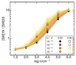
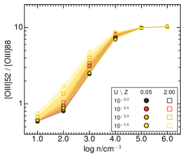
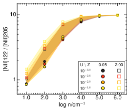
Figure 10: Same as Figure 1 but for the $\alpha_{\rm AGN}=-1.4$ AGN models.

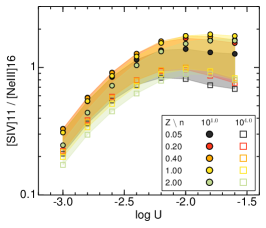
Figure 11: Same as Figure 2 but for the $\alpha_{\rm AGN}=-1.4$ AGN models.

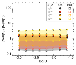
Figure 12: Same as Figure 3 but for the $\alpha_{\rm AGN}=-1.4$ AGN models.

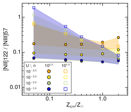
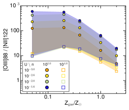
Figure 13: Same as Figure 4 but for the $\alpha_{\rm AGN}=-1.4$ AGN models.

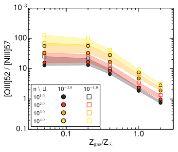
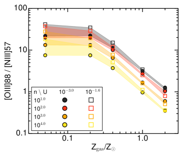
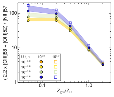
Figure 14: Same as Figure LABEL:fig:o3_n3 but for the $\alpha_{\rm AGN}=-1.4$ AGN models.

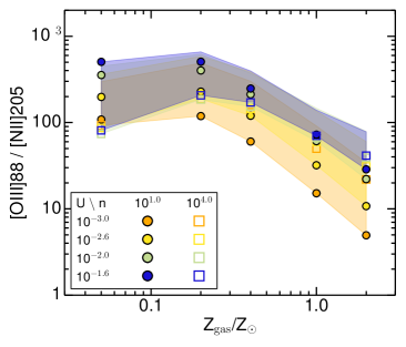
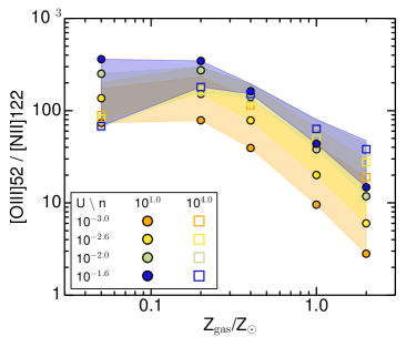
Figure 15: Same as Figure LABEL:fig:Z_o3 but for the $\alpha_{\rm AGN}=-1.4$ AGN models.

Table 4: Logarithm of the mid- and far-IR line ratios for the AGN models

$Z/Z_{\odot}$	$\log\frac{n_{\rm H}}{{\rm cm^{-3}}}$	$\log\,U$	$\frac{{\rm[S\,{\scriptscriptstyle III}]19}}{{\rm[S\,{\scriptscriptstyle III}]33}}$	$\frac{{\rm[O\,{\scriptscriptstyle III}]52}}{{\rm[O\,{\scriptscriptstyle III}]88}}$	$\frac{{\rm[N\,{\scriptscriptstyle II}]122}}{{\rm[N\,{\scriptscriptstyle II}]205}}$	$\frac{{\rm[S\,{\scriptscriptstyle IV}]11}}{{\rm[Ne\,{\scriptscriptstyle III}]16}}$	$\frac{{\rm[Ne\,{\scriptscriptstyle II}]13}}{{\rm[Ne\,{\scriptscriptstyle III}]16}}$	$\frac{{\rm[O\,{\scriptscriptstyle III}]52}}{{\rm[N\,{\scriptscriptstyle III}]57}}$	$\frac{{\rm[O\,{\scriptscriptstyle III}]88}}{{\rm[N\,{\scriptscriptstyle III}]57}}$	$\frac{{\rm[O\,{\scriptscriptstyle III}]52}}{{\rm[N\,{\scriptscriptstyle II}]122}}$	$\frac{{\rm[O\,{\scriptscriptstyle III}]52}}{{\rm[N\,{\scriptscriptstyle II}]205}}$	$\frac{{\rm[O\,{\scriptscriptstyle III}]88}}{{\rm[N\,{\scriptscriptstyle II}]122}}$	$\frac{{\rm[O\,{\scriptscriptstyle III}]88}}{{\rm[N\,{\scriptscriptstyle II}]205}}$
0.05	1	–3.0	–0.37	–0.23	–0.06	–0.51	0.18	1.11	1.34	1.87	1.81	2.09	2.04
0.05	1	–2.8	–0.37	–0.23	–0.06	–0.27	0.18	1.11	1.34	2.02	1.96	2.24	2.18
0.05	1	–2.6	–0.37	–0.23	–0.06	–0.07	0.18	1.11	1.34	2.13	2.07	2.36	2.30
0.05	1	–2.4	–0.37	–0.22	–0.07	0.06	0.18	1.13	1.36	2.23	2.17	2.46	2.39
0.05	1	–2.2	–0.37	–0.22	–0.07	0.13	0.17	1.17	1.39	2.32	2.25	2.54	2.47
0.05	1	–2.0	–0.37	–0.22	–0.07	0.14	0.15	1.23	1.45	2.40	2.33	2.62	2.55
0.05	1	–1.8	–0.37	–0.22	–0.07	0.12	0.11	1.31	1.53	2.48	2.41	2.70	2.63
0.05	1	–1.6	–0.37	–0.21	–0.07	0.11	0.07	1.40	1.62	2.56	2.49	2.77	2.70
0.05	2	–3.0	–0.34	–0.10	0.28	–0.51	0.21	1.20	1.30	1.99	2.27	2.08	2.36
0.05	2	–2.8	–0.34	–0.09	0.26	–0.27	0.21	1.20	1.29	2.13	2.39	2.22	2.48
0.05	2	–2.6	–0.33	–0.09	0.24	–0.08	0.21	1.21	1.30	2.23	2.47	2.32	2.56
0.05	2	–2.4	–0.33	–0.09	0.22	0.06	0.21	1.23	1.31	2.30	2.52	2.39	2.61
0.05	2	–2.2	–0.33	–0.08	0.21	0.13	0.20	1.27	1.35	2.35	2.55	2.43	2.64
0.05	2	–2.0	–0.33	–0.08	0.20	0.14	0.18	1.33	1.41	2.38	2.58	2.45	2.65
0.05	2	–1.8	–0.33	–0.07	0.20	0.11	0.15	1.42	1.48	2.40	2.59	2.46	2.66
0.05	2	–1.6	–0.33	–0.05	0.20	0.09	0.12	1.52	1.57	2.40	2.60	2.45	2.65
0.05	3	–3.0	–0.16	0.39	0.63	–0.52	0.28	1.51	1.12	2.24	2.87	1.85	2.47
0.05	3	–2.8	–0.15	0.39	0.62	–0.28	0.28	1.51	1.12	2.29	2.91	1.90	2.52
0.05	3	–2.6	–0.14	0.39	0.62	–0.10	0.29	1.52	1.13	2.30	2.92	1.91	2.53
0.05	3	–2.4	–0.13	0.39	0.62	0.03	0.29	1.54	1.15	2.28	2.90	1.89	2.50
0.05	3	–2.2	–0.13	0.39	0.62	0.10	0.29	1.58	1.19	2.24	2.86	1.84	2.47
0.05	3	–2.0	–0.13	0.39	0.63	0.10	0.28	1.64	1.25	2.19	2.82	1.80	2.43
0.05	3	–1.8	–0.12	0.39	0.65	0.07	0.26	1.74	1.34	2.15	2.79	1.75	2.40
0.05	3	–1.6	–0.11	0.40	0.66	0.05	0.23	1.85	1.44	2.12	2.78	1.71	2.38
0.05	4	–3.0	0.21	0.87	0.89	–0.68	0.51	1.75	0.88	1.95	2.84	1.08	1.97
0.05	4	–2.8	0.24	0.87	0.89	–0.44	0.53	1.75	0.87	1.95	2.84	1.07	1.97
0.05	4	–2.6	0.26	0.87	0.89	–0.26	0.55	1.75	0.88	1.91	2.81	1.04	1.94
0.05	4	–2.4	0.27	0.87	0.90	–0.14	0.57	1.78	0.91	1.88	2.77	1.01	1.91
0.05	4	–2.2	0.29	0.87	0.90	–0.08	0.58	1.82	0.95	1.84	2.74	0.98	1.88
0.05	4	–2.0	0.30	0.86	0.91	–0.09	0.59	1.89	1.03	1.82	2.73	0.96	1.87
0.05	4	–1.8	0.31	0.85	0.91	–0.14	0.59	1.99	1.14	1.82	2.73	0.97	1.88
0.05	4	–1.6	0.33	0.84	0.92	–0.17	0.60	2.11	1.26	1.83	2.75	0.99	1.91
0.05	5	–3.0	0.67	1.00	0.97	–1.19	1.00	1.79	0.79	1.47	2.45	0.47	1.45
0.05	5	–2.8	0.70	1.00	0.98	–0.96	0.99	1.79	0.79	1.48	2.46	0.49	1.46
0.05	5	–2.6	0.72	1.00	0.98	–0.78	0.98	1.80	0.80	1.48	2.46	0.48	1.46
0.05	5	–2.4	0.73	1.00	0.98	–0.66	0.99	1.82	0.82	1.48	2.45	0.48	1.46
0.05	5	–2.2	0.74	1.00	0.98	–0.60	0.99	1.87	0.87	1.48	2.46	0.48	1.46
0.05	5	–2.0	0.75	1.00	0.98	–0.61	0.99	1.95	0.95	1.50	2.48	0.50	1.48
0.05	5	–1.8	0.76	1.00	0.98	–0.66	0.98	2.05	1.05	1.54	2.52	0.54	1.52
0.05	5	–1.6	0.77	0.99	0.98	–0.70	0.97	2.17	1.18	1.58	2.57	0.59	1.57
0.05	6	–3.0	0.96	1.01	0.99	–1.82	1.38	1.80	0.78	1.19	2.18	0.17	1.16
0.05	6	–2.8	0.97	1.01	0.99	–1.60	1.35	1.80	0.78	1.20	2.19	0.19	1.18
0.05	6	–2.6	0.97	1.01	0.99	–1.43	1.33	1.80	0.79	1.20	2.19	0.19	1.18
0.05	6	–2.4	0.97	1.01	0.99	–1.31	1.30	1.83	0.81	1.20	2.19	0.18	1.17
0.05	6	–2.2	0.97	1.01	0.99	–1.24	1.26	1.87	0.86	1.20	2.19	0.18	1.17
0.05	6	–2.0	0.98	1.02	0.99	–1.23	1.22	1.95	0.93	1.22	2.21	0.20	1.19
0.05	6	–1.8	0.98	1.02	0.99	–1.25	1.17	2.05	1.03	1.26	2.25	0.24	1.23
0.05	6	–1.6	0.99	1.02	0.99	–1.25	1.12	2.16	1.14	1.31	2.30	0.29	1.28
0.20	1	–3.0	–0.37	–0.23	–0.05	–0.48	–0.21	1.12	1.35	1.90	1.85	2.12	2.07
0.20	1	–2.8	–0.36	–0.23	–0.05	–0.24	–0.22	1.12	1.34	2.05	2.01	2.28	2.23
0.20	1	–2.6	–0.36	–0.22	–0.05	–0.04	–0.22	1.12	1.34	2.18	2.13	2.41	2.36
0.20	1	–2.4	–0.36	–0.22	–0.05	0.11	–0.21	1.14	1.36	2.28	2.23	2.51	2.46
0.20	1	–2.2	–0.36	–0.22	–0.05	0.20	–0.21	1.17	1.39	2.37	2.32	2.59	2.54
0.20	1	–2.0	–0.36	–0.22	–0.05	0.23	–0.22	1.21	1.43	2.44	2.39	2.65	2.60
0.20	1	–1.8	–0.36	–0.21	–0.05	0.22	–0.23	1.27	1.48	2.50	2.45	2.71	2.66
0.20	1	–1.6	–0.37	–0.20	–0.04	0.19	–0.25	1.33	1.54	2.54	2.50	2.74	2.70
0.20	2	–3.0	–0.33	–0.09	0.34	–0.48	–0.16	1.21	1.30	2.03	2.37	2.12	2.46
0.20	2	–2.8	–0.32	–0.09	0.33	–0.24	–0.17	1.21	1.30	2.18	2.51	2.26	2.59
0.20	2	–2.6	–0.32	–0.08	0.31	–0.04	–0.16	1.22	1.30	2.29	2.60	2.37	2.68
0.20	2	–2.4	–0.32	–0.07	0.29	0.10	–0.16	1.24	1.31	2.38	2.67	2.45	2.74
0.20	2	–2.2	–0.32	–0.06	0.28	0.19	–0.15	1.27	1.33	2.43	2.71	2.49	2.77
0.20	2	–2.0	–0.31	–0.04	0.28	0.22	–0.16	1.32	1.37	2.47	2.75	2.51	2.79
0.20	2	–1.8	–0.31	–0.02	0.29	0.21	–0.17	1.39	1.41	2.50	2.79	2.52	2.81
0.20	2	–1.6	–0.30	0.01	0.31	0.18	–0.18	1.47	1.46	2.52	2.83	2.51	2.82
0.20	3	–3.0	–0.10	0.40	0.72	–0.50	–0.07	1.52	1.12	2.37	3.09	1.96	2.69
0.20	3	–2.8	–0.09	0.41	0.71	–0.26	–0.07	1.52	1.11	2.45	3.16	2.04	2.75
0.20	3	–2.6	–0.09	0.41	0.71	–0.06	–0.05	1.53	1.11	2.48	3.18	2.06	2.77
0.20	3	–2.4	–0.08	0.42	0.71	0.08	–0.03	1.55	1.12	2.47	3.18	2.05	2.76
0.20	3	–2.2	–0.07	0.43	0.71	0.16	–0.02	1.58	1.15	2.46	3.17	2.02	2.73
0.20	3	–2.0	–0.06	0.45	0.73	0.18	–0.00	1.64	1.19	2.44	3.16	1.99	2.71
0.20	3	–1.8	–0.05	0.47	0.74	0.16	0.01	1.71	1.23	2.43	3.17	1.95	2.70
0.20	3	–1.6	–0.02	0.50	0.77	0.12	0.02	1.79	1.29	2.42	3.19	1.92	2.69
0.20	4	–3.0	0.30	0.88	0.93	–0.65	0.25	1.75	0.87	2.22	3.15	1.34	2.27
0.20	4	–2.8	0.32	0.88	0.93	–0.41	0.28	1.75	0.87	2.23	3.16	1.35	2.28
0.20	4	–2.6	0.34	0.88	0.93	–0.23	0.32	1.76	0.88	2.22	3.15	1.34	2.27
0.20	4	–2.4	0.36	0.88	0.93	–0.10	0.35	1.77	0.89	2.21	3.14	1.33	2.26
0.20	4	–2.2	0.39	0.88	0.94	–0.03	0.37	1.81	0.92	2.20	3.14	1.32	2.26
0.20	4	–2.0	0.41	0.89	0.94	–0.02	0.37	1.86	0.97	2.21	3.15	1.32	2.27
0.20	4	–1.8	0.44	0.89	0.95	–0.06	0.51	1.92	1.03	2.23	3.18	1.33	2.28
0.20	4	–1.6	0.49	0.90	0.96	–0.12	0.54	1.99	1.10	2.26	3.21	1.36	2.32
0.20	5	–3.0	0.75	1.00	0.98	–1.14	0.74	1.79	0.80	1.85	2.84	0.86	1.84
0.20	5	–2.8	0.77	1.00	0.98	–0.90	0.74	1.79	0.79	1.89	2.87	0.89	1.87
0.20	5	–2.6	0.80	1.00	0.98	–0.71	0.73	1.80	0.80	1.91	2.90	0.91	1.90
0.20	5	–2.4	0.82	1.00	0.99	–0.59	0.78	1.82	0.82	1.94	2.92	0.94	1.92
0.20	5	–2.2	0.84	1.00	0.99	–0.52	0.78	1.85	0.85	1.97	2.96	0.97	1.96
0.20	5	–2.0	0.82	1.00	0.99	–0.56	1.12	1.90	0.90	2.01	3.00	1.01	2.00
0.20	5	–1.8	0.82	1.00	0.99	–0.60	1.05	1.97	0.97	2.06	3.05	1.06	2.05
0.20	5	–1.6	0.84	1.00	0.99	–0.67	1.00	2.04	1.04	2.13	3.11	1.12	2.11
0.20	6	–3.0	0.98	1.01	0.99	–1.71	1.34	1.80	0.79	1.66	2.65	0.64	1.63
0.20	6	–2.8	0.99	1.01	0.99	–1.47	1.29	1.80	0.78	1.71	2.70	0.70	1.69
0.20	6	–2.6	0.99	1.01	0.99	–1.30	1.25	1.80	0.79	1.76	2.75	0.74	1.73
0.20	6	–2.4	0.99	1.01	0.99	–1.17	1.20	1.82	0.81	1.80	2.80	0.79	1.78
0.20	6	–2.2	0.99	1.01	0.99	–1.09	1.15	1.86	0.85	1.86	2.86	0.85	1.84
0.20	6	–2.0	1.00	1.01	0.99	–1.07	1.09	1.91	0.90	1.93	2.92	0.92	1.91
0.20	6	–1.8	1.00	1.02	0.99	–1.09	1.03	1.98	0.96	2.01	3.00	0.99	1.99
0.20	6	–1.6	1.01	1.02	0.99	–1.13	0.98	2.05	1.03	2.08	3.08	1.07	2.06
0.40	1	–3.0	–0.37	–0.23	–0.04	–0.48	–0.42	0.82	1.05	1.60	1.55	1.82	1.78
0.40	1	–2.8	–0.36	–0.23	–0.04	–0.24	–0.44	0.82	1.05	1.76	1.72	1.99	1.95
0.40	1	–2.6	–0.36	–0.22	–0.04	–0.04	–0.44	0.82	1.05	1.89	1.86	2.12	2.08
0.40	1	–2.4	–0.36	–0.22	–0.04	0.11	–0.43	0.84	1.06	2.00	1.96	2.22	2.18
0.40	1	–2.2	–0.36	–0.22	–0.04	0.21	–0.42	0.86	1.08	2.09	2.05	2.30	2.27
0.40	1	–2.0	–0.36	–0.21	–0.03	0.25	–0.41	0.90	1.11	2.15	2.12	2.36	2.33
0.40	1	–1.8	–0.36	–0.20	–0.03	0.24	–0.40	0.94	1.14	2.19	2.17	2.39	2.37
0.40	1	–1.6	–0.36	–0.20	–0.01	0.22	–0.40	0.98	1.18	2.21	2.20	2.41	2.39
0.40	2	–3.0	–0.32	–0.08	0.37	–0.49	–0.36	0.92	1.00	1.74	2.11	1.82	2.19
0.40	2	–2.8	–0.31	–0.07	0.36	–0.24	–0.37	0.92	0.99	1.90	2.26	1.97	2.33
0.40	2	–2.6	–0.31	–0.06	0.35	–0.05	–0.36	0.93	0.99	2.02	2.38	2.09	2.44
0.40	2	–2.4	–0.31	–0.05	0.34	0.10	–0.35	0.94	0.99	2.12	2.46	2.17	2.51
0.40	2	–2.2	–0.31	–0.03	0.33	0.20	–0.34	0.97	1.01	2.19	2.52	2.22	2.55
0.40	2	–2.0	–0.30	–0.01	0.33	0.24	–0.33	1.02	1.03	2.23	2.56	2.24	2.57
0.40	2	–1.8	–0.30	0.02	0.35	0.23	–0.32	1.07	1.05	2.26	2.61	2.24	2.59
0.40	2	–1.6	–0.29	0.06	0.38	0.20	–0.31	1.13	1.08	2.27	2.65	2.22	2.60
0.40	3	–3.0	–0.06	0.42	0.77	–0.50	–0.25	1.23	0.81	2.13	2.90	1.71	2.48
0.40	3	–2.8	–0.06	0.43	0.76	–0.26	–0.24	1.23	0.80	2.23	2.98	1.80	2.56
0.40	3	–2.6	–0.05	0.44	0.75	–0.07	–0.22	1.24	0.80	2.28	3.03	1.84	2.59
0.40	3	–2.4	–0.04	0.45	0.75	0.08	–0.19	1.25	0.80	2.29	3.04	1.84	2.59
0.40	3	–2.2	–0.03	0.47	0.75	0.17	–0.15	1.28	0.81	2.29	3.05	1.83	2.58
0.40	3	–2.0	–0.02	0.49	0.77	0.20	–0.12	1.32	0.83	2.29	3.06	1.80	2.57
0.40	3	–1.8	0.00	0.52	0.79	0.19	–0.08	1.38	0.86	2.29	3.08	1.77	2.56
0.40	3	–1.6	0.04	0.55	0.82	0.15	–0.02	1.44	0.89	2.29	3.11	1.74	2.56
0.40	4	–3.0	0.35	0.88	0.94	–0.66	0.11	1.45	0.57	2.06	3.00	1.18	2.12
0.40	4	–2.8	0.37	0.88	0.94	–0.42	0.14	1.45	0.56	2.09	3.04	1.21	2.15
0.40	4	–2.6	0.40	0.89	0.94	–0.24	0.15	1.45	0.56	2.10	3.05	1.21	2.16
0.40	4	–2.4	0.42	0.89	0.95	–0.10	0.21	1.46	0.57	2.10	3.05	1.21	2.16
0.40	4	–2.2	0.45	0.89	0.95	–0.02	0.25	1.49	0.59	2.11	3.06	1.22	2.17
0.40	4	–2.0	0.48	0.90	0.96	–0.00	0.28	1.53	0.63	2.13	3.08	1.23	2.19
0.40	4	–1.8	0.52	0.91	0.96	–0.03	0.32	1.57	0.67	2.16	3.12	1.25	2.21
0.40	4	–1.6	0.56	0.91	0.97	–0.10	0.36	1.62	0.71	2.18	3.15	1.27	2.23
0.40	5	–3.0	0.78	1.00	0.99	–1.13	0.58	1.49	0.49	1.77	2.75	0.77	1.75
0.40	5	–2.8	0.81	1.00	0.99	–0.89	0.57	1.49	0.49	1.81	2.80	0.82	1.80
0.40	5	–2.6	0.84	1.00	0.99	–0.70	0.56	1.49	0.49	1.85	2.84	0.85	1.84
0.40	5	–2.4	0.86	1.00	0.99	–0.56	0.56	1.50	0.50	1.89	2.88	0.89	1.88
0.40	5	–2.2	0.88	1.00	0.99	–0.48	0.57	1.53	0.53	1.94	2.93	0.94	1.93
0.40	5	–2.0	0.87	1.00	0.99	–0.50	0.88	1.57	0.57	1.99	2.98	0.99	1.98
0.40	5	–1.8	0.88	1.00	0.99	–0.54	0.85	1.62	0.62	2.05	3.04	1.05	2.04
0.40	5	–1.6	0.89	1.00	0.99	–0.62	0.82	1.67	0.66	2.10	3.09	1.10	2.09
0.40	6	–3.0	1.00	1.01	0.99	–1.60	1.12	1.49	0.48	1.63	2.62	0.62	1.61
0.40	6	–2.8	1.01	1.01	0.99	–1.36	1.10	1.49	0.48	1.70	2.70	0.69	1.68
0.40	6	–2.6	1.01	1.01	0.99	–1.18	1.06	1.50	0.48	1.77	2.76	0.75	1.75
0.40	6	–2.4	1.01	1.01	0.99	–1.04	1.03	1.51	0.50	1.83	2.82	0.82	1.81
0.40	6	–2.2	1.01	1.01	0.99	–0.97	0.98	1.54	0.53	1.90	2.90	0.89	1.88
0.40	6	–2.0	1.01	1.01	0.99	–0.95	0.94	1.59	0.57	1.98	2.97	0.96	1.95
0.40	6	–1.8	1.02	1.01	0.99	–0.97	0.89	1.64	0.62	2.05	3.04	1.03	2.03
0.40	6	–1.6	1.02	1.01	0.99	–1.03	0.85	1.68	0.67	2.11	3.10	1.09	2.09
1.00	1	–3.0	–0.38	–0.23	–0.03	–0.51	–0.67	0.27	0.50	0.98	0.95	1.21	1.18
1.00	1	–2.8	–0.38	–0.23	–0.02	–0.26	–0.71	0.26	0.49	1.16	1.13	1.38	1.36
1.00	1	–2.6	–0.37	–0.22	–0.02	–0.07	–0.72	0.26	0.48	1.30	1.28	1.52	1.51
1.00	1	–2.4	–0.37	–0.21	–0.01	0.09	–0.71	0.27	0.48	1.42	1.41	1.63	1.62
1.00	1	–2.2	–0.37	–0.21	–0.00	0.19	–0.69	0.29	0.49	1.51	1.51	1.72	1.71
1.00	1	–2.0	–0.37	–0.20	0.01	0.25	–0.67	0.31	0.51	1.58	1.59	1.78	1.78
1.00	1	–1.8	–0.37	–0.18	0.02	0.26	–0.65	0.34	0.52	1.62	1.65	1.81	1.83
1.00	1	–1.6	–0.37	–0.17	0.05	0.25	–0.62	0.37	0.54	1.64	1.69	1.81	1.86
1.00	2	–3.0	–0.31	–0.06	0.41	–0.51	–0.59	0.38	0.43	1.15	1.56	1.20	1.62
1.00	2	–2.8	–0.31	–0.04	0.41	–0.27	–0.61	0.37	0.42	1.32	1.74	1.37	1.78
1.00	2	–2.6	–0.30	–0.02	0.41	–0.07	–0.61	0.38	0.41	1.47	1.88	1.49	1.90
1.00	2	–2.4	–0.30	–0.00	0.41	0.08	–0.59	0.40	0.40	1.58	1.99	1.58	1.99
1.00	2	–2.2	–0.29	0.03	0.41	0.19	–0.57	0.42	0.39	1.67	2.08	1.64	2.05
1.00	2	–2.0	–0.28	0.06	0.42	0.24	–0.55	0.46	0.39	1.73	2.15	1.67	2.09
1.00	2	–1.8	–0.27	0.10	0.44	0.25	–0.53	0.50	0.40	1.78	2.22	1.68	2.12
1.00	2	–1.6	–0.25	0.14	0.48	0.24	–0.49	0.54	0.40	1.80	2.28	1.66	2.14
1.00	3	–3.0	–0.00	0.46	0.82	–0.53	–0.45	0.68	0.22	1.60	2.42	1.14	1.96
1.00	3	–2.8	0.00	0.47	0.81	–0.28	–0.44	0.68	0.21	1.73	2.54	1.26	2.07
1.00	3	–2.6	0.01	0.49	0.80	–0.09	–0.41	0.68	0.19	1.81	2.62	1.33	2.13
1.00	3	–2.4	0.03	0.51	0.80	0.06	–0.38	0.69	0.19	1.86	2.67	1.36	2.16
1.00	3	–2.2	0.04	0.53	0.81	0.16	–0.35	0.71	0.19	1.89	2.69	1.36	2.17
1.00	3	–2.0	0.07	0.55	0.82	0.20	–0.32	0.74	0.19	1.90	2.72	1.35	2.17
1.00	3	–1.8	0.10	0.58	0.83	0.21	–0.29	0.78	0.20	1.91	2.74	1.33	2.16
1.00	3	–1.6	0.14	0.62	0.86	0.18	–0.24	0.82	0.21	1.91	2.76	1.29	2.14
1.00	4	–3.0	0.43	0.89	0.96	–0.70	–0.07	0.88	–0.02	1.63	2.59	0.74	1.70
1.00	4	–2.8	0.45	0.90	0.96	–0.47	–0.06	0.87	–0.02	1.69	2.65	0.79	1.75
1.00	4	–2.6	0.48	0.90	0.96	–0.29	–0.04	0.87	–0.03	1.72	2.68	0.82	1.78
1.00	4	–2.4	0.50	0.91	0.96	–0.15	–0.02	0.88	–0.03	1.73	2.69	0.83	1.79
1.00	4	–2.2	0.53	0.91	0.96	–0.05	–0.00	0.89	–0.02	1.75	2.71	0.84	1.80
1.00	4	–2.0	0.57	0.91	0.96	–0.01	0.02	0.91	0.00	1.77	2.74	0.86	1.82
1.00	4	–1.8	0.60	0.92	0.97	–0.03	0.06	0.94	0.02	1.79	2.76	0.87	1.84
1.00	4	–1.6	0.65	0.93	0.97	–0.08	0.11	0.98	0.05	1.80	2.78	0.87	1.85
1.00	5	–3.0	0.83	1.00	0.99	–1.16	0.37	0.91	–0.09	1.41	2.40	0.41	1.40
1.00	5	–2.8	0.85	1.00	0.99	–0.93	0.35	0.91	–0.09	1.47	2.46	0.47	1.46
1.00	5	–2.6	0.87	1.00	0.99	–0.74	0.34	0.91	–0.09	1.51	2.50	0.51	1.50
1.00	5	–2.4	0.90	1.00	0.99	–0.59	0.34	0.91	–0.09	1.56	2.55	0.56	1.55
1.00	5	–2.2	0.91	1.00	0.99	–0.49	0.35	0.93	–0.07	1.61	2.59	0.60	1.59
1.00	5	–2.0	0.93	1.00	0.99	–0.46	0.38	0.95	–0.05	1.66	2.65	0.65	1.64
1.00	5	–1.8	0.95	1.00	0.99	–0.48	0.41	0.99	–0.02	1.70	2.70	0.70	1.69
1.00	5	–1.6	0.94	1.00	0.99	–0.56	0.63	1.02	0.01	1.74	2.73	0.73	1.72
1.00	6	–3.0	1.01	1.01	0.99	–1.53	0.88	0.91	–0.10	1.31	2.30	0.30	1.29
1.00	6	–2.8	1.02	1.01	0.99	–1.28	0.86	0.91	–0.10	1.39	2.38	0.38	1.37
1.00	6	–2.6	1.02	1.01	0.99	–1.09	0.85	0.91	–0.10	1.46	2.45	0.45	1.44
1.00	6	–2.4	1.03	1.01	0.99	–0.94	0.82	0.92	–0.09	1.53	2.52	0.51	1.51
1.00	6	–2.2	1.03	1.01	0.99	–0.85	0.80	0.94	–0.07	1.60	2.59	0.58	1.58
1.00	6	–2.0	1.03	1.01	0.99	–0.82	0.77	0.97	–0.04	1.66	2.66	0.65	1.64
1.00	6	–1.8	1.03	1.01	0.99	–0.83	0.74	1.01	–0.01	1.72	2.72	0.71	1.70
1.00	6	–1.6	1.03	1.01	0.99	–0.88	0.72	1.04	0.03	1.77	2.76	0.76	1.75
2.00	1	–3.0	–0.41	–0.23	0.01	–0.61	–0.74	–0.13	0.10	0.45	0.46	0.68	0.69
2.00	1	–2.8	–0.41	–0.22	0.02	–0.35	–0.78	–0.14	0.08	0.63	0.65	0.85	0.88
2.00	1	–2.6	–0.40	–0.22	0.04	–0.14	–0.80	–0.15	0.07	0.78	0.82	0.99	1.03
2.00	1	–2.4	–0.40	–0.20	0.05	0.02	–0.80	–0.14	0.06	0.90	0.95	1.11	1.16
2.00	1	–2.2	–0.40	–0.19	0.07	0.12	–0.79	–0.13	0.06	1.00	1.07	1.19	1.26
2.00	1	–2.0	–0.39	–0.17	0.10	0.19	–0.76	–0.12	0.06	1.07	1.17	1.24	1.34
2.00	1	–1.8	–0.39	–0.15	0.13	0.21	–0.74	–0.10	0.06	1.13	1.26	1.28	1.41
2.00	1	–1.6	–0.38	–0.12	0.16	0.21	–0.71	–0.07	0.05	1.17	1.33	1.29	1.46
2.00	2	–3.0	–0.32	–0.03	0.47	–0.59	–0.63	–0.01	0.01	0.67	1.15	0.70	1.17
2.00	2	–2.8	–0.31	–0.01	0.48	–0.33	–0.65	–0.02	–0.01	0.86	1.34	0.87	1.35
2.00	2	–2.6	–0.30	0.02	0.48	–0.12	–0.66	–0.01	–0.03	1.02	1.50	1.00	1.48
2.00	2	–2.4	–0.29	0.05	0.49	0.03	–0.66	0.00	–0.05	1.16	1.64	1.10	1.59
2.00	2	–2.2	–0.27	0.09	0.50	0.14	–0.64	0.03	–0.07	1.26	1.76	1.17	1.67
2.00	2	–2.0	–0.25	0.14	0.52	0.20	–0.63	0.06	–0.08	1.35	1.87	1.22	1.74
2.00	2	–1.8	–0.23	0.18	0.55	0.22	–0.61	0.09	–0.09	1.42	1.97	1.24	1.79
2.00	2	–1.6	–0.19	0.23	0.59	0.22	–0.58	0.13	–0.10	1.47	2.06	1.24	1.83
2.00	3	–3.0	0.06	0.50	0.86	–0.58	–0.49	0.28	–0.22	1.18	2.04	0.68	1.54
2.00	3	–2.8	0.06	0.52	0.85	–0.33	–0.49	0.27	–0.24	1.35	2.20	0.83	1.68
2.00	3	–2.6	0.08	0.53	0.85	–0.13	–0.48	0.27	–0.26	1.46	2.31	0.93	1.78
2.00	3	–2.4	0.10	0.55	0.85	0.02	–0.47	0.28	–0.27	1.55	2.39	0.99	1.84
2.00	3	–2.2	0.12	0.58	0.85	0.12	–0.46	0.30	–0.28	1.61	2.45	1.03	1.88
2.00	3	–2.0	0.16	0.60	0.86	0.17	–0.44	0.32	–0.29	1.64	2.50	1.04	1.90
2.00	3	–1.8	0.20	0.63	0.87	0.19	–0.42	0.34	–0.29	1.67	2.54	1.03	1.90
2.00	3	–1.6	0.25	0.67	0.89	0.17	–0.38	0.38	–0.29	1.67	2.56	1.00	1.89
2.00	4	–3.0	0.49	0.91	0.97	–0.76	–0.15	0.45	–0.45	1.28	2.25	0.37	1.34
2.00	4	–2.8	0.51	0.91	0.97	–0.53	–0.16	0.44	–0.47	1.38	2.34	0.47	1.44
2.00	4	–2.6	0.54	0.91	0.97	–0.34	–0.16	0.44	–0.47	1.44	2.41	0.53	1.49
2.00	4	–2.4	0.58	0.92	0.97	–0.20	–0.16	0.44	–0.48	1.48	2.45	0.56	1.53
2.00	4	–2.2	0.61	0.92	0.97	–0.10	–0.16	0.45	–0.48	1.52	2.49	0.60	1.56
2.00	4	–2.0	0.64	0.93	0.97	–0.05	–0.14	0.46	–0.47	1.55	2.52	0.62	1.59
2.00	4	–1.8	0.68	0.93	0.97	–0.05	–0.11	0.48	–0.45	1.57	2.54	0.64	1.61
2.00	4	–1.6	0.72	0.94	0.97	–0.10	–0.06	0.50	–0.44	1.58	2.56	0.64	1.62
2.00	5	–3.0	0.85	1.00	0.99	–1.21	0.24	0.48	–0.52	1.12	2.11	0.12	1.11
2.00	5	–2.8	0.88	1.00	0.99	–0.97	0.22	0.47	–0.53	1.20	2.19	0.20	1.19
2.00	5	–2.6	0.90	1.00	0.99	–0.78	0.21	0.47	–0.53	1.27	2.26	0.27	1.26
2.00	5	–2.4	0.92	1.00	0.99	–0.63	0.21	0.47	–0.53	1.33	2.31	0.33	1.31
2.00	5	–2.2	0.94	1.00	0.99	–0.52	0.22	0.48	–0.52	1.38	2.37	0.38	1.37
2.00	5	–2.0	0.95	1.00	0.99	–0.46	0.24	0.49	–0.51	1.43	2.42	0.43	1.42
2.00	5	–1.8	0.97	1.00	0.99	–0.46	0.29	0.51	–0.49	1.48	2.47	0.48	1.47
2.00	5	–1.6	0.97	1.00	0.99	–0.51	0.45	0.53	–0.47	1.50	2.49	0.50	1.49
2.00	6	–3.0	1.02	1.01	0.99	–1.49	0.67	0.47	–0.54	1.04	2.04	0.03	1.02
2.00	6	–2.8	1.02	1.01	0.99	–1.24	0.65	0.47	–0.54	1.14	2.13	0.13	1.12
2.00	6	–2.6	1.03	1.01	0.99	–1.04	0.64	0.47	–0.54	1.22	2.21	0.21	1.20
2.00	6	–2.4	1.03	1.01	0.99	–0.89	0.65	0.48	–0.54	1.29	2.29	0.28	1.27
2.00	6	–2.2	1.03	1.01	0.99	–0.79	0.64	0.49	–0.52	1.37	2.36	0.35	1.35
2.00	6	–2.0	1.03	1.01	0.99	–0.74	0.62	0.51	–0.50	1.43	2.42	0.42	1.41
2.00	6	–1.8	1.04	1.01	0.99	–0.74	0.61	0.53	–0.48	1.49	2.48	0.48	1.47
2.00	6	–1.6	1.04	1.01	0.99	–0.77	0.61	0.55	–0.46	1.53	2.52	0.52	1.51

References

- Abel et al. (2009) Abel N. P., Dudley C., Fischer J., Satyapal S., van Hoof P. A. M., 2009, ApJ, 701, 1147
- Ádámkovics et al. (2011) Ádámkovics M., Glassgold A. E., Meijerink R., 2011, ApJ, 736, 143
- Alloin et al. (1979) Alloin D., Collin-Souffrin S., Joly M., Vigroux L., 1979, A&A, 78, 200
- Asplund et al. (2009) Asplund M., Grevesse N., Sauval A. J., Scott P., 2009, ARA&A, 47, 481
- Berg et al. (2016) Berg D. A., Skillman E. D., Henry R. B. C., Erb D. K., Carigi L., 2016, ApJ, 827, 126
- Béthermin et al. (2016) Béthermin M., et al., 2016, A&A, 586, L7
- Braito et al. (2009) Braito V., Reeves J. N., Della Ceca R., Ptak A., Risaliti G., Yaqoob T., 2009, A&A, 504, 53
- Brooks et al. (2007) Brooks A. M., Governato F., Booth C. M., Willman B., Gardner J. P., Wadsley J., Stinson G., Quinn T., 2007, ApJ, 655, L17
- Caputi et al. (2008) Caputi K. I., et al., 2008, ApJ, 680, 939
- Casey et al. (2014) Casey C. M., Narayanan D., Cooray A., 2014, Phys. Rep., 541, 45
- Cazaux & Tielens (2004) Cazaux S., Tielens A. G. G. M., 2004, ApJ, 604, 222
- Dasyra et al. (2006a) Dasyra K. M., et al., 2006a, ApJ, 638, 745
- Dasyra et al. (2006b) Dasyra K. M., et al., 2006b, ApJ, 651, 835
- De Looze et al. (2014) De Looze I., et al., 2014, A&A, 568, A62
- Dopita et al. (2006) Dopita M. A., et al., 2006, ApJS, 167, 177
- Draine (2011) Draine B. T., 2011, Physics of the Interstellar and Intergalactic Medium
- Edmunds & Pagel (1984) Edmunds M. G., Pagel B. E. J., 1984, MNRAS, 211, 507
- Efstathiou et al. (2014) Efstathiou A., et al., 2014, MNRAS, 437, L16
- Farrah et al. (2007) Farrah D., et al., 2007, ApJ, 667, 149
- Farrah et al. (2013) Farrah D., et al., 2013, ApJ, 776, 38
- Feigelson & Nelson (1985) Feigelson E. D., Nelson P. I., 1985, ApJ, 293, 192
- Ferland et al. (2013) Ferland G. J., et al., 2013, Rev. Mex. Astron. Astrofis., 49, 137
- Fernández-Ontiveros et al. (2016) Fernández-Ontiveros J. A., Spinoglio L., Pereira-Santaella M., Malkan M. A., Andreani P., Dasyra K. M., 2016, ApJS, 226, 19
- Finlator & Davé (2008) Finlator K., Davé R., 2008, MNRAS, 385, 2181
- Garnett et al. (1999) Garnett D. R., Shields G. A., Peimbert M., Torres-Peimbert S., Skillman E. D., Dufour R. J., Terlevich E., Terlevich R. J., 1999, ApJ, 513, 168
- Genzel et al. (2001) Genzel R., Tacconi L. J., Rigopoulou D., Lutz D., Tecza M., 2001, ApJ, 563, 527
- Glassgold et al. (2007) Glassgold A. E., Najita J. R., Igea J., 2007, ApJ, 656, 515
- Griffin et al. (2010) Griffin M. J., et al., 2010, A&A, 518, L3
- Henry et al. (2000) Henry R. B. C., Edmunds M. G., Köppen J., 2000, ApJ, 541, 660
- Hernán-Caballero et al. (2015) Hernán-Caballero A., et al., 2015, ApJ, 803, 109
- Inami et al. (2013) Inami H., et al., 2013, ApJ, 777, 156
- Kessler et al. (1996) Kessler M. F., et al., 1996, A&A, 315, L27
- Kewley & Ellison (2008) Kewley L. J., Ellison S. L., 2008, ApJ, 681, 1183
- Kilerci Eser et al. (2014) Kilerci Eser E., Goto T., Doi Y., 2014, ApJ, 797, 54
- Kroupa (2001) Kroupa P., 2001, MNRAS, 322, 231
- Lebouteiller et al. (2012) Lebouteiller V., et al., 2012, A&A, 548, A91
- Leitherer et al. (1999) Leitherer C., et al., 1999, ApJS, 123, 3
- Lilly et al. (2013) Lilly S. J., Carollo C. M., Pipino A., Renzini A., Peng Y., 2013, ApJ, 772, 119
- Liu et al. (2001) Liu X.-W., et al., 2001, MNRAS, 323, 343
- Madau & Dickinson (2014) Madau P., Dickinson M., 2014, ARA&A, 52, 415
- Maloney et al. (1996) Maloney P. R., Hollenbach D. J., Tielens A. G. G. M., 1996, ApJ, 466, 561
- Meijerink et al. (2007) Meijerink R., Spaans M., Israel F. P., 2007, A&A, 461, 793
- Meléndez et al. (2014) Meléndez M., Heckman T. M., Martínez-Paredes M., Kraemer S. B., Mendoza C., 2014, MNRAS, 443, 1358
- Meynet et al. (1994) Meynet G., Maeder A., Schaller G., Schaerer D., Charbonnel C., 1994, A&AS, 103
- Moloney & Shull (2014) Moloney J., Shull J. M., 2014, ApJ, 793, 100
- Murakami et al. (2007) Murakami H., et al., 2007, PASJ, 59, S369
- Nagao et al. (2011) Nagao T., Maiolino R., Marconi A., Matsuhara H., 2011, A&A, 526, A149
- Nagao et al. (2012) Nagao T., Maiolino R., De Breuck C., Caselli P., Hatsukade B., Saigo K., 2012, A&A, 542, L34
- Nardini et al. (2010) Nardini E., Risaliti G., Watabe Y., Salvati M., Sani E., 2010, MNRAS, 405, 2505
- Oberst et al. (2006) Oberst T. E., et al., 2006, ApJ, 652, L125
- Pagel et al. (1979) Pagel B. E. J., Edmunds M. G., Blackwell D. E., Chun M. S., Smith G., 1979, MNRAS, 189, 95
- Pearson et al. (2016) Pearson C., et al., 2016, ApJS, 227, 9
- Pereira-Santaella et al. (2010) Pereira-Santaella M., Diamond-Stanic A. M., Alonso-Herrero A., Rieke G. H., 2010, ApJ, 725, 2270
- Pilbratt et al. (2010) Pilbratt G. L., et al., 2010, A&A, 518, L1
- Pilyugin et al. (2014) Pilyugin L. S., Grebel E. K., Kniazev A. Y., 2014, AJ, 147, 131
- Poglitsch et al. (2010) Poglitsch A., et al., 2010, A&A, 518, L2
- Rémy-Ruyer et al. (2014) Rémy-Ruyer A., et al., 2014, A&A, 563, A31
- Rigby & Rieke (2004) Rigby J. R., Rieke G. H., 2004, ApJ, 606, 237
- Rodríguez Zaurín et al. (2010) Rodríguez Zaurín J., Tadhunter C. N., González Delgado R. M., 2010, MNRAS, 403, 1317
- Rupke et al. (2008) Rupke D. S. N., Veilleux S., Baker A. J., 2008, ApJ, 674, 172
- Skillman (1989) Skillman E. D., 1989, ApJ, 347, 883
- Snijders et al. (2007) Snijders L., Kewley L. J., van der Werf P. P., 2007, ApJ, 669, 269
- Spinoglio et al. (2015) Spinoglio L., Pereira-Santaella M., Dasyra K. M., Calzoletti L., Malkan M. A., Tommasin S., Busquet G., 2015, ApJ, 799, 21
- Spoon et al. (2013) Spoon H. W. W., et al., 2013, ApJ, 775, 127
- Sturm et al. (2002) Sturm E., Lutz D., Verma A., Netzer H., Sternberg A., Moorwood A. F. M., Oliva E., Genzel R., 2002, A&A, 393, 821
- Sturm et al. (2011) Sturm E., et al., 2011, ApJ, 733, L16
- Tacconi et al. (2002) Tacconi L. J., Genzel R., Lutz D., Rigopoulou D., Baker A. J., Iserlohe C., Tecza M., 2002, ApJ, 580, 73
- Tremonti et al. (2004) Tremonti C. A., et al., 2004, ApJ, 613, 898
- Veilleux et al. (2009) Veilleux S., et al., 2009, ApJS, 182, 628
- Werner et al. (2004) Werner M. W., et al., 2004, ApJS, 154, 1