Fast Solution of the Linearized Poisson-Boltzmann Equation with nonaffine Parametrized Boundary Conditions Using the Reduced Basis Method

Abstract

The Poisson-Boltzmann equation (PBE) is a nonlinear elliptic parametrized partial differential equation that arises in biomolecular modeling and is a fundamental tool for structural biology. It is used to calculate electrostatic potentials around an ensemble of fixed charges immersed in an ionic solution. It can also be used to estimate the electrostatic contribution to the free energy of a system. Efficient numerical computation of the PBE yields a high number of degrees of freedom in the resultant algebraic system of equations, ranging from several hundred thousands to millions. Coupled with the fact that in most cases the PBE requires to be solved multiple times for a large number of system configurations, this poses great computational challenges to conventional numerical techniques. To accelerate such computations, we here present the reduced basis method (RBM) which greatly reduces this computational complexity by constructing a reduced order model of typically low dimension. In this study, we employ a simple version of the PBE for proof of concept and discretize the linearized PBE (LPBE) with a centered finite difference scheme. The resultant linear system is solved by the aggregation-based algebraic multigrid (AGMG) method at different samples of ionic strength on a three-dimensional Cartesian grid. The discretized LPBE, which we call the high-fidelity full order model (FOM), yields solution as accurate as other LPBE solvers. We then apply the RBM to FOM. The discrete empirical interpolation method (DEIM) is applied to the Dirichlet boundary conditions which are nonaffine with the parameter (ionic strength), to reduce the complexity of the reduced order model (ROM). From the numerical results, we notice that the RBM reduces the model order from $\mathcal{N}=2\times 10^{6}$ to $N=6$ at an accuracy of $10^{-9}$ and reduces computational time by a factor of approximately $7,600$. DEIM, on the other hand, is also used in the offline-online phase of solving the ROM for different values of parameters which provides a speed-up of $20$ for a single iteration of the greedy algorithm.

I Introduction

I.1 Electrostatic Interactions in Biomolecular Systems

Electrostatic interactions are important in biological processes such as molecular recognition, enzyme catalysis, and biomolecular encounter rates. A significant challenge in computational biology has been to model these interactions accurately and efficiently. This is because biomolecules are surrounded by solvent molecules and therefore, the solvent effects must be considered during modeling. There are two main groups of computational approaches which are used to model electrostatic interactions based on how the solvent is treated. Explicit methods place the solvent molecules around the biomolecule while implicit methods consider the solvent molecules as a continuum Wang and Luo (2010); Fogolari, Brigo, and Molinari (2002).

The Poisson-Boltzmann equation (PBE) is one of the most popular implicit solvent models which describes the solvent in a continuum model through the Boltzmann distribution. The PBE solves the electrostatic potential in the entire domain which comprises both the molecule and the solvent. From this potential, further information can be obtained at various regions of interest and for different applications. Firstly, the electrostatic potential at the biomolecular surface, commonly known as electrostatic surface potential, can provide insights into possible docking sites for other small or large molecules. Secondly, the potential outside the biomolecule can provide information about the free energy of interaction of small molecules at different positions in the vicinity of the biomolecule. Thirdly, free energy of a biomolecule can be determined, which provides information about the molecule’s stability. Finally, the electrostatic field can be estimated from which the mean atomic forces can be derived. More information can be found in Fogolari et al. (1999); Fogolari, Brigo, and Molinari (2002); Honig and Nicholls (1995); Sharp and Honig (1990).

Analytical solutions of the PBE are only possible under the assumption that the biomolecules of interest have regular shapes, for example, spheres or cylinders. And even if these solutions exist, they are still quite complex. However, these are not realistic because biomolecules have irregular shapes or geometries and charge distributions Holst (1994); Dong, Oslen, and Baker (2008). This makes it necessary to apply numerical techniques to the PBE and the first of such methods were introduced in Warwicker and Watson (1982) where the electrostatic potential was determined at the active site of a protein (or enzyme). The most popular numerical techniques in this regard are based on discretization of the domain of interest into small regions and employ the finite difference methods (FDM) Baker, Holst, and Wang (2001); Wang and Luo (2010), the finite element methods (FEM) Baker, Holst, and Wang (2001); Holst, Baker, and Wang (2000), or the boundary element methods (BEM) Boschitsch and Fenley (2004); Zhou (1993). A thorough review of the numerical methods for solving the PBE can be found in Lu et al. (2008).

All of the aforementioned numerical methods have one major advantage in common. It is possible to employ “electrostatic focussing”, which enables users to apply relatively coarse grids for the entire calculations and very fine grids in regions of great interest such as the binding or active sites of macrobiomolecules. This adaptivity provides highly accurate local solutions to the PBE at reduced computational costs Baker (2005). However, the BEM has the drawback of being applicable only to the LPBE and thus limiting its general use. Numerous software packages have been developed to solve the PBE and some of the major ones include the adaptive Poisson-Boltzmann solver (APBS) Baker, Holst, and Wang (2001) and Delphi Rocchia, Alexov, and Honig (2001). There are also recent developments regarding the PBE theory which include, the treatment of the biomolecular system as an interface problem, the extensive studies on the nonlinear PBE, among others, see Section I.2 for more details.

Due to the limited computational memory and speed, solving the PBE efficiently is still computationally challenging and affecting the accuracy of the numerical solutions. This is due to the following reasons. Firstly, electrostatic interactions are long-ranged and therefore, the electrostatic potential decays exponentially over large distances, see equation (7). This requires an infinite domain which is infeasible in practice. Secondly, biomolecules of interest comprise of thousands to millions of atoms which require a large domain to accommodate both the biomolecule and the solvent. To circumvent these challenges, it is customary to choose a truncated domain of at least three times the size of the biomolecule so as to accurately approximate boundary conditions Holst (1994). Nonetheless, this still leads to a very large algebraic system consisting of several hundreds of thousands to millions of degrees of freedom. It becomes even more difficult if the PBE is incorporated in a typical dynamics simulation which involves millions of time steps or in a multi-query task where the solution is solved many times for varying parameter values such as the ionic strength Wang and Luo (2010).

The computational complexity arising from the resultant high-dimensional system can be greatly reduced by applying model order reduction (MOR) techniques. The main goal of MOR is to construct a reduced-order model (ROM) of typically low dimension, whose solution retains all the important information of the high-fidelity system at a greatly reduced computational effort. Because the PBE is a parametrized PDE (PPDE), we apply the reduced basis method (RBM) which falls into the class of parametrized MOR (PMOR) techniques Benner, Gugercin, and Willcox (2015). However, it is important to note that the RBM is not an independent numerical technique; hence its accuracy depends on that of the underlying technique which is used to discretize the PBE Benner, Gugercin, and Willcox (2015); Eftang (2011). In this paper, we discretize the PBE using FDM before applying the RBM.

The benefits of the RBM, or the MOR in general, become obvious when the same problem has to be solved for a large number of parameter values. In our study, the break-even point is about $10$, and thus, the RBM becomes very effective if dozens or more parameter configurations need to be evaluated.

Here, we consider a protein molecule immersed in ionic solution at physiological concentration, and determine the electrostatic potential triggered by the interaction between the two particles, see Figure 1. The electrolyte here is of monovalent type, implying that the ionic strength is equivalent to the concentration of the ions. The ionic strength is a physical parameter of the PBE, and we determine the electrostatic potential under variation of this parameter.

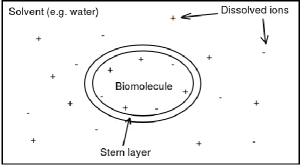
Figure 1: 2-D view of Debye-Hückel model.

This paper is an extension of the ECCOMAS Congress 2016 proceedings paper, Kweyu et al. (2016) with the following additional key inputs. Firstly, we employ nonaffine Dirichlet boundary conditions given in Section II.4 to replace the zero Dirichlet boundary conditions in the former. Secondly, and as a consequence of the nonaffine parameter dependence of these boundary conditions, we apply the discrete empirical interpolation method (DEIM) to reduce the resultant complexity in the reduced order model (ROM) during the online phase of the reduced basis method (RBM), see Section III.2 and Section III.3 Chaturantabut and Sorensen (2010). Lastly, we apply finite volume discretization to the dielectric coefficient function instead of taking the averages of the dielectric values between two neighbouring grid points. This is meant to reduce the truncation error as explained in Section II.2.

I.2 An overview of Poisson-Boltzmann Theory

There are numerous ways and reviews on the derivation of the PBE. The simplest stems from the Poisson equation Jackson (1975); Neves-Petersen and Petersen (2003) (in SI units),

$$-\vec{\nabla}.(\epsilon(x)\vec{\nabla}u(x))=\rho(x),\quad\textrm{in}\quad\Omega\in\mathbb{R}^{3},$$ (1)

which describes the electrostatic potential $u(x)$ at a point $x\in\Omega$. The term $\rho(x)$ is the charge distribution which generates the potential in a region with a position-dependent and piecewise constant dielectric function $\epsilon(x)$. Equation (1) is generally solved in a finite domain $\Omega$ subject to Dirichlet boundary conditions $u(x)=g(x)$ on $\partial{\Omega}$. Usually, $g(x)$ employs an analytic and asymptotically correct form of the electrostatic potential and therefore, the domain must be sufficiently large to ensure an accurate approximation of the boundary conditions Dong, Oslen, and Baker (2008).

To obtain the PBE from equation (1), we consider two contributions to the charge distribution $\rho(x)$: the “fixed” solute charges $\rho_{f}(x)$ and the aqueous “mobile” ions in the solvent $\rho_{m}(x)$. The $N_{m}$ partial atomic point charges ($z_{i}$) of the biomolecule are modeled as a sum of delta distributions at each atomic center $x_{i}$, for $i=1,\ldots,N_{m}$, that is,

$$\rho_{f}(x)=\frac{4\pi e^{2}}{k_{B}T}\sum_{i=1}^{N_{m}}z_{i}\delta(x-x_{i}).$$ (2)

The term $e/{k_{B}T}$ is the scaling coefficient which ensures that the electrostatic potential is dimensionless, where $e$ is the electron charge and $k_{B}T$ is the thermal energy of the system and is comprised of the Boltzmann constant $k_{B}$ and the absolute temperature $T$. The total charge of each atom is $ez_{i}$.

On the other hand, the solvent is modeled as a continuum through the Boltzmann distribution which leads to the mobile ion charge distribution

$$\rho_{m}(x)=\frac{4\pi e^{2}}{k_{B}T}\sum_{j=1}^{m}c_{j}q_{j}e^{-q_{j}u(x)-V_{j}(x)},$$ (3)

where we have $m$ mobile ion species with charges $q_{j}$ and bulk concentrations $c_{j}$. The term $V_{j}(x)$ is the steric potential which prevents an overlap between the biomolecule and the counterions. For monovalent electrolytes, whose ions are in a $1:1$ ratio, for example, $NaCl$, equation (3) reduces to

$$\rho_{m}(x)=-\kappa^{2}(x)\sinh(u(x)),$$ (4)

where the kappa function $\kappa^{2}(x)$ is position-dependent and piecewise constant; it describes both the ion accessibility through $e^{-V(x)}$ and the bulk ionic strength (or concentration) Baker (2005).

We eventually obtain the PBE by combining the two expressions for the charge distributions in (2) and (4) with the Poisson equation (1) for a monovalent electrolyte,

$$-\vec{\nabla}.(\epsilon(x)\vec{\nabla}u(x))+\bar{\kappa}^{2}(x)\sinh(u(x))=\frac{4\pi e^{2}}{k_{B}T}\sum_{i=1}^{N_{m}}z_{i}\delta(x-x_{i}),\quad\textrm{in}\quad\Omega\in\mathbb{R}^{3},$$ (5)

subject to

$$u(x)=g(x)\quad\textrm{on}\quad\partial{\Omega},$$ (6)

where

$$u(\infty)=0\,\implies u(x_{\max})\rightarrow 0\,\,\textrm{as}\,\,\left|x_{\max}\right|\rightarrow\infty.$$ (7)

In equation (5), $u(x)={e\psi(x)}/{k_{B}T}$ is the dimensionless potential scaled by $e/{k_{B}T}$ and $\psi(x)$ is the original electrostatic potential in centimeter-gram-second (cgs) units at $x\in\mathbb{R}^{3}$. The terms $\epsilon(x)$ and $\bar{k}^{2}(x)$ are discontinuous functions at the interface between the charged biomolecule and the solvent, and at an ion exclusion region (Stern layer) surrounding the molecule, respectively. The term $k^{2}={8\pi e^{2}I}/{1000\epsilon k_{B}T}$ is a function of the ionic strength $I=1/2\sum_{i=1}^{N}c_{i}z_{i}^{2}$. The function $g(x)$ represents the Dirichlet boundary conditions which are discussed in detail in Section II.4 and are nonaffine in the parameter $I$. Equation (7) shows that the electrostatic potential decays to zero exponentially as the position approaches infinity. Details on mapping $\epsilon(x)$ and $\bar{k}^{2}(x)$ onto a computational grid can be found in Baker, Holst, and Wang (2001). The PBE (5) poses severe computational challenges in both analytical and numerical approaches due to the infinite (unbounded) domain in (7), delta distributions, rapid nonlinearity, and discontinuous coefficients Holst (1994); Holst, Baker, and Wang (2000).

The PBE (5) can be linearized under the assumption that the electrostatic potential is very small relative to the thermal energy $k_{B}T$ Fogolari, Brigo, and Molinari (2002). Therefore, the nonlinear function $\textrm{sinh}(u(x))$ can be expanded into a Taylor series

$$\sinh(u(x))=u(x)+\frac{u(x)^{3}}{3!}+\frac{u(x)^{5}}{5!}+\ldots,$$ (8)

and only the first term is retained. We obtain the linearized PBE (LPBE) given by

$$-\vec{\nabla}.(\epsilon(x)\vec{\nabla}u(x))+\bar{k}^{2}(x)u(x)=(\frac{4\pi e^{2}}{k_{B}T})\sum_{i=1}^{N_{m}}z_{i}\delta(x-x_{i}).$$ (9)

Usually, proteins are not highly charged, and it suffices to consider the linearized PBE (LPBE). One can still obtain accurate results because the higher order terms in (8) do not provide a significant contribution. However, we must note that the LPBE can give inaccurate results for highly charged biomolecules such as the DNA and RNA (nucleic acids), phospholipid membranes, and polylysine Honig and Nicholls (1995). More information about the PBE, including its derivation from first principles, can be found in Holst (1994).

It is worth noting that there are recent developments of the PBE theory. Firstly, the biomolecular system has been considered as an interface problem which requires solution decomposition techniques to get rid of the solution singularities caused by the Dirac-delta distributions on the right hand side of (9) or (5). This has been discussed, for example, in L.Chen, Holst, and Xu (2009); Xie (2014); Xie and Ying (2016) where the LPBE has been modified into the form

$$\left.\begin{aligned} \begin{aligned} -\epsilon_{p}\Delta u(x)=\alpha\sum_{i=1}^{N_{m}}z_{i}\delta(x-x_{i}),\quad&x\in D_{p},\\ -\epsilon_{s}\Delta u(x)+\kappa^{2}u(x)=0,\quad&x\in D_{s},\\ u(s^{+})=u(s^{-}),\quad\epsilon_{s}\frac{\partial u(s^{+})}{\partial n(s)}=\epsilon_{p}\frac{\partial u(s^{-})}{\partial n(s)},\quad&s\in\varGamma,\\ u(s)=g(s),\quad&s\in\partial\Omega,\quad\end{aligned}\end{aligned}\right\}$$ (10)

where $\alpha$ is a constant, $D_{p}$ the protein domain, $D_{s}$ the solvent domain and $\varGamma$ the interface between the protein and the solvent. The PBE (nonlinear) has also been extensively solved as an interface problem L.Chen, Holst, and Xu (2009); Xie (2014).

The interface problem in (10) is more accurate than the model in (9) considered in this study, because the local or short-range potentials generated by the Dirac-delta distributions are computed independent of the long-range potentials, thus avoiding errors. However, this model is still computationally expensive because the numerical calculations by conventional methods are in $\mathcal{O}(\mathcal{N}^{3})$, (commonly known as the “curse of dimensionality”), where $\mathcal{N}$ is the dimension of the system in one direction. Therefore, we use the simple model (9) for the purpose of introducing and validating the RBM. Considering the interface problem would be our next step.

Secondly, studies on a variational problem of minimizing a mean-field variational electrostatic free-energy functional have been conducted Li, Wen, and Zhou (2016). This has been done in order to investigate the dependence of dielectric coefficient on local ionic concentrations and its effect on the equilibrium properties of electrostatic interactions in an ionic solution which was proposed, for instance, in Sala, Guadia, and Marti (2010). Results show that indeed the dielectric coefficient depends on the local ionic concentrations and this dependence can be expressed as a mathematical function which is continuous, monotonically decreasing, and convex Li, Wen, and Zhou (2016).

I.3 Applications and Post-processing of the PBE solution

The resultant electrostatic potential for the entire system can be used to calculate electrostatic free energies and electrostatic forces. The electrostatic free energy represents the work needed to assemble the biomolecule and is obtained by integration of the potential over a given domain of interest Vergara-Perez and Marucho (2016); Dong, Oslen, and Baker (2008). For the LPBE, this energy is given by

$$G_{elec}[u(x)]=\frac{1}{2}\int_{\Omega}\rho_{f}u(x)dx=\frac{1}{2}\sum_{i=1}^{N}z_{i}u(x_{i}),$$ (11)

where $u(x_{i})$ is the mean electrostatic potential acting on an atom $i$ located at position $x_{i}$ and carrying a charge $z_{i}$. The integral in (11) can be seen as the integral of polarization energy which is equivalent to the sum of interactions between charges and their respective potentials. On the other hand, it is also possible to differentiate the energy functional in (11) with respect to atomic positions to obtain the electrostatic force on each atom Gilson et al. (1993); Baker (2005); Dong, Oslen, and Baker (2008).

The electrostatic potential can also be evaluated on the surface of the biomolecule (electrostatic surface potential). It is used to provide information about the interaction between the biomolecule and other biomolecules or ligands or ions in its vicinity. Figure 2 shows the electrostatic potential mapped onto the surface of the protein fasciculin 1 and was generated by the Visual Molecular Dynamics (VMD) software at different orientations Humphrey, Dalke, and Schulten (1996). The electrostatic potential is computed by our FDM solver. The red colour represents regions of negative potential, the blue colour represents regions of positive potential, and the white colour represents neutral regions.

Figure 2: Electrostatic potential mapped onto protein
surface of fasciculin 1 toxin CPDB entry 1FAS.

The outline of this paper is as follows: In Section II, we provide a glimpse on the finite difference discretization of the LPBE and those of the dielectric coefficient and kappa functions, charge densities, as well as their respective mappings to the computational grid. In Section III, we provide the basics of the RBM which include the problem formulation, the solution manifold, the greedy algorithm, the discrete empirical interpolation method (DEIM), and the a posteriori error estimation. In Section IV, we provide numerical results of the FOM (via the FDM) and those of the ROM (via RBM and DEIM). Conclusions and some ideas on future work are given in the end.

II Discretization of the Poisson-Boltzmann Equation

II.1 Finite Difference Discretization

We discretize the LPBE in (2) with a centered finite differences scheme to obtain the algebraic linear system as below,

$$-\frac{H}{dx^{2}}\epsilon_{i+\frac{1}{2},j,k}^{x}(u_{i+1,j,k}-u_{i,j,k})+\frac{H}{dx^{2}}\epsilon_{i-\frac{1}{2},j,k}^{x}(u_{i,j,k}-u_{i-1,j,k})\\ -\frac{H}{dy^{2}}\epsilon_{i,j+\frac{1}{2},k}^{y}(u_{i,j+1,k}-u_{i,j,k})+\frac{H}{dy^{2}}\epsilon_{i,j-\frac{1}{2},k}^{y}(u_{i,j,k}-u_{i,j-1,k})\\ -\frac{H}{dz^{2}}\epsilon_{i,j,k+\frac{1}{2}}^{z}(u_{i,j,k+1}-u_{i,j,k})+\frac{H}{dz^{2}}\epsilon_{i,j,k-\frac{1}{2}}^{z}(u_{i,j,k}-u_{i,j,k-1})\\ +H\bar{\kappa}^{2}_{i,j,k}u_{i,j,k}=HCq_{i,j,k},$$ (12)

where $H=dx\times dy\times dz$ is a scaling factor, $q_{i,j,k}$ is the discretized molecular charge density and $C={4\pi e^{2}}/{k_{B}T}$. It is important to choose efficient algorithms and parameters to be used in the discretization of the charge density distribution, the kappa, and the dielectric functions that appear in the LPBE for the accuracy of the mean electrostatic potential solution. An efficient method is usually chosen to partition the domain into regions of solute (or biomolecule) and the solvent dielectric. Some of the key methods employed in APBS are the molecular surface and cubic-spline surface methods Vergara-Perez and Marucho (2016). In the following subsections, we provide some insights into these discretizations.

II.2 Calculation of Dielectric Constant Distribution and Kappa function

We notice that the dielectric constant $\epsilon$ in equation (12), is discretized at half grid, and therefore, we use a staggered mesh which results in three arrays (in $x$, $y$, and $z$ directions) representing the shifted dielectric values on different grids. This intends to fully take advantage of the finite volume discretization in order to minimize the solution error by increasing the spatial resolution. The dielectric coefficients and kappa functions which are piecewise constant, are mapped according to the following conditions,

$$\epsilon(x)=\begin{cases}2&\text{if }x\in\Omega_{1}\\ 78.54&\text{if }x\in\Omega_{2}\,\,\text{or}\,\,\Omega_{3}\end{cases},$$ (13)

$$\bar{k}(x)=\begin{cases}0&\text{if }x\in\Omega_{1}\,\,\text{or}\,\,\Omega_{2}\\ \sqrt{\epsilon_{3}}k&\text{if }x\in\Omega_{3}\end{cases},$$ (14)

where $\Omega_{1}$ is the region occupied by the protein molecule, $\Omega_{2}$ is the ion-exclusion layer, and $\Omega_{3}$ is the region occupied by the ionic solution.

Techniques used to map the dielectric and kappa functions onto the grid include, among others, the molecular surface, and the smoothed molecular surface, which are calculated using the Connolly approach Connolly (1983) and the cubic-spline surface. For more information see Vergara-Perez and Marucho (2016). The cubic-spline surface method, which is our method of choice, is more suitable than the other two because it is possible to evaluate the gradient of the mean electrostatic potential such as in the determination of the solvated or polar forces. This method introduces an intermediate dielectric region at the interface between the solute and the solvent because the kappa and dielectric maps are built on a cubic-spline surface. This smoothes the transition of the functions to circumvent discontinuities inherent in them Baker, Holst, and Wang (2001); Vergara-Perez and Marucho (2016).

II.3 Calculation of Charge Densities

The molecular charge density (right-hand side of the LPBE (9)) can be obtained from any file with atomic coordinates, charges, and radii. However, these atomic coordinates may not coincide with any of our grid points. Therefore, it is necessary to find an efficient method of spreading the point charges (summation term in LPBE) to the grid points. Several methods are available to map or spread the charges onto the grid points, e.g. in the APBS software package. Trilinear interpolation (or linear spline) in which charges are mapped onto nearest-neighbour grids, results in potentials which are very sensitive to the grid resolution. Cubic B-spline interpolation where charges are mapped to two layers of grid points, has an average sensitivity to the grid setup, and quintic B-spline interpolation has the lowest sensitivity to grid spacing because charges are spread out to three layers of the grid points Baker, Holst, and Wang (2001).

In this study, we use the cubic B-spline interpolation (basis spline) method which maps the charges to the nearest and next-nearest grid points. Although computationally expensive, this method provides softer or smoother distributions of charges which subsequently reduces the sensitivity of the mean electrostatic potential solutions to the grid spacing Vergara-Perez and Marucho (2016).

II.4 Dirichlet Boundary Conditions

Analytical solutions to the LPBE can only be obtained for systems with simple geometries, for example, spherical and cylindrical systems. Equation (15) shows an analytical solution for a spherical molecule with uniform charge (Born ion) Holst (1994). From this equation, we can obtain two different kinds of Dirichlet boundary conditions, the single Debye-Hückel (SDH) and multiple Debye-Hückel (MDH). For the former, we assume that all the atomic charges are collected into a single charge at the center of the solute approximated by a sphere. This kind of boundary condition is suitable when the boundary is sufficiently far from the biomolecule. On the other hand, the latter assumes the superposition of the contribution of each atomic charge (i.e. multiple, non-interacting spheres with point charges) with respective radius. This kind of boundary condition is more accurate than SDH for closer boundaries but can be computationally expensive for large biomolecules.

In this study, we employ the MDH type Baker, Holst, and Wang (2001); Rocchia (2005),

$$u(x)=(\frac{e^{2}}{k_{B}T})\sum\limits_{i=1}^{Nm}\frac{z_{i}e^{-\kappa(d-a_{i})}}{\epsilon_{w}(1+ka_{i})d}\quad\textrm{on}\quad\partial{\Omega},\quad d=\lvert x-x_{i}\rvert.$$ (15)

Here, $z_{i}$ are the point partial charges of the protein, $\epsilon_{w}$ is the solvent dielectric, $\kappa=\bar{\kappa}/\sqrt{\epsilon_{w}}$ is a function of the ionic strength of the solution, $a_{i}$ are the atomic radii, and $N_{m}$ is the total number of point partial charges in the protein.

III Essentials of the Reduced Basis Method

The Reduced basis method (RBM) and proper orthogonal decomposition (POD) are examples of popular projection-based parametrized model order reduction (PMOR) techniques. The main goal of these techniques is to generate a parametric ROM which accurately approximates the original full order model (FOM) of high dimension over varying parameter values Benner, Gugercin, and Willcox (2015); Eftang (2011); Rozza, Huynh, and Patera (2008). The RBM exploits an offline/online procedure which ensures an accurate approximation of the high-fidelity solution in a rapid and inexpensive manner and is widely applicable in real-time and many-query scenarios. For a thorough review, see Benner, Gugercin, and Willcox (2015).

We consider a physical domain $\Omega\subset\mathbb{R}^{3}$ with boundary $\partial\Omega$, and a parameter domain $D\subset\mathbb{R}$. The LPBE (9) is discretized with the centered finite difference scheme (12) on $\Omega$ and Dirichlet boundary conditions (6) obtained from (15) are applied. The resultant discrete problem of the LPBE becomes, for any $\mu\in D$, find $u^{\mathcal{N}}(\mu)$ that satisfies the linear system

$$A(\mu)u^{\mathcal{N}}(\mu)=f(\mu),\quad\mu\in D,$$ (16)

where $A(\mu)\in\mathbb{R}^{\mathcal{N}\times\mathcal{N}}$ and $f(\mu)\in\mathbb{R}^{\mathcal{N}}$. The matrix $A(\mu)$ can also be written as a parameter-affine matrix,

$$A(\mu)=\sum\limits_{i=1}^{Q}\Theta_{i}(\mu)A_{i},$$ (17)

where $Q\in\mathbb{N}$, $\Theta_{i}$ are scalar coefficient functions, and $A_{i}$ are the parameter independent matrices. The $\mathcal{N}\times\mathcal{N}$ system is indeed computationally expensive to be solved for an accurate approximation of $u(\mu)$ because the dimension $\mathcal{N}$ is approximately $2\times 10^{6}$ in our problem. Therefore, we apply the RBM to save computational costs by providing an accurate approximation of $u^{\mathcal{N}}(\mu)$ at a greatly reduced dimension of $N\ll\mathcal{N}$. The ROM is given by (20).

However, as detailed in Section III.2, we encounter some computational complexity in the online phase of RBM which is caused by the nonaffine parameter dependence in the right-hand side vector $f(\mu)$ from the boundary condition (15). The parameter, the ionic strength, resides in the kappa term $\kappa$ in the exponential function. This violates one of the key assumptions of the RBM which requires that all the system matrices and vectors must be affinely dependent on the parameter so that the offline/online decomposition is natural Hesthaven, Rozza, and Stamm (2016). To circumvent this problem, we propose to apply an empirical interpolation method to reduce the complexity of the the online phase by avoiding the high-dimensional computation related to the vector $f(\mu)$. We provide some details in Section III.3.

III.1 The Solution Manifold and the Greedy Algorithm

Another key assumption in RBM besides the affine parameter dependence, is the existence of a typically smooth and very low dimensional solution manifold which almost covers all the high-fidelity solutions of (16) under variation of parameters Eftang (2011),

$$\mathcal{M}^{\mathcal{N}}=\{u^{\mathcal{N}}(\mu):\mu\in D\}.$$ (18)

The RB approximation space is then built upon this solution manifold and is given by the subspace spanned by the snapshots of the FOM. In other words, it is the subspace spanned by the high-fidelity $u^{\mathcal{N}}(\mu)$ solutions corresponding to a number of samples of the parameters, that is,

$$\textrm{range}(V)=\textrm{span}\{u^{\mathcal{N}}(\mu_{1}),...,u^{\mathcal{N}}(\mu_{l})\},\quad\forall\mu_{1},...,\mu_{l}\in D.$$ (19)

The greedy algorithm as given in Algorithm 1 is used to generate the reduced basis space (19) through an iterative procedure where a new basis is computed at each iteration Hess and Benner (2013). The RB space can be thought of being nested or hierarchical such that the previous basis set is a subset of the next and so on.

Algorithm 1 Greedy algorithmHesthaven, Stamm, and Zhang (2014)

1:A training set $\Xi\subset D$ including samples of $\mu$ covering the parameter domain $D$, i.e., $\Xi:=\{\mu_{1},\ldots,\mu_{l}\}$.

2:RB basis represented by the projection matrix $V$.

3:Choose $\mu^{*}\in\Xi$ arbitrarily.

4:Solve FOM (16) for $u^{\mathcal{N}}(\mu^{*})$.

5:$V_{1}=[u^{\mathcal{N}}(\mu^{*})]$, $N=1$.

6:while $\max\limits_{\mu\in\Xi}\Delta_{N}(\mu)\geq\epsilon$ do

7:     $\mu^{*}=\textrm{arg}\max\limits_{\mu\in\Xi}\Delta_{N}(\mu)$.

8:     Solve FOM (16) for $u^{\mathcal{N}}(\mu^{*})$.

9:     $V_{N+1}=[V_{N}\quad u^{\mathcal{N}}(\mu^{*})]$.

10:     Orthonormalize the columns of $V_{N+1}$.

11:     $N=N+1$.

12:end while

The RB approximation is then formulated as, for any given $\mu\in D$, find $u_{N}(\mu)\in X_{N}$ which satisfies

$$A_{N}(\mu)u_{N}(\mu)=f_{N}(\mu),$$ (20)

where $A_{N}=V^{T}AV$ and $f_{N}(\mu)=V^{T}f(\mu)$. $V$ is the orthonormal matrix computed from the greedy algorithm. From the fact that $N\ll\mathcal{N}$, solving the small dimensional reduced order model (ROM) is much cheaper than solving the high-fidelity model, the FOM (16) Eftang (2011). However, one problem still remains when computing the ROM. The computational complexity of evaluating the nonaffine function $f_{N}(\mu)$ still depends on the dimension of the FOM, as illustrated in Section III.2. Efficient implementation of Algorithm 1 depends on an efficient error estimation $\Delta_{N}(\mu)$ of the ROM, which is discussed in Section III.5.

III.2 Computational Complexity of the Reduced Order Model (ROM)

To demystify the issue of computational complexity in the ROM, we can first rewrite (16) explicitly to illustrate the affine parameter decomposition on the left-hand side and the nonaffine right-hand side,

$$(A_{1}+\mu A_{2})u^{\mathcal{N}}=\rho+b(\mu),\quad\mu\in D,$$ (21)

where the matrix $A_{1}$ comes from the Laplacian operator term, $A_{2}$ is a diagonal matrix from the $kappa$ term, $\rho$ represents the charge density term and $b(\mu)$, the boundary conditions obtained from the analytical solution in (15). We can clearly notice the affine parameter decomposition of the matrix $A$ in (16) into $A_{1}$ and $\mu A_{2}$ in (21). However, the right-hand side function $b(\mu)$ is nonaffine in the parameter and therefore it cannot be decomposed in such a manner. Consider the ROM which is obtained by the greedy algorithm approach in Algorithm 1 and a Galerkin projection,

$$(\underbrace{\hat{A_{1}}}_{N\times N}+\mu\underbrace{\hat{A_{2}}}_{N\times N})\underbrace{u^{N}}_{N\times 1}=\underbrace{\hat{\rho}}_{N\times 1}+\underbrace{V^{T}}_{N\times\mathcal{N}}\underbrace{b(\mu)}_{\mathcal{N}\times 1},$$ (22)

where $\hat{A_{1}}=V^{T}A_{1}V$, $\hat{A_{2}}=V^{T}A_{2}V$, $\hat{\rho}=V^{T}\rho$, and $N\ll\mathcal{N}$.

It is clear from (22) that the last term of the right-hand side (RHS) still depends on the dimension $\mathcal{N}$ of the FOM while all the other matrices and vectors depend only on the dimension $N$ of the ROM, with $N\ll\mathcal{N}$. Therefore, the reduced order matrices on the left-hand side and the first vector on the right-hand side of (22) can be precomputed and stored during the offline phase, thereby providing a lot of computational savings. However, the term $V^{T}b(\mu)$ cannot be precomputed because of the aforementioned nonaffine parameter dependence and therefore, the Galerkin projection involving matrix-vector products which are dependent on the dimension $\mathcal{N}$, has to be computed in the online phase of solving the ROM.

In principle, we require $\mathcal{O}(2\mathcal{N}N)$ flops for these matrix-vector products and a full evaluation of the nonaffine analytical function (15) to obtain $V^{T}b(\mu)$. This can be computationally expensive for a large $\mathcal{N}$, especially during the a posteriori error estimation (computing $\Delta_{N}(\mu)$), where the residual is computed $l$ times for varying parameter values $\mu_{i}$, $i=1,\ldots,l$ for a single iteration of the greedy algorithm. The discrete empirical interpolation method (DEIM) is an approach to circumvent this problem in order to reduce the computational complexity of the nonaffine function. We discuss this technique at length in the next Subsection.

III.3 Discrete Empirical Interpolation Method (DEIM)

DEIM is a complexity reduction technique that was proposed in Chaturantabut and Sorensen (2010) to overcome the drawback of the proper orthogonal decomposition (POD) approach for approximating a nonaffine (or nonlinear) parametrized function in the ROM during the online phase. This drawback is in the sense that the evaluation of the nonlinear/nonaffine function is still equivalent to that of computing the counterpart of the original system, which yields no computational savings. Therefore, the main idea of DEIM is to interpolate the nonlinear/nonaffine function by computing only a few entries of it, which dramatically reduces the computational complexity Chaturantabut and Sorensen (2010); Wirtz, Sorensen, and Haasdonk (2014).

We provide a brief overview on using the singular value decomposition (SVD) to obtain the interpolation basis vectors. Firstly, we compute snapshots of the function $b(\mu)$ at a set of parameter $\mu$ in the training set $\Xi=\{\mu_{1},\ldots,\mu_{l}\}\subset D$ and construct the snapshot matrix,

$$F=[b(\mu_{1}),\ldots,b(\mu_{l})]\in\mathbb{R}^{\mathcal{N}\times l}.$$ (23)

Secondly, we compute its singular value decomposition (SVD),

$$F=U_{F}\Sigma W^{T},$$ (24)

where $U_{F}\in\mathbb{R}^{\mathcal{N}\times l}$, $\Sigma\in\mathbb{R}^{l\times l}$, and $W\in\mathbb{R}^{l\times l}$. Note that the matrices $U_{F}$ and $W$ are orthogonal, that is, $(U_{F})^{T}U_{F}=W^{T}W=I_{l}$, $I_{l}\in\mathbb{R}^{l\times l}$ and $\Sigma=\textrm{diag}(\sigma_{1},\ldots,\sigma_{l})$, with $\sigma_{1}\geq\ldots\geq\sigma_{l}\geq 0$.

Figure 3 shows the decay of the singular values of $\Sigma$ for the protein fasciculin 1. Figure 3(a) shows the behaviour of $20$ singular values with almost no decay from the $11th$ singular value. We discard these non-decaying singular values to obtain those in Figure 3(b). From the latter, we can actually truncate the singular values by selecting only the largest of them represented by $r\in\{1,\ldots,l\}$ that correspond to some required degree of accuracy. In this case, $l=11$ and $r=9$ which corresponds to an accuracy of $\epsilon_{svd}=O(10^{-10})$ in (26). The number $r$ plays an important role to select a basis set $\{u_{i}^{F}\}_{i=1}^{r}$ of rank $r$ from $U_{F}$ which solves the minimization problem Volkwein (2013),

$$\textrm{arg}\min\limits_{\{\tilde{u}_{i}\}_{i=1}^{r}}\sum_{j=1}^{l}\Arrowvert F_{j}-\sum_{i=1}^{r}\langle F_{j},\tilde{u}_{i}\rangle\tilde{u}_{i}\Arrowvert_{2}^{2},\quad\text{s.t.}\,\langle\tilde{u}_{i},\tilde{u}_{j}\rangle=\delta_{ij},$$ (25)

where $F_{j}$ is the $j$th column of the snapshot matrix $F$, and $\delta_{ij}$ is the usual Kronecker delta.

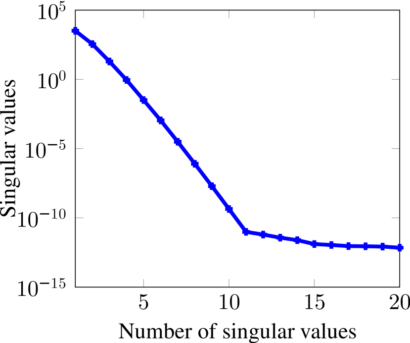
(a) 20 singular values

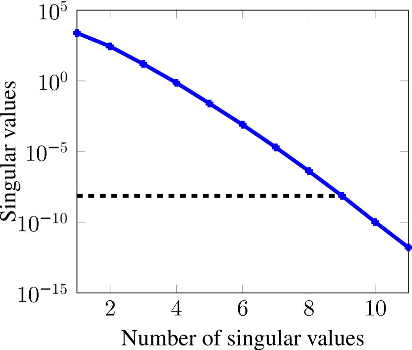
(b) 11 singular values

Figure 3: Decay of singular values of $\Sigma$ in (24).

The following criterion is used to truncate the largest singular values from Figure 3 based on some desired accuracy, $\epsilon_{svd}$.

$$\frac{\sum\limits_{i=r+1}^{l}\sigma_{i}}{\sum\limits_{1=1}^{l}\sigma_{i}}<\epsilon_{svd},$$ (26)

where $\sigma_{i},i=1,\ldots,l$ are the nonzero singular values of $F$. The dotted horizontal black line corresponds to $r=9$ singular values and the corresponding singular vectors $\{u_{i}^{F}\}_{i=1}^{r}$ are used in the DEIM approximation.

DEIM overcomes the problem mentioned in Section III.2 by determining an interpolation of the nonaffine function $b(\mu)$. This is realized by approximating $b(\mu)$ with the linear combination of the basis vectors $U_{F}=[u_{1}^{F},\ldots,u_{r}^{F}]\in\mathbb{R}^{\mathcal{N}\times r}$, i.e.

$$b(\mu)\approx U_{F}c(\mu),$$ (27)

where $c(\mu)\in\mathbb{R}^{r}$ is the corresponding coefficient vector, and can be determined by assuming that $U_{F}c(\mu)$ interpolates $b(\mu)$ at $r$ selected interpolation points, then,

$$P^{T}b(\mu)=P^{T}U_{F}c(\mu),$$ (28)

where $P$ is an index matrix given by

$$P=[e_{\wp_{1}},\ldots,e_{\wp_{r}}]\in\mathbb{R}^{\mathcal{N}\times r},$$ (29)

which consists of unit vectors $e_{\wp_{i}}$, $i=1,\ldots,r$, where the indices $\wp_{i}$, are the DEIM interpolation points which are selected iteratively with a greedy algorithm. Suppose that $P^{T}U_{F}\in\mathbb{R}^{r\times r}$ is nondegenerate, then $c(\mu)$ can be determined from (28) by

$$c(\mu)=(P^{T}U_{F})^{-1}P^{T}b(\mu).$$ (30)

Therefore, the function $b(\mu)$ in (14) can be approximated as

$$b(\mu)\approx U_{F}c(\mu)=U_{F}(P^{T}U_{F})^{-1}P^{T}b(\mu),$$ (31)

so that the ROM in (22) with DEIM approximation becomes,

$$(\underbrace{\hat{A_{1}}}_{N\times N}+\mu\underbrace{\hat{A_{2}}}_{N\times N})\underbrace{u^{N}(\mu)}_{N\times 1}=\underbrace{\hat{\rho}}_{N\times 1}+\underbrace{V^{T}U_{F}(P^{T}U_{F})^{-1}}_{N\times r}\underbrace{P^{T}b(\mu)}_{r\times 1}.$$ (32)

The interpolant $V^{T}U_{F}(P^{T}U_{F})^{-1}P^{T}b(\mu)$ can be computed a lot cheaper than $V^{T}b(\mu)$ because we can precompute $V^{T}U_{F}(P^{T}U_{F})^{-1}$ independent of the parameter $\mu$. Alternatively, we can also compute only those entries in $b(\mu)$ that correspond to the interpolation indices $\wp_{i},i=1,\ldots,r$, $r\ll\mathcal{N}$, i.e., $P^{T}b(\mu)$ instead of the entire $\mathcal{N}$ entries in $b(\mu)$.

For the actual numerical implementation of the interpolation (31), the matrix $P$ needs not be explicitly applied. Instead, only the interpolation indices $\wp_{i},i=1,\ldots,r$ need to be applied to the matrix $U_{F}$ or the nonaffine function $b(\mu)$. This implies that $P^{T}U_{F}$ merely consists of the rows of $U_{F}$ which correspond to the interpolation indices $\wp_{i},i=1,\ldots,r$. Similarly, $P^{T}b(\mu)$ is a condensed vector composed of a few entries of $b(\mu)$ which correspond to the same indices.

Algorithm 2 provides a brief overview of the DEIM procedure.

Algorithm 2 DEIM algorithm Chaturantabut and Sorensen (2010); Feng, Mangold, and Benner (2017)

1:POD basis $\{u_{i}^{F}\}_{i=1}^{r}$ for $F$ in equation (10).

2:DEIM basis $U_{F}$ and indices $\vec{\wp}=[\wp_{1},\ldots,\wp_{r}]^{T}\in\mathbb{R}^{r}$.

3:$\wp_{1}$ = $\textrm{arg}\max\limits_{j\in\{1,\ldots,\mathcal{N}\}}\lvert u_{1j}^{F}\rvert$, where $u_{1}^{F}=(u_{11}^{F},\ldots,u_{1\mathcal{N}}^{F})^{T}$.

4:$U_{F}=[u_{1}^{F}]$, $P=[e_{\wp_{1}}],\vec{\wp}=[\wp_{1}]$.

5:for i = 2 to r do

6:     Solve $(P^{T}U_{F})\alpha=P^{T}u_{i}^{F}$ for $\alpha$, where $\alpha=(\alpha_{1},\ldots,\alpha_{i-1})^{T}$,

7:     $r_{i}=u_{i}^{F}-U_{F}\alpha$,

8:     $\wp_{i}$ = $\textrm{arg}\max\limits_{j\in\{1,\ldots,\mathcal{N}\}}\lvert r_{ij}\rvert$, where $r_{i}=(r_{i1},\ldots,r_{i\mathcal{N}})^{T}$.

9:     $U_{F}\leftarrow[U_{F}\ u_{i}^{F}]$, $P\leftarrow[P\ e_{\wp_{i}}]$, $\vec{\wp}\leftarrow\begin{bmatrix}\vec{\wp}\\ \wp_{i}\end{bmatrix}$.

10:end for

Note that in Algorithm 2, the POD basis $\{u_{i}^{F}\}_{i=1}^{r}$ is of great significance as an input basis for the DEIM procedure in two ways. First, a set of interpolation indices $\wp_{i}$ are constructed inductively based on this basis through a greedy algorithm. Secondly, an error analysis in Chaturantabut and Sorensen (2010) indicates that the ordering of this basis according to the dominant singular values makes it the right choice for this algorithm. In step 1, the process selects the first interpolation index $\wp_{1}$ which corresponds to the location of the entry in $u_{1}^{F}$ with the largest magnitude. The subsequent indices in step 6, $\wp_{i},i=2,\ldots,r$, are selected in such a way that each of them corresponds to the location of the entry in $r$ (step 5) with the largest magnitude.

III.4 DEIM Approximation Error

We compute the error due to the DEIM interpolation which is to be included into the residual in the a posteriori error estimation. This error was first proposed in Wirtz, Sorensen, and Haasdonk (2014) for nonlinear dynamical systems and has also been used in Feng, Mangold, and Benner (2017) in the context of a nonlinear population balance systems. We extend this idea to parametrized elliptic PDEs where the DEIM error is given by,

$$e_{\textrm{DEIM}}=b(\mu)-\tilde{b}(\mu)=\Pi_{2}(I-\Pi)b(\mu),$$ (33)

where $\Pi$ and $\Pi_{2}$ are oblique projectors defined as follows,

$$\Pi=U_{F}(P^{T}U_{F})^{-1}P^{T},$$ (34)

and

$$\Pi_{2}=(I-\Pi)\tilde{U}_{F}(\tilde{P}^{T}(I-\Pi)\tilde{U}_{F})^{-1}\tilde{P}^{T}.$$ (35)

In equation (34), $U_{F}=(u_{1}^{F},\ldots,u_{r}^{F})\in\mathbb{R}^{\mathcal{N}\times r}$ and $P\in\mathbb{R}^{\mathcal{N}\times r}$ are the current DEIM basis and interpolation index matrix obtained from Algorithm 2.

To obtain $\Pi_{2}$ in (35), we assume that $r^{*}(\geq r)$ DEIM basis vectors $U_{F}^{*}=(u_{1}^{F},\ldots,u_{r^{*}}^{F})$ interpolate $b(\mu)$ exactly, i.e.

$$b(\mu)=U_{F}^{*}((P^{*})^{T}U_{F}^{*})^{-1}(P^{*})^{T}b(\mu),$$ (36)

where $P^{*}$ is the corresponding index matrix with $r^{*}$ columns. Finally, $\tilde{U}_{F}=U_{F}^{*}(:,r+1:r^{*})$ and $\tilde{P}=P^{*}(:,r+1:r^{*})$ such that $U_{F}^{*}=[U_{F},\tilde{U}_{F}]$ and $P^{*}=[P,\tilde{P}]$, where $M(:,r+1:r^{*})$, using MATLAB notation Feng, Mangold, and Benner (2017). In the next subsection, we introduce an a posteriori error estimation derived from the residual of the approximate RB solution and the DEIM approximation error.

III.5 A Posteriori Error Estimation

A posteriori error estimators are computable indicators which provide an estimate to the actual solution error by utilizing the residual of the approximate RB solution. An efficient error estimator is required to possess three major characteristics, namely: it is required to be as sharp as possible (close to the unknown actual error), asymptotically correct (tend to zero with increasing RB space dimension $N$, at a similar rate as the actual error), and computationally cheap (because it is computed in the online phase). Therefore, these estimators guarantee both reliability and efficiency of the reduction process Quarteroni, Manzoni, and Negri (2016).

We first compute the residual due to DEIM interpolation;

$$r_{N}^{\textrm{DEIM}}(u_{N};\mu)=(\rho+\tilde{b}(\mu))-A^{\mathcal{N}}(\mu)u_{N}(\mu),$$ (37)

where $\tilde{b}(\mu)=\Pi b(\mu)$ is the DEIM interpolation of $b(\mu)$ and $u_{N}(\mu):=Vu^{N}(\mu)$ is the RB solution transformed back to the high-fidelity space $\mathcal{N}$. Then the final residual is obtained by including the DEIM approximation error derived in Section III.4 as follows;

$$\begin{split}r_{N}(u_{N};\mu)&=(\rho+b(\mu))-A^{\mathcal{N}}(\mu)u_{N}(\mu)\\ &=(\rho+\tilde{b}(\mu))-A^{\mathcal{N}}(\mu)u_{N}(\mu)+b(\mu)-\tilde{b}(\mu)\\ &=r_{N}^{\textrm{DEIM}}(u_{N};\mu)+\underbrace{b(\mu)-\tilde{b}(\mu)}_{:=e_{\textrm{DEIM}}}\\ &=r_{N}^{\textrm{DEIM}}(u_{N};\mu)+e_{\textrm{DEIM}}.\end{split}$$ (38)

The a posteriori error estimation is then derived from the residual in (38). Rewriting the first equation of (38), we obtain

$$\begin{split}r_{N}(u_{N};\mu)&=A^{\mathcal{N}}(\mu)u^{\mathcal{N}}(\mu)-A^{\mathcal{N}}(\mu)u_{N}(\mu)\\ &=A^{\mathcal{N}}(\mu)e(\mu),\end{split}$$ (39)

where the error $e(\mu):=u^{\mathcal{N}}(\mu)-u_{N}(\mu)$ is given by

$$e(\mu)=(A^{\mathcal{N}}(\mu))^{-1}r_{N}(u_{N};\mu).$$ (40)

We obtain an upper bound for the 2-norm of the error by taking the 2-norm on both sides of equation (40), i.e.

$$\begin{split}\Arrowvert e(\mu)\Arrowvert_{2}\leq\Arrowvert(A^{\mathcal{N}})^{-1}(\mu)\Arrowvert_{2}\Arrowvert r_{N}(u_{N};\mu)\Arrowvert_{2}&=\frac{\Arrowvert r_{N}(u_{N};\mu)\Arrowvert_{2}}{\sigma_{min}(A^{\mathcal{N}}(\mu))}\\ &=:\tilde{\Delta}_{N}(\mu),\end{split}$$ (41)

where $\sigma_{min}(A^{\mathcal{N}}(\mu))$ is the smallest singular value of $A^{\mathcal{N}}(\mu)$ Quarteroni, Manzoni, and Negri (2016). The quantity $\tilde{\Delta}_{N}(\mu)$ is a rigorous error bound, and can be used to select snapshots within the greedy algorithm in the offline stage and consequently to measure the accuracy of the RB approximation in the online stage Hess and Benner (2013). For efficient computation of the norm of the residual and error bounds, see Hesthaven, Rozza, and Stamm (2016); Quarteroni, Manzoni, and Negri (2016). It is computationally expensive to compute $\sigma_{min}(A^{\mathcal{N}}(\mu))$ in the online phase as it entails solutions of large-scale eigenvalue problems Hess and Benner (2013). Therefore, in our computations, we use the norm of the residual as our error estimator, which satisfies the inequality (41) and provides an estimation of the true error that works well for our problem. It also provides rapid convergence as depicted in the numerical results in Figure 5. It is given by

$$\Arrowvert e(\mu)\Arrowvert_{2}\approx\Arrowvert r_{N}(u_{N};\mu)\Arrowvert_{2}:=\Delta_{N}(\mu).$$ (42)

IV Numerical Results

IV.1 Finite Difference Results

We consider the LPBE (9), a parameter domain $\mu\in D=[0.05,0.15]$, and a cubic grid of $129$ points and a box length of $60\,\textrm{\AA}$ centered at the protein position. The parameter domain is chosen for a feasible physiological process and $\mu$ resides in the second term in the kappa function. Information about the molecular charge density is obtained from a PQR file which contains $1228$ atoms of the protein fasciculin 1 toxin CPDB entry 1FAS. We discretize the LPBE with a centered finite difference scheme and the resulting parametrized linear system (16) is of more than $2\times 10^{6}$ degrees of freedom. This FOM is solved by the aggregation-based algebraic multigrid (AGMG) method, where a tolerance of $10^{-10}$ and a zero initial guess are used Notay (2010); Napov and Notay (2012); Notay (2012).

The choice of the tolerance directly affects the results of the greedy algorithm. Therefore, it is prudent to ensure that the high-fidelity solution ($u^{\mathcal{N}}(\mu),\mathcal{N}=2,146,689$) is highly accurate. Some of the iterative methods commonly used in the PBE solvers are; the minimal residual (MINRES) method, the generalized minimal residual (GMRES) method and the biconjugate gradient stabilized (BICGSTAB) method. These methods employ the incomplete LU factorization to generate the preconditioner matrices L (lower diagonal) and U (upper diagonal) which are used to improve their stability and convergence at low costs Vergara-Perez and Marucho (2016).

Figure 4 shows the lower cross-sections of the $z$-axis of the electrostatic potential $u(x,y,1)$. Note that the potential decays exponentially with the variation of the parameter $\mu$, and is attributed to the large force constant ($332$ kcal/mol) of electrostatic interactions. In the absence of ions (that is, at $\mu=I=0$), these interactions are long ranged, but in the presence of ions (that is, $\mu>0$), they are damped or screened and gradually decay to zero Fogolari, Brigo, and Molinari (2002). The computational time taken to obtain the high-fidelity solution $u^{\mathcal{N}}(\mu)$ is approximately $28$ seconds on average and varies depending on the value of the ionic strength used.

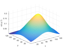
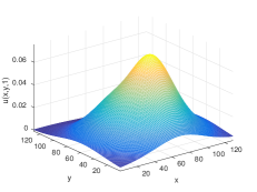
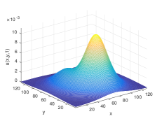
Figure 4: High-fidelity solutions ($u^{\mathcal{N}}(\mu)$) at varying ionic
strengths (i.e., $\mu$ = {0, 0.05, 0.15, 0.5}), respectivley.

IV.2 Accuracy of FDM

We demonstrate the accuracy and reliability of the FDM before applying the RBM for the solution of the PBE. This is because the accuracy of the RBM depends on that of the underlying discretization technique. In this study, we consider six test examples to validate the FDM which include a Born ion and five proteins consisting of between $380$ and $3400$ atoms, respectively. We compare the FDM results with those of APBS for electrostatic solvation free energy at different mesh refinements. Firstly, we consider the Born ion which is a canonical example for polar solvation and whose analytical solution is well known.

This analytical solution gives the polar solvation energy which results from the transfer of a non-polarizable ion between two dielectrics www , i.e.,

$$\Delta_{p}G_{Born}=\frac{q^{2}}{8\pi\epsilon_{0}r}(\frac{1}{\epsilon_{out}}-\frac{1}{\epsilon_{in}}),$$ (43)

where $q$ is the ion charge, $r$ is the ion radius, $\epsilon_{out}$ is the external dielectric coefficient (e.g., water) and $\epsilon_{in}$ is the internal dielectric coefficient (e.g., vacuum). This model assumes zero ionic strength. We consider a Born ion of unit charge, $3\textrm{\AA}$ radius and located at the origin ($(0,0,0)$). Here, $\epsilon_{in}=1$ and $\epsilon_{out}=78.54$. With these parameters, the analytical solution in (43) is

$$\Delta_{p}G_{Born}=-691.85(\frac{q^{2}}{r})=-230.62\textrm{kJ/mol}.$$ (44)

We compare numerical computations using equation (11) for charging free energies in a homogeneous ($\epsilon_{in}=\epsilon_{out}=1$) and heterogeneous ($\epsilon_{in}=1,\epsilon_{out}=78.54$) dielectric coefficients with the analytical solution www . We use the following additional parameters. We consider two different mesh sizes (or $\Delta x$), which result in different degrees of freedom (or $\mathcal{N}$) as shown in Table 1. Numerical results using FDM are compared with those of the exact solution (43) and APBS (which uses FEM). The results show that the FDM method gives solutions which are consistent with those of the exact solutions, as well as those of the APBS software package.

$\Delta x$	$\mathcal{N}$	Solver	Numerical	Analytical	Relative error
0.33	$97^{3}$	APBS	-229.59	-230.62	4.4662e-3
		FDM	-232.86	-230.62	9.7130e-3
0.25	$129^{3}$	APBS	-230.00	-230.62	2.6884e-3
		FDM	-230.42	-230.62	8.6723e-4

Table 1: Comparison of Born ion solvation energies in kJ/mol.

Secondly, we compare the accuracy of FDM for the LPBE with the following set of typical examples of use of LPBE and APBS in particular: Calculation of the total electrostatic energy (including self-interaction energies) of a $22$ residue, $\alpha$-helical peptide from the N protein of phage $\lambda$ which binds to its cognate $19$ nucleotide box B RNA hairpin Garcia-Garcia and Draper (2003), Fasciculin 1, an anti-acetylcholinesterase toxin from green mamba snake venom Le Du (1992), the electrostatic potential of a minimized FKBP protein from binding energy calculations of small ligands Burkhard, Taylor, and D. (2000), a 180-residue cytokine solution NMR structure of a murine-human chimera of leukemia inhibitory factor (LIF) Hinds et al. (1998), and the binding energy of a balanol ligand to the catalytic subunit of the CAMP-dependent protein kinase A, here the apo form of the enzyme Narayana et al. (1999). The proteins and or complexes have the following number of atoms (379, 1228, 1663, 2809, and 3423), respectively.

The electrostatic solvation free energies, $\Delta E$ are computed and shown in Table 2 for varying grid resolutions $\Delta x$. However, we here do not have the analytical electrostatic energies for these proteins but rely on the accuracy of the APBS software for validation. A compute cluster with 4 Intel Xeon E7-8837 CPUs running at 2.67 GHz (8 cores per CPU) and 1 TB RAM, split into four 256 GB parts (each CPU controls one part) is used to carry out the computations which require a huge amount of memory, so that it allows for solving large-scale problems with $\mathcal{N}\geq(3\times 10^{6})$.

$\Delta x$	$\mathcal{N}$	$\Delta E$, FDM	$\Delta E$, APBS	Relative error
1. Solvation energies of a $22$ residue, $\alpha$-helical peptide from the N protein of phage $\lambda$ in kJ/mol. (379 atoms)
0.375	$129^{3}$	-4557.7052	-4546.5150	2.4613e-3
0.320	$161^{3}$	-4541.4782	-4532.7595	1.9235e-3
0.260	$193^{3}$	-4522.4752	-4516.8544	1.2444e-3
2. Solvation energies of fasciculin 1 in kJ/mol. (1228 atoms)
0.465	$129^{3}$	-5870.5357	-5845.8594	4.2212e-3
0.375	$161^{3}$	-5684.8448	-5664.8475	3.5301e-3
0.320	$193^{3}$	-5629.1979	-5611.2503	3.1985e-3
3. Solvation energies of the electrostatic potential of a minimized FKBP protein in kJ/mol. (1663 atoms)
0.465	$129^{3}$	-4419.0384	-4403.8761	3.4429e-3
0.375	$193^{3}$	-4344.5491	-4331.1010	3.1050e-3
0.320	$225^{3}$	-4292.5359	-4288.0842	1.0382e-3
4. Solvation energies of a 180-residue cytokine solution NMR structure of a murine-human chimera of leukemia inhibitory factor (LIF) in kJ/mol. (2809 atoms)
0.450	$161^{3}$	-9317.7636	-9293.9750	2.5595e-3
0.375	$193^{3}$	-9270.0472	-9247.2822	2.4618e-3
0.280	$257^{3}$	-9153.9477	-9134.2879	2.1523e-3
5. Solvation energies of CAMP-dependent protein kinase A, here the apo form, in kJ/mol. (3423 atoms)
0.465	$129^{3}$	-19742.3639	-19681.3183	3.1017e-3
0.375	$161^{3}$	-19332.6588	-19296.6336	1.8670e-3
0.320	$193^{3}$	-19039.8581	-19014.0380	1.3579e-3

Table 2: Comparison of electrostatic solvation free energies
$\Delta E$, between FDM and APBS for different proteins.

From Table 2, we can clearly see that the results of the FDM method agree well with those of APBS in terms of convergence with respect to mesh refinement. Hence, we conclude that we can test the RBM in conjunction with our FDM solver reliably. We expect no differences when using a FEM solver like APBS, which would require intruding the software.

IV.3 Accuracy of the RBM

In this section, we evaluate the accuracy of the RBM for the approximation of the high-fidelity solutions generated by the FDM for the five proteins which were investigated in Section IV.2. We consider a cubic domain of $129$ points and a box length of $60\,\textrm{\AA}$ centered at the protein position for all the computations. Figure 5 shows the decay of the error estimator and the true error during the greedy algorithm at the current RB dimension $i=1,\ldots,N$. They corroborate the asymptotic correctness property stated in Section III.5, and it is evident that the error estimator is an upper bound to the true error. We also observe a high convergence rate of the error estimator with up to two orders of magnitude and the RB space is rich enough at only six iterations of the greedy algorithm for the five proteins. These error estimators are the maximal error and relative maximal error, respectively, and are defined as, $\Delta_{N}^{\max}=\max\limits_{\mu\in\Xi}\Arrowvert r_{N}(u_{N};\mu)\Arrowvert_{2},$ and ${\Delta_{N}^{\max}}/{\Arrowvert u_{N}(\mu^{*})\Arrowvert_{2}},$ where $\mu^{*}=\arg\max\limits_{\mu\in\Xi}\|r_{N}(u_{N};\mu)\|_{2}.$

In the greedy algorithm, we apply an error tolerance of $\epsilon=10^{-3}$ and a training set $\Xi$ consisting of $l=11$ samples of the parameter. From Figure 5, it is evident that both the error estimator and the true error fall below the prescribed tolerances at the final dimension of the ROM (i.e. $N=6$).

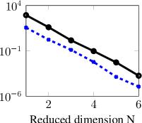
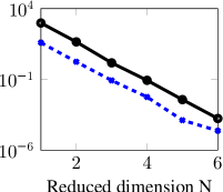
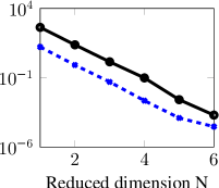
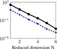
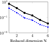
Figure 5: Comparison of maximal error estimator and
true error for the proteins in Table 2, respectively.

Figure 6 shows the error estimator and the true error of the finally constructed ROM over $\mu_{i}=\Xi$, for $i=1,...,11$ samples for each protein as in Table 2, respectively. It is evident that the error estimator for the final RB approximations of dimension $N=6$ is indeed an upper bound of the true error and a trend that both quantities behave similarly is clearly visible from the graphs. Consequently, the error estimators fall below the greedy tolerance of $10^{-3}$.

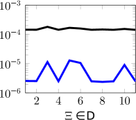
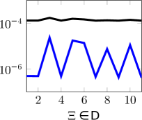
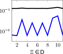
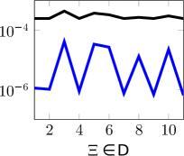
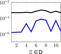
Figure 6: Comparison of error estimator and true error for
the final ROM for $\Xi\in D$ and for the proteins in Table 2,
respectively.

Figure 7 is used to validate the true error in Figure 6, whereby $20$ random values of the parameter domain $D$ which are different from those in the training set $\Xi$ are used. A common observation from these figures is that the true errors fall below $\mathcal{O}(10^{-4})$, which is an order of magnitude below the error estimator. The computational time taken to obtain the approximate solution $u_{N}(\mu)$ in the online phase is approximately $4.97\times 10^{-3}$ seconds on average, for any parameter $\mu\in D$.

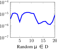
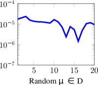
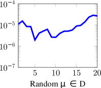
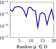
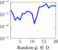
Figure 7: True error $\|u^{\mathcal{N}}(\mu)-u_{N}(\mu)\|_{2}$ for random parameters
$\mu\in D$ for the proteins in Table 2, respectively.

IV.4 Runtimes and Computational Speed-ups

Before we dive into the runtimes of the various phases of the RBM, we would like to make clear about some key notions of the two phases of the greedy algorithm, i.e., the offline and online phases, respectively. The offline phase is subdivided into two parts, the offline-offline phase, and the offline-online phase Hesthaven, Rozza, and Stamm (2016). The offline-offline phase involves computation of the snapshots and pre-computing the parameter-independent quantities. The offline-online phase involves computation of the error estimator and the RB approximation. On the other hand, the pure online phase is where the final ROM has been constructed after the accuracy of the reduced basis is fulfilled, and is independent of the greedy algorithm. In this phase, the ROM can be solved for any parameter value in the parameter domain, including those which are different from the training set.

Table 3 shows the runtimes and computational speed-ups obtained with the use of DEIM approximation during the offline-online phase of the RBM at a single iteration of the greedy algorithm and with the use of the RBM in solving the linear system. We use a modest PC with the following specifications: Intel (R) Core (TM)2 Duo CPU E8400 @ 3.00GHz with 8GB RAM. In this section, the PBE is applied to the protein fasciculin 1.

Runtime (seconds) and speed-up
	Without DEIM	With DEIM	Speed-up
Offline-online phase	96.29	4.84	20
Assemble and solve
ROM	8.36	9.91e-03	844

Table 3: Runtimes and speed-ups due to DEIM.

Table 4 shows the runtimes of computing the FOM and the ROM at a given parameter value, respectively. The runtimes at different phases of the RBM are also presented. Speed-up factors induced by solving the ROM are listed to visualize the big difference between the FOM and the ROM. The ROM is much faster and takes a split second to assemble and solve for any parameter value. In the offline phase of the RBM, which comprises the greedy algorithm, the dominating cost is that of solving the linear system of the FOM by AGMG (i.e., computing snapshot) at every iteration of the greedy algorithm. Miscellaneous in this case refers to the runtime to initialize the FDM, including assembling the FOM. The total RBM runtime includes the miscellaneous and offline runtimes.

Runtime (seconds) and speed-up
	FOM	ROM	Speed-up
Solve linear system	11.88	4.97e-03	7,616
Assemble and solve linear system	27.82	9.91e-03	5,500
Runtime (seconds) for RBM phases
Miscellaneous	Offline	Online	Total RBM
10.58	85.54	9.91e-03	96.12

Table 4: Runtimes and speed-ups for FOM, ROM and RBM.

Table 5 shows the runtimes of APBS and RBM for solving the FOM and the ROM at any given parameter value, respectively. The speed-up factor of RBM w.r.t. the APBS is also shown for different numbers of parameter values. It is evident that RBM is much more efficient than APBS when solving the system for many input parameter values (i.e. in a multi-query context). This is because we only need to solve a small system of order $N=6$ once the final ROM model has been constructed which takes approximately $9.91\times 10^{-3}$ seconds for each parameter value, whereas APBS solves the FOM besides the initial system setup.

In a nutshell, to solve the LPBE for any parameter value with APBS, it takes $22.893$ seconds, because the solver has to reconstruct the linear system. This implies that it takes approximately $2,289.3$ seconds to compute the potential for $100$ parameter values (neglecting the runtime to modify the input files). This is more expensive than the total RBM time of $96.12$ seconds. On the other hand, it takes the RBM approximately $9.91\times 10^{-1}$ seconds to solve the ROM of the LPBE for the same number of parameters values (i.e., 100).

The RBM only solves the FOM $N$ times during the expensive offline phase as stated in Algorithm 1. Moreover, the RBM utilizes the precomputed system matrices and vectors and only solves the ROM for the new parameter value, thus saving a significant amount of computational costs during the online phase. This efficient implementation of a new mathematical approach to solve the PBE holds great promise towards reducing computational costs in a multi-query scenario and molecular dynamics simulation.

Runtime (seconds) and speed-up for APBS and RBM
No. of parameters	APBS	RBM	Speed-up
1	22.893	$\approx 96.12$	0.24
10	228.93	$\approx 96.12$	2.38
100	2,289.3	$\approx 96.12$	24
1000	22,893	$\approx 106.12$	215.75

Table 5: Runtimes for APBS and RBM.

V Conclusions

In this paper, we have presented a new, computationally efficient approach to solving the PBE for varying parameter values. The RBM reduces the high-dimensional full order model by a factor of approximately $360,000$ and the computational time by a factor of approximately $7,600$. The error estimator provides fast convergence to the reduced basis approximation at an accuracy of $\mathcal{O}(10^{-3})$. The true error between the RBM and the FDM is smaller than $O(10^{-4})$, for all the parameter samples tested. DEIM provides a speed-up of 20 in the online phase by reducing the complexity of the nonaffine Dirichlet boundary conditions. This is achieved by only selecting a few entries from a high-dimensional vector which provides the most important information. Therefore, the RBM can be extremely beneficial in cases where simulations of the PBE for many input parameter values are required. This method can also be implemented in the available PBE solvers, for example, APBS, after a few adjustments regarding parametrization in the linear system are made. Our future research is based on two aspects. Firstly, we plan to develop a more efficient error estimator which is more rigorous than merely taking the norm of the residual. Secondly, we aim to develop a modified version of the LPBE which considers the PBE as interface problem by applying a range-separated tensor format. This is expected to reduce the computational complexity experienced by the current PBE studies, and to provide more accurate results due to the more realistic model.