Distributed Precoding Systems in Multi-Gateway Multibeam Satellites: Regularization and Coarse Beamforming

Abstract

This paper deals with the problem of beamforming design in a multibeam satellite, which is shared by different groups of terminals -clusters-, each served by an Earth station or gateway. Each gateway precodes the symbols addressed to its respective users; the design follows an MMSE criterion, and a regularization factor judiciously chosen allows to account for the presence of mutually interfering clusters, extending more classical results applicable to one centralized station. More importantly, channel statistics can be used instead of instantaneous channel state information, avoiding the exchange of information among gateways through backhaul links. The on-board satellite beamforming weights are designed to exploit the degrees of freedom of the satellite antennas to minimize the noise impact and the interference to some specific users. On-ground beamforming results are provided as a reference to compare the joint performance of MMSE precoders and on-board beamforming network. A non-adaptive design complements the results and makes them more amenable to practical use by designing a coarse beamforming network.

I Introduction

Relaying is a widespread mechanism to extend the coverage of wireless links by appropriate manipulation of the input signals, which might include amplification, filtering and beamforming, just to mention a few physical layer operations. Bent-pipe communication satellites can be considered as non-regenerative relays [1], essentially filtering and amplifying signals, although they are very complex communication systems and handle simultaneously many streams of information. The object of this study is a multibeam satellite which relays the signals coming from $M$ ground stations (gateways) to convey their communication with single-antenna terminals. The foot-print of a multibeam satellite is made of many spot-beams, hundreds in some specific commercial cases, which are synthesized by the on-board beamforming network (BFN) in combination with the antennas radiation pattern. Two implementation approaches are possible: single feed per beam and multiple feeds per beam. For the purpose of this paper, it is of specific interest the case of multiple feeds per beam, for which small subarrays are used for each spot-beam, and adjacent spot-beams share some of the array elements. This technology has some advantages since individual beams can overlap and a single reflector antenna served by several feeds can cover a larger area [1]. The on-board beamforming (OBBF) process contributes some flexibility to the shaping of the beams, although the configurability is in most cases quite limited, and real-time adaptation in the range of milliseconds is rarely feasible. Remarkably, a technology known as On-Ground Beamforming (OGBF) has emerged as an alternative solution for some specific cases, to avoid the need for a complex on-board digital processor. This technology has been used in some recent multibeam mobile satellite systems [2], and requires the exchange of all the feed signals between the satellite and the gateway, increasing the bandwidth demands on the feeder link due to the higher number of information streams.

Figure 1 depicts the conceptual abstraction of the multibeam satellite operation, with the following features to be highlighted: (i) the feeder links, from the gateways to the satellites, can be assumed transparent, whereas the user links are frequency non-selective; (ii) there is no interference between feeder links and user links, since the communication takes place on different frequency bands; (iii) a given cluster is made of several beams (see Figure 2), with one user per beam served at a time by a given frequency carrier; (iv) the user link frequency carriers are made available to all beams and clusters, in what it is known as full-frequency reuse.

One major challenge for multibeam satellites is the large spectral demand on the feeder link between the satellite and the operator stations, since it has to aggregate the traffic from all beams. Technology has contributed to a steady increase of this traffic during the last years due to, among other things, a more efficient reuse of spectrum across the different beams [3]. The use of different gateways can generate several parallel channels provided that the antennas guarantee the required spatial isolation, which is the case for frequencies in Ku-band or Ka-band. Thus, the different feeder links can reuse the whole available bandwidth.

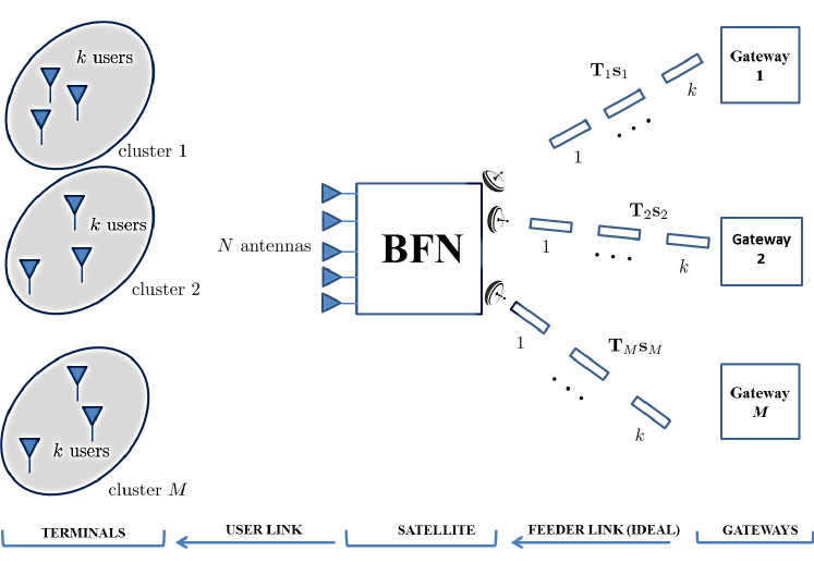
Figure 1: Satellite shared by a number of ground stations.

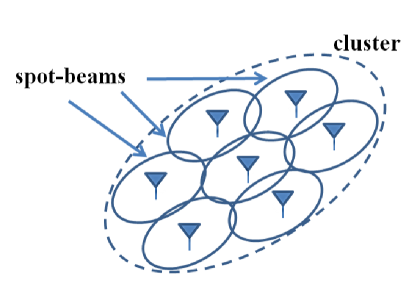
Figure 2: Cluster of beams.

The preprocessing of signals to communicate multiple-antennas in one-site with many users simultaneously is supported by theoretical bounds and practical schemes presented in many references. In the particular case of linear precoding, the seminal paper [4] analyzes the regularization of channel inversion at the transmitter to maximize the signal to interference and noise ratio (SINR), with specific focus on Rayleigh channels. On the other side, precoding for multibeam satellites has been extensively explored in the literature to fight interbeam interference in the case of a single gateway, see, e.g., [5] and [6] among others. Potential gain and calibration needs have been properly identified by these works. As opposed, results for multiple gateways are still incomplete; a centralized multi-gateway resource management, which for mathematical purposes can be assumed, is far from being realistic in practice [3], due to the backhaul links that would be needed to connect all the gateways. Some precoding schemes for multiple gateways without BFN are presented in [7], which assume the exchange of information for the design of their respective precoders. However, no integral approach conciliating the design of an on-board BFN and the use of several gateways, required to channelize the high throughput for an aggressive use of the user link spectrum, is known. The mapping of groups of beams to different gateways prevents from a centralized management, with inter-cluster interference more difficult to control.

In this work we try to keep the cooperation at a minimum, so that no information symbols are exchanged among the terrestrial gateways, each communicating with the terminals operating on its cluster. Initially each gateway is expected to know the channel state information (CSI) of the links originating from itself, including inter-cluster links, although the use of channel statistics is shown to predict quite conveniently the required information so the interaction among different clusters can be completely avoided. The global interplay of distributed precoders operating at the different gateways and the BFN on the satellite can be designed in such a way that different solutions accrue, each fitting the available information and flexibility of the involved subsystems. Specific regularization rules for the distributed precoders are obtained as an extension of the results for one cluster. As a reference, we compute the performance of the fully flexible OGBF with perfect CSI at both the gateways (CSIT) and receive terminals (CSIR). Starting from that, separate on-board BFN and precoders are derived. The performance indicator is the Mean Square Error (MSE) for three different settings: (i) intra-cluster interference driven; (ii) cancellation of interference leaked to specific off-cluster users; (iii) coarse fixed BFN designed as a trade-off solution. The latter scheme is particularly important, since it allows to fix the on-board BFN and confine the flexibility to the gateway precoders: some loss of performance is expected to achieve this more practical design.

After detailing the satellite relaying operation in Section II, we derive the optimal beamforming weights and gateway precoders, first for the OGBF case in Section III and then for separate on-board beamforming and ground precoders in Section IV. Both fixed and adaptive BFN weights are object of the study, with performance tested in the simulations shown before the conclusions.

Notation: Upper (lower) boldface letters denote matrices (vectors). $(.)^{H}$, $(.)^{T}$, $\operatorname{tr}\{\cdot\}$, $\mathbf{I}_{N}$, $\bm{0}$, $\text{diag}\{\cdot\}$ denote Hermitian transpose, transpose, matrix trace operator, $N\times N$ identity matrix, all-zero matrix, and diagonal matrix, respectively. $\mathbb{E}\left[{\cdot}\right]$ is the expected value operator.

II Satellite Relaying Operation

The satellite serves $K$ terminals at each channel use. All $K$ users get access to the same frequency spectrum, thus giving rise to both intra-cluster and inter-cluster interference. The satellite has $N$ radiation elements or feeds, with $N\geq K$. The $K\times 1$ vector comprising the values received by the $K$ users at a given time instant is written as

$${\mathbf{y}}=\widetilde{{\mathbf{H}}}\widetilde{{\mathbf{B}}}{\mathbf{x}}+{\mathbf{n}}$$ (1)

for $K\times 1$ vector ${\mathbf{x}}$ transmitted values and $K\times 1$ vector ${\mathbf{n}}$ zero-mean unit variance Additive White Gaussian Noise (AWGN), such that $\mathbb{E}\left[{{\mathbf{n}}{\mathbf{n}}^{H}}\right]=\mathbf{I}_{K}$. The BFN weights are included in matrix $\widetilde{{\mathbf{B}}}\in\mathbb{C}^{N\times K}$. $\widetilde{{\mathbf{H}}}\in\mathbb{C}^{K\times N}$ is the overall user link channel matrix whose element $[\widetilde{{\mathbf{H}}}]_{ij}$ represents the gain of the link between the $i$-th user and the $j$-th satellite feed.

As shown in Figure 1, the number of transmit ground stations is $M$, each sending $k$ signal streams simultaneously (in different frequency slots, for example) to the satellite, which makes use of $n$ antenna feeds to send those symbols to the $k$ users in the $m$th cluster, with $k\leq n\leq N$. The groups of $n$ feeds are not necessarily disjoint. The information transmitted from each ground station is written as ${\mathbf{x}}_{m}={\mathbf{T}}_{m}{\mathbf{s}}_{m}$, with ${\mathbf{T}}_{m}\in\mathbb{C}^{k\times k},m=1,\ldots,M$, a set of distributed precoding matrices, and ${\mathbf{s}}_{m}\in\mathbb{C}^{k\times 1},m=1,\ldots,M$ the symbols transmitted by the $m$th gateway. The initial model (1) can be detailed as

$${\mathbf{y}}=\widetilde{{\mathbf{H}}}\left[\begin{array}[]{ccc}\widetilde{{\mathbf{B}}}_{1}&\cdots&\widetilde{{\mathbf{B}}}_{M}\end{array}\right]\left[\begin{array}[]{c}{\mathbf{T}}_{1}{\mathbf{s}}_{1}\\ \vdots\\ {\mathbf{T}}_{M}{\mathbf{s}}_{M}\end{array}\right]+{\mathbf{n}}$$ (2)

where the tall matrices $\widetilde{{\mathbf{B}}}_{m}\in\mathbb{C}^{N\times k}$ contain the BFN weights assigned to gateway $m$, and $k\cdot M=K$. The input energy is normalized as $\mathbb{E}\left[{{\mathbf{s}}_{m}{\mathbf{s}}_{m}^{H}}\right]=\mathbf{I}_{k}$. The goal of the precoder at each transmitter is mainly the mitigation of the intra-cluster interference, while trying to reduce the negative impact of its interference on other clusters. The BFN should exploit the additional degrees of freedom to gain inter-cluster interference and/or noise resilience, preferably in a robust way against the uncertain location of the users.

More specifically, the notation can reflect that only a portion of feeds is involved per cluster. If $n$ denotes the number of feeds serving each cluster, the weights with content in the BFN can be collected by the tall submatrices ${\mathbf{B}}_{m}\in\mathbb{C}^{n\times k},m=1,\ldots,M$, with $k\leq n\leq N$. Each matrix $\widetilde{{\mathbf{B}}}_{m}$ in (2) only has $n$ non-zero rows, so we can write

$$\widetilde{{\mathbf{B}}}_{m}=\mathcal{S}_{m}{\mathbf{B}}_{m}$$ (3)

where $\mathcal{S}_{m}$ comprises $n$ columns of ${\mathbf{I}}_{N}$, in particular those with the indices of the feeds used by gateway $m$. With $n>k$, there are extra degrees of freedom to fight the inter-cluster interference and gain noise resilience without increasing the bandwidth of the user link. If we decompose the received signal and noise vectors in (1) into their respective vectors per cluster, ${\mathbf{y}}_{m}$ and ${\mathbf{n}}_{m}$, respectively, and ${\mathbf{H}}_{mp}$ is the channel between the $n$ feeds operated by the $p$th gateway and the $m$th cluster, then the initial signal model reads as

$$\begin{pmatrix}\mathbf{y}_{1}\\ \vdots\\ \mathbf{y}_{M}\end{pmatrix}=\underbrace{\begin{pmatrix}\mathbf{H}_{11}&\ldots&{\mathbf{H}}_{1M}\\ \vdots&\ddots&\vdots\\ {\mathbf{H}}_{M1}&\ldots&{\mathbf{H}}_{MM}\end{pmatrix}}_{{\mathbf{H}}}\begin{pmatrix}{\mathbf{B}}_{1}&&\\ &\ddots&\\ &&{\mathbf{B}}_{M}\end{pmatrix}\begin{pmatrix}{\mathbf{T}}_{1}{\mathbf{s}}_{1}\\ \vdots\\ {\mathbf{T}}_{M}{\mathbf{s}}_{M}\end{pmatrix}+\begin{pmatrix}\mathbf{n}_{1}\\ \vdots\\ \mathbf{n}_{M}\end{pmatrix}.$$ (4)

Note that, in this cluster-oriented notation, the channel matrix ${\mathbf{H}}\in\mathbb{C}^{K\times nM}$ does not coincide with $\widetilde{{\mathbf{H}}}$ in (2). If ${\mathbf{H}}$ is decomposed as $\left[\begin{array}[]{ccc}{\mathbf{H}}_{1}&\cdots&{\mathbf{H}}_{M}\end{array}\right]$, and since both expressions (4) and (2) need to be equivalent, we can readily conclude that ${\mathbf{H}}_{m}=\widetilde{{\mathbf{H}}}\mathcal{S}_{m}$.

The vector of samples received by users in cluster $m$ is decomposed as

$${\mathbf{y}}_{m}=\underbrace{{\mathbf{H}}_{mm}{\mathbf{B}}_{m}{\mathbf{T}}_{m}{\mathbf{s}}_{m}}_{\text{intra-cluster}}+\underbrace{\sum_{p\neq m}{\mathbf{H}}_{mp}{\mathbf{B}}_{p}{\mathbf{T}}_{p}{\mathbf{s}}_{p}}_{\text{inter-cluster}}+\underbrace{{\mathbf{n}}_{m}}_{\text{noise}}.$$ (5)

End users cannot cooperate, so that we consider a receiver of the form $\hat{\mathbf{s}}_{m}={\mathbf{D}}_{m}{\mathbf{y}}_{m}$, where the matrix ${\mathbf{D}}_{m}$ is $k\times k$ diagonal. The particular case in which the same scaling is used across the cluster will be also assumed later, with ${\mathbf{D}}_{m}=\frac{1}{\sqrt{t_{m}}}{\mathbf{I}}_{k}$.

As performance metric we use the aggregated MSE, or Sum MSE (SMSE), given by

$$\mathop{\rm SMSE}=\sum_{m=1}^{M}\operatorname{tr}\left\{{\mathbf{E}}_{m}\right\},$$ (6)

with

$${\mathbf{E}}_{m}\triangleq\mathbb{E}\left[{({\mathbf{s}}_{m}-\hat{\mathbf{s}}_{m})({\mathbf{s}}_{m}-\hat{\mathbf{s}}_{m})^{H}}\right].$$ (7)

The expectation is computed with respect to the symbols and the noise for a fixed channel, and reads as

$$\mathop{\rm SMSE}=\sum_{m=1}^{M}\operatorname{tr}\left\{{\mathbf{I}}_{k}-{\mathbf{D}}_{m}{\mathbf{H}}_{mm}{\mathbf{B}}_{m}{\mathbf{T}}_{m}-{\mathbf{T}}_{m}^{H}{\mathbf{B}}_{m}^{H}{\mathbf{H}}_{mm}^{H}{\mathbf{D}}_{m}^{H}\right.+\\ \left.{\mathbf{T}}_{m}^{H}{\mathbf{B}}_{m}^{H}\left(\sum_{p=1}^{M}{\mathbf{H}}_{pm}^{H}{\mathbf{D}}_{p}^{H}{\mathbf{D}}_{p}{\mathbf{H}}_{pm}\right){\mathbf{B}}_{m}{\mathbf{T}}_{m}+{\mathbf{D}}_{m}{\mathbf{D}}_{m}^{H}\right\},$$ (8)

written in such a way that the impact of ${\mathbf{T}}_{m}$ and ${\mathbf{B}}_{m}$ on the overall error is limited to the $m$th term of the summation. This way of dealing together with the interference posed on the same cluster and leaked to other clusters have been explored in other works such as [8], where the Signal to Leakage and Noise Ratio (SLNR) was maximized for a single transmitter. Even further, [9] showed that the minimization of the MSE and the maximization of SLNR lead to equivalent solutions for equal allocation of power for all users, a single base station and single user terminals. It is important to remark that the minimization of SMSE and the maximization of sum capacity are related, although they can suffer from lack of fairness issues with less favored users [10].

For convenience, we define

$${\mathbf{A}}_{m}\triangleq\sum_{p=1}^{M}{\mathbf{H}}_{pm}^{H}{\mathbf{D}}_{p}^{H}{\mathbf{D}}_{p}{\mathbf{H}}_{pm}\in\mathbb{C}^{n\times n},\qquad{\mathbf{X}}_{m}\triangleq{\mathbf{H}}_{mm}^{H}{\mathbf{D}}_{m}^{H}\in\mathbb{C}^{n\times k},$$ (9)

so that

$$\mathop{\rm SMSE}=\sum_{m=1}^{M}\operatorname{tr}\{{\mathbf{I}}_{k}-{\mathbf{X}}_{m}^{H}{\mathbf{B}}_{m}{\mathbf{T}}_{m}-{\mathbf{T}}_{m}^{H}{\mathbf{B}}_{m}^{H}{\mathbf{X}}_{m}+{\mathbf{T}}_{m}^{H}{\mathbf{B}}_{m}^{H}{\mathbf{A}}_{m}{\mathbf{B}}_{m}{\mathbf{T}}_{m}+{\mathbf{D}}_{m}{\mathbf{D}}_{m}^{H}\}.$$ (10)

The SMSE in (8), or alternatively (10), is the starting point to explore several solutions for the precoding matrices $\{{\mathbf{T}}_{m}\}_{m=1}^{M}$ and BFN weights $\{{\mathbf{B}}_{m}\}_{m=1}^{M}$, each targetting different constraints. Under the proposed global MSE framework, all the involved coefficients in the transmission process would be the result of minimizing the overall MSE:

$$\text{(P1)}\qquad\{{\mathbf{T}}_{m},{\mathbf{B}}_{m},{\mathbf{D}}_{m}\}_{m=1}^{M}=\arg\min\sum_{m=1}^{M}\operatorname{tr}\{{\mathbf{E}}_{m}\}\qquad\text{s. to }\operatorname{tr}\{{\mathbf{B}}_{m}{\mathbf{T}}_{m}{\mathbf{T}}_{m}^{H}{\mathbf{B}}_{m}^{H}\}\leq P_{m},$$ (11)

with $P_{m}$ the power allocated to the $m$-th cluster. This is the power limit for each group of $n$ antenna feeds; note that we are not considering per-feed-constraints at the satellite, left for future studies. The overall available power on the satellite is $P=\sum_{m=1}^{M}P_{m}$.

We are interested in addressing the separate optimization of $\{{\mathbf{T}}_{m}\}_{m=1}^{M}$ and $\{{\mathbf{B}}_{m}\}_{m=1}^{M}$, since the flexibility and amount of CSI is not necessarily the same on-board the satellite and on-ground. Only for the OGBF case, with all weights operated at the gateways, a joint $\{{\mathbf{B}}_{m}{\mathbf{T}}_{m}\}_{m=1}^{M}$ matrix is considered.

No closed-form seems to be available for variables $\{{\mathbf{D}}_{m},{\mathbf{T}}_{m},{\mathbf{B}}_{m}\}_{m=1}^{M}$ minimizing the SMSE in (11) under transmit power constraints, so a multistage approach is explored. Initially we will assume that perfect knowledge is available to obtain the optimum weights, with practical constraints being imposed later to come up with a fixed BFN and no exchange of signalling information among gateways.

III On-Ground Beamforming

For setting a reference we start with the most favorable case, for which CSIT is perfectly known and all coefficients can be correspondingly adjusted. Joint adaptation of precoding and beamforming coefficients can be applied if their combined operation takes place at the ground stations, by using the OGBF technology detailed in the Introduction. All coefficients can be directly manipulated on the ground, at the price of a higher number of exchanged signals with the satellite, one per feed managed by the corresponding gateway.

The grouping of ${\mathbf{B}}_{m}$ and ${\mathbf{T}}_{m}$ in (8) leads us to write ${\mathbf{F}}_{m}\triangleq{\mathbf{B}}_{m}{\mathbf{T}}_{m}$, and optimize directly with respect to these ${\mathbf{F}}_{m}$ matrices. Since no closed-form solution seems to be available, we optimize cyclically with respect to $\{{\mathbf{F}}_{m}\}_{m=1}^{M}$ keeping $\{{\mathbf{D}}_{m}\}_{m=1}^{M}$ fixed, and then with respect to $\{{\mathbf{D}}_{m}\}_{m=1}^{M}$ keeping $\{{\mathbf{F}}_{m}\}_{m=1}^{M}$ fixed. In this way, convergence in the cost is guaranteed [11]. With fixed $\{{\mathbf{D}}_{m}\}_{m=1}^{M}$, the optimization decouples into $M$ separate problems, for $m=1,\ldots,M$:

$$\text{(P2)}\quad{\mathbf{F}}_{m}=\arg\min\operatorname{tr}\{{\mathbf{I}}_{k}-{\mathbf{X}}_{m}^{H}{\mathbf{F}}_{m}-{\mathbf{F}}_{m}^{H}{\mathbf{X}}_{m}+{\mathbf{F}}_{m}^{H}{\mathbf{A}}_{m}{\mathbf{F}}_{m}+{\mathbf{D}}_{m}{\mathbf{D}}_{m}^{H}\}\quad\text{s. to }\operatorname{tr}\{{\mathbf{F}}_{m}{\mathbf{F}}_{m}^{H}\}\leq P_{m}.$$ (12)

The minimization of (12) reduces to a Least Squares problem with a quadratic inequality constraint. The solution is found as follows, for $m=1,\ldots,M$ and $M>1$:

• First, check whether the unconstrained solution ${\mathbf{F}}_{m}={\mathbf{A}}_{m}^{-1}{\mathbf{X}}_{m}$ is feasible; if so, stop.

• Otherwise, the constraint is satisfied with equality; the solution is ${\mathbf{F}}_{m}=({\mathbf{A}}_{m}+\nu_{m}{\mathbf{I}}_{n})^{-1}{\mathbf{X}}_{m}$, where the Lagrange multiplier $\nu_{m}$ has to be numerically computed to meet the power constraint $\operatorname{tr}\{{\mathbf{F}}_{m}{\mathbf{F}}_{m}^{H}\}=P_{m}$, see the Appendix.

Now we fix the matrices $\{{\mathbf{F}}_{m}\}_{m=1}^{M}$ and need to find $\{{\mathbf{D}}_{m}\}_{m=1}^{M}$. We rewrite the SMSE (8) as

$$\mathop{\rm SMSE}=\sum_{m=1}^{M}\operatorname{tr}\left\{{\mathbf{I}}_{k}-{\mathbf{D}}_{m}{\mathbf{H}}_{mm}{\mathbf{F}}_{m}-{\mathbf{F}}_{m}^{H}{\mathbf{H}}_{mm}^{H}{\mathbf{D}}_{m}^{H}\right.+\\ \left.{\mathbf{D}}_{m}\left(\sum_{p=1}^{M}{\mathbf{H}}_{mp}{\mathbf{F}}_{p}{\mathbf{F}}_{p}^{H}{\mathbf{H}}_{mp}^{H}\right){\mathbf{D}}_{m}^{H}+{\mathbf{D}}_{m}{\mathbf{D}}_{m}^{H}\right\}$$ (13)

and define

$${\mathbf{C}}_{m}\triangleq{\mathbf{I}}_{k}+\sum_{p=1}^{M}{\mathbf{H}}_{mp}{\mathbf{F}}_{p}{\mathbf{F}}_{p}^{H}{\mathbf{H}}_{mp}^{H}\in\mathbb{C}^{k\times k},\qquad{\mathbf{G}}_{m}\triangleq{\mathbf{F}}_{m}^{H}{\mathbf{H}}_{mm}^{H}\in\mathbb{C}^{k\times k},$$ (14)

so that we obtain the following compact expression for the SMSE:

$$\mathop{\rm SMSE}=\sum_{m=1}^{M}\operatorname{tr}\{{\mathbf{I}}_{k}-{\mathbf{D}}_{m}{\mathbf{G}}_{m}^{H}-{\mathbf{G}}_{m}{\mathbf{D}}_{m}^{H}+{\mathbf{D}}_{m}{\mathbf{C}}_{m}{\mathbf{D}}_{m}^{H}\}.$$ (15)

The minimization of (15) subject to ${\mathbf{D}}_{m}$ being diagonal is straightforward: if we let ${\mathbf{D}}_{m}=\text{diag}\{\begin{array}[]{ccc}d_{1}^{(m)}&\cdots&d_{k}^{(m)}\end{array}\}$, then

$$d_{j}^{(m)}=\frac{[{\mathbf{G}}_{m}]_{jj}}{[{\mathbf{C}}_{m}]_{jj}},\qquad j=1,\ldots,k,\quad m=1,\ldots,M.$$ (16)

The single gateway case ($M=1$) offers the best possible performance since all streams can have access to all feeds, achieving a better attenuation of the co-channel interference. In the above computations it must be noted that ${\mathbf{A}}_{m}$ is no longer full-rank; from (9), we have that the rank of ${\mathbf{A}}_{m}$ is not higher than $K$. The unconstrained solution which must be tested first for feasibility is ${\mathbf{F}}={\mathbf{A}}^{\dagger}{\mathbf{X}}$, with ${\mathbf{A}}^{\dagger}$ the pseudo-inverse of ${\mathbf{A}}$, and subscript $m$ dropped. Even further, if the scaling parameter is the same for all terminals, with ${\mathbf{D}}=(1/\sqrt{t}){\mathbf{I}}_{K}$, then the previous mathematical derivations can be simplified. Thus, ${\mathbf{F}}$ in (12) is simply given by

$${\mathbf{F}}=\sqrt{t}({\mathbf{H}}^{H}{\mathbf{H}}+\gamma{\mathbf{I}}_{K}){\mathbf{H}}^{H}$$ (17)

and $\gamma=K/P$. This result is already reported in [5], and can be proved by using the eigen-value decomposition of the channel Gramian ${\mathbf{H}}^{H}{\mathbf{H}}={\mathbf{U}}{\mathbf{S}}{\mathbf{U}}^{H}$ and similar steps to those exposed in the next section.

IV On-Board Beamforming

On-board beamforming needs only the exchange of one stream per user, not per feed, and it is the most common in practice, with different degrees of flexibility. Fully adaptive OBBF weights turn out to be highly challenging from the implementation point of view and, as a general rule, the adaptation time scale of BFN weights is more constrained than that of ground precoding weights [2]. This is why we split the adaptation of both sets of coefficients in this section, in an effort to leverage their separate roles and eventually design a fixed BFN or with a limited degree of programmability.

The complexity of (P1) is such that no closed-form expressions can be jointly obtained. For convenience, we assume that the beamforming matrices are semi-unitary, with orthonormal columns:

$${\mathbf{B}}_{m}^{H}{\mathbf{B}}_{m}={\mathbf{I}}_{k},m=1,\ldots,M.$$ (18)

Any rank-$k$ ${\mathbf{B}}_{m}\in\mathbb{C}^{n\times k}$ can be non-uniquely factorized as ${\mathbf{B}}_{m}={\mathbf{B}}_{m}^{0}{\mathbf{R}}$, with invertible ${\mathbf{R}}\in\mathbb{C}^{k\times k}$ and ${\mathbf{B}}_{m}^{0}\in\mathbb{C}^{n\times k}$ with orthonormal columns. As beamforming weights we choose ${\mathbf{B}}_{m}^{0}$, and ${\mathbf{R}}$ can be embedded in the precoder ${\mathbf{T}}$ without affecting the minimum MSE. With this, the power constraint in (P1) can be written as $\operatorname{tr}\{{\mathbf{T}}_{m}{\mathbf{T}}_{m}^{H}\}\leq P_{m}$.
If we fix the beamforming weights, then the solution of the previous section applies, by using ${\mathbf{B}}_{m}^{H}{\mathbf{A}}_{m}{\mathbf{B}}_{m}$ and ${\mathbf{B}}_{m}^{H}{\mathbf{X}}_{m}$ in lieu of ${\mathbf{A}}_{m}$ and ${\mathbf{X}}_{m}$, respectively:

$${\mathbf{T}}_{m}=\left({\mathbf{B}}_{m}^{H}{\mathbf{A}}_{m}{\mathbf{B}}_{m}+\nu_{m}{\mathbf{I}}_{k}\right)^{-1}{\mathbf{B}}_{m}^{H}{\mathbf{H}}_{mm}^{H}{\mathbf{D}}_{m}^{H}.$$ (19)

Some of the Lagrange multipliers $\{\nu_{m}\}_{m=1}^{M}$ could be zero if the power constraint of the $m$-th cluster is not active. Note that the different scaling matrices $\{{\mathbf{D}}_{m}\}_{m=1}^{M}$ are also embedded in $\bm{{\mathbf{A}}}_{m}$ as per (9). Again, an iterative process could serve to iterate till convergence $\{{\mathbf{T}}_{m}\}_{m=1}^{M}$ and $\{{\mathbf{D}}_{m}\}_{m=1}^{M}$. In the particular case in which ${\mathbf{D}}_{m}=\frac{1}{\sqrt{t_{m}}}{\mathbf{I}}_{k}$, i.e., the same scalar applies for all users belonging to the same cluster, then ${\mathbf{T}}_{m}$ is written as

$${\mathbf{T}}_{m}=\sqrt{t_{m}}\left({\mathbf{B}}_{m}^{H}(t_{m}{\mathbf{A}}_{m}){\mathbf{B}}_{m}+\nu_{m}^{\prime}{\mathbf{I}}_{k}\right)^{-1}{\mathbf{B}}_{m}^{H}{\mathbf{H}}_{mm}^{H}$$ (20)

where $\nu_{m}^{\prime}=t_{m}\nu_{m}$. ${\mathbf{A}}_{m}$, the sum of the channel Gramians from those feeds managed by the $m$th gateway to users in all clusters, can be expressed, from (9), as

$${\mathbf{A}}_{m}=(1/t_{m})({\mathbf{H}}_{mm}^{H}{\mathbf{H}}_{mm}+\bm{\Sigma}_{m})$$ (21)

with

$$\bm{\Sigma}_{m}\triangleq\sum_{\begin{subarray}{c}p=1\\ p\neq m\end{subarray}}^{M}\frac{t_{m}}{t_{p}}{\mathbf{H}}_{pm}^{H}{\mathbf{H}}_{pm}.$$ (22)

The first term in ${\mathbf{A}}_{m}$ corresponds to the intra-cluster channel, whereas the second collects the leakage channel to all other clusters. For practical reasons, the acquisition of the inter-cluster channels to make $\bm{\Sigma}_{m}$ available to gateway $m$ is difficult to guarantee in practice. Even in the case that ${\mathbf{H}}_{pm}$ were known, the scaling parameters $\{t_{m}\}$ present in $\bm{\Sigma}_{m}$ would need coordination for their computation; a sequential process, for instance, would obtain $\{\nu_{m}^{\prime}\}$ for an initial set of $\{t_{m}\}$, set which would be recomputed for the obtained values of $\{\nu_{m}^{\prime}\}$, and so on. Message passing algorithms such as in [12] could be devised for this process, although are left outside the scope of this paper, which hinges on the autonomous operation of the gateways. To the end of simplifying the implementation, we will consider that ${\mathbf{B}}_{m}^{H}\bm{\Sigma}_{m}{\mathbf{B}}_{m}$ is approximated by $c_{m}\cdot{\mathbf{I}}_{K}$, with $c_{m}$ a constant which can be absorbed by the regularization factor. Thus, by reducing ${\mathbf{B}}_{m}^{H}(t_{m}{\mathbf{A}}_{m}){\mathbf{B}}_{m}$ to ${\mathbf{B}}_{m}^{H}{\mathbf{H}}_{mm}^{H}{\mathbf{H}}_{mm}{\mathbf{B}}_{m}+c_{m}{\mathbf{I}}_{k}$, the precoder of the $m$th gateway is

$${\mathbf{T}}_{m}=\sqrt{t_{m}}\left({\mathbf{B}}_{m}^{H}{\mathbf{H}}_{mm}^{H}{\mathbf{H}}_{mm}{\mathbf{B}}_{m}+\gamma_{m}{\mathbf{I}}_{k}\right)^{-1}{\mathbf{B}}_{m}^{H}{\mathbf{H}}_{mm}^{H},$$ (23)

with $\gamma_{m}=\nu_{m}^{\prime}+c_{m}$. The regularization factors $\gamma_{m}$ need to be obtained so that the contribution of the $m$-th gateway to the SMSE is minimized, as addressed in the following sections. If $\gamma_{m}=k/P_{m}$, this is the intra-cluster MMSE precoder [5]. Note that the structure of the precoder is the same as that obtained from considering $\bm{\Sigma}_{m}={\mathbf{0}}$. A variant which operates with the full ${\mathbf{A}}_{m}$ matrix in (21) is presented in [13], and it is left out of the scope of this work.

As stated eariler, we need to point out that the separated optimization of the ground precoders $\{{\mathbf{T}}_{m}\}_{m=1}^{M}$ and the BFN $\{{\mathbf{B}}_{m}\}_{m=1}^{M}$ has as ultimate goal to fix the BFN and let the precoders adapt to the channel variations. This is why we do not pursue the full optimization of ${\mathbf{B}}_{m}$ in (P1) for fixed ${\mathbf{T}}_{m}$ and enter into a sequential minimization process as that in Section III, but instead try to decouple the derivation of ${\mathbf{B}}_{m}$ from ${\mathbf{T}}_{m}$. Next we illustrate how to obtain the scaling $t_{m}$ and the regularization factor $\gamma_{m}$ in (23) under different restrictions on ${\mathbf{B}}_{m}$.

IV-A Pre-fixed BFN

If the $\{{\mathbf{B}}_{m}\}$ weights are already in-place and cannot be altered, then the parameters to optimize are $\{t_{m},\gamma_{m}\}$ in (23). The problem can be posed as

$$\text{(P3)}\qquad\{t_{m},\gamma_{m}\}_{m=1}^{M}=\arg\min\operatorname{tr}\{{\mathbf{E}}_{m}\}\qquad\text{s. to }\operatorname{tr}\{{\mathbf{T}}_{m}{\mathbf{T}}_{m}^{H}\}\leq P_{m}.$$ (24)

This error is written as

$$\operatorname{tr}\{{\mathbf{E}}_{m}\}=\operatorname{tr}\{{\mathbf{I}}_{k}\}-2\operatorname{tr}\{({\mathbf{B}}_{m}^{H}{\mathbf{H}}_{mm}^{H}{\mathbf{H}}_{mm}{\mathbf{B}}_{m}+\gamma_{m}{\mathbf{I}}_{k})^{-1}{\mathbf{B}}_{m}^{H}{\mathbf{H}}_{mm}^{H}{\mathbf{H}}_{mm}{\mathbf{B}}_{m}\}\\ +\operatorname{tr}\{({\mathbf{B}}_{m}^{H}{\mathbf{H}}_{mm}^{H}{\mathbf{H}}_{mm}{\mathbf{B}}_{m}+\gamma_{m}{\mathbf{I}}_{k})^{-1}{\mathbf{B}}_{m}^{H}({\mathbf{H}}_{mm}^{H}{\mathbf{H}}_{mm}+\bm{\Sigma}_{m}){\mathbf{B}}_{m}({\mathbf{B}}_{m}^{H}{\mathbf{H}}_{mm}^{H}{\mathbf{H}}_{mm}{\mathbf{B}}_{m}+\gamma_{m}{\mathbf{I}}_{k})^{-1}\cdot\\ {\mathbf{B}}_{m}^{H}{\mathbf{H}}_{mm}^{H}{\mathbf{H}}_{mm}{\mathbf{B}}_{m}\}+\operatorname{tr}\left\{\frac{1}{t_{m}}{\mathbf{I}}_{k}\right\}.$$ (25)

Note that all $M$ minimization problems in (P3) are coupled through the inter-cluster term $\bm{\Sigma}_{m}$. They can be decoupled if we assume that all $\{t_{m}\}$ are similar, so that message exchange among the gateways can be avoided during the optimization phase:

$$\bm{\Sigma}_{m}\approx\sum_{\begin{subarray}{c}p=1\\ p\neq m\end{subarray}}^{M}{\mathbf{H}}_{pm}^{H}{\mathbf{H}}_{pm}.$$ (26)

This looks like a reasonable assumption for large numbers of users, as the results in Section V will show. As a consequence, the power restrictions in (24) become active, with $t_{m}$ taking the highest possible value.

With the $M$ problems decoupled, the regularization factor $\gamma_{m}$ at each gateway precoder (23) can be designed so that the contribution $\operatorname{tr}\{{\mathbf{E}}_{m}\}$ to the SMSE is minimized. If this can be effectively applied, then the resulting precoder will be inter-cluster aware. The optimum value is given by the following lemma, which is proved in the Appendix.

Lemma 1

If we write the eigen-decomposition

$${\mathbf{B}}_{m}^{H}{\mathbf{H}}_{mm}^{H}{\mathbf{H}}_{mm}{\mathbf{B}}_{m}={\mathbf{U}}_{m}{\mathbf{S}}_{m}{\mathbf{U}}_{m}^{H}$$ (27)

with ${\mathbf{S}}_{m}=\text{diag}\{\begin{array}[]{ccc}\lambda_{1}^{(m)}&\cdots&\lambda_{k}^{(m)}\end{array}\}$, then the regularization factor $\gamma_{m}$ minimizing $\operatorname{tr}\{{\mathbf{E}}_{m}\}$ is the solution of the following equation:

$$\sum_{i=1}^{k}\frac{\lambda_{i}^{(m)}}{(\lambda_{i}^{(m)}+\gamma_{m})^{3}}\left(\gamma_{m}-\sigma_{ii}^{(m)}-\frac{k}{P_{m}}\right)=0$$ (28)

with $\sigma_{ii}^{(m)}$ the $i$th diagonal entry of ${\mathbf{U}}_{m}^{H}{\mathbf{B}}_{m}^{H}\bm{\Sigma}_{m}{\mathbf{B}}_{m}{\mathbf{U}}_{m}$. The corresponding scaling parameter of the precoder and receiver is given by

$$t_{m}=P_{m}/\sum_{i=1}^{k}\frac{\lambda_{i}^{(m)}}{(\lambda_{i}^{(m)}+\gamma_{m})^{2}}.$$ (29)

If all $\sigma_{ii}^{(m)}$ are equal to zero -no inter-cluster interference- then the solution to (28) is trivially seen to be $\gamma_{m}=k/P_{m}$, similarly to [4]. More generally, it can be readily seen to lie in the interval $[k/P_{m},k/P_{m}+\max(\sigma_{ii}^{(m)})]$. However, its derivation relies on the knowledge of $\bm{\Sigma}_{m}$, which participates in (28) through $\sigma_{ii}^{(m)}$. Even though we use the approximation in (26), the lack of coordination among gateways prevents the acquisition of the channel response from feeds serving cluster $m$ to terminals in all other clusters; we propose instead to make use of the expected leakage channel Gramians, thus avoiding their instantaneous acquisition. With this, we approximate (22) as

$$\bm{\Sigma}_{m}\approx\hat{\bm{\Sigma}}_{m}=\sum_{\begin{subarray}{c}p=1\\ p\neq m\end{subarray}}^{M}\mathbb{E}\left[{{\mathbf{H}}_{pm}^{H}{\mathbf{H}}_{pm}}\right].$$ (30)

In addition to the numerical solution of (28), we will also test in the simulations the following approximation:

$$\gamma_{m}=k/P_{m}+\operatorname{tr}\{{\mathbf{B}}_{m}^{H}\hat{\bm{\Sigma}}_{m}{\mathbf{B}}_{m}\}/k.$$ (31)

The first term $k/P_{m}$ is the regularization factor for intra-cluster precoders; the second term comes from approximating ${\mathbf{B}}_{m}^{H}\bm{\Sigma}_{m}{\mathbf{B}}_{m}$ by $c_{m}{\mathbf{I}}_{k}$ in (23), in such a way that the trace of both matrices is the same (for identical $\{t_{m}\}$ values in $\bm{\Sigma}_{m}$). The precoder computed in this way is still inter-cluster aware, yielding an edge with respect to intra-cluster precoders. We will show the validity of this approach in the simulations.

IV-B Adaptive BFN

If the BFN weights can be optimized, at first sight we should choose ${\mathbf{B}}_{m}$ under the SMSE criterion to minimize the error term $\operatorname{tr}\{{\mathbf{E}}_{m}\}$ in (P1) as

$$\text{(P4)}\quad\{{\mathbf{B}}_{m}\}_{m=1}^{M} =\arg\min\operatorname{tr}\{{\mathbf{I}}_{k}-\frac{1}{\sqrt{t_{m}}}\left({\mathbf{H}}_{mm}{\mathbf{B}}_{m}{\mathbf{T}}_{m}-{\mathbf{T}}_{m}^{H}{\mathbf{B}}_{m}^{H}{\mathbf{H}}_{mm}^{H}\right)+{\mathbf{T}}_{m}^{H}{\mathbf{B}}_{m}^{H}{\mathbf{A}}_{m}{\mathbf{B}}_{m}{\mathbf{T}}_{m}+\frac{1}{t_{m}}{\mathbf{I}}_{k}\}$$ (32)

$$\text{s. to}\quad{\mathbf{B}}_{m}^{H}{\mathbf{B}}_{m}={\mathbf{I}}_{k}.$$

Desirably, we would like to decouple the derivation of BFN ${\mathbf{B}}_{m}$ and the precoder ${\mathbf{T}}_{m}$ as much as possible to simplify the practical implementation, so that different degrees of flexibility can be accommodated. No closed-form seems to be feasible for ${\mathbf{B}}_{m}$ minimizing all three components together. For the zero-forcing version of the precoder ${\mathbf{T}}_{m}$, that is, with $\gamma_{m}=0$ in (23), the inter-cluster contribution in (P4) becomes independent of ${\mathbf{B}}_{m}$, and only remain the inter-cluster interference and additive noise components. If ${\mathbf{B}}_{m}$ is designed to minimize the effect of the latter, then $t_{m}$ in (P4) needs to be maximized. This problem is written now as

$$\text{(P5)}\quad\{{\mathbf{B}}_{m},t_{m}\}_{m=1}^{M} = \arg\min\operatorname{tr}\left\{\frac{1}{t_{m}}{\mathbf{I}}_{k}\right\}$$ (33)

s. to $$\quad\left\{\begin{array}[]{ll}{\mathbf{B}}_{m}^{H}{\mathbf{B}}_{m}={\mathbf{I}}_{k},\\ \operatorname{tr}\{{\mathbf{T}}_{m}{\mathbf{T}}_{m}^{H}\}\leq P_{m}\end{array}\right.$$ (36)

with ${\mathbf{T}}_{m}=\sqrt{t_{m}}({\mathbf{B}}_{m}^{H}{\mathbf{H}}_{mm}^{H}{\mathbf{H}}_{mm}{\mathbf{B}}_{m})^{-1}{\mathbf{B}}_{m}^{H}{\mathbf{H}}_{mm}^{H}$. It can be readily seen that, at the optimum point, the power constraint must hold with equality, and

$$t_{m}=P_{m}/\operatorname{tr}\{{\mathbf{T}}_{m}{\mathbf{T}}_{m}^{H}\}=P_{m}/\operatorname{tr}\{({\mathbf{B}}_{m}^{H}{\mathbf{H}}_{mm}^{H}{\mathbf{H}}_{mm}{\mathbf{B}}_{m})^{-1}\}.$$ (37)

This design scheme effectively decouples the derivation of BFN and precoder, and exploits the degrees of freedom available at the satellite to increase the resilience against the noise. As a remark, the inter-cluster leakage will be again addressed by the proper design of the regularization factor as shown later. As noted in the previous paragraph for fixed ${\mathbf{B}}_{m}$, the regularization factor $\gamma_{m}$ in (23) has a non-trivial dependence on the channel and the BFN.

Let us write the eigenvalue decomposition

$${\mathbf{H}}_{mm}^{H}{\mathbf{H}}_{mm}={\mathbf{U}}_{H,m}\left(\begin{array}[]{cc}{\mathbf{S}}_{H,m}&{\mathbf{0}}\\ {\mathbf{0}}&{\mathbf{0}}\end{array}\right){\mathbf{U}}_{H,m}^{H},$$ (38)

with ${\mathbf{S}}_{H,m}=\text{diag}\{\begin{array}[]{ccc}\lambda_{1}^{(m)}&\cdots&\lambda_{k}^{(m)}\end{array}\}$, and $\lambda_{i}^{(m)}$ denoting the $k$ non-zero eigenvalues of ${\mathbf{H}}_{mm}^{H}{\mathbf{H}}_{mm}$ in decreasing order. With this, we have

$$\operatorname{tr}\{({\mathbf{B}}_{m}^{H}{\mathbf{H}}_{mm}^{H}{\mathbf{H}}_{mm}{\mathbf{B}}_{m})^{-1}\}=\sum_{i=1}^{k}\frac{1}{\lambda_{i}({\mathbf{B}}_{m}^{H}{\mathbf{U}}_{H,m}{\tiny\left(\begin{array}[]{cc}{\mathbf{S}}_{H,m}&{\mathbf{0}}\\ {\mathbf{0}}&{\mathbf{0}}\end{array}\right)}{\mathbf{U}}_{H,m}^{H}{\mathbf{B}}_{m})}$$ (39)

with $\lambda_{i}({\mathbf{Z}}),i=1,\ldots,k$, denoting the eigenvalues of ${\mathbf{Z}}$ in decreasing order. ${\mathbf{U}}_{H,m}^{H}{\mathbf{B}}_{m}$ has orthonormal columns, since ${\mathbf{B}}_{m}^{H}{\mathbf{B}}_{m}={\mathbf{I}}_{k}$, so we can apply Poincaré separation theorem [14], which bounds the eigenvalues of ${\mathbf{B}}_{m}^{H}{\mathbf{U}}_{H,m}{\tiny\left(\begin{array}[]{cc}{\mathbf{S}}_{H,m}&{\mathbf{0}}\\ {\mathbf{0}}&{\mathbf{0}}\end{array}\right)}{\mathbf{U}}_{H,m}^{H}{\mathbf{B}}_{m}$ in terms of those of ${\tiny\left(\begin{array}[]{cc}{\mathbf{S}}_{H,m}&{\mathbf{0}}\\ {\mathbf{0}}&{\mathbf{0}}\end{array}\right)}$ in the following way:

$$\lambda_{i}^{(m)}\geq\lambda_{i}({\mathbf{B}}_{m}^{H}{\mathbf{U}}_{H,m}{\tiny\left(\begin{array}[]{cc}{\mathbf{S}}_{H,m}&{\mathbf{0}}\\ {\mathbf{0}}&{\mathbf{0}}\end{array}\right)}{\mathbf{U}}_{H,m}^{H}{\mathbf{B}}_{m})\geq\lambda_{n-k+i}^{(m)}$$ (40)

so that

$$\sum_{i=1}^{k}\frac{1}{\lambda_{i}({\mathbf{B}}_{m}^{H}{\mathbf{U}}_{H,m}{\tiny\left(\begin{array}[]{cc}{\mathbf{S}}_{H,m}&{\mathbf{0}}\\ {\mathbf{0}}&{\mathbf{0}}\end{array}\right)}{\mathbf{U}}_{H,m}^{H}{\mathbf{B}}_{m})}\geq\sum_{i=1}^{k}\frac{1}{\lambda_{i}^{(m)}}.$$ (41)

The lower bound is achieved for ${\mathbf{B}}_{m}^{H}{\mathbf{U}}_{H,m}=[\begin{array}[]{cc}{\mathbf{I}}_{k}&{\mathbf{0}}\end{array}]$, so the optimal solution ${\mathbf{B}}_{m}$ must be equal to the first $k$ columns of ${\mathbf{U}}_{H,m}$. With this solution the $n-k$ degrees of freedom provided by ${\mathbf{B}}_{m}$ are exploited to reduce the impact of noise enhancement due to the intra-cluster cancellation.

The design of the BFN is such that ${\mathbf{B}}_{m}^{H}{\mathbf{H}}_{mm}^{H}{\mathbf{H}}_{mm}{\mathbf{B}}_{m}={\mathbf{S}}_{H,m}$, with ${\mathbf{S}}_{H,m}$ the diagonal matrix containing the $k$ non-zero eigenvalues of the channel Gramian ${\mathbf{H}}_{mm}^{H}{\mathbf{H}}_{mm}$ in (38), so the precoder matrix reads as

$${\mathbf{T}}_{m}=\sqrt{t_{m}}\left({\mathbf{S}}_{H,m}+\gamma_{m}{\mathbf{I}}_{k}\right)^{-1}{\mathbf{B}}_{m}^{H}{\mathbf{H}}_{mm}^{H}.$$ (42)

As in the case for fixed ${\mathbf{B}}_{m}$, the regularization factor $\gamma_{m}$ at each gateway precoder (42) can be designed so that its contribution $\operatorname{tr}\{{\mathbf{E}}_{m}\}$ to the SMSE is minimized. Again, the solution for $t_{m}$ and $\gamma_{m}$ is that for the fixed case in (28) and (29). With respect to the solution for an isolated cluster, $k/P_{m}$, the optimized regularization factor is higher to account for the inter-cluster leakage. We will see in the simulations that the properly chosen increment of the regularization factor is critical for the performance of the system. Again, we propose to resort to the approximation (30) to avoid the communication among gateways.

IV-C Null steering

Some or all the degrees of freedom of ${\mathbf{B}}_{m}$ can be used to cancel the interference posed by the $m$th gateway on some given off-cluster users. Inter-cluster cancellation was also addressed in [15], in this case from the ground in the absence of on-board BFN. In our setting the ground precoders can follow the design in the previous sections, and the on-board BFN can create nulls in some specific locations. The off-cluster locations to preserve free of interference could be fixed or time-varying provided that some mechanism exists to track the corresponding channels.
If $\bar{k}$ denotes the number of users which must be protected, then we have that $\bar{k}\leq n-k$. The rows of the matrix ${\mathbf{H}}$ containing the channel from the feeds allocated to the $m$th gateway to those selected $\bar{k}$ users are collected under $\bar{\mathbf{H}}_{mm}\in{\mathbb{C}}^{\bar{k}\times n}$ matrix, assumed to be full rank, that is, of rank $\bar{k}$. The elimination of the inter-cluster interference to some users will come at the price of increased overall MSE, due to the reduction of available degrees of freedom to solve (P5), which now reads as

$$\text{(P6)}\quad\{{\mathbf{B}}_{m}\}_{m=1}^{M} = \arg\min\operatorname{tr}\{({\mathbf{B}}_{m}^{H}{\mathbf{H}}_{mm}^{H}{\mathbf{H}}_{mm}{\mathbf{B}}_{m})^{-1}\}$$ (43)

s. to $$\quad\left\{\begin{array}[]{ll}\bar{\mathbf{H}}_{mm}{\mathbf{B}}_{m}={\mathbf{0}},\\ {\mathbf{B}}_{m}^{H}{\mathbf{B}}_{m}={\mathbf{I}}_{k}.\end{array}\right.$$ (46)

Let the singular value decomposition of $\bar{\mathbf{H}}_{mm}$ be expressed as

$$\bar{\mathbf{H}}_{mm}=\bar{\mathbf{U}}_{m}\bar{\mathbf{S}}_{m}\bar{\mathbf{V}}_{m}^{H},$$ (47)

with $\bar{\mathbf{U}}_{m}\in\mathbb{C}^{\bar{k}\times\bar{k}}$, $\bar{\mathbf{V}}_{m}\in\mathbb{C}^{n\times n}$, and $\bar{\mathbf{S}}_{m}=\left(\begin{array}[]{ccc}\ddots&\vline&{\mathbf{0}}\end{array}\right)\in\mathbb{C}^{\bar{k}\times n}.$ The last $n-\bar{k}$ columns of $\bar{\mathbf{V}}_{m}$ generate the null space of $\bar{\mathbf{H}}_{mm}$; let us form the matrix $\bar{\mathbf{V}}_{m}^{0}\in{\mathbb{C}}^{n\times(n-\bar{k})}$ with those columns, so the cancellation can be achieved by making use of the null-space projection [16], [17], building ${\mathbf{B}}_{m}$ as

$${\mathbf{B}}_{m}=\bar{\mathbf{V}}_{m}^{0}{\mathbf{B}}_{m}^{0}.$$ (48)

Note the reduction in the degrees of freedom, since the number of rows of ${\mathbf{B}}_{m}^{0}\in\mathbb{C}^{(n-\bar{k})\times k}$ gets reduced from $n$ down to $n-\bar{k}$. If we define ${\mathbf{Q}}_{m}\triangleq{\mathbf{H}}_{mm}\bar{\mathbf{V}}_{m}^{0}\in\mathbb{C}^{k\times(n-\bar{k})}$, then the optimization (P6) is rephrased as

$$\text{(P7)}\quad\{{\mathbf{B}}_{m}^{0}\}_{m=1}^{M} =\arg\min\operatorname{tr}\{(({\mathbf{B}}_{m}^{0})^{H}{\mathbf{Q}}_{m}^{H}{\mathbf{Q}}_{m}{\mathbf{B}}_{m}^{0})^{-1}\}$$

$$\text{s. to}\quad({\mathbf{B}}_{m}^{0})^{H}{\mathbf{B}}_{m}^{0}={\mathbf{I}}_{k},$$

and the derivation of ${\mathbf{B}}_{m}^{0}$ follows, mutatis mutandis, the sequence in problem (P5), by working with ${\mathbf{Q}}_{m}$ and $n-\bar{k}$ instead of ${\mathbf{H}}_{mm}$ and $n$, respectively.

IV-D Coarse BFN

An accurate tracking of the channels to synthesize any of the on-board beamforming solutions exposed above is not easy to implement, especially when it is required for a permanent adaptation of the BFN weights on-board the satellite. The changes in the channel matrix ${\mathbf{H}}$ are due, to a large extent, to the random relative location of the users with respect to the satellite. We fix the weights of the satellite BFN so that the precoders at the gateways undertake all the effort to adapt to the varying CSI, at least partially. The regularization factor of the precoders, as shown earlier, can be also judiciously chosen to avoid the exchange of information among clusters and simplify the implementation. Based on two premises, (i) the need to fix the BFN weights, and (ii) the absence of exchange of structured information among clusters, we apply the results of previous sections by using the expected behavior of the channels when needed. The following logic sequence describes the proposed design:

1. Obtain the fixed BFN as

   $$\text{(P8)}\quad\{{\mathbf{B}}_{m}\}_{m=1}^{M} = \arg\min\operatorname{tr}\{({\mathbf{B}}_{m}^{H}\mathbb{E}\left[{{\mathbf{H}}_{mm}^{H}{\mathbf{H}}_{mm}}\right]{\mathbf{B}}_{m})^{-1}\}$$

   s. to $$\quad{\mathbf{B}}_{m}^{H}{\mathbf{B}}_{m}={\mathbf{I}}_{k}.$$

   The solution follows the steps in Section IV-B for the adaptive case, with $\mathbb{E}\left[{{\mathbf{H}}_{mm}^{H}{\mathbf{H}}_{mm}}\right]$ playing the role of ${\mathbf{H}}_{mm}^{H}{\mathbf{H}}_{mm}$.

2. Adapt the gateway precoders to the channel changes as

   $${\mathbf{T}}_{m}=\sqrt{t_{m}}\left({\mathbf{B}}_{m}^{H}{\mathbf{H}}_{mm}^{H}{\mathbf{H}}_{mm}{\mathbf{B}}_{m}+\gamma_{m}{\mathbf{I}}_{k}\right)^{-1}{\mathbf{B}}_{m}^{H}{\mathbf{H}}_{mm}^{H}.$$ (51)

3. The regularization factor $\gamma_{m}$ is computed as the solution of

   $$\sum_{i=1}^{k}\frac{\lambda_{i}^{(m)}}{(\lambda_{i}^{(m)}+\gamma_{m})^{3}}\left(\gamma_{m}-\sigma_{ii}^{(m)}-\frac{k}{P_{m}}\right)=0$$ (52)

   with $\sigma_{ii}^{(m)}$ the $i$th diagonal entry of ${\mathbf{U}}_{m}^{H}{\mathbf{B}}_{m}^{H}\hat{\bm{\Sigma}}_{m}{\mathbf{B}}_{m}{\mathbf{U}}_{m}$, and $\hat{\bm{\Sigma}}_{m}$ defined in (30). $\{\lambda_{i}^{(m)}\}$ are the $k$ non-null eigenvalues of ${\mathbf{B}}_{m}^{H}{\mathbf{H}}_{mm}^{H}{\mathbf{H}}_{mm}{\mathbf{B}}_{m}$. The scaling parameter $t_{m}$ is such that $\operatorname{tr}\{{\mathbf{T}}_{m}{\mathbf{T}}_{m}^{H}\}=P_{m}$.

All in all, Tables I and II compile the expressions of the proposed transmit precoders and satellite beamforming weights for the OBBF case. The coarse OBBF solution, computed as detailed in the previous steps, is such that the satellite BFN weights are fixed, and the ground transmitters adapt to cope with the intra-cluster interference among their respective users, based on MMSE precoders with a regularization factor tuned to reduce the leakage onto other clusters.

TABLE I: BFN and distributed precoders

OBBF-adaptive	${\mathbf{B}}_{m}$ built as the first $k$ left singular vectors of ${\mathbf{H}}_{mm}^{H}{\mathbf{H}}_{mm}$
	${\mathbf{T}}_{m}=\sqrt{t_{m}}\left({\mathbf{B}}_{m}^{H}{\mathbf{H}}_{mm}^{H}{\mathbf{H}}_{mm}{\mathbf{B}}_{m}+\gamma_{m}{\mathbf{I}}_{k}\right)^{-1}{\mathbf{B}}_{m}^{H}{\mathbf{H}}_{mm}^{H}$
OBBF-nulling	${\mathbf{B}}_{m}=\bar{{\mathbf{V}}}_{m}^{0}{\mathbf{B}}_{m}^{0}$, with $\bar{{\mathbf{V}}}_{m}^{0}$ the null space of $\bar{\mathbf{H}}_{mm}$,
	and ${\mathbf{B}}_{m}^{0}$ built as the first $k$ left singular vectors of $\bar{\mathbf{V}}_{m}^{0,H}{\mathbf{H}}_{mm}^{H}{\mathbf{H}}_{mm}\bar{\mathbf{V}}_{m}^{0}$
	${\mathbf{T}}_{m}=\sqrt{t_{m}}\left({\mathbf{B}}_{m}^{H}{\mathbf{H}}_{mm}^{H}{\mathbf{H}}_{mm}{\mathbf{B}}_{m}+\gamma_{m}{\mathbf{I}}_{k}\right)^{-1}{\mathbf{B}}_{m}^{H}{\mathbf{H}}_{mm}^{H}$
OBBF-coarse	${\mathbf{B}}_{m}$ built as the first $k$ left singular vectors of $\mathbb{E}\left[{{\mathbf{H}}_{mm}^{H}{\mathbf{H}}_{mm}}\right]$
	${\mathbf{T}}_{m}=\sqrt{t_{m}}\left({\mathbf{B}}_{m}^{H}{\mathbf{H}}_{mm}^{H}{\mathbf{H}}_{mm}{\mathbf{B}}_{m}+\gamma_{m}{\mathbf{I}}_{k}\right)^{-1}{\mathbf{B}}_{m}^{H}{\mathbf{H}}_{mm}^{H}$

TABLE II: Transmitter regularization factor and receiver gain

$\gamma_{m}$ is the solution of $\sum_{i=1}^{k}\frac{\lambda_{i}^{(m)}}{(\lambda_{i}^{(m)}+\gamma_{m})^{3}}\left(\gamma_{m}-\sigma_{ii}^{(m)}-\frac{k}{P_{m}}\right)=0$
$\sigma_{ii}^{(m)}$ is the $i$th diagonal entry of ${\mathbf{U}}_{m}^{H}{\mathbf{B}}_{m}^{H}\hat{\bm{\Sigma}}_{m}{\mathbf{B}}_{m}{\mathbf{U}}_{m}$
OBBF-adaptive	$\lambda_{i}^{(m)}$ is the $i$th eigenvalue of ${\mathbf{B}}_{m}^{H}{\mathbf{H}}_{mm}^{H}{\mathbf{H}}_{mm}{\mathbf{B}}_{m}$
OBBF-nulling	$\lambda_{i}^{(m)}$ is the $i$th eigenvalue of ${\mathbf{B}}_{m}^{H}{\mathbf{Q}}_{m}^{H}{\mathbf{Q}}_{m}{\mathbf{B}}_{m}$
OBBF-coarse	$\lambda_{i}^{(m)}$ is the $i$th non-null eigenvalue of ${\mathbf{B}}_{m}^{H}{\mathbf{H}}_{mm}^{H}{\mathbf{H}}_{mm}{\mathbf{B}}_{m}$
$t_{m}=P_{m}/\sum_{i=1}^{k}\frac{\lambda_{i}^{(m)}}{(\lambda_{i}^{(m)}+\gamma_{m})^{2}}$

V Numerical Results

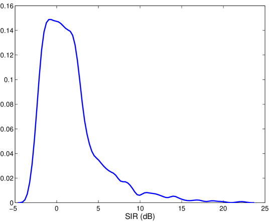
Figure 3: SIR histogram without precoding, pre-fixed BFN.

We have tested the performance of the different schemes in a Monte Carlo simulation for the specifications of a multibeam satellite antenna which uses a fed reflector antenna array with $N=155$ feeds to exchange signals with the users. In particular, we tested adaptive OBBF (labeled as OBBF-adaptive), OBBF with coarse BFN (labeled as OBBF-coarse) and OBBF with pre-fixed matrix (labeled as OBBF-pre-fixed), with the OGBF solution in Section III as reference. As representative example we have chosen the radiation pattern provided by the European Space Agency (ESA) and used in different projects and publications by researchers cooperating in Europe with ESA, see, e.g., [5] and [7]. This radiation pattern is designed to limit the level of interference among users in systems with conservative frequency reuse and a single gateway. As opposed to this, we assume that the whole available bandwidth is used by all beams, resulting in high intra-cluster and inter-cluster interference levels. For the BFN provided by ESA, Figure 3 shows the histogram of the signal to interference ratio (SIR) without precoding for full-frequency reuse, obtained from evaluating the interference for the different users and 100 realizations. For each realization the channel response to 100 users randomly located, one per cluster, is generated. As expected, many users suffer from high interference, especially those which happen to be near the edge of the corresponding beam, given that this BFN is suited for a unique gateway and low co-channel interference associated to a conservative frequency reuse across beams. In the setting under study, the feeder link is shared by $M=10$ gateways, with the corresponding clusters shown in Figure 4. Clusters are groups of ten beams ($k=10$). Each gateway uses only a subset of $n$ feeds, which is chosen by maximizing the average gain for all users in the cluster. The allocated power to all clusters is the same, $P_{m}=P/M$, with $P$ the satellite available transmit power. We assume that the different feeder links are transparent, neglecting the possible impairments in the communication between the gateways and the satellite. The randomness of the Monte Carlo simulation comes from the location of the users at the $K=100$ spot-beams; these locations are chosen from independent uniform distributions inside the different beams, with 100 users being served at each realization, and independently across realizations.

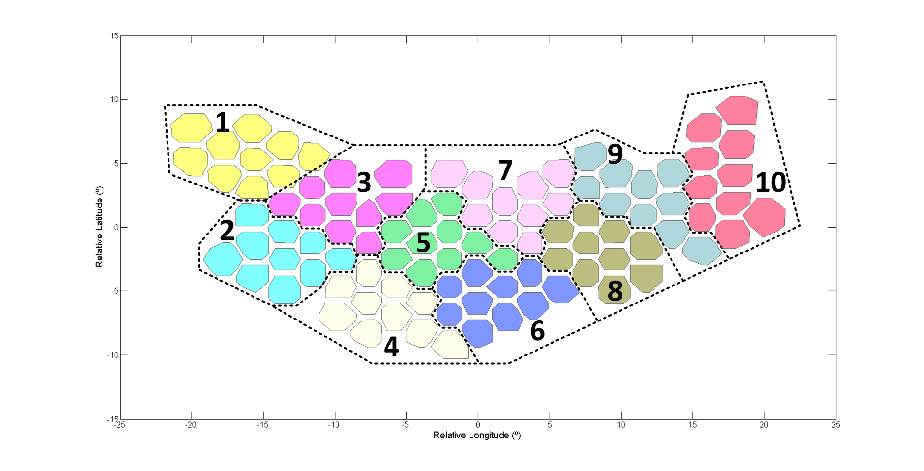
Figure 4: Spot-beams are grouped into clusters.

In order to compare the performance of different schemes the operation point needs to be calibrated. This is set by defining the signal to noise ratio (SNR) as

$$\mathop{\rm SNR}=\mathbb{E}\left[{\operatorname{tr}\{{\mathbf{H}}{\mathbf{F}}{\mathbf{F}}^{H}{\mathbf{H}}^{H}\}}\right]/K$$ (53)

and ${\mathbf{F}}$ the transmit beamforming matrix ${\mathbf{F}}=\frac{\sqrt{P}}{\sqrt{\operatorname{tr}\{{\mathbf{H}}^{H}{\mathbf{H}}\}}}{\mathbf{H}}^{H}$.

Figure 5 presents the average SINR for all users and the different schemes after 50 Monte Carlo realizations. Results have been obtained for two different number of feeds, $n=16$ and $n=30$. Even though all feeds are available to serve any cluster, not more than 35 participate in the provision of power to an arbitrary cluster. The performance is upper bounded by the OGBF scheme, applicable if the gateways have access to the different feeds without an intermediate BFN and the CSIT is perfect. Even further, the OGBF bound for the single gateway case, i.e., $M=1$ and different scaling parameters for all users, is also included to illustrate the performance loss due to the lack of data exchange among gateways. All the other curves use an on-board BFN, either adaptive or fixed; the latter uses either the coarse design in Section IV-D or the BFN provided by ESA for the four-color reuse scheme. As expected, performance improves if more feeds are assigned to each gateway, keeping in mind that feeds can be shared by different gateways. There is a significant loss from the OBBF-adaptive with respect to the OGBF scheme, which increases with the SNR, and which comes from the isolated operation of the gateways. Nevertheless, the degradation of the coarse BFN with respect to the corresponding adaptive BFN version stays below 1dB in all cases, and decreases for low SNR. It is left for future studies whether robustness can be preserved for alternative designs of the BFN able to address the aggregated inter-cluster interference, rather than the noise or the interference to a specific set of users. It can be also noticed that the design of a specific BFN fixed matrix as part of a global multi-gateway interference cancellation scheme provides a gain with respect to a BFN not specifically designed with this in mind, for $n=30$, whereas for $n=16$ this gain is barely noticeable. Additionally, the histogram of SINR is also shown in Figure 6 for both OBBF-adaptive and OGBF schemes, with $n=30$ and SNR = 20dB. With respect to the baseline histogram in Figure 3, a more compact distribution of SINR values is obtained.

As illustration of the role played by the regularization factor in the precoding process, we have also compared the use of different regularization factors in the computation of the precoder for the adaptive BFN case (OBBF-adaptive):

1. $\gamma_{m}=k/P_{m}$. This is the regularization factor minimizing the MSE for a single cluster, as it is well-established in the literature [4].

2. $\gamma_{m}$ the numerical solution of (28), with $\sigma_{ii}^{(m)}$ the $i$th diagonal entry of ${\mathbf{U}}_{m}^{H}{\mathbf{B}}_{m}^{H}\bm{\Sigma}_{m}{\mathbf{B}}_{m}{\mathbf{U}}_{m}$, and $\bm{\Sigma}_{m}$ approximated as (26).

3. $\gamma_{m}$ the numerical solution of (28), with $\sigma_{ii}^{(m)}$ the $i$th diagonal entry of ${\mathbf{U}}_{m}^{H}{\mathbf{B}}_{m}^{H}\hat{\bm{\Sigma}}_{m}{\mathbf{B}}_{m}{\mathbf{U}}_{m}$. This is the regularization factor which has been used to obtain results in Figure 5, which does not require inter-gateway cooperation, since $\hat{\bm{\Sigma}}_{m}$ in (30) is based on average statistics.

4. Closed-form expression (31) to approximate the numerical solution of (28).

The expectation in the last two cases has been approximated empirically. As depicted in Figure 7, which shows the impact of the regularization factor, the inter-cluster solution $k/P_{m}$ falls short of being effective in the presence of intra-cluster interference. More interestingly, the closed form ad-hoc solution matches the performance of the numerically optimized regularization factor. The use of instantaneous channel matrices does not improve significantly the performance, and gives additional merit to the autonomous operation of gateways without permanent exchange of information; only average inter-cluster channel matrices are needed for the implementation of the proposed schemes.

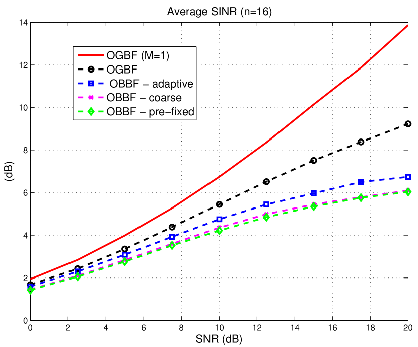
(a) $n=16$.

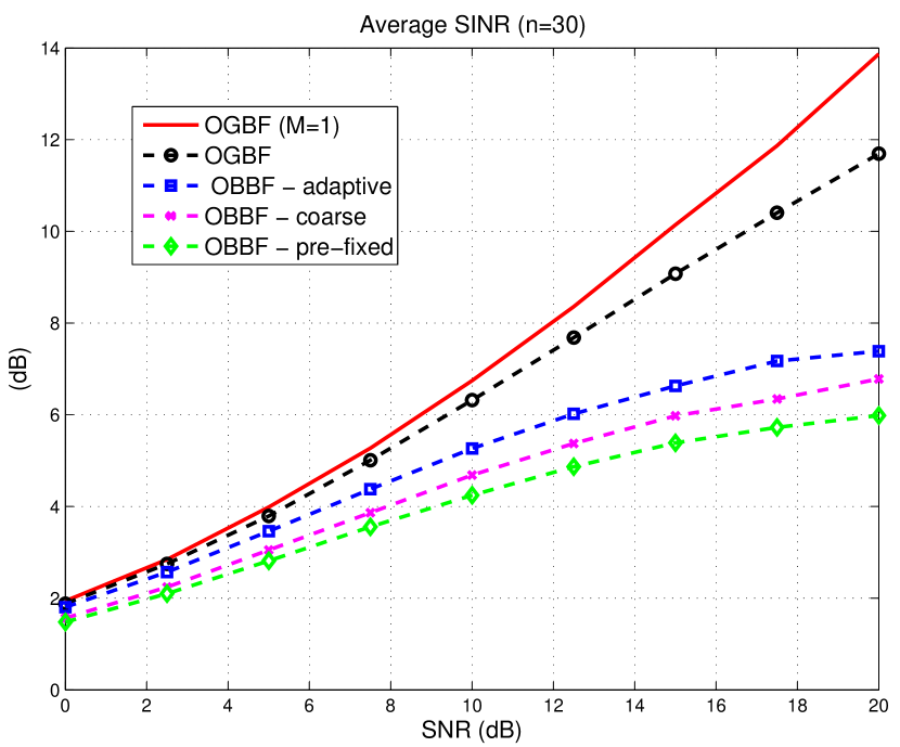
(b) $n=30$.

Figure 5: $M=10,k=10$, 50 realizations. Upper bound: OGBF, one gateway. Lower bound: fixed BFN provided by ESA, distributed precoders.

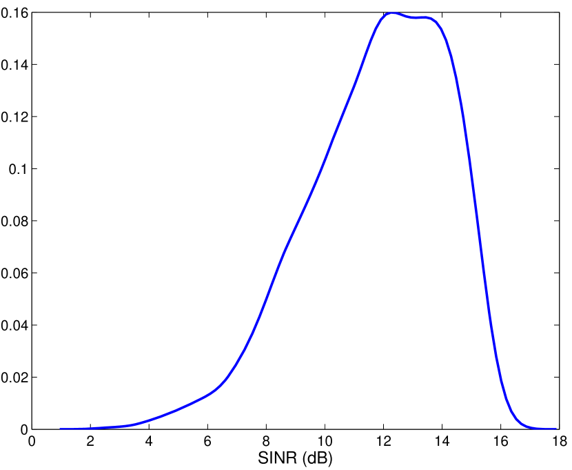
(a) OGBF.

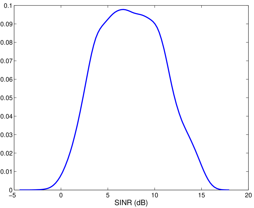
(b) OBBF.

Figure 6: $M=10,k=10,n=30$, SINR histograms based on 50 realizations, SNR = 20dB.

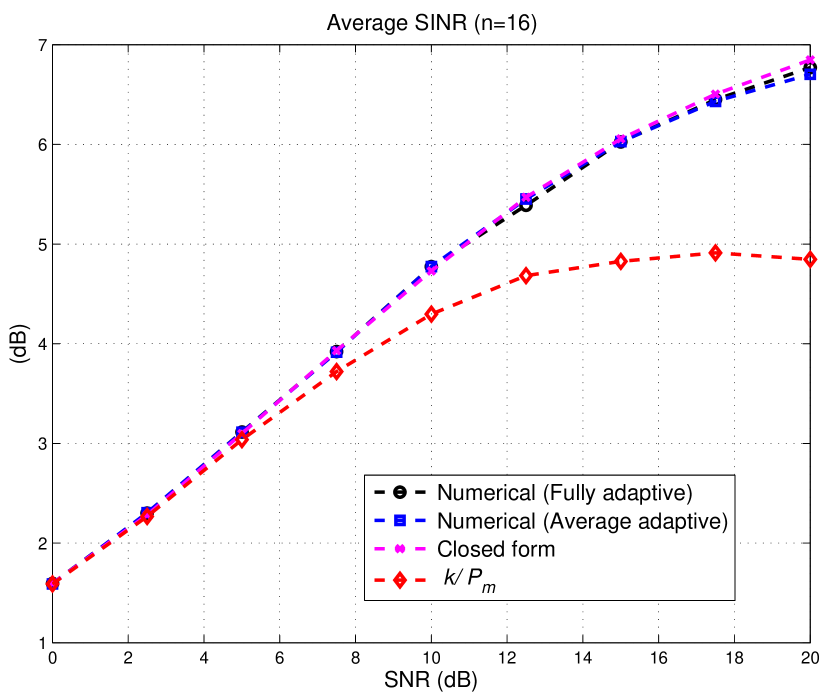
(a) $n=16$.

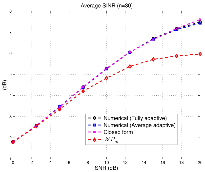
(b) $n=30$.

Figure 7: $M=10,k=10$, 50 realizations. Performance with different regularization factors.

Lastly, we have checked the dispersion of the scalars $\{t_{m}\}$. In order to avoid the interaction among clusters, we have assumed throughout the paper that their values are similar. Otherwise an iterative process to solve the multiple dependencies among $\{{\mathbf{T}}_{m},\gamma_{m},\bm{\Sigma}_{m},t_{m}\}$ would require the sequential exchange of information among the gateways, and make their autonomous optimization unfeasible. Figure 8 shows an average ratio of maximum to minimum values lower than 2 for the two settings addressed in the previous simulations, supporting the allocation of similar weights to all the inter-cluster Gramians in (26).

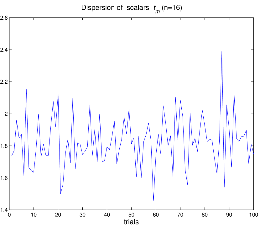
(a) $n=16$.

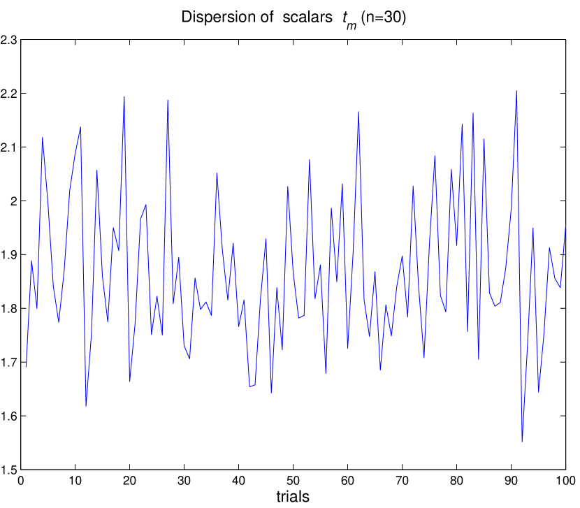
(b) $n=30$.

Figure 8: $\max_{m}\{t_{m}\}/\min_{m}\{t_{m}\}$ for different trials. $M=10,k=10$, SNR = 10dB.

VI Conclusions

The mitigation of co-channel interference in multibeam satellite settings has been addressed in this paper, for the case of several ground stations using the satellite to relay their signals to their respective clusters of beams. Both sources of interference, intra-cluster and inter-cluster, are attenuated by considering the global MSE and deriving distributed on-ground linear precoders and on-board beamforming weights. Practical rules have been provided to design the on-ground precoders and on-board beamformer for different degrees of flexibility of the latter, including also a coarse fixed BFN. Under the premise of no cooperation among gateways, the regularization factor of the MMSE precoders was obtained, first numerically and then in an approximated closed form, to account for the presence of inter-cluster leakage, generalizing existing results for a centralized precoder. For the purpose of benchmarking an On-Groud Beamforming solution has been derived with full flexibility. Exploration of non-linear schemes of the type Tomlinson-Harashima to improve the rate, as proposed in [18] in combination with regularization at the transmit precoder, can be a topic for further improvement of the results exposed in this paper, together with the consideration of CSI errors in the design of the ground precoders. The design of the BFN can be also extended to account for the aggregated inter-cluster leakage; the key performance indicator will be the ability to mitigate the interference with a fixed design, given that a well-performing adaptive solution does not necessarily lead to a valid robust design.

Appendix A Numerical finding of Lagrange multiplier for OGBF design

Consider the problem

$$\min_{{\mathbf{F}}}\operatorname{tr}\{{\mathbf{F}}^{H}{\mathbf{A}}{\mathbf{F}}-{\mathbf{F}}^{H}{\mathbf{X}}-{\mathbf{X}}^{H}{\mathbf{F}}\}\quad\text{subject to}\quad\operatorname{tr}\{{\mathbf{F}}^{H}{\mathbf{F}}^{H}\}\leq P,$$ (54)

with ${\mathbf{A}}\in\mathbb{C}^{n\times n}$ Hermitian positive definite, and ${\mathbf{F}},{\mathbf{X}}\in\mathbb{C}^{n\times k}$.

Let ${\mathbf{A}}={\mathbf{U}}\bm{\Gamma}{\mathbf{U}}^{H}$ be the eigenvalue decomposition of ${\mathbf{A}}$, and define $\tilde{\mathbf{F}}={\mathbf{U}}^{H}{\mathbf{F}},\tilde{\mathbf{X}}={\mathbf{U}}^{H}{\mathbf{X}}$. Since ${\mathbf{U}}\in\mathbb{C}^{n\times n}$ is unitary, we can reformulate (54) as

$$\min_{{\mathbf{F}}}\operatorname{tr}\{\tilde{\mathbf{F}}^{H}\bm{\Gamma}\tilde{\mathbf{F}}-\tilde{\mathbf{F}}^{H}\tilde{\mathbf{X}}-\tilde{\mathbf{X}}^{H}\tilde{\mathbf{F}}\}\quad\text{subject to}\quad\operatorname{tr}\{\tilde{\mathbf{F}}^{H}\tilde{\mathbf{F}}^{H}\}\leq P.$$ (55)

Assuming that the unconstrained solution $\tilde{\mathbf{F}}=\bm{\Gamma}^{-1}\tilde{\mathbf{X}}$ is not feasible (which must be checked), then the constraint must be satisfied with equality with $\tilde{\mathbf{F}}=(\bm{\Gamma}+\nu{\mathbf{I}}_{n})^{-1}\tilde{\mathbf{X}}$:

$$\operatorname{tr}\{\tilde{\mathbf{F}}^{H}\tilde{\mathbf{F}}\}=\operatorname{tr}\{\tilde{\mathbf{X}}^{H}(\bm{\Gamma}+\nu{\mathbf{I}}_{n})^{-2}\tilde{\mathbf{X}}\}=P.$$ (56)

Let $\bm{\Gamma}=\text{diag}\{\begin{array}[]{cccc}\gamma_{1}&\gamma_{2}&\cdots&\gamma_{n}\}\end{array}$, and write $\tilde{\mathbf{X}}$ row-wise as

$$\tilde{\mathbf{X}}=\left[\begin{array}[]{c}\tilde{\mathbf{x}}_{1}^{H}\\ \tilde{\mathbf{x}}_{2}^{H}\\ \vdots\\ \tilde{\mathbf{x}}_{n}^{H}\end{array}\right].$$ (57)

Then

$$\operatorname{tr}\{\tilde{\mathbf{X}}^{H}(\bm{\Gamma}+\nu{\mathbf{I}}_{n})^{-2}\tilde{\mathbf{X}}\}=\sum_{i=1}^{n}\frac{\tilde{\mathbf{x}}_{i}^{H}\tilde{\mathbf{x}}_{i}}{(\gamma_{i}+\nu)^{2}}=\phi(\nu).$$ (58)

Thus, the Lagrange multiplier must satisfy $\phi(\nu)=P$. Note that $\phi(0)>P$ (because otherwise the unconstrained solution would be feasible) and that $\phi(\nu)$ is monotone decreasing for $\nu>0$, with $\lim_{\nu\rightarrow\infty}\phi(\nu)=0$; therefore there is a unique positive solution of $\phi(\nu)=P$, which can be found by bisection, Newton’s method, or any root-finding technique.

Appendix B Derivation of regularization factor for on-ground precoders

We start with the decomposition ${\mathbf{B}}_{m}^{H}{\mathbf{H}}_{mm}^{H}{\mathbf{H}}_{mm}{\mathbf{B}}_{m}={\mathbf{U}}_{m}{\mathbf{S}}_{m}{\mathbf{U}}_{m}^{H}$, which for the adaptive BFN in Section IV-B boils down to ${\mathbf{S}}_{H,m}$ in (38). The error term (25) is expressed as

$$\operatorname{tr}\{{\mathbf{E}}_{m}\}=\operatorname{tr}\{{\mathbf{I}}_{k}\}-2\operatorname{tr}\{({\mathbf{U}}_{m}{\mathbf{S}}_{m}{\mathbf{U}}_{m}^{H}+\gamma_{m}{\mathbf{I}}_{k})^{-1}{\mathbf{U}}_{m}{\mathbf{S}}_{m}{\mathbf{U}}_{m}^{H}\}\\ +\operatorname{tr}\{({\mathbf{U}}_{m}{\mathbf{S}}_{m}{\mathbf{U}}_{m}^{H}+\gamma_{m}{\mathbf{I}}_{k})^{-1}({\mathbf{U}}_{m}{\mathbf{S}}_{m}{\mathbf{U}}_{m}^{H}+{\mathbf{B}}_{m}\bm{\Sigma}_{m}{\mathbf{B}}_{m})({\mathbf{U}}_{m}{\mathbf{S}}_{m}{\mathbf{U}}_{m}^{H}+\gamma_{m}{\mathbf{I}}_{k})^{-1}{\mathbf{U}}_{m}{\mathbf{S}}_{m}{\mathbf{U}}_{m}^{H}\}\\ +\operatorname{tr}\left\{\frac{1}{t_{m}}{\mathbf{I}}_{k}\right\}$$ (59)

which, by using the orthonormality of ${\mathbf{U}}_{m}$, can be alternatively expressed as

$$\operatorname{tr}\{{\mathbf{E}}_{m}\}=k-2\operatorname{tr}\left\{({\mathbf{S}}_{m}+\gamma_{m}{\mathbf{I}}_{k})^{-1}{\mathbf{S}}_{m}\right\}+\operatorname{tr}\left\{({\mathbf{S}}_{m}+\gamma_{m}{\mathbf{I}}_{k})^{-1}\cdot\right.\\ \left.({\mathbf{S}}_{m}+{\mathbf{U}}_{m}^{H}{\mathbf{B}}_{m}^{H}\bm{\Sigma}_{m}{\mathbf{B}}_{m}{\mathbf{U}}_{m})({\mathbf{S}}_{m}+\gamma_{m}{\mathbf{I}}_{k})^{-1}{\mathbf{S}}_{m}\right\}+k/t_{m}.$$ (60)

The scaling $t_{m}$ in the last term is obtained from the power constraint in (24) and the precoder expression (23):

$$t_{m}=\frac{P_{m}}{\operatorname{tr}\left\{({\mathbf{B}}_{m}^{H}{\mathbf{H}}_{mm}^{H}{\mathbf{H}}_{mm}{\mathbf{B}}_{m}+\gamma_{m}{\mathbf{I}}_{k})^{-1}{\mathbf{B}}_{m}^{H}{\mathbf{H}}_{mm}^{H}{\mathbf{H}}_{mm}{\mathbf{B}}_{m}({\mathbf{B}}_{m}^{H}{\mathbf{H}}_{mm}^{H}{\mathbf{H}}_{mm}{\mathbf{B}}_{m}+\gamma_{m}{\mathbf{I}}_{k})^{-1}\right\}},$$ (61)

or, equivalently,

$$t_{m}=\frac{P_{m}}{\operatorname{tr}\left\{({\mathbf{S}}_{m}+\gamma_{m}{\mathbf{I}}_{k})^{-1}{\mathbf{S}}_{m}({\mathbf{S}}_{m}+\gamma_{m}{\mathbf{I}}_{k})^{-1}\right\}}.$$ (62)

If we insert this into $\operatorname{tr}\{{\mathbf{E}}_{m}\}$, then we have the following minimization problem:

$$\gamma_{m}=\arg\min\sum_{i=1}^{k}\frac{-2\lambda_{i}^{(m)}}{\lambda_{i}^{(m)}+\gamma_{m}}+\frac{(\lambda_{i}^{(m)})^{2}}{(\lambda_{i}^{(m)}+\gamma_{m})^{2}}+\frac{\sigma_{ii}^{(m)}\lambda_{i}^{(m)}}{(\lambda_{i}^{(m)}+\gamma_{m})^{2}}+\frac{k}{P_{m}}\frac{\lambda_{i}^{(m)}}{(\lambda_{i}^{(m)}+\gamma_{m})^{2}}$$ (63)

where $\sigma_{ii}^{(m)}$ is the $i$th diagonal entry of ${\mathbf{U}}_{m}^{H}{\mathbf{B}}_{m}^{H}\bm{\Sigma}_{m}{\mathbf{B}}_{m}{\mathbf{U}}_{m}$, and $\lambda_{i}^{(m)}$ the $i$th eigenvalue of ${\mathbf{B}}_{m}^{H}{\mathbf{H}}_{mm}^{H}{\mathbf{H}}_{mm}{\mathbf{B}}_{m}$. By equating to zero the derivative the relation to satisfy is

$$\sum_{i=1}^{k}\frac{\lambda_{i}^{(m)}}{(\lambda_{i}^{(m)}+\gamma_{m})^{3}}\left(\gamma_{m}-\sigma_{ii}^{(m)}-\frac{k}{P_{m}}\right)=0$$ (64)

and the scaling parameter

$$t_{m}=P_{m}/\sum_{i=1}^{k}\frac{\lambda_{i}^{(m)}}{(\lambda_{i}^{(m)}+\gamma_{m})^{2}}.$$ (65)

References

• [1] D. Minoli, Innovations in Satellite Communications Technology.   John Wiley & Sons, Inc., Hoboken, NJ, USA, 2015.
• [2] J. Tronc, P. Angeletti, N. Song, M. Haardt, J. Arendt, and G. Gallinaro, “Overview and comparison of on-ground and on-board beamforming techniques in mobile satellite service applications,” International Journal of Satellite Communications and Networking, vol. 32, no. 4, pp. 291–308, 2014.
• [3] G. Zheng, S. Chatzinotas, and B. Ottersten, “Multi-gateway cooperation in multibeam satellite systems,” in 2012 IEEE 23rd International Symposium on Personal, Indoor and Mobile Radio Communications-(PIMRC).   IEEE, 2012, pp. 1360–1364.
• [4] C. B. Peel, B. M. Hochwald, and A. L. Swindlehurst, “A vector-perturbation technique for near-capacity multiantenna multiuser communication-part I: channel inversion and regularization,” IEEE Transactions on Communications, vol. 53, no. 1, pp. 195–202, Jan 2005.
• [5] B. Devillers, A. Pérez-Neira, and C. Mosquera, “Joint linear precoding and beamforming for the forward link of multi-beam broadband satellite systems,” in Global Telecommunications Conference (GLOBECOM 2011), 2011 IEEE.
• [6] S. Chatzinotas, B. Ottersten, and R. De Gaudenzi, Cooperative and cognitive satellite systems.   Academic Press, 2015.
• [7] V. Joroughi, M. A. Vázquez, and A. I. Pérez-Neira, “Precoding in multigateway multibeam satellite systems,” IEEE Transactions on Wireless Communications, vol. 15, no. 7, pp. 4944–4956, July 2016.
• [8] M. Sadek, A. Tarighat, and A. H. Sayed, “A leakage-based precoding scheme for downlink multi-user MIMO channels,” IEEE Transactions on Wireless Communications, vol. 6, no. 5, pp. 1711–1721, May 2007.
• [9] P. Patcharamaneepakorn, S. Armour, and A. Doufexi, “On the equivalence between SLNR and MMSE precoding schemes with single-antenna receivers,” IEEE Communications Letters, vol. 16, no. 7, pp. 1034–1037, July 2012.
• [10] B. K. Chalise and L. Vandendorpe, “Optimization of MIMO relays for multipoint-to-multipoint communications: Nonrobust and robust designs,” IEEE Transactions on Signal Processing, vol. 58, no. 12, pp. 6355–6368, 2010.
• [11] P. Stoica and Y. Selén, “Cyclic minimizers, majorization techniques, and the expectation-maximization algorithm: a refresher,” IEEE Signal Processing Magazine, vol. 21, no. 1, pp. 112–114, 2004.
• [12] C. K. Wen, J. C. Chen, K. K. Wong, and P. Ting, “Message passing algorithm for distributed downlink regularized zero-forcing beamforming with cooperative base stations,” IEEE Transactions on Wireless Communications, vol. 13, no. 5, pp. 2920–2930, May 2014.
• [13] C. Mosquera, R. López-Valcarce, and T. Ramírez, “Distributed precoding systems in multi-gateway multibeam satellites,” 2017, submitted to 14th International Symposium on Wireless Communication Systems.
• [14] C. R. J. R. A. Horn, Matrix Analysis, 2nd ed.   Cambridge University Press, 2013.
• [15] B. Devillers and A. Pérez-Neira, “Advanced interference mitigation techniques for the forward link of multi-beam broadband satellite systems,” in 2011 Conference Record of the Forty Fifth Asilomar Conference on Signals, Systems and Computers (ASILOMAR).   IEEE, 2011, pp. 1810–1814.
• [16] Y. C. Silva and A. Klein, “Linear transmit beamforming techniques for the multigroup multicast scenario,” IEEE Transactions on Vehicular Technology, vol. 58, no. 8, pp. 4353–4367, 2009.
• [17] Q. H. Spencer, A. L. Swindlehurst, and M. Haardt, “Zero-forcing methods for downlink spatial multiplexing in multiuser MIMO channels,” IEEE Transactions on Signal Processing, vol. 52, no. 2, pp. 461–471, 2004.
• [18] B. M. Hochwald, C. B. Peel, and A. L. Swindlehurst, “A vector-perturbation technique for near-capacity multiantenna multiuser communication-part II: perturbation,” IEEE Transactions on Communications, vol. 53, no. 3, pp. 537–544, March 2005.