Exact adaptive confidence intervals for linear regression coefficients

Abstract

We propose an adaptive confidence interval procedure (CIP) for the coefficients in the normal linear regression model. This procedure has a frequentist coverage rate that is constant as a function of the model parameters, yet provides smaller intervals than the usual interval procedure, on average across regression coefficients. The proposed procedure is obtained by defining a class of CIPs that all have exact $1-\alpha$ frequentist coverage, and then selecting from this class the procedure that minimizes a prior expected interval width. Such a procedure may be described as “frequentist, assisted by Bayes” or FAB. We describe an adaptive approach for estimating the prior distribution from the data so that exact non-asymptotic $1-\alpha$ coverage is maintained. Additionally, in a “$p$ growing with $n$” asymptotic scenario, this adaptive FAB procedure is asymptotically Bayes-optimal among $1-\alpha$ frequentist CIPs.

Keywords: empirical Bayes, frequentist coverage, ridge regression, shrinkage, sparsity.

1 Introduction

Linear regression analyses routinely include point estimates and confidence intervals for the regression coefficients ${\boldsymbol{\beta}}=(\beta_{1},\ldots,\beta_{p})$ of the linear model ${\mathbf{y}}\sim N_{n}({\mathbf{X}}{\boldsymbol{\beta}},\sigma^{2}{\mathbf{I}})$. The most widely-used confidence interval procedure (CIP) for an element $\beta_{j}$ of ${\boldsymbol{\beta}}$ is perhaps the usual $t$-interval centered around the ordinary least-squares (OLS) estimate $\hat{\beta}_{j}$. This interval is uniformly most accurate among CIPs that are derived from inversion of unbiased tests, and so it is called the uniformly most accurate unbiased (UMAU) CIP.

In this article we consider alternatives to the UMAU procedure that have constant coverage, that is, interval procedures $C_{j}({\mathbf{y}})$ satisfying

$$\Pr(\beta_{j}\in C_{j}({\mathbf{y}})|{\boldsymbol{\beta}},\sigma)=1-\alpha,\ \forall\,({\boldsymbol{\beta}},\sigma)\in\mathbb{R}^{p}\times\mathbb{R}^{+}.$$ (1)

This property is what we normally think of as the usual frequentist definition of $1-\alpha$ coverage - the random interval $C_{j}({\mathbf{y}})$ covers the true value $\beta_{j}$ with probability $1-\alpha$, no matter what ${\boldsymbol{\beta}}$ and $\sigma$ are. We introduce the term “constant coverage” to distinguish such intervals from other intervals whose coverage is bounded below by $1-\alpha$ but varies with $({\boldsymbol{\beta}},\sigma^{2})$, or so-called “frequentist intervals” whose coverage rate is only constant as a function of the parameters asymptotically. For example, the usual score interval for a coefficient in a logistic regression model has an actual finite-sample coverage rate that depends on the values of the parameters.

The UMAU interval procedure of course has constant coverage, and it also has an expected width that is constant for all values of ${\boldsymbol{\beta}}$. However, in many cases we have prior information that many of the elements of ${\boldsymbol{\beta}}$ may be close to a particular value, such as zero. In this case, we might prefer a CIP for $\beta_{j}$ that has a smaller expected width for “likely” values of $\beta_{j}$ in exchange for having wider intervals for values of $\beta_{j}$ that are less likely. Specifically, if our prior information could be quantified in terms of a prior distribution with density $\pi({\boldsymbol{\beta}})$, then arguably we would be interested in an interval procedure that minimizes the prior expected width

$${\text{E}}[|C_{j}({\mathbf{y}})|]=\int\int|C_{j}({\mathbf{y}})|\,p({\mathbf{y}}|{\boldsymbol{\beta}},\sigma)\,d{\mathbf{y}}\,\pi({\boldsymbol{\beta}})d{\boldsymbol{\beta}}$$

among all CIPs that satisfy the constant coverage property (1). Such a procedure would still be “frequentist” in that it would have $1-\alpha$ constant coverage, but it would also be Bayes-optimal among frequentist procedures. We refer to such a statistical procedure as “frequentist, assisted by Bayes” or FAB.

In practice, an appropriate prior distribution may not be known in advance. In this article we present a method for adaptively estimating a normal prior distribution for ${\boldsymbol{\beta}}$ from the data ${\mathbf{y}}$, and then using this estimated prior distribution to construct an approximately Bayes-optimal CIP for each regression coefficient $\beta_{j},j=1,\ldots,p$. The CIP we propose satisfies the constant coverage condition (1) exactly and non-asymptotically, but it is also Bayes-optimal asymptotically as $p$ and $n$ increase to infinity. Our proposed adaptive CIP builds on the work of Pratt (1963), who obtained a Bayes-optimal frequentist confidence interval for the mean of a normal population with a known variance. In the next section we review Pratt’s FAB interval, and discuss an extension developed in Yu and Hoff (2016) to accommodate an unknown variance. In Section 3 we further extend these ideas to the case of interval estimation for a linear regression coefficient, and show how we may adaptively estimate a normal prior distribution for the elements of ${\boldsymbol{\beta}}$. The resulting adaptive FAB confidence interval we propose maintains exact, non-asymptotic constant coverage. Additionally, since the accuracy of our adaptive estimate improves as $n$ and $p$ increase, our adaptive FAB procedure is Bayes-optimal under this type of asymptotic regime. Section 4 includes several numerical examples illustrating the use of the adaptive FAB procedure, including analyses of two datasets and a small simulation study. A discussion follows in Section 5.

Several other authors have studied alternatives to UMAU intervals for regression parameters. O’Gorman (2001) developed a CIP based on a permutation test that adapts to non-normal error distributions, as opposed to adapting to small or sparse values of the regression coefficients. Kabaila and Tissera (2014) developed an improved CIP based on an adaptive estimate of the variance $\sigma^{2}$. Their procedure depends on a user-specified spline function for which the constant coverage property must be checked numerically. In contrast, our proposed CIP is obtained by adaptively selecting from a class of constant-coverage intervals based on easy to obtain estimates of a few parameters. For our procedure, constant coverage follows by construction and does not need to be checked numerically. Lee et al. (2016) developed a procedure that has exact conditional coverage, given a model selection event and knowledge of $\sigma^{2}$. However, for cases where $\sigma^{2}$ is unknown, their suggested modification uses a plug-in estimate of $\sigma^{2}$ and achieves exact coverage only asymptotically. Other authors (Bühlmann (2013), van de Geer et al. (2014), Zhang and Zhang (2014)) have considered confidence interval construction for sparse, high-dimensional regression, including the case that $p>n$. These approaches generally work by de-biasing sparse estimators of the regression coefficients. However, the coverage rates of these methods are asymptotic, and typically depend on conditions on the design matrix ${\mathbf{X}}$ and the degree of sparsity of ${\boldsymbol{\beta}}$. For example, in Section 4 we show that the finite-sample coverage of one such procedure can be very good in a sparse setting, but extremely poor if ${\boldsymbol{\beta}}$ is not sparse.

2 Review of FAB intervals

Suppose $\hat{\theta}$ is normally distributed with unknown mean $\theta$ and known variance $\sigma^{2}$. Then for any choice of $s\in[0,1]$,

$$\ \Pr(z_{\alpha(1-s)}<(\theta-\hat{\theta})/\sigma<z_{1-\alpha s}|\theta) =(1-\alpha s)-\alpha(1-s)$$

$$=1-\alpha,$$

where $z_{p}$ denotes the $p$th quantile of the standard normal distribution. As described in Yu and Hoff (2016), this implies that for any function $s:\mathbb{R}\rightarrow[0,1]$ the set-valued function

$$C_{s}(\hat{\theta})=\left\{\theta:\hat{\theta}+\sigma z_{\alpha(1-s(\theta))}<\theta<\hat{\theta}+\sigma z_{1-\alpha s(\theta)}\right\}$$ (2)

is a $1-\alpha$ confidence procedure, satisfying $\Pr(\theta\in C_{s}(\hat{\theta})|\theta)=1-\alpha$. We refer to such a function $s(\theta)$ as a spending function, as it corresponds to regions of the parameter space upon which type I error is “spent.”

The usual procedure is $C_{1/2}(\hat{\theta})$, obtained from the constant spending function $s(\theta)=1/2$. While $C_{1/2}$ is the uniformly most accurate unbiased (UMAU) confidence interval procedure (CIP), the lack of a uniformly most powerful test of $H_{\theta}:{\text{E}}[\hat{\theta}]=\theta$ versus $K_{\theta}:{\text{E}}[\hat{\theta}]\neq\theta$ means there are confidence procedures corresponding to collections of biased level-$\alpha$ tests that have smaller expected widths than the UMAU procedure for some regions of the parameter space. If prior information is available that $\theta$ is likely to be near some value $\mu$, then we may be willing to incur wider intervals for $\theta$-values far from $\mu$ in exchange for smaller intervals near $\mu$. With this in mind, Pratt (1963) developed a Bayes-optimal $1-\alpha$ CIP that minimizes the “Bayes width” or expected interval width averaged over values of both $\hat{\theta}$ and $\theta$, where the latter averaging is done with respect to a $N(\mu,\tau^{2})$ prior distribution for $\theta$. The resulting CIP has $1-\alpha$ frequentist coverage for each value of $\theta$, but has lower expected width for values of $\theta$ near the prior mean (and wider expected widths elsewhere). We describe this interval as being “frequentist assisted by Bayes” or FAB. As shown in Yu and Hoff (2016), the spending function corresponding to Pratt’s FAB confidence interval is characterized as follows: If $\tau^{2}>0$, then

$$s(\theta) =g^{-1}(2\sigma(\theta-\mu)/\tau^{2})$$ (3)

$$g(s) =\Phi^{-1}(\alpha s)-\Phi^{-1}(\alpha(1-s)).$$

If $\tau^{2}=0$, then $s(\theta)=1$ if $\theta>\mu$ and $s(\theta)<0$ if $\theta<\mu$. The value of $s(\mu)\in[0,1]$ does not affect the width of the confidence interval, but can affect whether or not $\mu$ is included in the interval or not (as an endpoint). We suggest taking $s(\mu)$ to be 1/2 when $\tau^{2}=0$, as it is in the case that $\tau^{2}>0$.

Now consider confidence interval construction for $\theta$ in the more typical case that $\sigma^{2}$ is unknown. Suppose we will observe independent statistics $\hat{\theta}$ and $\hat{\sigma}^{2}$, where $\hat{\theta}\sim N(\theta,\sigma^{2})$ and $q\hat{\sigma}^{2}/\sigma^{2}\sim\chi^{2}_{q}$. Letting $t_{p}$ be the $p$th quantile of the $t$-distribution with $q$ degrees of freedom, any spending function $s:\mathbb{R}\rightarrow[0,1]$ defines a class of acceptance regions

$$A_{s}(\theta)=\left\{(\hat{\theta},\hat{\sigma}):\hat{\theta}+\hat{\sigma}t_{\alpha(1-s(\theta))}<\theta<\hat{\theta}+\hat{\sigma}t_{1-\alpha s(\theta)}\right\},$$

so that for each $\theta$, $A_{s}(\theta)$ is the acceptance region of a level-$\alpha$ test. Inversion of this class of tests yields a CIP with exact $1-\alpha$ constant coverage,

$$C_{s}(\hat{\theta},\hat{\sigma})=\left\{\theta:\hat{\theta}+\hat{\sigma}t_{\alpha(1-s(\theta))}<\theta<\hat{\theta}+\hat{\sigma}t_{1-\alpha s(\theta)}\right\}.$$ (4)

Important properties of this CIP include the following:

Theorem 1.

If $\hat{\theta}\sim N(\theta,\sigma^{2})$ and $q\hat{\sigma}^{2}/\sigma^{2}\sim\chi^{2}_{q}$ are independent, then

1. $\Pr(\theta\in C_{s}(\hat{\theta},\hat{\sigma})|\theta,\sigma)=1-\alpha\,\forall\,(\theta,\sigma)\in\mathbb{R}\times\mathbb{R}^{+}$, so the procedure has $1-\alpha$ constant coverage;

2. If $s(\theta)$ is nondecreasing then $C_{s}(\hat{\theta},\hat{\sigma})$ is an interval with probability 1;

3. If $s(\theta)$ is not nondecreasing then $C_{s}(\hat{\theta},\hat{\sigma})$ is an interval with probability less than 1.

Items 1 and 2 were shown in Yu and Hoff (2016), and a proof of item 3 is in the appendix. This result says that every spending function corresponds to a $1-\alpha$ frequentist confidence procedure, and every nondecreasing spending function corresponds to a $1-\alpha$ confidence interval procedure. Yu and Hoff (2016) showed that the spending function (3) that corresponds to Pratt’s $z$-interval is strictly increasing. If such a nondecreasing spending function $s$ is used, then the lower and upper endpoints of the interval, $\underline{\theta}$ and $\overline{\theta}$, are obtained by solving the equations

$$F\left(\tfrac{\underline{\theta}-\hat{\theta}}{\hat{\sigma}}\right)=\alpha(1-s(\underline{\theta})),\ \ \ \ F\left(\tfrac{\hat{\theta}-\overline{\theta}}{\hat{\sigma}}\right)=\alpha s(\overline{\theta}),$$ (5)

where $F$ is the CDF of the $t_{q}$ distribution. These equations can be solved using a zero-finding algorithm, and noting that $\underline{\theta}<\hat{\theta}+\hat{\sigma}t_{\alpha}$ and $\hat{\theta}+\hat{\sigma}t_{1-\alpha}<\overline{\theta}$. Furthermore, this implies that $\underline{\theta}<\hat{\theta}<\overline{\theta}$ as long as $\alpha<1/2$.

The spending function $s(\theta)$ should be chosen on the basis of any additional information we may have about the value of $\theta$. While Pratt’s FAB interval uses prior information for a scalar parameter, in multiparameter settings such information may come from the data itself. For example, estimates of some parameters might suggest plausible values for others. In this case, we may want to use a spending function $\tilde{s}(\theta)$ that minimizes a Bayes risk corresponding to a “prior” distribution that is adaptively estimated from the data. We refer to such as procedure as adaptive FAB. Fortunately, the results of Proposition 1 hold not just for fixed spending functions, but also those that are random but statistically independent of $\hat{\theta}$ and $\hat{\sigma}^{2}$:

Corollary 1.

If $\hat{\theta}\sim N(\theta,\sigma^{2})$ and $q\hat{\sigma}^{2}/\sigma^{2}\sim\chi^{2}_{q}$, and $\hat{\theta}$, $\hat{\sigma}^{2}$ and $\tilde{s}$ are independent, then $\Pr(\theta\in C_{\tilde{s}}(\hat{\theta},\hat{\sigma})|\theta,\sigma)=1-\alpha$.

This result follows by conditioning on $\tilde{s}$: $\Pr(\theta\in C_{\tilde{s}}(\hat{\theta},\hat{\sigma})|\theta,\sigma)={\text{E}}[\Pr(\theta\in C_{\tilde{s}}(\hat{\theta},\hat{\sigma})|\tilde{s},\theta,\sigma)|\theta,\sigma]$, but the inner conditional probability is $1-\alpha$ since $\tilde{s}$ and $(\hat{\theta},\hat{\sigma})$ are independent and $C_{\tilde{s}}$ has $1-\alpha$ coverage for each fixed $\tilde{s}$. Yu and Hoff (2016) made use of this fact to develop an adaptive FAB confidence interval procedure for the means of multiple normal populations. Their adaptive procedure for the mean $\theta$ of a given population is $C_{\tilde{s}}(\hat{\theta},\hat{\sigma})$, where $\tilde{s}$ is the spending function (3) with $(\mu,\sigma^{2},\tau^{2})$ replaced by estimates using data from the other populations. This procedure provides exact $1-\alpha$ confidence intervals for each population, and is asymptotically optimal in the case of the normal hierarchical model.

3 FAB $t$-intervals for regression parameters

We now show how the results discussed in the previous section may be used to construct adaptive frequentist confidence intervals for linear regression parameters. The intervals we construct have exact $1-\alpha$ constant coverage and do not require asymptotic approximations or assumptions on the design matrix or the unknown parameters. Under some conditions, the intervals are also asymptotically Bayes-optimal. The intervals do require that the number $n$ of observations is larger than the number $p$ of regressors.

3.1 FAB regression intervals

Consider the problem of constructing confidence intervals for the elements of an unknown vector ${\boldsymbol{\beta}}\in\mathbb{R}^{p}$ based on data ${\mathbf{y}}\in\mathbb{R}^{n}$ and ${\mathbf{X}}\in\mathbb{R}^{n\times p}$ from the normal linear regression model ${\mathbf{y}}\sim N_{n}({\mathbf{X}}{\boldsymbol{\beta}},\sigma^{2}{\mathbf{I}})$. As is well known,

$$\hat{{\boldsymbol{\beta}}} =({\mathbf{X}}^{\top}{\mathbf{X}})^{-1}{\mathbf{X}}^{\top}{\mathbf{y}}\sim N_{p}({\boldsymbol{\beta}},\sigma^{2}({\mathbf{X}}^{\top}{\mathbf{X}})^{-1})$$

$$\hat{\sigma}^{2}\ =||{\mathbf{y}}-{\mathbf{X}}\hat{{\boldsymbol{\beta}}}||^{2}/(n-p)\sim\tfrac{\sigma^{2}}{n-p}\chi^{2}_{n-p},$$

with $\hat{{\boldsymbol{\beta}}}$ and $\hat{\sigma}^{2}$ being independent. In particular, $(\hat{\beta}_{j}-\beta_{j})/(w_{j}\hat{\sigma})\sim t_{n-p}$, where $w_{j}$ is the square-root of the $j$th diagonal entry of $({\mathbf{X}}^{\top}{\mathbf{X}})^{-1}$. The UMAU confidence interval for $\beta_{j}$ is

$$C(\hat{\beta}_{j},\hat{\sigma})=\left\{\beta_{j}:\hat{\beta}_{j}+w_{j}\hat{\sigma}t_{\alpha/2}<\beta_{j}<\hat{\beta}_{j}+w_{j}\hat{\sigma}t_{1-\alpha/2}\right\}.$$ (6)

This interval has $1-\alpha$ coverage probability and an expected width that is constant as a function of the true value of $\beta_{j}$.

Now suppose that prior information about ${\boldsymbol{\beta}}$ suggests that ${\boldsymbol{\beta}}\sim N_{p}({\mathbf{0}},\tau^{2}{\mathbf{I}})$ for some value of $\tau^{2}$ (other prior distributions will be discussed in Sections 4 and 5). If $\tau^{2}$ and $\sigma^{2}$ were known, the Bayes-optimal CIP for $\beta_{j}$ would be obtained simply by replacing $\hat{\theta}$ and $\sigma$ in (2) and (3) with $\hat{\beta}_{j}$ and $w_{j}\sigma$, yielding

$$C_{s}(\hat{\beta}_{j}) =\left\{\beta_{j}:\hat{\beta}_{j}+w_{j}\sigma z_{\alpha(1-s(\beta_{j}))}<\beta_{j}<\hat{\beta}_{j}+w_{j}\sigma z_{1-\alpha s(\beta_{j})}\right\}$$ (7)

$$s(\beta_{j}) =g^{-1}(2w_{j}\sigma\beta_{j}/\tau^{2}).$$

However, since $\tau^{2}$ and $\sigma^{2}$ are unknown we alter this interval as follows:

• $\sigma^{2}$ is replaced by $\hat{\sigma}^{2}$, which is independent of $\hat{\beta}_{j}$ and satisfies $(n-p)\hat{\sigma}^{2}/\sigma^{2}\sim\chi^{2}_{n-p}$;

• $z$-quantiles are replaced by the quantiles of the $t_{n-p}$ distribution;

• $s(\beta_{j})$ is replaced by $\tilde{s}(\beta_{j})=g^{-1}(2w_{j}\tilde{\sigma}\beta_{j}/\tilde{\tau}^{2})$, where $(\tilde{\tau}^{2},\tilde{\sigma}^{2})$ are independent of $(\hat{\beta}_{j},\hat{\sigma}^{2})$.

These modifications yield an adaptive FAB interval given by

$$C_{\tilde{s}}(\hat{\beta}_{j},\hat{\sigma})=\left\{\beta_{j}:\hat{\beta}_{j}+w_{j}\hat{\sigma}t_{\alpha(1-\tilde{s}(\beta_{j}))}<\beta_{j}<\hat{\beta}_{j}+w_{j}\hat{\sigma}t_{1-\alpha\tilde{s}(\beta_{j})}\right\}.$$ (8)

Such an interval satisfies the conditions of Corollary 1, thereby guaranteeing exact $1-\alpha$ frequentist coverage, regardless of whether or not the values of ${\boldsymbol{\beta}}$ are approximately normally distributed, or if the estimates $\tilde{\tau}^{2},\tilde{\sigma}^{2}$ are accurate. However, if the normal approximation and adaptive estimates are accurate, then we expect the resulting FAB interval (8) to be close to the “oracle” interval (7), which is Bayes-optimal and narrower on average than the UMAU procedure given by (6).

The approximate optimality of $C_{\tilde{s}}$ is considered more formally in the next subsection using an asymptotic argument. First, we discuss obtaining estimators $(\tilde{\tau}^{2},\tilde{\sigma}^{2})$ that are independent of $(\hat{\beta}_{j},\hat{\sigma}^{2})$ so that the conditions of Corollary 1 are met. Let ${\mathbf{P}}_{X}={\mathbf{X}}({\mathbf{X}}^{\top}{\mathbf{X}})^{-1}{\mathbf{X}}$ and ${\mathbf{P}}_{0}={\mathbf{I}}-{\mathbf{P}}_{X}$ be the projection matrices onto the space spanned by the columns of ${\mathbf{X}}$ and the corresponding null space, respectively. Recall that the OLS estimate $\hat{\beta}_{j}$ is given by $\hat{\beta}_{j}={\mathbf{a}}^{\top}{\mathbf{y}}$, where ${\mathbf{a}}$ is the $j$th row of the matrix $({\mathbf{X}}^{\top}{\mathbf{X}})^{-1}{\mathbf{X}}^{\top}$. Let ${\mathbf{P}}_{1}={\mathbf{a}}{\mathbf{a}}^{\top}/{\mathbf{a}}^{\top}{\mathbf{a}}$ be the projection matrix associated with ${\mathbf{a}}$, and let ${\mathbf{P}}_{2}={\mathbf{P}}_{X}({\mathbf{I}}-{\mathbf{P}}_{1})$. We can decompose ${\mathbf{y}}$ as

$${\mathbf{y}}={\mathbf{I}}{\mathbf{y}} =({\mathbf{P}}_{0}+{\mathbf{P}}_{X}){\mathbf{y}}$$

$$=({\mathbf{P}}_{0}+{\mathbf{P}}_{1}+{\mathbf{P}}_{2}){\mathbf{y}}$$

$$={\mathbf{P}}_{0}{\mathbf{y}}+{\mathbf{P}}_{1}{\mathbf{y}}+{\mathbf{P}}_{2}{\mathbf{y}}\equiv{\mathbf{y}}_{0}+{\mathbf{y}}_{1}+{\mathbf{y}}_{2}.$$

Since ${\mathbf{P}}_{k}{\mathbf{P}}_{l}={\mathbf{0}}$ for $k\neq l$, we have that ${\mathbf{y}}_{0}$, ${\mathbf{y}}_{1}$ and ${\mathbf{y}}_{2}$ are statistically independent. Now the OLS estimate satisfies $\hat{\beta}_{j}={\mathbf{a}}^{\top}{\mathbf{P}}_{1}{\mathbf{y}}={\mathbf{a}}^{\top}{\mathbf{y}}_{1}$, and $\hat{\sigma}^{2}={\mathbf{y}}_{0}^{\top}{\mathbf{y}}_{0}/(n-p)$, and so both estimates are statistically independent of each other and the vector ${\mathbf{y}}_{2}$. Therefore, any estimates $(\tilde{\tau}^{2},\tilde{\sigma}^{2})$ that are functions of ${\mathbf{y}}_{2}$ will be independent of $(\hat{\beta}_{j},\hat{\sigma}^{2})$ and so can be used to construct a spending function $\tilde{s}(\beta_{j})$ that satisfies the conditions of Corollary 1.

To obtain such an estimate $(\tilde{\tau}^{2},\tilde{\sigma}^{2})$, let ${\mathbf{G}}_{2}$ be an orthonormal basis for the space spanned by ${\mathbf{P}}_{2}$ (for example, the matrix of eigenvectors of ${\mathbf{P}}_{2}$ that correspond to non-zero eigenvalues). Then ${\mathbf{G}}_{2}{\mathbf{G}}_{2}^{\top}={\mathbf{P}}_{2}$, ${\mathbf{G}}_{2}^{\top}{\mathbf{G}}_{2}={\mathbf{I}}_{p-1}$, and ${\mathbf{z}}_{2}={\mathbf{G}}_{2}^{\top}{\mathbf{y}}_{2}={\mathbf{G}}_{2}^{\top}{\mathbf{y}}\sim N_{p-1}({\mathbf{G}}_{2}^{\top}{\mathbf{X}}{\boldsymbol{\beta}},\sigma^{2}{\mathbf{I}})$. Under the prior model ${\boldsymbol{\beta}}\sim N({\mathbf{0}},\tau^{2}{\mathbf{I}})$, the marginal distribution for ${\mathbf{z}}_{2}$ is therefore

$${\mathbf{z}}_{2}\sim N_{p-1}({\mathbf{0}},{\mathbf{X}}_{2}{\mathbf{X}}_{2}^{\top}\tau^{2}+\sigma^{2}{\mathbf{I}}),$$ (9)

where ${\mathbf{X}}_{2}={\mathbf{G}}^{\top}_{2}{\mathbf{X}}$. A variety of empirical Bayes estimates of $(\tau^{2},\sigma^{2})$ may be obtained from this marginal distribution. For example, noting that ${\text{E}}[{\mathbf{z}}_{2}^{\top}{\mathbf{A}}^{\top}{\mathbf{A}}{\mathbf{z}}_{2}]=\text{tr}({\mathbf{X}}_{2}^{\top}{\mathbf{A}}^{\top}{\mathbf{A}}{\mathbf{X}}_{2})\tau^{2}+\text{tr}({\mathbf{A}}^{\top}{\mathbf{A}})\sigma^{2}$ for any matrix ${\mathbf{A}}$, unbiased moment estimates may be obtained by finding $(\tilde{\tau}^{2},\tilde{\sigma}^{2})$ that solve simultaneously two equations, given by ${\mathbf{z}}_{2}^{\top}{\mathbf{A}}^{\top}{\mathbf{A}}{\mathbf{z}}_{2}=\text{tr}({\mathbf{X}}_{2}^{\top}{\mathbf{A}}^{\top}{\mathbf{A}}{\mathbf{X}}_{2})\tilde{\tau}^{2}+\text{tr}({\mathbf{A}}^{\top}{\mathbf{A}})\tilde{\sigma}^{2}$, for two different values of ${\mathbf{A}}$. Alternatively, $(\tilde{\tau}^{2},\tilde{\sigma}^{2})$ may be taken to be the maximum likelihood estimate based on the marginal model (9). This estimate is discussed further in the next subsection.

To summarize, we have constructed statistics $\hat{\beta}_{j},\hat{\sigma}^{2},\tilde{\tau}^{2},\tilde{\sigma}^{2}$ such that for each $({\boldsymbol{\beta}},\sigma^{2})\in\mathbb{R}^{p}\times\mathbb{R}^{+}$,

• $\hat{\beta}_{j}\sim N(\beta_{j},w_{j}^{2}\sigma^{2})$, $(n-p)\hat{\sigma}^{2}/\sigma^{2}\sim\chi^{2}_{n-p}$, and $\hat{\beta}_{j}$ and $\hat{\sigma}^{2}$ are independent;

• $(\tilde{\tau}^{2},\tilde{\sigma}^{2})$ are independent of $(\hat{\beta}_{j},\hat{\sigma}^{2})$.

Therefore the spending function $\tilde{s}(\beta_{j})=g^{-1}(2w_{j}\tilde{\sigma}\beta_{j}/\tilde{\tau}^{2})$ is independent of $(\hat{\beta}_{j},\hat{\sigma}^{2})$ and so the conditions of of Corollary 1 are met. We summarize these results with the following theorem:

Theorem 2.

If ${\mathbf{y}}\sim N_{n}({\mathbf{X}}{\boldsymbol{\beta}},\sigma^{2}{\mathbf{I}})$ and $(\hat{\beta}_{j},\hat{\sigma}^{2},\tilde{\tau}^{2},\tilde{\sigma}^{2})$ satisfy C1 and C2, then the adaptive FAB CIP given by (8) has $1-\alpha$ coverage for every value of ${\boldsymbol{\beta}}$ and $\sigma^{2}$, that is

$$\Pr(\beta_{j}\in C_{\tilde{s}}(\hat{\beta}_{j},\hat{\sigma})|{\boldsymbol{\beta}},\sigma)=1-\alpha,\ \forall({\boldsymbol{\beta}},\sigma)\in\mathbb{R}^{p}\times\mathbb{R}^{+}.$$

3.2 Approximate optimality

As discussed above, if $\beta_{j}\sim N(0,\tau^{2})$ and $\sigma^{2}$ and $\tau^{2}$ were known then the oracle FAB interval $C_{s}$ given by (7) is Bayes-optimal in that it minimizes the prior expected interval width ${\text{E}}[|C|]$ among procedures $C$ that have $1-\alpha$ frequentist coverage. This prior expected width is an expectation over both the estimate $\hat{\beta}_{j}$ and the value of $\beta_{j}$ with respect to the $N(0,\tau^{2})$ prior distribution.

The adaptive FAB interval $C_{\tilde{s}}$ given by (8) differs from the oracle FAB interval in three ways: the value of $\sigma^{2}$ has been replaced by $\hat{\sigma}^{2}$; the $z$-quantiles have been replaced by $t$-quantiles; and the spending function $s$ that depends on $(\tau^{2},\sigma^{2})$ has been replaced by $\tilde{s}$ that depends on $(\tilde{\tau}^{2},\tilde{\sigma}^{2})$. In this subsection we take $(\tilde{\tau}^{2},\tilde{\sigma}^{2})$ to be the maximizers of the likelihood given by the marginal model (9). The resulting interval still has $1-\alpha$ frequentist coverage, but it is only an approximation to $C_{s}$, and so we must have ${\text{E}}[|C_{\tilde{s}}|]>{\text{E}}[|C_{s}|]$ since $C_{s}$ is Bayes-optimal. However, if $n-p$ is large then the $t$-quantiles will be close to the corresponding $z$-quantiles, and we expect that $\hat{\sigma}^{2}\approx\sigma^{2}$. If $p$ is also large then under the prior ${\boldsymbol{\beta}}\sim N(0,\tau^{2}{\mathbf{I}})$ we expect that $\tilde{\tau}^{2}\approx\tau^{2}$ and $\tilde{\sigma}^{2}\approx\sigma^{2}$. As a result, we should have $\tilde{s}(\beta_{j})\approx s(\beta_{j})$ and so we expect that ${\text{E}}[|C_{\tilde{s}}|]\approx{\text{E}}[|C_{s}|]$, that is, the FAB procedure will be approximately Bayes-optimal.

We investigate this more formally with an asymptotic comparison of the widths of the adaptive and oracle FAB procedures. We first obtain an asymptotic result for a single scalar parameter $\beta_{j}$, and then discuss the result in the context of the linear regression model. Consider a sequence of experiments indexed by $n$ such that for each $n$ we have statistics $(\hat{\beta}_{j},\hat{\sigma}^{2},\tilde{\tau}^{2},\tilde{\sigma}^{2})$ that satisfy coverage conditions C1 and C2 given above. Furthermore, suppose the following asymptotic conditions hold as $n\rightarrow\infty$:

1. $(n-p)\rightarrow\infty$ and $\sigma^{2}/n\rightarrow\sigma_{\infty}^{2}>0$;

2. $(\tilde{\tau}^{2},\tilde{\sigma}^{2}/n)\rightarrow(\tau^{2},\sigma^{2}_{\infty})$ in probability.

3. $w^{2}_{j}n\rightarrow w_{0}^{2}>0$;

We consider this case where $\sigma^{2}$ grows with $n$ since otherwise, if $\sigma^{2}$ were fixed then the widths of the oracle FAB, adaptive FAB and UMAU intervals would all converge to zero at the same rate.

Lemma 1.

Under the conditions C1, C2, A1, A2 and A3, the width $|C_{\tilde{s}}|$ of the FAB procedure (8) satisfies ${\text{E}}[|C_{\tilde{s}}|]\rightarrow{\text{E}}[|C_{s}|]$ as $n\rightarrow\infty$, where $C_{s}$ is the Bayes-optimal FAB procedure for the case that $\hat{\beta}_{j}\sim N(\beta_{j},w_{0}^{2}\sigma_{\infty}^{2})$ and $\beta_{j}\sim N(0,\tau^{2})$.

A proof is in the appendix. The lemma says that under this asymptotic regime, the performance of the adaptive FAB interval is asymptotically equivalent to that of the oracle FAB interval: They both have $1-\alpha$ frequentist coverage for each $n$, and the prior expected width of the FAB procedure approaches that of the oracle FAB interval as $n\rightarrow\infty$.

We now consider how this result applies to the linear regression model and the specific estimates $\hat{\beta}_{j},\hat{\sigma}^{2},\tilde{\tau}^{2},\tilde{\sigma}^{2}$ described in the previous subsection. Consider a sequence of experiments indexed by $n$ such that the following conditions hold:

1. For each $n$,

   • ${\mathbf{X}}$ is full-rank;

   • ${\mathbf{y}}\sim N_{n}({\mathbf{X}}{\boldsymbol{\beta}},\sigma^{2}{\mathbf{I}})$ with $\sigma^{2}=n\sigma^{2}_{\infty}$;

   • ${\boldsymbol{\beta}}\sim N({\mathbf{0}},\tau^{2}{\mathbf{I}})$.

2. $p/n\rightarrow c\in(0,1)$ as $n\rightarrow\infty$.

3. The empirical distribution of the eigenvalues of ${\mathbf{X}}^{\top}{\mathbf{X}}/n$ is bounded uniformly in $n$, and converges in distribution to a non-degenerate limit as $n\rightarrow\infty$.

If conditions B1, B2 and B3 are met then the estimates $(\hat{\beta}_{j},\hat{\sigma}^{2},\tilde{\tau}^{2},\tilde{\sigma}^{2})$ defined in Section 3.1 satisfy the conditions C1, C2, A1 and A2 and so the FAB interval for $\beta_{j}$ of any variable $j$ satisfying condition A3 will satisfy the conditions of Theorem 1, and hence be asymptotically optimal. To see that this holds, first note that the definition of the model in condition B1 implies that $(\hat{\beta}_{j},\hat{\sigma}^{2},\tilde{\tau}^{2},\tilde{\sigma}^{2})$ satisfy the coverage conditions C1 and C2. Second, asymptotic condition A1 is met by the definition $\sigma^{2}=n\sigma^{2}_{\infty}$ in B1 and that $n$ is growing faster than $p$ as assumed by B2. The remaining necessary result is the following:

Lemma 2.

Suppose B1, B2 and B3 hold, and that $(\tau^{2},\sigma^{2}_{\infty})\in\Theta$, a compact subset of $[0,\infty)\times(0,\infty)$. Let $(\tilde{\tau}^{2},\tilde{\sigma}^{2})$ be the maximizers over $\Theta$ of the likelihood given by the marginal model (9). Then $(\tilde{\tau}^{2},\tilde{\sigma}^{2}/n)\rightarrow(\tau^{2},\sigma^{2}_{\infty})$ in probability as $n\rightarrow\infty$.

This result is proven in the appendix. Putting Lemma 1 and Lemma 2 gives the following summary of the asymptotic behavior of $C_{\tilde{s}}$:

Theorem 3.

Under the conditions of Lemma 2, for any variable $j$ for which A3 holds, the FAB interval $C_{\tilde{s}}(\hat{\beta}_{j},\hat{\sigma}^{2})$ has prior expected width ${\text{E}}[|C_{\tilde{s}}|]$ that satisfies ${\text{E}}[|C_{\tilde{s}}|]\rightarrow{\text{E}}[|C_{s}|]$ as $n\rightarrow\infty$, where $C_{s}$ is the Bayes-optimal FAB procedure for the case that $\hat{\beta}_{j}\sim N(\beta_{j},w_{0}^{2}\sigma_{\infty}^{2})$ and $\beta_{j}\sim N(0,\tau^{2})$.

This result makes precise the heuristic idea that if $n$ and $p$ are large, then the adaptive FAB interval should be nearly as good as the oracle FAB interval.

4 Numerical examples

In this section we illustrate the adaptive FAB procedure numerically, and show how it can be modified to accommodate different adaptation strategies. For example, in the next subsection we use an empirically estimated prior distribution that is not centered around zero, thereby providing improved performance if most of the effects are of a common sign. In the following subsection, we show how adaptation may be done separately for different groups of parameters, such as main effects and interactions. We also provide a simulation study that illustrates how a CIP that adapts to sparsity may have very poor coverage if the regression parameter is not actually sparse, whereas the adaptive FAB procedure maintains constant coverage for all parameter values.

4.1 Motif regression

Conlon et al. (2003) measured the binding intensity of a protein to each of $n=287$ DNA segments, and related each intensity to scores measuring abundance of the DNA segment in $p=195$ genetic motifs. These data were also used as an example by Meinshausen et al. (2009), among others.

Assuming a normal linear regression model for the centered and scaled data, the usual unbiased estimate of $\sigma^{2}$ is 0.77, and the usual standard errors for the OLS regression coefficients range from 0.12 to 0.85 with a mean of 0.30. On the other hand, empirical Bayes estimates of $\mu$ and $\tau^{2}$ under the prior ${\boldsymbol{\beta}}\sim N_{p}(\mu{\mathbf{1}},\tau^{2}{\mathbf{I}})$ are around 0.004 and 0.001 respectively, ($\hat{\tau}\approx 0.036$) suggesting that the true values of the elements of ${\boldsymbol{\beta}}$ are highly concentrated around zero.

We constructed 95% FAB confidence intervals for the effects of the $p=195$ genetic motifs, using the adaptive FAB procedure described in Section 3.1 except under a $N_{p}(\mu{\mathbf{1}},\tau^{2}{\mathbf{I}})$ distribution for ${\boldsymbol{\beta}}$. This is to allow for the possibility that the distribution of true effects is not centered around zero, which seems reasonable for this particular dataset where it is expected that abundance has either a positive or negligible effect on binding intensity. In the analysis that follows, for each coefficient $j$, values of $(\tilde{\mu},\tilde{\tau}^{2},\tilde{\sigma}^{2})$ are estimated from the $j$-specific vector ${\mathbf{y}}_{2}$ defined in Section 3.1, thereby ensuring that $\hat{\beta}_{j}$ is independent of $(\tilde{\mu},\tilde{\tau}^{2},\tilde{\sigma}^{2})$ and constant coverage of the FAB confidence interval for each $\beta_{j}$ is maintained.

The intervals are shown graphically in Figure 1, along with the UMAU intervals for comparison. The FAB intervals are shorter than the UMAU intervals for 189 of the 195 effects (97%), with relative widths ranging from 0.83 to 1.11, and being 0.85 on average across effects. The number of “significant” effects identified by the two procedures is similar: twelve of the FAB CIs and eleven of the UMAU CIs do not contain zero. However, the two procedures identify somewhat different significant motifs: seven motifs are identified by both procedures, all with positive OLS effect estimates. The FAB procedure identifies an additional five motifs all with positive effect estimates, whereas the four additional motifs identified by the UMAU procedure all have negative effect estimates.

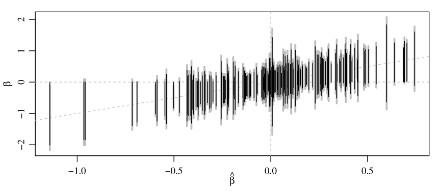
Figure 1: 95% confidence intervals for motif regression effects. UMAU intervals are thick gray lines, FAB intervals are thin black lines.

4.2 Motif regression simulation study

Zhang and Zhang (2014) developed a confidence interval procedure for sparse parameters in high-dimensional normal linear regression models. When applied to the motif dataset, this low dimensional projection (LDP) procedure produces intervals that are narrower than the FAB intervals for all regression coefficients, with relative widths ranging from 0.27 to 0.71, and being about half as wide on average across coefficients. However, unlike the FAB and UMAU procedures, the actual coverage rates of LDP intervals are guaranteed to achieve their nominal rates only asymptotically, and only if certain sparsity conditions on ${\boldsymbol{\beta}}$ are met.

To compare the performance of the UMAU, FAB and LDP procedures we constructed two related simulation studies based on the motif binding dataset described in the previous subsection. In each study, we obtained estimates $({{\boldsymbol{\beta}}}_{0},\sigma^{2}_{0})$ from the real data ${\mathbf{y}}$ and ${\mathbf{X}}$, and used these estimates to simulate new response vectors ${\mathbf{y}}^{(k)}\sim N({\mathbf{X}}{{\boldsymbol{\beta}}}_{0},\sigma^{2}_{0}{\mathbf{I}})$ independently for $k=1,\ldots,5000$. For each response vector ${\mathbf{y}}^{(k)}$ we construct UMAU, FAB and LDP confidence intervals for each of the $p=195$ regression coefficients. These intervals are used to obtain Monte Carlo approximations to the finite-sample coverage rates of the LDP procedure, as well as approximations to the expected interval widths of the UMAU, FAB and LDP procedures.

In the first of these two simulation studies we simulated 5000 datasets from the model ${\mathbf{y}}^{(k)}\sim N_{n}({\mathbf{X}}{\boldsymbol{\beta}}_{0},\sigma^{2}_{0}{\mathbf{I}})$, where ${\mathbf{X}}$ is the original design matrix and ${\boldsymbol{\beta}}_{0}$ is the lasso estimate from the original data, using an empirical Bayes estimate of the $L_{1}$-penalty parameter. This resulted in a sparse ${{\boldsymbol{\beta}}}_{0}$-vector with 176 of the 195 coefficients being identically zero, so in the context of this simulation study, the “truth” is highly sparse. The value of $\sigma^{2}_{0}$ used to simulate the data was the usual unbiased estimate from the original data. We computed the UMAU, FAB and LDP confidence intervals for each of the 5000 simulated datasets. The widths of the FAB and LDP intervals were 85% and 43% of the UMAU interval widths respectively, on average across datasets and parameters. The empirical coverage rates of the nominal 95% LDP intervals ranged between 93.8 and 96.1 percent. There was some evidence that the coverage rates were not exactly 95%: Exact level-.05 binomial tests rejected the hypothesis that the coverage rates were 95% for 71 of the 195 regression parameters (36%). All of these 71 parameters had true values of 0, and the empirical coverage rates of 64 of these 71 parameters were larger than 95%, suggesting that LDP intervals slightly overcover $\beta_{j}$ when it is zero. However, in general the coverage rates of the LDP procedure were very close to the nominal rates, in this case where the truth is sparse.

The second simulation study was the same as the first except the value ${\boldsymbol{\beta}}_{0}$ used to generate the simulated data was the OLS estimate from the original data, and so in this case the “true” regression model is not sparse. On average across the 5000 simulated datasets and 195 parameters, the widths of the FAB and LDP intervals were 88% and 54% of the UMAU interval widths respectively, similar to the results from the first study. These relative widths are shown in the left panel of Figure 2. However, the coverage rates for the LDP intervals were generally far from their nominal levels: Based on exact binomial tests, coverage rates for 183 of the 195 parameters were significantly different from 95% (at level 0.05). As shown in the right panel of Figure 2, the LDP intervals generally overcover parameter values near zero, and greatly undercover parameters larger in magnitude. For comparison, the empirical coverage rates of the FAB intervals are also shown. These rates show no evidence of deviation from the nominal rates, as should be the case - the FAB intervals have exact 95% coverage for each component of ${\boldsymbol{\beta}}$ by construction.

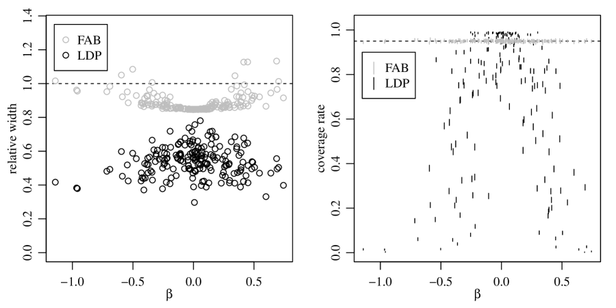
Figure 2: Relative interval widths (left panel) and coverage rates (right panel) for the motif simulation study with non-sparse ${\boldsymbol{\beta}}$. Error bars for the coverage rates are Clopper-Pearson 95% intervals.

4.3 Diabetes progression

Efron et al. (2004) considered parameter estimation for a model of diabetes progression from data on ten explanatory variables from each of $n=442$ subjects. The expected progression of a subject was assumed to be a linear function of the linear, quadratic and two-way interaction effects of the ten variables, resulting in a linear model with $p=64$ regressors total (the binary sex variable does not have a separate quadratic effect).

We generally expect that main effects will be larger than quadratic effects and two-way interactions. For this reason, it makes sense to obtain adaptive intervals separately for these three types of parameters, so that the spending function $\tilde{s}$ used to obtain the confidence interval for the effect of a given regressor is obtained adaptively from the estimated effects of regressors in the same category. This can easily be done as follows: Write the design matrix ${\mathbf{X}}$ as ${\mathbf{X}}=[{\mathbf{X}}_{1},{\mathbf{X}}_{2},{\mathbf{X}}_{3}]$, where ${\mathbf{X}}_{1}$, ${\mathbf{X}}_{2}$, ${\mathbf{X}}_{3}$ are the design matrices corresponding to the main effects, quadratic effects and two-way interactions, respectively, and let ${\boldsymbol{\beta}}^{\top}=[{\boldsymbol{\beta}}^{\top}_{1},{\boldsymbol{\beta}}^{\top}_{2},{\boldsymbol{\beta}}^{\top}_{3}]$ be the corresponding partition of ${\boldsymbol{\beta}}$. To obtain the FAB CIs for the main effects, we let ${\mathbf{G}}$ be an orthonormal basis for the null space of $[{\mathbf{X}}_{2},{\mathbf{X}}_{3}]$. Letting $\tilde{{\mathbf{y}}}={\mathbf{G}}^{\top}{\mathbf{y}}$ and $\tilde{{\mathbf{X}}}={\mathbf{G}}^{\top}{\mathbf{X}}$, we have $\tilde{{\mathbf{y}}}\sim N_{n-p_{2}-p_{3}}(\tilde{{\mathbf{X}}}{\boldsymbol{\beta}}_{1},\sigma^{2}{\mathbf{I}})$. We can then apply the FAB CI procedure to $(\tilde{{\mathbf{y}}},\tilde{{\mathbf{X}}})$ to obtain intervals that adapt to the magnitude of ${\boldsymbol{\beta}}_{1}$ (and not to the magnitudes of ${\boldsymbol{\beta}}_{2}$ and ${\boldsymbol{\beta}}_{3}$). Adaptive confidence intervals for ${\boldsymbol{\beta}}_{2}$ and ${\boldsymbol{\beta}}_{3}$ can be obtained analogously.

In the analysis that follows we use an adaptively estimated $N(0,\tau^{2})$ prior distribution for each coefficient. Recall that our FAB procedure generates an empirical Bayes estimate $\tilde{\tau}^{2}$ of $\tau^{2}={\text{Var}}[\beta_{j}]$ for each coefficient $j$ that is statistically independent of the OLS estimate $\hat{\beta}_{j}$. For the main effects the values of $\tilde{\tau}$ ranged between 0.19 and 0.21, with a mean of 0.20, and were larger than the standard errors of the OLS coefficients except for those of four somewhat co-linear predictors. In contrast, values of $\tilde{\tau}$ for the quadratic and interaction terms were all less than 0.03, and were all less than the corresponding standard errors.

We computed the adaptive FAB interval for each regression coefficient using these coefficient-specific estimates of $\tau^{2}$. The FAB intervals are as narrow or narrower than all but three of the corresponding UMAU intervals, with the relative interval widths ranging from 0.84 to 1.0003, and being 0.86 on average. The FAB CIs for the main effects are essentially the same as the UMAU CIs, whereas the FAB CIs for the quadratic and interaction terms are all narrower than the corresponding UMAU intervals, by about 16% on average. This example illustrates some flexibility of the FAB procedure, in that the adaptation for a particular parameter may be based on a subset of the data information that is deemed most relevant for that parameter.

5 Discussion

We have constructed a class of $1-\alpha$ confidence interval procedures (CIPs) for individual regression coefficients of the normal regression model ${\mathbf{y}}\sim N_{n}({\mathbf{X}}{\boldsymbol{\beta}},\sigma^{2}{\mathbf{I}})$. Each member of this class corresponds to a spending function $s:\mathbb{R}\rightarrow[0,1]$. Under the regression model, every member of the class has constant $1-\alpha$ coverage for all possible values of ${\boldsymbol{\beta}}$, $\sigma^{2}$ and full-rank design matrices ${\mathbf{X}}$. We have described a method of adaptively selecting the spending function so that the across-parameter average interval width is reduced, and the $1-\alpha$ coverage rate is maintained for each regression coefficient. The coverage guarantee is non-asymptotic, does not rely on ${\boldsymbol{\beta}}$ being sparse and does not rely on conditions on the design matrix. However, under some assumptions on the distribution of the elements of ${\boldsymbol{\beta}}$ and the design matrix, the adaptive technique we propose is asymptotically optimal as both $n$ and $p$ increase.

The spending function $s(\beta)$ that we adaptively estimate from the data is based on a normal prior distribution for the elements of ${\boldsymbol{\beta}}$. As such, we expect our procedure to provide the most improvement when the empirical distribution of $\beta_{1},\ldots,\beta_{p}$ is approximately normal. If instead we suspect that ${\boldsymbol{\beta}}$ is sparse, it may seem preferable to base the adaptation on other families of prior distributions, such as Laplace or “spike and slab” distributions. Some numerical work not presented here suggests that FAB intervals obtained using the Laplace family of priors are in practice similar to those obtained with normal priors. However, FAB procedures based on spike and slab priors do seem more efficient but also present a problem: The spending function for a spike and slab prior is not generally nondecreasing, and so by Theorem 1 the corresponding confidence region may not be an interval. We suspect that non-interval confidence regions have limited appeal in practice, but even if they were of interest they present the numerical challenge of identifying multiple disconnected sets of parameter values to include in the region.

We conjecture that the LDP interval procedure proposed by Zhang and Zhang (2014) could be related to a FAB procedure based on a sparsity-inducing prior distribution, as both procedures should be asymptotically optimal under a sparse regime. The fact that a FAB procedure based on such a prior might produce non-interval confidence regions might partly explain why the LDP procedure fails when ${\boldsymbol{\beta}}$ is non-sparse: If a sparse $1-\alpha$ FAB procedure yields a non-interval region but only a sub-interval is numerically identified, then the coverage rate will be below $1-\alpha$.

Adaptive FAB intervals for linear regression coefficients may be computed using the R-package fabCI. Complete replication code for the numerical examples in this article is available at the first author’s website. This research was partially supported by NSF grant DMS-1505136.

Proofs

Proof of Theorem 1

Items 1 and 2 of the theorem were shown in Yu and Hoff (2016). To prove Item 3, suppose $s(\theta)$ is not nondecreasing so that there exists $\theta_{1}<\theta_{2}$ with $s(\theta_{1})>s(\theta_{2})$. We will show that there are a range of values of $(\hat{\theta},\hat{\sigma})$ with $\hat{\theta}<\theta_{1}$ for which $\theta_{2}$ (and $\hat{\theta}$) are in $C_{s}(\hat{\theta},\hat{\sigma})$ but $\theta_{1}$ is not. Let $\underline{t}_{j}=t_{\alpha(1-s(\theta_{j}))}$ and $\bar{t}_{j}=t_{1-\alpha s(\theta_{j})}$ for $j=1,2$. Both $t_{\alpha(1-s)}$ and $t_{1-\alpha s}$ are decreasing in $s$ so $\underline{t}_{1}<\underline{t}_{2}<\bar{t}_{1}<\bar{t}_{2}$. For $\theta_{2}$ to be in the confidence region and $\theta_{1}$ not to be, we need $\hat{\theta}+\hat{\sigma}\underline{t}_{2}<\theta_{2}<\hat{\theta}+\hat{\sigma}\bar{t}_{2}$ and $\theta_{1}>\hat{\theta}+\hat{\sigma}\bar{t}_{1}$, or equivalently

$$\bar{t}_{1} <(\theta_{1}-\hat{\theta})/\hat{\sigma}$$ (10)

$$\underline{t}_{2} <(\theta_{2}-\hat{\theta})/\hat{\sigma}<\bar{t}_{2}.$$ (11)

The set of values $(\hat{\theta},\hat{\sigma})$ for which this holds has positive Lebesgue measure on $(-\infty,\theta_{1})\times(0,\infty)$. For example, both $(\theta_{1}-\hat{\theta})/\hat{\sigma}$ and $(\theta_{2}-\hat{\theta})/\hat{\sigma}$ can be made simultaneously arbitrarily close to any number between $\bar{t}_{1}\wedge\underline{t}_{2}$ and $\bar{t}_{2}$ by taking $\hat{\sigma}$ and $-\hat{\theta}$ to be sufficiently large. The probability of observing values of $(\hat{\theta},\hat{\sigma})$ satisfying (10) and (11) that yield a non-interval confidence region is therefore greater than zero.

Proof of Lemma 1

For notational convenience, in this proof we write $\beta_{j}$ and $w_{j}$ as $\beta$ and $w$, and write the $\alpha$-quantile of the $t_{q}$ distribution as $t(\alpha)$, suppressing the index that denotes the degrees of freedom. We begin the proof of Lemma 2 with another lemma:

Lemma 3.

The width $|C_{\tilde{s}}|$ of $C_{\tilde{s}}$ satisfies $|C_{\tilde{s}}|<|\hat{\beta}|+w\hat{\sigma}(|t(\alpha/2)|+|t(1-\alpha/2)|)$.

Proof.

Recall that the endpoints $\underline{\beta}$ and $\bar{\beta}$ of $C_{\tilde{s}}$ are solutions to

$$\hat{\beta} =\bar{\beta}-w\hat{\sigma}t(1-\alpha\tilde{s}(\bar{\beta}))$$

$$\hat{\beta} =\underline{\beta}-w\hat{\sigma}t(\alpha(1-\tilde{s}(\underline{\beta})))$$

Here $\tilde{s}(\beta)$ is defined as $\tilde{s}(\beta)=g^{-1}(2w\tilde{\sigma}\beta/{\tilde{\tau}}^{2})$, where $g(s)=\Phi^{-1}(\alpha s)-\Phi^{-1}(\alpha(1-s))$. At the upper endpoint, we have $\tilde{s}(\bar{\beta})=F((\hat{\beta}-\bar{\beta})/(w\hat{\sigma}))/\alpha$, where $F$ is the CDF of the $t_{q}$-distribution. When $\bar{\beta}>0$, we have $\tilde{s}(\bar{\beta})>g^{-1}(0)=1/2$. Thus $\bar{\beta}<\hat{\beta}-w\hat{\sigma}t(\alpha/2)$. Also, $g^{-1}(2w\tilde{\sigma}\bar{\beta}/{\tilde{\tau}}^{2})<1$, so $\bar{\beta}>\hat{\beta}-w\hat{\sigma}t(\alpha)$. When $\bar{\beta}<0$, $\hat{\beta}-w\hat{\sigma}t(\alpha/2)<\bar{\beta}$. This implies that

$$\hat{\beta}-w\hat{\sigma}t(\alpha)<\bar{\beta}<\hat{\beta}-w\hat{\sigma}t(\alpha/2) \ \text{if}\ \bar{\beta}>0$$

$$\hat{\beta}-w\hat{\sigma}t(\alpha/2)<\bar{\beta}<0 \ \text{if}\ \bar{\beta}<0.$$

Similarly we have

$$0<\underline{\beta}<\hat{\beta}-w\hat{\sigma}t(1-\alpha/2) \ \text{if}\ \underline{\beta}>0$$

$$\hat{\beta}-w\hat{\sigma}t(1-\alpha/2)<\underline{\beta}<\hat{\beta}-w\hat{\sigma}t(1-\alpha) \ \text{if}\ \underline{\beta}<0.$$

Therefore

$$|C_{\tilde{s}}|=\bar{\beta}-\underline{\beta}<|\hat{\beta}|+w\hat{\sigma}(|t(\alpha/2)|+|t(1-\alpha/2)|).$$

∎

Now we prove Lemma 1. We denote the endpoints of the oracle CIP $C_{s}$ as $\bar{\beta}$ and $\underline{\beta}$, which are the solutions to

$$\begin{array}[]{l}\bar{\beta}-w_{0}\sigma_{\infty}\Phi^{-1}(1-\alpha s(\bar{\beta}))=\hat{\beta}\\ \underline{\beta}-w_{0}\sigma_{\infty}\Phi^{-1}(\alpha(1-s(\underline{\beta})))=\hat{\beta}.\\ \end{array}$$

We denote the endpoints of $C_{\tilde{s}}$ as $\bar{\beta}^{n}$ and $\underline{\beta}^{n}$, which are the solutions to

$$\begin{array}[]{l}\bar{\beta}^{n}-w\hat{\sigma}t(1-\alpha\tilde{s}(\bar{\beta}^{n}))=\hat{\beta}^{n}\\ \underline{\beta}^{n}-w\hat{\sigma}t(\alpha(1-\tilde{s}(\underline{\beta}^{n})))=\hat{\beta}^{n}.\\ \end{array}$$

We first prove that $|C_{\tilde{s}}|-|C_{s}|=(\bar{\beta}^{n}-\bar{\beta})+(\underline{\beta}-\underline{\beta}^{n})\stackrel{{\scriptstyle p}}{{\rightarrow}}0$ as $n\to\infty$ for each fixed $\hat{\beta}$. We can write the upper endpoints as $\bar{\beta}^{n}=G_{n}(w\hat{\sigma},w\tilde{\sigma},\tilde{\tau}^{2},\hat{\beta}^{n})$, and $\bar{\beta}=G(w_{0}\sigma_{\infty},w_{0}\sigma_{\infty},\tau^{2},\hat{\beta})$, where $G$ and $G_{n}$ are continuous functions of their parameters. The functions $G$ and $G_{n}$ are different in that the former is based on $z$-quantiles, while the latter uses $t$-quantiles. We have

$$\begin{split}|\bar{\beta}^{n}-\bar{\beta}|&=|G_{n}(w\hat{\sigma},w\tilde{\sigma},\tilde{\tau}^{2},\hat{\beta}^{n})-G(w_{0}\sigma_{\infty},w_{0}\sigma_{\infty},\tau^{2},\hat{\beta})|\\ &\leq|G_{n}(w\hat{\sigma},w\tilde{\sigma},\tilde{\tau}^{2},\hat{\beta}^{n})-G(w\hat{\sigma},w\tilde{\sigma},\tilde{\tau}^{2},\hat{\beta}^{n})|\\ &+|G(w\hat{\sigma},w\tilde{\sigma},\tilde{\tau}^{2},\hat{\beta}^{n})-G(w_{0}\sigma_{\infty},w_{0}\sigma_{\infty},\tau^{2},\hat{\beta})|.\end{split}$$ (12)

The second term converges to zero in probability because $(w\hat{\sigma},w\tilde{\sigma},\tilde{\tau}^{2},\hat{\beta}^{n})\stackrel{{\scriptstyle p}}{{\rightarrow}}(w_{0}\sigma_{\infty},w_{0}\sigma_{\infty},\tau^{2},\hat{\beta})$. Elaborating on the convergence of the first term, note that $G_{n}$ is a monotone sequence of continuous functions: Given $G_{n1}$ and $G_{n2}$ where $n_{2}>n_{1}$, and suppose the corresponding degrees-of-freedom of the $t$-quantiles are $q_{1}$ and $q_{2}$. We have $q_{2}\geq q_{1}$, thus $t_{q_{2}}(1-\alpha\tilde{s})\leq t_{q_{1}}(1-\alpha\tilde{s})$. Hence $\hat{\beta}^{n}-w\hat{\sigma}t_{q_{2}}(1-\alpha\tilde{s}(\hat{\beta}^{n}))\geq\hat{\beta}^{n}-w\hat{\sigma}t_{q_{1}}(1-\alpha\tilde{s}(\hat{\beta}^{n}))$. Therefore $G_{q_{2}}(w\hat{\sigma}^{2},w\tilde{\sigma}^{2},\tilde{\tau}^{2},\hat{\beta}^{n})\leq G_{q_{1}}(w\hat{\sigma}^{2},w\tilde{\sigma}^{2},\tilde{\tau}^{2},\hat{\beta}^{n})$, and so by Dini’s theorem, $G_{n}\rightarrow G$ uniformly on a compact set of $(s^{2}\hat{\sigma}^{2},s^{2}\tilde{\sigma}^{2},\tilde{\tau}^{2},\hat{\beta}^{n})$ values. Since $(s^{2}\hat{\sigma}^{2},s^{2}\tilde{\sigma}^{2},\tilde{\tau}^{2},\hat{\beta}^{n})\stackrel{{\scriptstyle p}}{{\rightarrow}}(v^{2}\sigma_{\infty}^{2},v^{2}\sigma_{\infty}^{2},\tau^{2},\hat{\beta})$, for arbitrary $\epsilon>0$ and $\delta>0$, there exists a number $N(\epsilon,\delta)$ such that when $n>N(\epsilon,\delta)$, $|w\hat{\sigma}-w_{0}\sigma_{\infty}|\leq\delta$, $|w\tilde{\sigma}-w_{0}\sigma_{\infty}|\leq\delta$, $|\tilde{\tau}^{2}-\tau^{2}|\leq\delta$ and $|\hat{\beta}^{n}-\hat{\beta}|\leq\delta$ with probability at least $1-\epsilon$. Therefore, for arbitrary $\eta>0$,

$$\lim_{n\to\infty}P(|G_{n}(w\hat{\sigma},w\tilde{\sigma},\tilde{\tau}^{2},\hat{\beta}^{n})-G(w\hat{\sigma},w\tilde{\sigma},\tilde{\tau}^{2},\hat{\beta})|<\eta)>1-\epsilon.$$

Since $\epsilon$ is arbitrary, we conclude that the first term in (12) converges to zero in probability.

Now we show the expected width converges to the oracle width by integrating over $\hat{\beta}$. This is done by first showing $|C_{\tilde{s}}|$ is uniformly integrable and then applying Vitali’s theorem. By the previous lemma we know that

$$|C_{\tilde{s}}|<|\hat{\beta}^{n}|+w\hat{\sigma}(|t(\alpha/2)|+|t(1-\alpha/2)|).$$

Note that $|t(\alpha/2)|+|t(1-\alpha/2)|<|t_{1}(\alpha/2)|+|t_{1}(1-\alpha/2)|=c_{1}<\infty$, where $t_{1}$ is the $t$-quantile with one degree of freedom. We now show $|C_{\tilde{s}}|$ is $L_{2}$-bounded. We have

$$|C_{\tilde{s}}|^{2}<|\hat{\beta}^{n}|^{2}+c_{1}^{2}w^{2}\hat{\sigma}^{2}+2|\hat{\beta}^{n}|c_{1}w\hat{\sigma}.$$

Here $E[|\hat{\beta}^{n}|^{2}]=\beta^{2}+w^{2}\sigma^{2}$ and $E[w^{2}\hat{\sigma}^{2}]=w^{2}\sigma^{2}$. Since $w^{2}\sigma^{2}\to w_{0}^{2}\sigma_{\infty}^{2}<\infty$, thus $E[|\hat{\beta}^{n}|^{2}]$ and $E[w^{2}\hat{\sigma}^{2}]$ are both bounded for all $n$. Similarly, $E[w\hat{\sigma}]$ and $E[|\hat{\beta}^{n}|]$ are also bounded. Therefore, it is easy to see that $|C_{\tilde{s}}|$ is $L_{2}$-bounded, which implies that $|C_{\tilde{s}}|$ is uniformly integrable. By Vitali’s Theorem, $\lim_{n\rightarrow\infty}{\text{E}}[|C_{\tilde{s}}|]={\text{E}}[|C_{s}|]=0$.

Proof of Lemma 2

We first prove a consistency result for a notationally simpler model, and then discuss how the result applies to the marginal model (9). The simpler model is ${\mathbf{y}}\sim N_{n}({\mathbf{0}},\Lambda\tau^{2}+{\mathbf{I}}\sigma^{2})$ where $\Lambda$ is a known diagonal matrix with positive entries. Let $\theta_{0}=(\tau^{2}_{0},\sigma^{2}_{0})$ be the true value of $\theta=(\tau^{2},\sigma^{2})$, and let $q_{i}(\theta)=y_{i}^{2}/(\lambda_{i}\tau^{2}+\sigma^{2})-\log\frac{\lambda_{i}\tau^{2}_{0}+\sigma^{2}_{0}}{\lambda_{i}\tau^{2}+\sigma^{2}}$, which is -2 times the contribution of $y_{i}$ to the log likelihood plus a constant. The MLE is therefore given by $\hat{\theta}=\arg\min Q_{n}(\theta)$, where $Q_{n}(\theta)=\sum_{i=1}^{n}q_{i}(\theta)/n$.

Lemma 4.

Assume $\theta_{0}\in\Theta$, a compact subset of $[0,\infty)\times(0,\infty)$, and let $\hat{\theta}_{n}=\arg\min_{\Theta}Q_{n}(\theta)$. For each $n$ assume that $F_{n}$, the empirical distribution of the diagonal entries of $\Lambda$, has support on $[0,\bar{\lambda}]$, where $\bar{\lambda}$ is fixed for all $n$. If $F_{n}$ converges weakly to a nondegenerate distribution $F_{0}$ as $n\rightarrow\infty$ then $\hat{\theta}\stackrel{{\scriptstyle p}}{{\rightarrow}}\theta_{0}$ as $n\rightarrow\infty$.

We prove consistency of $\hat{\theta}$ in three steps: First, we show that $Q_{n}(\theta)-{\text{E}}[Q_{n}(\theta)]$ converges uniformly to zero as $n\rightarrow\infty$. Second, we show that this implies that as a function of $\theta\in\Theta$, $Q_{n}$ converges uniformly to a function $Q_{0}$. Third, we show that $Q_{0}$ is uniquely minimized at $\theta_{0}$. Consistency of $\hat{\theta}$ follows from these latter two results (see, for example, Theorem 2.1 of Newey and McFadden (1994)).

For each $n$ the expectation of $Q_{n}(\theta)-{\text{E}}[Q_{n}(\theta)]$ is zero and the variance is given by

$${\text{Var}}[Q_{n}(\theta)]=\frac{2}{n}\left(\frac{1}{n}\sum_{i=1}^{n}(\frac{\lambda_{i}\tau^{2}_{0}+\sigma^{2}_{0}}{\lambda_{i}\tau^{2}+\sigma^{2}})^{2}\right)=\frac{2}{n}\left(\int(\frac{\lambda\tau^{2}_{0}+\sigma^{2}_{0}}{\lambda\tau^{2}+\sigma^{2}})^{2}\,dF_{n}(\lambda)\right).$$

The integrand is a bounded function of $\lambda$ on any bounded set $[0,\bar{\lambda}]$ as long as $\sigma^{2}>0$. Therefore, if $F_{n}$ converges weakly to a distribution $F_{0}$ with such bounded support, then for all $\theta=(\tau^{2},\sigma^{2})\in[0,\infty)\times(0,\infty)$ the integral in the parentheses converges to a finite limit and the variance of $Q_{n}(\theta)-{\text{E}}[Q_{n}(\theta)]$ converges to zero. Thus $Q_{n}(\theta)-{\text{E}}[Q_{n}(\theta)]\stackrel{{\scriptstyle p}}{{\rightarrow}}0$ as $n\rightarrow\infty$. To show that this convergence is uniform we use Theorem 3 of Andrews (1992). Using basic calculus, it can be shown that the functions $q_{i}(\theta)$ satisfy the Lipschitz condition $|q_{i}(\theta)-q_{i}(\theta^{\prime})|<g(y_{i},\lambda_{i})\times||\theta-\theta^{\prime}||$ where $g(y_{i},\lambda_{i})=(1+y_{i}^{2}/\epsilon)(\lambda_{i}+1)/\epsilon$ and $\epsilon=\min_{\Theta}\sigma^{2}$. Andrews’ Theorem 5 says that if (i) $\Theta$ is compact, (ii) $Q_{n}\stackrel{{\scriptstyle p}}{{\rightarrow}}0$ for each $\theta\in\Theta$, and (iii) $\sup_{n\geq 1}\sum{\text{E}}[g(y_{i},\lambda_{i})]/n<\infty$, then $\sup_{\Theta}|Q_{n}(\theta)|\stackrel{{\scriptstyle p}}{{\rightarrow}}0$. This last condition holds in this case because ${\text{E}}[g(y_{i},\lambda_{i})]$ is quadratic in $\lambda_{i}$, the values of which are all bounded by assumption. Therefore, $Q_{n}(\theta)$ converges uniformly in probability to zero as $n\rightarrow\infty$.

Now consider the limiting value of ${\text{E}}[Q_{n}(\theta)]$. We have

$$\lim_{n\rightarrow\infty}{\text{E}}[Q_{n}(\theta)] =\lim_{n\rightarrow\infty}\int\left(\frac{\lambda\tau_{0}^{2}+\sigma_{0}^{2}}{\lambda\tau^{2}+\sigma^{2}}-\log\frac{\lambda\tau_{0}^{2}+\sigma_{0}^{2}}{\lambda\tau^{2}+\sigma^{2}}\right)\,dF_{n}(\lambda)$$

$$=\int\left(\frac{\lambda\tau_{0}^{2}+\sigma_{0}^{2}}{\lambda\tau^{2}+\sigma^{2}}-\log\frac{\lambda\tau_{0}^{2}+\sigma_{0}^{2}}{\lambda\tau^{2}+\sigma^{2}}\right)\,dF_{0}(\lambda)\equiv Q_{0}(\theta),$$

for all values of $\theta$ for which the integrand is a bounded function of $\lambda$. On $\lambda\in[0,\bar{\lambda}]$, the ratio $(\lambda\tau^{2}_{0}+\sigma_{0}^{2})/(\lambda\tau^{2}+\sigma^{2})$ is bounded between $\min\{\tfrac{\bar{\lambda}\tau^{2}_{0}+\sigma_{0}^{2}}{\bar{\lambda}\tau^{2}+\sigma^{2}},\tfrac{\sigma^{2}_{0}}{\sigma^{2}}\}$ and $\max\{\tfrac{\bar{\lambda}\tau^{2}_{0}+\sigma_{0}^{2}}{\bar{\lambda}\tau^{2}+\sigma^{2}},\tfrac{\sigma^{2}_{0}}{\sigma^{2}}\}$, and so the integrand is bounded in $\lambda\in[0,\bar{\lambda}]$ for all $(\tau^{2},\sigma^{2})\in[0,\infty)\times(0,\infty)$. Furthermore, the convergence of ${\text{E}}[Q_{n}(\theta)]$ to $Q_{0}(\theta)$ is uniform, since the integrand is bounded as a function of $\theta$ on the compact set $\Theta$ (Ranga Rao (1962)). Together with the uniform convergence in probability of $Q_{n}(\theta)-{\text{E}}[Q_{n}(\theta)]$ to zero, this implies uniform convergence in probability of $Q_{n}$ to $Q_{0}$.

Finally we show that $Q_{0}(\theta)$ has a unique minimizing value at $\theta_{0}$. After computing the gradient of $Q_{0}(\theta)$, it is easily shown that a critical point $(\tau^{2},\sigma^{2})$ must satisfy

$$\int\lambda^{k}\frac{\lambda\tau^{2}+\sigma^{2}}{(\lambda\tau^{2}+\sigma^{2})^{2}}\,dF_{0}(\lambda)=\int\lambda^{k}\frac{\lambda\tau^{2}_{0}+\sigma^{2}_{0}}{(\lambda\tau^{2}+\sigma^{2})^{2}}\,dF_{0}(\lambda)$$

for $k\in\{0,1\}$. Rearranging, it can be shown that a critical point satisfies

$$\begin{pmatrix}m_{1}&1\\ m_{2}&m_{1}\end{pmatrix}\begin{pmatrix}\tau^{2}\\ \sigma^{2}\end{pmatrix}=\begin{pmatrix}m_{1}&1\\ m_{2}&m_{1}\end{pmatrix}\begin{pmatrix}\tau^{2}_{0}\\ \sigma^{2}_{0}\end{pmatrix}$$ (13)

where $m_{k}(\tau^{2},\sigma^{2})$, $k\in\{1,2\}$ is given by

$$m_{k}(\tau^{2},\sigma^{2})=\frac{\int\lambda^{k}(\lambda\tau^{2}+\sigma^{2})^{-2}\,dF_{0}(\lambda)}{\int(\lambda\tau^{2}+\sigma^{2})^{-2}\,dF_{0}(\lambda)}.$$

For each $(\tau^{2},\sigma^{2})\in[0,1)\times(0,\infty)$, $m_{1}$ and $m_{2}$ are the first and second moments of $\lambda$ under a probability measure having density with respect to $F_{0}$ proportional to $(\lambda\tau^{2}+\sigma^{2})^{-2}$. If $F_{0}$ is not degenerate, then $m_{2}>m_{1}^{2}$, and so the determinant of the matrix in (13) is non-zero. Therefore, the matrix is invertible and $(\tau^{2}_{0},\sigma_{0}^{2})$ is the only solution to (13). The matrix of second derivatives of $Q_{0}$ is given by

$$\frac{\partial^{2}Q_{0}}{\partial\theta\partial\theta^{\top}}=\int\begin{pmatrix}\lambda^{2}&\lambda\\ \lambda&1\end{pmatrix}\frac{2(\lambda\tau^{2}_{0}+\sigma^{2}_{0})-(\lambda\tau^{2}+\sigma^{2})}{\lambda\tau^{2}+\sigma^{2}}\times(\lambda\tau^{2}+\sigma^{2})^{-2}\,dF_{0}(\lambda).$$

At the critical point $(\tau^{2}_{0},\sigma^{2}_{0})$ this simplifies to the expectation of the matrix in the integrand with respect to the probability measure with density proportional to $(\lambda\tau^{2}+\sigma^{2})^{-2}$ with respect to $F_{0}$. Again, if $F_{0}$ is not degenerate then the expectation of this matrix, and hence the Hessian of $Q_{0}$, is strictly positive definite. The critical point is a local minimum, and since it is the only critical point of the continuous function $Q_{0}$, it is the unique minimizer. This completes the proof of Lemma 4.

To see how this applies to the properties of the empirical Bayes estimates $(\tilde{\tau}^{2},\tilde{\sigma}^{2})$ of $(\tau^{2},\sigma^{2})$ based on the marginal model (9), let ${\mathbf{U}}$ be the $(p-1)\times(p-1)$ matrix of left singular vectors of ${\mathbf{X}}_{2}$, and let $n{\boldsymbol{\Lambda}}_{2}$ be the diagonal matrix of the squared singular values. Then ${\mathbf{U}}_{2}^{\top}{\mathbf{z}}_{2}/\sqrt{n}\sim N_{p-1}({\mathbf{0}},{\boldsymbol{\Lambda}}_{2}\tau^{2}+{\mathbf{I}}\sigma_{\infty}^{2})$, and so the properties of the MLE of $(\tau^{2},\sigma^{2}_{\infty})$ based on ${\mathbf{z}}_{2}$ will be the same as those of $(\tau^{2},\sigma^{2})$ in Lemma 4 if ${\boldsymbol{\Lambda}}_{2}$ satisfies the assumption of the Lemma. To see that it does, recall that the assumption of Lemma 2 was that the empirical distribution of the eigenvalues of ${\mathbf{X}}^{\top}{\mathbf{X}}/n$ is uniformly bounded and converges weakly to a non-degenerate distribution with finite support. For a given $n$, let $\gamma_{1},\ldots,\gamma_{p}$ be the eigenvalues of ${\mathbf{X}}^{\top}{\mathbf{X}}/n$. Since ${\mathbf{X}}_{2}^{\top}{\mathbf{X}}_{2}/n$ is a compression of ${\mathbf{X}}^{\top}{\mathbf{X}}/n$, by the Cauchy interlacing theorem we have $\gamma_{1}\leq\lambda_{1}\leq\gamma_{2}\leq\cdots\leq\gamma_{p-1}\leq\lambda_{p-1}\leq\gamma_{p}$. Therefore, if the values of $\{\gamma_{1},\ldots,\gamma_{p}\}$ are bounded uniformly in $p$ and have an empirical distribution that converges to a nondegenerate limit, then the same properties hold for the values of $\{\lambda_{1},\ldots,\lambda_{p-1}\}$.

References

• Andrews (1992) Andrews, D. W.ย K. (1992). Generic uniform convergence. Econometric Theoryย 8(2), 241โ€“257.
• Bรผhlmann (2013) Bรผhlmann, P. (2013). Statistical significance in high-dimensional linear models. Bernoulliย 19(4), 1212โ€“1242.
• Conlon etย al. (2003) Conlon, E.ย M., X.ย S. Liu, J.ย D. Lieb, and J.ย S. Liu (2003). Integrating regulatory motif discovery and genome-wide expression analysis. Proceedings of the National Academy of Sciencesย 100(6), 3339โ€“3344.
• Efron etย al. (2004) Efron, B., T.ย Hastie, I.ย Johnstone, and R.ย Tibshirani (2004). Least angle regression. Ann. Statist.ย 32(2), 407โ€“499. With discussion, and a rejoinder by the authors.
• Kabaila and Tissera (2014) Kabaila, P. and D.ย Tissera (2014). Confidence intervals in regression that utilize uncertain prior information about a vector parameter. Australian & New Zealand Journal of Statisticsย 56(4), 371โ€“383.
• Lee etย al. (2016) Lee, J.ย D., D.ย L. Sun, Y.ย Sun, and J.ย E. Taylor (2016). Exact post-selection inference, with application to the lasso. Ann. Statist.ย 44(3), 907โ€“927.
• Meinshausen etย al. (2009) Meinshausen, N., L.ย Meier, and P.ย Bรผhlmann (2009). $p$-values for high-dimensional regression. J. Amer. Statist. Assoc.ย 104(488), 1671โ€“1681.
• Newey and McFadden (1994) Newey, W.ย K. and D.ย McFadden (1994). Large sample estimation and hypothesis testing. In Handbook of econometrics, Vol.ย IV, Volumeย 2 of Handbooks in Econom., pp.ย  2111โ€“2245. North-Holland, Amsterdam.
• Oโ€™Gorman (2001) Oโ€™Gorman, T.ย W. (2001). Using adaptive weighted least squares to reduce the lengths of confidence intervals. Canad. J. Statist.ย 29(3), 459โ€“471.
• Pratt (1963) Pratt, J.ย W. (1963). Shorter confidence intervals for the mean of a normal distribution with known variance. The Annals of Mathematical Statisticsย 34(2), 574โ€“586.
• Rangaย Rao (1962) Rangaย Rao, R. (1962). Relations between weak and uniform convergence of measures with applications. Ann. Math. Statist.ย 33, 659โ€“680.
• vanย de Geer etย al. (2014) vanย de Geer, S., P.ย Bรผhlmann, Y.ย Ritov, and R.ย Dezeure (2014). On asymptotically optimal confidence regions and tests for high-dimensional models. Ann. Statist.ย 42(3), 1166โ€“1202.
• Yu and Hoff (2016) Yu, C. and P.ย Hoff (2016). Adaptive multigroup confidence intervals with constant coverage.
• Zhang and Zhang (2014) Zhang, C.-H. and S.ย S. Zhang (2014). Confidence intervals for low dimensional parameters in high dimensional linear models. J. R. Stat. Soc. Ser. B. Stat. Methodol.ย 76(1), 217โ€“242.