Inhomogeneity growth in two-component fermionic systems

Abstract

The dynamics of fermionic many-body systems is investigated in the framework of Boltzmann-Langevin (BL) stochastic one-body approaches. Within the recently introduced BLOB model, we examine the interplay between mean-field effects and two-body correlations, of stochastic nature, for nuclear matter at moderate temperature and in several density conditions, corresponding to stable or mechanically unstable situations. Numerical results are compared to analytic expectations for the fluctuation amplitude of isoscalar and isovector densities, probing the link to the properties of the employed effective interaction, namely symmetry energy (for isovector modes) and incompressibility (for isoscalar modes). For unstable systems, clusterization is observed. The associated features are compared to analytical results for the typical length and time scales characterizing the growth of unstable modes in nuclear matter and for the isotopic variance of the emerging fragments. We show that the BLOB model is generally better suited than simplified approaches previously introduced to solve the BL equation, and it is therefore more advantageous in applications to open systems, like heavy ion collisions.

I Introduction

The dynamics of many-body interacting systems is a long-standing investigation embracing various domains at the boundary between collective and chaotic processes.

From a one-body modelling perspective, the dynamics of fermionic systems Ring1980 ; Maruhn2010 is efficiently described with the time-dependent Hartree-Fock (TDHF) framework, or time-dependent local density approximation (TDLDA), in condense-matter applications Yabana1999 ; Reinhard2004 , as far as the variance of the involved observables is small and can be neglected. If this is not the case, additional beyond mean-field correlations should be included, depending on the degree of excitation Abe1996 ; Chomaz2004 ; Simenel2010 . At low energy, as far as the system can be described in the small-amplitude limit, a scheme of coherent-state propagation within the time-dependent generator coordinate method (TDGCM) Reinhard1987 ; Goutte2005 , or a variational approach à la Balian-Vénéroni Balian1981 ; Simenel2012 is well suited. On the contrary, when the system experiences a violent dynamics, large fluctuations would spontaneously drive the system far away from the one-body TDHF evolution along many different directions, thus determining the shortcoming of the TDHF approximation (and the above mentioned extensions). To address large-amplitude regimes, solutions beyond the single-particle picture may be needed, for instance by propagating non-correlated states Lacroix2015 . When even the low-energy regime is exceeded, dissipative behaviour results also from in-medium collisions, which are no more hindered by Pauli blocking.

In presence of mean-field instabilities, the collective dynamics may be driven to a chaotic regime; in a nuclear system, this would result in a highly non-linear process, leading to clusterisation from one-body density fluctuations, and oscillation of the neutron and proton fraction. The splitting of a composite system into fragments under violent perturbations signs the occurrence of the most catastrophic effect produced by large-amplitude fluctuations of the neutron and proton content. Such phenomenology, which is common in heavy-ion collisions at Fermi energies EPJAtopicalWCI2006 ; EPJAtopicalNSE2014 , also characterises other fields, like solid-state physics (examples are metal clusters Calvayrac2000 ; Fennel2010 or electrons in nanosystems Chen2005 ), ultracold atomic gases Dalibard1998 ; Bloch2008 or some areas of astrophysics Horowitz2006 ; Sebille2011 ; Schneider2013 ; Burrello2016 . The description of the fragmentation process can only be afforded within approaches beyond the mean-field approximation, incorporating the effect of many-body correlations, which induce fluctuations in the evolution of the one-body density. Adapted to such situation, stochastic approaches typically propagate a bunch of mean-field trajectories within various orders of approximations, like stochastic TDHF (STDHF) formulations Reinhard1992 ; Suraud2014 ; Slama2015 ; Lacombe2016 , or analogue semiclassical schemes within the Boltzmann-Langevin (BL) transport equation Ayik1988 ; Reinhard1992bis .

In the following we exploit the last mentioned BL approach in the form of the recently introduced Boltzmann-Langevin one body (BLOB) model Napolitani2013 ; Rizzo2008 to undertake an exhaustive analysis of the interplay between mean-field and many-body correlations in nuclear matter. We focus thereafter on crucial modelling issues, looking in particular at the dynamics of fluctuations, both in stable systems and in unstable conditions, leading to the disassembly of the system. The purpose is to examine virtues and limits of the BLOB approach, where the BL equation is solved in full phase space, and of corresponding approximations by carrying out a quantitative study of fluctuation amplitudes, and comparing with some analytic expectations which characterise Fermi liquids. This analysis is important also in the spirit of preparing reliable applications to heavy-ion collisions. Indeed a good reproduction of the fluctuation dynamics is crucial for the predictions of features, such as size and isotopic variances, of the products formed in nuclear reactions and to probe their link to the properties of the nuclear effective interaction.

In Sec. II we survey some basic steps leading from a stochastic beyond-mean-field framework to the BLOB method, and related approximations. In Sec. III the dynamics of fluctuations of the one-body density, as given by the linearized BL equation, is discussed for nuclear matter initialized at moderate temperature and in several density conditions. Owing to the presence of two components (neutrons and protons), one observes isovector fluctuation modes, where neutrons and protons oscillate out of phase, and isoscalar modes, with neutrons and protons moving together. Isovector fluctuations are of stable nature, reflecting the properties of the nuclear effective interaction in the isovector channel. The performance of the BLOB model in reproducing analytic expectations for the isovector variance and, in particular, its link to the nuclear symmetry energy is discussed in Sec. IV. For nuclear matter at suitable density and temperature conditions, isoscalar fluctuations may become unstable, yielding a growth of the (isoscalar) fluctuation variance, which triggers a process of clusterisation. Such situation is tested in Sec. V. In the spirit of connecting nuclear matter to open systems, sec. VI explores fluctuation observables related to blobs of matter, which correspond to emerging fragments in open systems. Conclusive statements from reviewing the results form Sec. VII.

II Theoretical survey

II.1 N-body correlations in a stochastic one-body framework in dissipative regimes

It is usual to describe the evolution of an $N$-body system by replacing the Liouville-von Neumann equation with the equivalent BBGKY hierarchy which, for a two-body interaction $V_{ij}$, yields the following chain of coupled equations

$$i\hbar\frac{\partial\rho_{1}}{\partial t} = [k_{1},\rho_{1}]+\textrm{Tr}_{2}[V_{12},\rho_{12}]$$

$$i\hbar\frac{\partial\rho_{12}}{\partial t} = [k_{1}+k_{2}+V_{12},\rho_{12}]+\textrm{Tr}_{3}[V_{13}+V_{23},\rho_{123}]$$

$$\dots$$

$$i\hbar\frac{\partial\rho_{1^{\dots}k}}{\partial t} = \sum_{i=1}^{k}\Big{[}k_{i}+\sum_{j<i}^{k}V_{ij},\rho_{1^{\dots}k}\Big{]}$$

$$+ \sum_{i=1}^{k}\textrm{Tr}_{k+1}[V_{ik\!+\!1},\rho_{1^{\dots}k\!+\!1}]$$

$$\dots$$ , (1)

where $\textrm{Tr}_{k}$ is a partial trace involving the many-body density matrix $\rho_{1^{\dots}k}$ (compact notation where the order corresponds to the number of indexes) and $k_{i}$ are kinetic energy operators. This is the avenue for constructing beyond-mean-field approximations, obtained through custom truncations of the hierarchy, or by reducing the complexity of the involved contributions at given orders. For instance, the inclusion of interactions beyond two bodies would be necessary to account for additional nuclear-structure features Schuck2016 , or cluster correlations, and the explicit inclusion of correlations beyond the order $k=2$ would be necessary to describe high-coupling regimes Lacroix2014 .

If, on the other hand, a suited stochastic approach is adopted, simplified higher-order contributions can be introduced even though not explicitly implemented. Already in a first-order-truncation scheme ($k\!=\!1$) in a low-energy framework, it was found that a stochastic approach can be used to restore all the BBGKY missing orders approximately Lacroix2016 , and generate large-amplitude fluctuations; in this case, a coherent ensemble of mean-field states is propagated along different trajectories from an initial stochastic distribution. Such scheme is however insufficient for our purpose, which is addressing dissipative regimes. In this case, it is necessary to introduce in-medium collisions in a second-order scheme ($k\!=\!2$), explicitly, i.e. the first two lines of the set (1), from which kinetic equations are obtained Balescu1976 ; Balian1991 ; Cassing1992 ; Bonasera1994 . If structure effects are neglected, it is then possible to propagate an incoherent ensemble of mean-field states, supplemented by a fluctuating term, in order to obtain a highly non-linear character of the dynamics. The stochastic treatment is not obtained from exploiting a distribution of initial states but, progressing from a single initial state. It acts intermittently all along the temporal evolution, producing successive splits of a given mean-field trajectory $\rho_{1}$ into subensembles $\rho_{1}^{(n)}$:

$$\rho_{1}\longrightarrow\{\rho_{1}^{(n)};n=1,\dots,\textrm{subens.}\}\;.$$ (2)

This pattern then repeats for each element of the subensemble $\rho_{1}^{(n)}$ till eventually yielding trajectories ordered in bifurcating bundles, each one exhibiting a small variance around the mean trajectory of the corresponding envelope. In particular, in the time interval between two successive splits, when fluctuations are built up, the system propagates keeping the mean trajectory unchanged within each envelope. Thus this time, $\tau$, has to be shorter than the time scales associated with the global effect of the collision integral and with the mean-field propagation.

II.2 Collisional correlations

This stochastic scheme is equivalent to imposing that $\rho_{1}^{(n)}$ and $\rho_{2}^{(n)}$, i.e. the probabilities to find two nucleons, 1 and 2, at two configuration points, are not all the time decorrelated, so that the two-body density matrix $\rho_{12}^{(n)}$ recovers some correlations of the upper orders of the BBGKY sequence in addition to the standard product of independent one-body densities which builds up the mean-field term. We can write at a time $t$:

$$\rho_{12}^{(n)}(t)=\widetilde{\Omega}_{12}\mathcal{A}_{12}(\rho_{1}^{(n)}(t)\rho_{2}^{(n)}(t))\widetilde{\Omega}_{12}^{+}+\delta\rho_{12}^{(n)}(t)\;;\quad$$ (3)

$$\langle\delta\rho_{12}^{(n)}(t)\rangle_{\tau}=0\;;\;$$ (4)

$$\langle\delta\rho_{12}^{(n)}(t)\delta\rho_{12}^{(n)}(t)\rangle_{\tau}=\textbf{gain}+\textbf{loss}\;,$$ (5)

where $\widetilde{\Omega}_{12}$ is the Møller wave operator Reed1979 ; Suraud1995 describing the diffusion of a particle with respect to another particle in the nuclear medium, related to a diffusion matrix $G_{12}=V_{12}\widetilde{\Omega}_{12}$, which is, in turn, related to the nucleon-nucleon differential cross section $|G_{12}|^{2}\!\sim\!\textrm{d}\sigma/\textrm{d}\Omega$. In this respect, the first term of the r.h.s. of eq.(3) contains collisional correlations, while the second term introduces a fluctuation of vanishing first moment around the collision integral Abe1996 . It should be noticed that the average in Eqs.(4,5) refers to an ensemble of one-body trajectories fluctuating, over the time $\tau$, around a mean trajectory which follows the Boltzmann equation. Setting $\delta\rho_{12}^{(n)}(t)=0$ would then reduce to the (quantum) Boltzmann kinetic equation, which corresponds to a second-order truncation of the hierarchy without a fluctuation contribution.

Finally, the description associated with one single mean-field trajectory $\rho_{1}^{(n)}$ yields the following form of the BL equation containing an average collision contribution $\bar{I}_{\textrm{coll}}^{(n)}$ and a continuous source of fluctuation seeds $\delta I_{\textrm{coll}}^{(n)}$:

$$i\hbar\frac{\partial\rho_{1}^{(n)}}{\partial t}\approx[k_{1}^{(n)}+V_{1}^{(n)},\rho_{1}^{(n)}]+\bar{I}_{\textrm{coll}}^{(n)}+\delta I_{\textrm{coll}}^{(n)}\;.$$ (6)

It may be noted that Eq. (6) is similar to STDHF Reinhard1992 , and it transforms into an extended TDHF (ETDHF) theory Wong1978 ; Wong1979 ; Lacroix2004 if the fluctuating term $\delta I_{\textrm{coll}}^{(n)}$ is suppressed; ETDHF can in fact efficiently describe the behavior of some observable related to dissipative processes, but it can not follow possible bifurcation paths deviating from the mean trajectory. Through a Wigner transform we can then replace Eq. (6) by a corresponding set of semiclassical BL trajectories:

$$\frac{\partial f^{(n)}}{\partial t}=\{h^{(n)},f^{(n)}\}+I_{\textrm{UU}}^{(n)}+\delta I_{\textrm{UU}}^{(n)}\;,$$ (7)

where the evolution of a statistical ensemble of Slater determinants is replaced by the evolution of an ensemble of distribution functions $f^{(n)}$, which at equilibrium correspond to a Fermi statistics. $h^{(n)}$ is the effective Hamiltonian acting on $f^{(n)}$. The residual average and fluctuating contributions of Eq. (6) are replaced by Uehling-Uhlenbeck (UU) analogue terms. $I_{\textrm{UU}}^{(n)}$ is related to the mean number of transitions within a single phase-space cell $\Delta V_{f}$. While conserving single-particle energies, $\delta I_{\textrm{UU}}^{(n)}$ acts as a Markovian contribution expressed through its correlation Colonna1994_a

$$\langle\delta I_{\textrm{UU}}^{(n)}(\mathbf{r},\mathbf{p},t)\delta I_{\textrm{UU}}^{(n)}(\mathbf{r}^{\prime}\!,\mathbf{p}^{\prime}\!,t^{\prime})\rangle={\bf gain+loss}=$$

$$=2\mathcal{D}(\mathbf{r},\mathbf{p};\mathbf{r}^{\prime}\!,\mathbf{p}^{\prime}\!,t^{\prime})\delta(t-t^{\prime})\;,$$ (8)

where $\mathcal{D}$ is a diffusion coefficient Ayik1988 .

II.3 Obtaining the BLOB description: fluctuations in full phase space

From Eq.(4) and from the procedure detailed in ref. Ayik1990 , we assume that the fluctuating term $\delta I_{\textrm{UU}}^{(n)}$ in Eq. (7) should involve the same contributions composing the average collision term $I_{\textrm{UU}}^{(n)}$, i.e. the transition and the Pauli-blocking terms. This implies that also $\delta I_{\textrm{UU}}^{(n)}$ should be expressed in terms of one-body distribution functions. This latter possibility can be exploited by replacing the residual terms $(I_{\textrm{UU}}^{(n)}+\delta I_{\textrm{UU}}^{(n)})$ by a similar UU-like term which respects the Fermi statistics both for the occupancy mean value and for the occupancy variance. In this case, for a free Fermi gas, the occupancy variance at equilibrium should be equal to $f^{(n)}(1-f^{(n)})$ in a phase-space cell $h^{3}$ and correspond to the movement of extended portions of phase space which have the size of a nucleon, i.e. the residual term $(I_{\textrm{UU}}^{(n)}+\delta I_{\textrm{UU}}^{(n)})$ should carry nucleon-nucleon correlations Bauer1987 .

A natural solution to satisfy such requirement is to rewrite the residual contribution in the form of a rescaled UU collision term where a single binary collision involves extended phase-space portions of equal isospin $A$, $B$ to simulate wave packets, and Pauli-blocking factors act on the corresponding final states $C$, $D$, also treated as extended phase-space portions. The choice of defining each phase-space portion $A$, $B$, $C$ and $D$ so that its isospin content is either $1$ or $-1$ is necessary to preserve the Fermi statistics for both neutrons and protons, and it imposes that blocking factors are defined accordingly in phase-space cells for the given isospin species. The above conditions lead to the BLOB equations Napolitani2013 :

$$\frac{\partial f^{(n)}}{\partial t}-\{h^{(n)},f^{(n)}\}=I_{\textrm{UU}}^{(n)}+\delta I_{\textrm{UU}}^{(n)}=$$

$$=g\int\frac{\mathrm{d}\mathbf{p}_{b}}{h^{3}}\,\int W({\scriptstyle\mathrm{A}\mathrm{B}\leftrightarrow\mathrm{C}\mathrm{D}})\;F({\scriptstyle\mathrm{A}\mathrm{B}\rightarrow\mathrm{C}\mathrm{D}})\;\mathrm{d}\Omega\;,$$ (9)

where $g$ is the degeneracy factor. $W$ is the transition rate, in terms of relative velocity between the two colliding phase-space portions and differential nucleon-nucleon cross section

$$W({\scriptstyle\mathrm{A}\mathrm{B}\leftrightarrow\mathrm{C}\mathrm{D}})=|v_{\mathrm{A}}\!-\!v_{\mathrm{B}}|\frac{\mathrm{d}\sigma}{\mathrm{d}\Omega}\;.$$ (10)

$F$ contains the products of occupancies and vacancies of initial and final states over their full phase-space extensions.

$$F({\scriptstyle\mathrm{A}\mathrm{B}\rightarrow\mathrm{C}\mathrm{D}})=\Big{[}(1\!\!-\!\!{f}_{\mathrm{A}})(1\!\!-\!\!{f}_{\mathrm{B}})f_{\mathrm{C}}f_{\mathrm{D}}-f_{\mathrm{A}}f_{\mathrm{B}}(1\!\!-\!\!{f}_{\mathrm{C}})(1\!\!-\!\!{f}_{\mathrm{D}})\Big{]}\;.$$ (11)

Details on the implementation of BLOB are given in appendix A. In practice, if the test-particle method is employed, so that the system is sampled by $N_{\textrm{test}}$ test-particle per nucleon, phase-space portion $A$, $B$, $C$ and $D$ should be agglomerates of $N_{\textrm{test}}$ test-particles each, and the nucleon-nucleon cross section used in Eq. (10) should be scaled by the same amount $N_{\textrm{test}}$ (Eq. (37) ). Finally, the stochastic approach exploits the correlations carried in Eq. (9), recovering higher order than the $k\!=\!2$ truncation, and inducing the BL fluctuations-bifurcation scheme.

II.4 Simplification through the SMF description: fluctuations projected

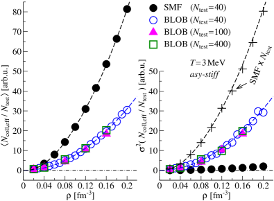
Figure 1: Mean-value (left) and variance (right) of the number of effective in-medium collisions per nucleon and per unit time $\delta t=1$ fm/$c$ for SMF (full black circles) and BLOB, as a function of density. The different open symbols correspond to BLOB calculations with different number of test particles. The dashed-lines on the left panel represent fits to mean-value spectra and they are replotted identically in the right panel, for comparison. The crosses in the righ panel correspond to the SMF variance (black dots) multiplied by $N_{\textrm{test}}$. An asy-stiff parameterisation is used for the symmetry energy (the characteristics of the interactions are defined in Sec. IV).

At variance with the above description, the stochastic term in Eq. (7) can be kept separate and treated as a stochastic force related to an external potential $U^{\prime}$, like in the corresponding semi-classical stochastic mean field (SMF) model Colonna1998 . This leads to treatments where fluctuations are implemented only in the coordinate space, i.e. they are projected on the spacial density. The difference between Eq. (9) and usual stochastic mean-field approaches is that those latter build fluctuations from introducing a well adapted external force or a distribution of initial conditions which should be accurately prepared in advance. On the contrary, Eq. (9) introduces fluctuations in full phase space and let them develop spontaneously and continuously over time in a dynamical process.

Fig. 1 illustrates how this difference affects the statistics of effective in-medium collision (i.e. not Pauli blocked); it compares SMF and BLOB calculations performed in nuclear matter at $3$ MeV temperature and at different densities in stable conditions, i.e. keeping the system uniform, and at equilibrium, i.e. when the average collision rate is constant in time (these conditions are described in details in Sec. IV). As a general trend, larger densities provide a larger number of collision candidates, so that, even if also the difficulty in relocating collision partners increases due to Pauli blocking, the resulting number of effective collisions per nucleon grows significantly with density. Despite the use of the same nucleon-nucleon cross section (which produces equal rates of attempted collisions per nucleon for all the employed approaches, not shown), the number of effective collisions per nucleon differs in the two models due to the different treatment of the Pauli blocking, which is more severe in BLOB, owing to the nucleon wave packet extension (for instance, at $\rho^{0}=0.16$ fm³, large Pauli rejection rates, equal to 98% in BLOB and to 95% in SMF, result in different effective collision rates, see discussion in appendix A). The main difference emerging from the comparison in Fig. 1 is that the variance of the number of effective collisions per nucleon amounts to the mean value reduced by a factor $N_{\textrm{test}}$ in the SMF case, while it equals the mean without any dependence on $N_{\textrm{test}}$ in the BLOB case (several values of $N_{\textrm{test}}$ produce equal results). Such study confirms that, while in SMF fluctuations are strongly reduced in proportion to the quantity $N_{\textrm{test}}$, in BLOB fluctuations have large amplitude and exactly equal the mean value, according to the Poisson statistics Burgio1991 . The quantification of such amplitude is the subject of the following sections.

III Strategy: comparing BL approaches in nuclear matter to the Fermi-liquid behaviour

The purpose of stochastic one-body approaches with collisional correlations like SMF or BLOB is introducing aspects of the Fermi liquid behaviour, including fluctuations Lifshitz1958 ; Pines1966 , in the description of heavy-ion collisions Pethick1988 .

In the following, we check how Eq. (9) handles isoscalar and isovector fluctuations of the one-body density, in equilibrated nuclear matter, with the aim of demonstrating that its implementation is better suited than approximate methods, like SMF, to sample the development of inhomogeneities (equivalent process to fragment formation in finite open systems) and the related observables. We therefore compare results obtained with BLOB and SMF.

III.1 Fluctuations in nuclear matter:
analytic estimate

Let us consider nuclear matter at low temperature. Either from the stochastic fluctuating residual term of the BLOB treatment or from an external stochastic force in the SMF approach, we introduce a small disturbance in uniform matter $\delta f(\mathbf{r},\mathbf{p},t)=f(\mathbf{r},\mathbf{p},t)-f^{0}(\mathbf{p},t)$ which lets fluctuations develop in time around the mean trajectory $f^{0}$.

By considering neutron and proton distribution functions, we can further decompose fluctuations in isoscalar modes $\delta f^{\mathrm{s}}$ and isovector modes $\delta f^{\mathrm{v}}$

$$\delta f^{\mathrm{s}} = (f_{\mathrm{n}}-f_{\mathrm{n}}^{0})+(f_{\mathrm{p}}-f_{\mathrm{p}}^{0})$$ (12)

$$\delta f^{\mathrm{v}} = (f_{\mathrm{n}}-f_{\mathrm{n}}^{0})-(f_{\mathrm{p}}-f_{\mathrm{p}}^{0})\;,$$ (13)

corresponding to phase-space density modes where neutrons and protons oscillate in phase or out of phase, respectively. The temporal evolution of both those modes is obtained by applying the BL equation (7) to the phase-space fluctuations. For symmetric matter, and retaining only first-order terms in $\delta f^{\mathrm{q}}$, one obtains:

$$\frac{\partial\delta f^{\mathrm{q}}}{\partial t}+\frac{\mathbf{p}}{m}\cdot\nabla_{\mathbf{r}}\delta f^{\mathrm{q}}-\frac{\partial f^{0}}{\partial\epsilon}\frac{\partial\delta U^{\mathrm{q}}}{\partial\rho^{\mathrm{q}}}\frac{\mathbf{p}}{m}\cdot\nabla_{\mathbf{r}}\delta\rho^{\mathrm{q}}=\frac{\partial f^{0}}{\partial\epsilon}\frac{\mathbf{p}}{m}\cdot\nabla_{\mathbf{r}}U^{\prime}\;,$$ (14)

where the index $\mathrm{q}$ stands either for isoscalar ($\mathrm{q}=\mathrm{s}$) or isovector ($\mathrm{q}=\mathrm{v}$) modes, $f^{0}=f_{\mathrm{n}}^{0}+f_{\mathrm{p}}^{0}$, $U^{q}$ is the mean-field potential in the $q$ channel and $U^{\prime}$ is an external stochastic force (SMF) or a fluctuating stochastic field (BLOB). We dropped the average collision term $I_{\textrm{UU}}$ because we consider small temperatures.

To build our stochastic descriptions we assumed that, at least locally, fluctuations have a small amplitude around their mean trajectory so that $\delta f^{\mathrm{q}}\!\ll\!f^{\mathrm{q}}$. When the system is described as a periodic box, collective modes are associated to plane waves of wave number $\mathbf{k}$. In this case, by expanding on plane waves expressed in Fourier components, we can study the evolution in time of phase space density fluctuations

$$\delta f^{\mathrm{q}}(\mathbf{r},\mathbf{p},t)=\sum_{k}e^{(i\mathbf{k}\!\cdot\!\mathbf{r})}f_{k}^{\mathrm{q}}(\mathbf{p},t)=\sum_{k}e^{(i\mathbf{k}\!\cdot\!\mathbf{r})}e^{(i\omega_{k}t)}f_{k}^{\mathrm{q}}(\mathbf{p})$$ (15)

and undulations in the density landscape $\delta\rho^{\mathrm{q}}(\mathbf{r},t)=\sum_{k}e^{(i\mathbf{k}\!\cdot\!\mathbf{r})}\rho_{k}^{\mathrm{q}}(t)$. Rewritten in Fourier components, Eq. (14) takes the form

$$i\omega_{k}f_{k}^{\mathrm{q}}+i\mathbf{k}\cdot\frac{\mathbf{p}}{m}f_{k}^{\mathrm{q}}-i\frac{\partial f^{0}}{\partial\epsilon}\frac{\partial U_{k}^{\mathrm{q}}}{\partial\rho^{\mathrm{q}}}\mathbf{k}\cdot\frac{\mathbf{p}}{m}\rho_{k}^{\mathrm{q}}=i\frac{\partial f^{0}}{\partial\epsilon}\mathbf{k}\cdot\frac{\mathbf{p}}{m}\mathcal{F}_{k}^{\mathrm{q}}\;,$$ (16)

where $U_{k}^{\mathrm{q}}$ and $\mathcal{F}_{k}^{\mathrm{q}}$ are Fourier components of the potential $U$ and of the stochastic fluctuating field $U^{\prime}$, respectively.

When the fluctuation modes are of stable nature, the response of the system to the action of the stochastic fluctuating field $\mathcal{F}_{k}^{\mathrm{q}}$ determines the equilibrium variance $(\sigma_{k}^{\mathrm{q}})^{2}$ associated to the fluctuation $\rho_{\mathbf{k}}^{\mathrm{q}}$. The inverse Fourier transform of $(\sigma_{k}^{\mathrm{q}})^{2}$ gives the equilibrium variance of spacial density correlations

$$(\sigma_{\rho^{\mathrm{q}}})^{2}\equiv\langle(\delta\rho^{\mathrm{q}}(\mathbf{r}))^{2}\rangle=(2\pi)^{-3}\sum_{\mathbf{k}}(\sigma_{k}^{\mathrm{q}})^{2}d\mathbf{k}$$ (17)

in a cell of volume $\Delta V$ at temperature $T$. At equilibrium, when the level density $\mathcal{N}\equiv(g/h^{3})\int\partial_{\epsilon}f^{0}\mathrm{d}\mathbf{p}$ for a degeneracy $g$ can be defined, these variances are related to the curvature of the free energy density $F^{\mathrm{q}}(k)$ through the fluctuation–dissipation theorem so that

$$(\sigma_{k}^{\mathrm{q}})^{2}=\frac{T}{F^{\mathrm{q}}(k)}\;;\;\;\;(\sigma_{\rho^{\mathrm{q}}})^{2}=\frac{T}{\Delta V}\Big{\langle}\frac{1}{F^{\mathrm{q}}(k)}\Big{\rangle}_{\mathbf{k}}\;,$$ (18)

where $F^{\mathrm{q}}(k)=\partial_{\rho^{\mathrm{q}}}U_{k}^{\mathrm{q}}+1/\mathcal{N}$, and for an average $\langle\cdot\rangle_{\mathbf{k}}$ extending over all $\mathbf{k}$ modes.

On the other hand, for unstable modes, the diffusion coefficient $\mathcal{D}$, or rather its projection on a given unstable mode $k$, $D_{k}$, determines the following evolution for the intensity of response $(\sigma^{\mathrm{q}}_{k})^{2}$ for the wave number $k$ Colonna1993 ; Colonna1994_a :

$$(\sigma^{\mathrm{q}}_{k})^{2}(t)\approx D_{k}\tau_{k}(e^{2t/\tau_{k}}-1)+(\sigma^{\mathrm{q}}_{k})^{2}(t\!=\!0)e^{2t/\tau_{k}},$$ (19)

where both the initial fluctuation seeds $(\sigma^{\mathrm{q}}_{k})^{2}(t\!=\!0)$ and the fluctuation continuously introduced by the collisional correlations contribute to an exponential amplification of the disturbance, characterised by the growth time $\tau_{k}$.

III.2 Scenarios for isovector and isoscalar fluctuations

In the following, starting from Eq. (16), we concentrate on the propagation of isovector modes, which are always of stable nature, and isoscalar modes, with a special focus on unstable conditions.

Isovector fluctuations, based on Eq. (18) and studied in Sec. IV for nuclear matter at several density values, define how isospin distributes among different phases and portions of the system. On the other hand, isoscalar fluctuations developing in mechanically unstable nuclear matter, which rely on Eq. (19), studied in Sec. V, coincide with the process of separation of those portions of the system into fragments. The latter scenario has been intensively investigated Chomaz2004 foremost because in open dissipative systems, like heavy-ion collisions, it corresponds to a catastrophic process which can lead to the formation of nuclear fragments Tabacaru2003 ; Borderie2008 . The size-distribution of fragments and their formation time are ruled by the dispersion relation for wavelengths related to unstable $k$ modes so that, when unstable modes succeed to get amplified, inhomogeneities develop and eventually lead to mottling patterns at later times. Then, in this case, isovector fluctuations define the isotopic features of fragments and their connection to the symmetry energy Colonna2013 .

IV Results on isovector fluctuations

Isovector effects in nuclear processes may arise from different mechanisms Baran2012 ; DiToro2003 , like the interplay of isospin and density gradients in the reaction dynamics, or nuclear cluster formation, or the decay scheme of a compound nucleus. In systems undergoing a nuclear liquid-gas phase transition, a role is played also by isospin distillation Chomaz2004 ; Baran2005 , a mechanism which consists in producing a less symmetric nucleon fraction in the more volatile phase of the system along the direction of phase separation in a $\rho_{n}$–$\rho_{p}$ space, as an effect of the potential term in the symmetry energy Ducoin2007 ; Colonna2008 .

Along with these analyses, it is particularly instructive to investigate the developing of isovector fluctuations, around the mean trajectory, in two-component nuclear matter.

IV.1 Preparation of a stable and uniform system

We consider nuclear matter with periodic boundary conditions. We refer the reader to the appendix B for details on the parameters chosen for the calculations in the following sections.

Selecting isovector modes ($\mathrm{q}\rightarrow\mathrm{v}$) in Eq. (16), the phase-space density corresponds to $f^{\mathrm{v}}=f_{\mathrm{n}}-f_{\mathrm{p}}$. In order to select the isovector behaviour, we keep only the isovector contribution in the nuclear potential. Indeed, in absence of isoscalar terms, the system is stable at all density values $\rho_{0}$ and one can investigate how isovector fluctuations depend on $\rho_{0}$.

$$U^{\mathrm{q}}\rightarrow U^{\mathrm{v}}=2[(\rho_{n}-\rho_{p})/\rho^{0}]E_{\textrm{sym}}^{\textrm{pot}}\;,$$ (20)

where $\rho^{0}$ is the uniform-matter density and $E_{\textrm{sym}}^{\textrm{pot}}$ is the potential term in the symmetry energy. Following the procedure of ref. Colonna2013 , $U_{k}^{\mathrm{v}}$ is obtained from the above quantity by introducing an interaction range through a Gaussian smearing $g_{\sigma}$ of width $\sigma$, and by taking the Fourier transform; its derivative with respect to $(\rho_{n}\!-\!\rho_{p})$ yields

$$F^{\mathrm{v}}(k)=(2/\rho^{0})E_{\textrm{sym}}^{\textrm{pot}}(\rho^{0})g_{\sigma}(k)+1/\mathcal{N}\;.$$ (21)

Thus, from Eq. (18), we obtain the relation:

$$F_{\textrm{eff}}^{\mathrm{v}}=\frac{T}{2\Delta V}\frac{\rho^{0}}{(\sigma_{\rho^{\mathrm{v}}})^{2}}=\frac{T}{2\Delta V}\frac{\rho^{0}}{\langle[\delta\rho_{n}(\mathbf{r})-\delta\rho_{p}(\mathbf{r})]^{2}\rangle}\;,$$ (22)

where $F_{\textrm{eff}}^{\mathrm{v}}$ can be assimilated to an effective symmetry free energy which, at zero temperature and neglecting surface effects, coincides with the symmetry energy $E_{\textrm{sym}}(\rho^{0})$.

In conventional BUU calculations, however, the smearing effect of the test particles introduces a corresponding scaling factor Colonna1994_a , so that $F_{\textrm{eff}}^{\mathrm{v}}\approx N_{\textrm{test}}E_{\textrm{sym}}$. Such scaling actually reduces drastically the isovector fluctuation variance produced by the UU collision term. In the following, we investigate how the collision term used in the BLOB approach differs from the UU treatment. Since the former is not an average contribution and it acts independently of the number of test particles, we expect a larger isovector fluctuation variance.

To prepare a transport calculation, the system is initialised with a Fermi-Dirac distribution at a temperature $T=3$ MeV; it is then sampled for several values of $\rho^{0}$ and the potential, restricted to the only isovector contribution, is tested for a stiff and a soft density dependence of the symmetry energy for symmetric matter (see appendix B).

IV.2 isovector fluctuation variance and symmetry energy

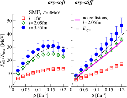
Figure 2: The effective symmetry energy, scaled by $N_{\textrm{test}}$, as extracted from SMF simulations, using Eq. (22), for nuclear matter at temperature $T$ = 3 MeV and at several density values. The different symbols correspond to the three edge sizes $l$ of the cells over which the isovector variance is evaluated. Two parametrizations of the symmetry energy are considered in the calculations: asy-soft (left panel) and asy-stiff (right panel). In both panels, the dot-dashed line represents the analytical expression of the symmetry energy. For the asy-stiff case (right panel), an SMF calculation where the collision term is suppressed is also shown for the edge size $l$ = 2.05 fm (full violet line). Error bars indicate the standard deviation of the $F_{\textrm{eff}}^{\mathrm{v}}/N_{\textrm{test}}$ distribution obtained considering several time instants within a large interval at equilibrium.

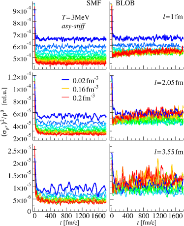
Figure 3: Isovector variance as a function of time calculated, in a single event, with SMF (left) and BLOB (right), for different values of the system density, corresponding to the different colors and ranging from 0.02 fm^-3 (blue line) to 0.2 fm^-3 (red line). Cells of different size $l$ are considered in the calculations: $l$ = 1 fm (top panels), $l$ = 2.05 fm (middle panels) and $l$ = 3.55 fm (bottom panels). An asy-stiff form of the symmetry energy is considered.

From a set of calculations for different densities ranging from $\rho^{0}=0.02$ to $\rho^{0}=0.2$ fm^-3 we obtain a numerical solution of the r.h.s. of Eq. (22) for SMF. We use $N_{\textrm{test}}$ = 40. We consider an equilibrium temperature extracted for each density bin from the slope of the Fermi-Dirac distribution evolved in time. The isovector variance $(\sigma_{\rho^{\mathrm{v}}})^{2}$, calculated in cells of edge size $l=1$, $l=2.05$ and $l=3.55$ fm, is multiplied by $N_{\textrm{test}}$, in order to extract $F_{\textrm{eff}}^{\mathrm{v}}$ and to compare it with the symmetry energy $E_{\textrm{sym}}$. The comparison, shown in Fig. 2, is satisfactory and it is the closest in shape to $E_{\textrm{sym}}$ for larger cells than $l=1$ fm but, however, the large scaling factor $N_{\textrm{test}}$ has to be taken into account. The better agreement in larger cells reflects the decreasing importance of surface effects, so that the calculation gets close to the (volume) symmetry energy.

We notice that an equivalent calculation where the collision term is suppressed yields identical distributions; such collisionless calculation corresponds to switching off the collision term. The need of scaling by $N_{\textrm{test}}$ to recover the expected fluctuation value reflects the fact that isovector fluctuations are not correctly implemented in SMF. Indeed, much attention is paid in the model to a good reproduction of isoscalar fluctuations and amplification of mean-field unstable modes, by introducing an appropriate external field Colonna1998 . On the other hand, explicit fluctuation terms are not injected in the isovector channel in SMF. In this case, one just obtains the fluctuations related to the use of a finite number of test particles which, as far as the Fermi statistics is preserved, amount to the physical ones divided by $N_{\textrm{test}}$. These results completes the study of ref.Colonna2013 concerning SMF.

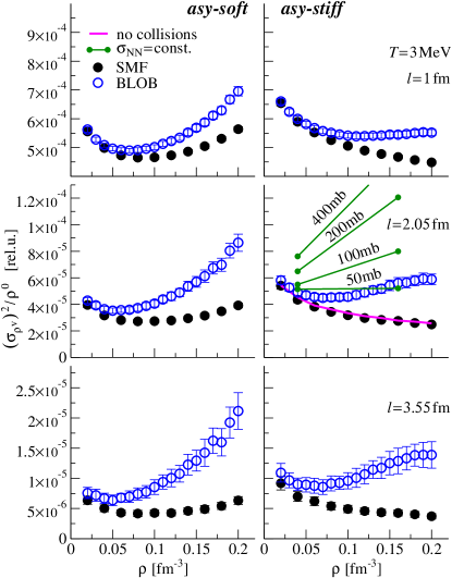
Figure 4: The isovector variance, at equilibrium, as a function of the system density, calculated with SMF (full circles) and BLOB (open circles), for two parametrizations of the symmetry energy: asy-soft (left panels) and asy-stiff (right panels) Cells of different size $l$ are considered in the calculations: $l$ = 1 fm (top panels), $l$ = 2.05 fm (middle panels) and $l$ = 3.55 fm (bottom panels). For one case (asystiff, $l=2.05$ fm) other calculations are shown: SMF with the collision term suppressed (full violet line), and BLOB calculations for different constant values of $\sigma_{\textrm{NN}}$ (green lines). Error bars indicate the standard deviation of the isovector variance distribution obtained considering several time instants within a large interval at equilibrium.

We now turn to BLOB calculations. Fig. 3 shows that the isovector variance in BLOB results larger than in SMF. Such difference is therefore the effect of the treatment of collisional correlations in BLOB, which displays a dependence with the system density. In particular, the low-density limit of the spectrum corresponds to a situation where the collision rate is vanishing. In this case, the BLOB procedure is practically ineffective (see also the discussion in Section V.A) and all approaches converge to the same isovector variance, just related to the finite number of test particles employed. At larger density than saturation ($\rho\geq 0.18$ fm^-3), BLOB displays a longer path to convergence which is due to the difficulty of relocating large portions of phase space in binary collisions without violating Pauli blocking.

Fig. 4 condenses and extends the information of Fig. 3 by displaying the density evolution of the isovector variance attained at equilibrium as evaluated in cells of different size $l$, for asy-stiff and asy-soft forms of the symmetry energy. The SMF data correspond to those analysed in Fig. 2. The BLOB spectra progressively deviate from SMF data for increasing density. Such deviation increases for larger cell sizes indicating that the isovector fluctuations are better built in large volumes Rizzo2008 . This is related to the variety of configurations, concerning shape and extension of the nucleon wave packet, which occur in the implementation of the fluctuating collision integral. This introduces a smearing of fluctuations on a scale comparable to the wave-packet extension in phase space. However, the gain in isovector variance exhibited by the BLOB approach, indicates that the dependence on $N_{\textrm{test}}$ is partially reduced with respect to the SMF scheme.

IV.3 Interference between mean-field propagation, collisional and numerical correlations

According to Eq. (9), the BLOB approach should introduce and revive fluctuations continuously. The agglomeration procedure employed in BLOB is actually able to construct agglomerates of test particles of the same isospin species and which are located around local density maxima in random selected phase-space cells: this technique should preserve at least partially the isovector correlations in the system, contrarily to the usual BUU technique which smears them out. This advance with respect to BUU is however not sufficient because of the concurrent effects associated with the mean-field dissipation. Indeed, fluctuations are propagated according to a total inverse relaxation time

$$1/\tau_{k}^{\prime}=1/\tau_{k}^{\textrm{coll}}+1/\tau_{k}^{\textrm{m.f.}}\;,$$ (23)

so that, if the collisional rate is too small, they are damped by the mean-field dynamics before they can reach a sizeable amplitude.

Moreover, even in absence of any explicit fluctuation seed, the dynamics is actually affected by a numerical noise, due to the use of a finite number of test particles in the numerical resolution of the transport equations; such spurious contribution imposes the dependence of $(\sigma_{\rho^{\mathrm{q}}})^{2}$ on $N_{\textrm{test}}$ Colonna1993 . If this latter effect may be negligible with respect to the large isoscalar fluctuations developing in presence of mean-field instabilities (see next Section), it becomes a highly interfering contribution for the isovector modes. In other words, the numerical noise leads to an effective diffusion coefficient $D_{k}^{\prime}=D_{k}+D_{k}^{\textrm{noise}}$. If a small number of test particles is considered, and two-body collisions are not so frequent, then $D_{k}^{\textrm{noise}}$ prevails over $D_{k}$, causing a deviation of the fluctuation amplitude from the correct value.

For these reasons, though in principle the fluctuation equilibrium value, as deduced from BLOB, should not depend on the details of the nucleon-nucleon cross section $\sigma_{\textrm{NN}}$ and on the number of test particle employed, our results depend significantly on both ingredients.

Two ways can be tested to get a deeper insight into this problem: either the collision term should be considerably enhanced, or fluctuations generated by test particles should be prevented.

The first solution can be achieved by simply multiplying $\sigma_{\textrm{NN}}$ by a large factor, with the drawback of then handling incorrect collision rates. Of course, this is not a problem if one is interested in equilibrated matter, as in the present case, but it would be crucial when dealing with non-equilibrium processes, such as nuclear reactions. Some tests in the first direction are proposed in Fig. 4, by employing a constant $\sigma_{\textrm{NN}}$ with progressively larger values, showing that the isovector variance grows with the collision rate, as we expect on the basis of the arguments discussed above.

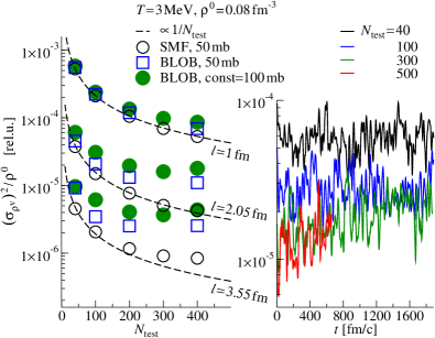
Figure 5: Left: The isovector variance, at equilibrium, as a function of the number of test particles, $N_{\textrm{test}}$, as obtained in SMF simulations (open circles) and in BLOB calculations (open squares), using a constant $\sigma_{\textrm{NN}}$=50mb, for nuclear matter at density $\rho^{0}$ = 0.08 fm^-3 and temperature $T=3$ MeV. BLOB calculations are also shown for $\sigma_{\textrm{NN}}$=100mb (green full circles). Cells of different size $l$ are considered, as indicated on the figure. Dashed lines represent a fit of SMF simulations, assuming a trend proportional to the inverse of the test particle number. Right: Time evolution of the isovector variance, as obtained in a single event, for BLOB calculations with constant $\sigma_{\textrm{NN}}$=100mb and $l=2.05$fm. The different curves correspond to different number of test particles employed in the simulations. The asy-stiff form of the symmetry energy is considered.

The second check would consist in employing the largest possible number of test particles per nucleon. In this case, the collisionless transport model would ideally correspond to the Vlasov approach and, when collisional correlations are introduced, interferences with spurious stochastic sources can be highly reduced. However, interference effects with the mean-field propagation can still be important, depending on the collision rate. As far as numerical complexity can be handled, Fig. 5, left, illustrates such situation: SMF calculations show a behaviour $\propto 1/N_{\textrm{test}}$, independently of $\sigma_{\textrm{NN}}$. On the other hand, in the BLOB case one observes that, especially in the largest cells, where fluctuations are more effective, the corresponding variance deviates more and more, for large test particle numbers, from the SMF results, reaching a kind of saturation value. The latter depends on the cell size, $l$, and on the cross section employed (see also the discussion above). Fig. 5, right, shows the time evolution of the fluctuation variance. It appears that for a small number of test particles (up to 100) the variance oscillates around its initial value, which is essentially associated with the numerical noise and scales as $1/N_{\textrm{test}}$. Increasing the number of test particles, the numerical noise gets smaller and the BLOB fluctuation source prevails on it, building up a fluctuation variance which is larger than the initial value. However, since we are considering systems at low temperature, the number of nucleon-nucleon collisions is extremely low and insufficient to rapidly introduce a pattern of isovector correlations, unless one employes very high values for the cross section: the isovector variance shows in fact a very gentle growth.

In conclusion, the BLOB fluctuation source term works well in conditions where the collision rate is large enough, as compared to the mean-field propagation and to the spurious dissipative terms associated with the finite number of test particles. These conditions are likely reached in the first, non equilibrated stages of heavy ion collisions, but not necessarily for equilibrated nuclear matter at low temperature. In the latter case, the variance associated with the fluctuating collision integral can be recovered by artificially increasing the employed $\sigma_{\textrm{NN}}$. Indeed, as shown in Fig. 4 and Fig. 5, we observe that the fluctuation variance built by BLOB may deviate significantly from the SMF results, being up to a factor ten larger, especially when considering fluctuations in larger cells ($l\approx$ 2 to 3 fm).

V Results on isoscalar fluctuations

If fluctuation seeds are introduced in homogeneous neutral nuclear matter at low temperature, Landau zero-sound Landau1957 collective modes should stand out and propagate in the system. In the present section we analyse whether the BLOB approach is able to develop, as aimed, isoscalar fluctuations of correct amplitude in nuclear matter spontaneously, and not from an external contribution, when the system is placed in a dynamically unstable region of the equation of state Belkacem1994 , like the spinodal zone. In this circumstance, as soon as fluctuation seeds are generated, unstable zero-sound waves should be amplified in time. In the opposite situation, in conditions of mechanical stability, undamped stable zero-sound waves propagate. Then, for stable configurations, the same argumentations of Sec. IV hold and, in this case, the fluctuation variance is linked to matter incompressibility.

V.1 Sampling zero-sound propagation in mechanically stable and unstable nuclear matter

The propagation of fluctuations in nuclear matter can be described in a linear-response approximation Colonna1994_a as far as deviations from the average dynamical path are small. In Eq. (16), by selecting isoscalar modes ($\mathrm{q}\rightarrow\mathrm{s}$, we drop the $\mathrm{s}$ index in the following), and setting residual contributions to zero, we obtain a linearised Vlasov equation in terms of frequencies $\omega_{k}$ to describe stable matter with isoscalar contributions:

$$\omega_{k}f_{k}+\mathbf{k}\cdot\frac{\mathbf{p}}{m}f_{k}-\frac{\partial f^{0}}{\partial\epsilon}\frac{\partial U_{k}}{\partial\rho}\mathbf{k}\cdot\frac{\mathbf{p}}{m}\rho_{k}=0\;.$$ (24)

Different wave numbers $\mathbf{k}$ are decoupled, each linked to a collective solution $f_{k}$ given by the Fourier-transformed equation of motion. By applying the self-consistency condition $\rho_{k}=(g/h^{3})\int f_{k}(\mathbf{p})\mathrm{d}\mathbf{p}$, we obtain the dispersion relation for the propagation of density waves in Fermi liquids at $T=0$ :

$$1=\frac{g}{h^{3}}\frac{\partial U_{k}}{\partial\rho}\int\frac{\partial f^{0}}{\partial\epsilon}\frac{\mathbf{k}\cdot\mathbf{p}/m}{\omega_{k}+\mathbf{k}\cdot\mathbf{p}/m}\mathrm{d}\mathbf{p}\;.$$ (25)

where $\omega_{k}$ and $-\omega_{k}$ are pair solutions due to the invariance $\mathbf{p}\leftrightarrow-\mathbf{p}$. As well documented in the literature, at $T=0$ eigenmodes $f_{k}$ depend only on states near the Fermi level. Indeed, the momentum integral is restricted to the Fermi surface because $\partial_{\epsilon}f^{0}\approx-\delta(\epsilon-\epsilon_{\textrm{F}})$, being $\epsilon_{\textrm{F}}$ the Fermi energy. The dispersion relation reduces to an expression where solutions correspond to sound velocities $s=\omega_{k}/(kv_{\textrm{F}})$ in units of Fermi velocity $v_{\textrm{F}}=p_{\textrm{F}}/m$. In this case, introducing the Landau parameter

$$F_{0}(\mathbf{k})=\mathcal{N}_{0}\partial_{\rho}U_{k}=(3/2)(\rho^{0}/\epsilon_{\textrm{F}})\partial_{\rho}U_{k}\;,$$ (26)

where $\mathcal{N}_{0}=\mathcal{N}(T=0)$ is linked to the number of levels at Fermi energy $\epsilon_{\textrm{F}}$, the dispersion relation takes the form Kalatnikov1958 :

$$1+\frac{1}{F_{0}}=L(s)=\frac{s}{2}\textrm{ln}\left(\frac{s+1}{s-1}\right)\;,$$ (27)

where the Lindhard function, $L(s)$ has been introduced. In correspondence to the effective interaction employed, reflected in the potential shown in Fig. 6a, the Landau parameter is illustrated in Fig. 6b, while Fig. 6c presents the roots of the dispersion relation, corresponding to the effective interaction.

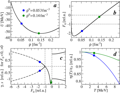
Figure 6: (a) The isoscalar mean-field potential as a function of the density. The dots indicate the two density values considered in SMF/BLOB simulations. (b) The Landau parameter $F_{0}$ as a function of the density. (c) real (for $F_{0}>0$) and imaginary (for $F_{0}<0$) roots of the dispersion relation; the spinodal region corresponds to $F_{0}<-1$, the region for $-1<F_{0}<0$ corresponds to Landau damping and positive values of $F_{0}$ define stable modes. Blue dots indicate the $\gamma$ values corresponding to the density $\rho^{0}$ = 0.053 fm^-3. The $\gamma$ value corresponding to $\rho^{0}$ = 0.14 fm^-3 is beyond the interval shown in the figure (in the direction of the green arrow). (d) The chemical potential, divided by the Fermi energy, as a function of the temperature $T$, for the two density values considered in the calculations: $\rho^{0}$ = 0.053 fm^-3 (blue line) and $\rho^{0}$ = 0.14 fm^-3 (green line). The dots correspond to the temperature value ($T=3$ MeV) considered in the simulations.

V.2 Warm systems and interaction range

Eq. (27) is only valid at zero temperature. When the temperature is significant, two-body collision rates become prominent and these mean-field dominated zero-sound waves are absorbed and taken over by hydrodynamical first-sound collective modes. Since our approach exploits two-body collisions to introduce fluctuations in a self-consistent mean field, we expect the possible occurrence of a zero-to-first-sound transition which, at variance with other Fermi liquids Abel1966 , should be even smeared out due to the small values taken by the Landau parameter $F_{0}$ in nuclear matter. It was found that, depending on how the system is prepared and on the type of collective motion, such transition should arise in a range of temperature from 4 to 5 MeV and occur as late as 200 fm/$c$ Larionov2000 ; Kolomietz1996 . In practice, zero-sound modes associated to wave vectors $\mathbf{k}$ characterise the system as long as the corresponding phase velocity exceeds the velocity of a particle on the Fermi surface $v_{\textrm{F}}$ or, equivalently, as long as the corresponding frequency $\omega_{k}$ is much higher then the two-body collision frequency $\nu$. These premises imply that, after defining a homogeneous initial configuration at a suited finite and not so large temperature, we should study early intervals of time to extract properties of the response function which can be compared with zero-sound conditions.

Temperature effects can be included, in an approximate manner, considering the low temperature Sommerfeld expansion of the chemical potential $\mu$(T):

$$\frac{\mu(T)}{\epsilon_{\textrm{F}}}\approx 1-\frac{\pi^{2}}{12}\left(\frac{T}{\epsilon_{\textrm{F}}}\right)^{2}\;,$$ (28)

which is illustrated in Fig. 6d.

As a further modification, we consider that zero-sound conditions also present a strong dependence on the interaction range. This latter can be included in the dispersion relation by applying a Gaussian smearing factor of the mean-field potential which is related to the nuclear interaction range in configuration space Colonna1994 ; Kolomirtz1999 .

$$U\rightarrow U\otimes g(k),\;\;\textrm{with}\;\;g(k)=\textrm{e}^{-\frac{1}{2}(k\sigma)^{2}}\;,$$ (29)

From Eq. (28) and Eq. (29), the dispersion relation, Eq. (27), involves an effective Landau parameter Colonna1994 ,

$$\widetilde{F}_{0}(k,T)=\frac{\mu(T)}{\epsilon_{\textrm{F}}}{F}_{0}g(k)\;.$$ (30)

Mechanically unstable conditions are experienced when the evolution of local density $\rho$ and pressure $P$ implies that the incompressibility is negative. This situation is reflected by an effective Landau parameter $\widetilde{F}_{0}(k=0,T)$ smaller than $-1$, so that

$$\frac{\partial P}{\partial\rho}\approx\frac{2}{3}\epsilon_{\textrm{F}}[1+\widetilde{F}_{0}(k=0,T)]\;\;<\,0\;,$$ (31)

and it corresponds to imaginary solutions of the dispersion relation Pomeranchuk1959 . By replacing $s\rightarrow i\gamma$, the relation yielding imaginary solutions can be put in the form:

$$1+\frac{1}{\widetilde{F}_{0}(k,T)}=\gamma\,\textrm{arctan}\frac{1}{\gamma}\;.$$ (32)

The growth rate $\Gamma_{k}=1/\tau_{k}$ is obtained from the solutions of the dispersion relation

$$|\gamma|=\frac{|\omega_{k}|}{kv_{\textrm{F}}}=\frac{1}{\tau_{k}kv_{\textrm{F}}}\;,$$ (33)

As far as the Fermi statistics is kept in a sufficiently large periodic portion of mechanically unstable nuclear matter, and a fluctuation source term is acting, the expectation is that the intensity of the response should be amplified with the growth rate $\Gamma_{k}$ imposed by the mean-field potential $U$ as a function of the unstable mode $\mathbf{k}$.

V.3 Obtaining the dispersion relation

To check such expectation numerically through a BL transport approach we keep the same scheme for the definition of the box metrics as in Sec. IV; the isoscalar density variance is calculated over cells of edge size $l=1$ fm. We now use the full parametrisation of the energy potential per nucleon Eq. (38), where we use a stiff density dependence of the symmetry energy (the same parametrisation was analysed in ref. Colonna1997 ). Nuclear matter is isospin symmetric and it is initially uniform and prepared at a temperature $T=3$ MeV and at densities equal to $\rho^{0}\!=\!0.053$ and $0.14$ fm^-3. Fig. 6 illustrates the values taken by the potential and by the dispersion relation related to these choices. The collision term involves the usual isospin- and energy-dependent free nucleon-nucleon cross section with an upper cutoff at $\sigma_{\textrm{NN}}=50$ mb.

Within the dynamical calculation we should register at each interval of time $t$ the density in all cells of edge size $l$ of the lattice which constitutes the periodic system of edge size $L$. A specific cell can be identified by the vector $\mathbf{n}^{\prime}$. Having introduced such a lattice, the perturbation wave number $k$ can be expressed as $k=2\pi n/L$, where $n$ is the modulus of a vector ranging from 1 to $n_{\textrm{max}}=L/l$ along each of the three spacial directions. Then the amplitude of the isoscalar fluctuation of a mode $k$ is obtained from the Fourier transform, $F_{\mathbf{k}}$, of the space density

$$\sigma^{2}_{k}(t)=\langle F_{\mathbf{k}}^{2}(t)\rangle=\frac{1}{l^{3}}\Big{\langle}\Big{[}\sum_{\mathbf{n}^{\prime}}\rho_{\mathbf{n}^{\prime}}(t)\,\mathrm{exp}\big{(}ia\mathbf{n}\!\cdot\!\mathbf{n}^{\prime}\big{)}\Big{]}^{2}\Big{\rangle}$$ (34)

$$\propto\Big{\langle}\Big{[}\sum_{\mathbf{n}^{\prime}}\rho_{\mathbf{n}^{\prime}}(t)\textrm{cos}(a\mathbf{n}\!\cdot\!\mathbf{n}^{\prime})\Big{]}^{2}\!+\!\Big{[}\sum_{\mathbf{n}^{\prime}}\rho_{\mathbf{n}^{\prime}}(t)\textrm{sin}(a\mathbf{n}\!\cdot\!\mathbf{n}^{\prime})\Big{]}^{2}\Big{\rangle}\;,$$

where $a=2\pi l/L$ and the average is extended over all orientations of $\mathbf{k}$.

The distribution of ratios $\tilde{\sigma}^{2}_{k}(t)=\sigma^{2}_{k}(t)/\sigma^{2}_{k}(t=0)$, averaged over several dynamical paths, is shown at different time intervals in Fig. 7 for the two density choices. It should be noticed that the initial fluctuation amplitude is due to the finite number of test particles employed in the calculations. However, as soon as the BLOB term starts to act, fluctuations of larger amplitude are built up (see also the discussion in Section V.A), and further amplified by the unstable mean-field. The system prepared at $\rho^{0}\!=\!0.053$ fm^-3, inside the spinodal region, exhibits a clear growth of instabilities as a function of time for some $k$ waves, while the system prepared at $\rho^{0}\!=\!0.14$ fm^-3, outside the spinodal region, presents an evolution of the response intensity corresponding to a more gentle growth in a Landau-damping regime. However, even in this latter case, fluctuations reach a significant amplitude, owing to the small compressibility value in the density region considered, but cluster formation is not observed.

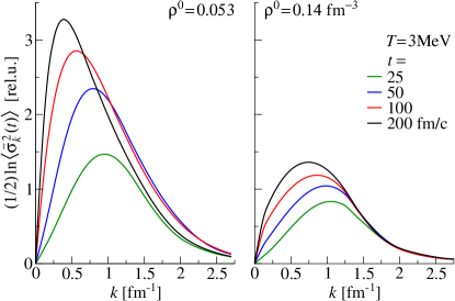
Figure 7: BLOB calculation. Response intensity $\tilde{\sigma}^{2}_{k}(t)=\sigma^{2}_{k}(t)/\sigma^{2}_{k}(t=0)$, averaged over 100 dynamical paths, as a function of the wave number $k$. The different curves correspond to different time instants, as indicated on the figure. Left panel: results for $\rho^{0}\!=\!0.053$ fm^-3 (spinodal). Right panel: results for $\rho^{0}\!=\!0.14$ fm^-3 (Landau damping).

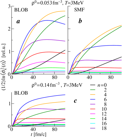
Figure 8: Early time evolution of the response intensity $\tilde{\sigma}^{2}_{k}(t)$ for several modes ($n=j$ stands for all $k$ modes within $2\pi(j-1)/L\leq k<2\pi j/L$). (a) BLOB calculations for $\rho^{0}\!=\!0.053$ fm^-3 (spinodal). (b) SMF calculations for $\rho^{0}\!=\!0.053$ fm^-3. (c) BLOB calculations for $\rho^{0}\!=\!0.14$ fm^-3 (Landau damping).

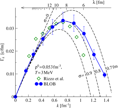
Figure 9: BLOB calculations for nuclear matter at $\rho_{0}$ = 0.053 fm^-3 and temperature $T$ = 3 MeV: The growth rate $\Gamma_{k}$ , as extracted from the simulations (see Eq.(35)), is plotted as a function of the wave number $k$ (full line with dots). Uncertainties are evaluated from the linear-response fit. The dashed lines correspond to analytical predictions, obtained solving Eq.(32) with different values of the width $\sigma$ of the Gaussian smearing factor. For comparison, a calculation in one-dimension within the approach of ref. Rizzo2008 is also shown (green diamonds).

Correspondingly, the early evolution in time of $\tilde{\sigma}^{2}_{k}(t)$ is analysed in Fig. 8 for the two density choices. For the leading modes, one can consider a linear fit of the quantity plotted in Fig. 8a, in intervals ranging from around 20fm/$c$ to time instants close to saturation (see Eq. 19). The very initial path is excluded from the fit because, as previously mentioned, the fluctuation mechanism sets in spontaneously after that a sufficient number of collisions has occurred, and does not emerge from suited initial conditions. Differences from the ideal linear response in the growing side of single modes indicate a more complex behaviour, resulting from the coupling of different wavelengths and the tendency toward a chaotic evolution Baldo1995 ; A SMF calculation is also presented for the unstable system, where the linear growth of the leading modes is initially comparable to the BLOB approach and deviates at later times. This behaviour is due to the efficiency of the collision term in the BLOB model in reviving fluctuations of correct amplitude, compared to SMF, where fluctuations are not introduced by the collision term. As a consequence, in SMF fluctuations decay by the combination of small wavelengths into larger ones, while in BLOB higher fluctuation amplitudes can be attained before reaching the saturation regime.

The numerical extraction of the growth rate $\Gamma_{k}$, i.e., of the quantity given by the analytic relation of Eq. (33) is obtained from the time derivative (at early time instants) of the amplitude of the isoscalar fluctuation for a given mode $k$ as

$$\Gamma_{k}=\frac{1}{2}\frac{\partial}{\partial t}{\textrm{l}n}\prec\tilde{\sigma}^{2}_{k}(t)\succ\;,$$ (35)

where the average $\prec\cdot\succ$ is taken over several stochastic dynamical trajectories. Such analysis is presented in Fig. 9, where the numerical calculation, averaged over 100 events, is compared to the analytic result of Eq. (33). The range of the interaction, as an effect of the implemented surface term, would correspond to a Gaussian smearing of around $\sigma=0.8$ fm to $\sigma=0.9$ fm. We infer that BLOB reproduces consistently the expected dispersion relation within the uncertainties of the linear regression. Another calculation, also based on the same mean-field, but which employs the earlier approach of ref. Rizzo2008 , also solved in three dimensions but with fluctuations developing along one axis of configuration space, produces a similar result. While BLOB keeps the different unstable modes decoupled for a more extended interval of time during their early growth, also resulting into a larger ultraviolet cutoff, the other approach (green points) presents some alterations due to the combining of unstable modes, where small-wavelength ($n\!>\!7$) are gradually absorbed by large-wavelength ($n\!=\!0,n\!=\!1$). The effect in this case is an increase of the growth rate for small $k$ values and it signs the entrance of the chaotic behaviour which characterises larger times Jacquot1996 . The largest $k$ modes, corresponding to wavelengths which drop below the Gaussian smearing width $\sigma$ are meaningless. As a final result of this study, the leading modes are found in a wavelength range from 8 to 9fm, and for a growth time $\tau_{k}$ of around 30fm$/$c.

VI Connecting nuclear matter to open systems

The aim of this work is studying the effect of isovector and isoscalar fluctuations. The ultimate purpose of the transport approaches discussed therein is describing the formation of nuclear fragments in a fermionic system and their properties through the combination of these two types of fluctuating modes, as will be detailed more diffusely in forthcoming works. In particular, isovector fluctuations, on top of other isospin transport effects, impose that the isospin content is distributed through a density-dependent process of distillation, supplemented by an isotopic variance. The onset of isoscalar modes is then responsible for breaking the uniformity of the density landscape and eventually partitioning it into nuclear fragments, where the isospin properties of the initial nesting sites are preserved. The isoscalar and isovector mechanisms should therefore be intimately connected in order to describe fragment formation.

VI.1 Fragment formation: patterns and time scales

Qualitatively, we may underline some connection between the wavelengths involved in the dispersion relation analysed in Fig. 9, and fragment formation Matera2000 , considering that at the system density $\rho^{0}$ the leading modes correspond to fragments of mass $A\approx\rho^{0}\lambda^{3}$; for the leading wavelengths, this corresponds to a distribution of sizes peaked around Neon. These results are also in agreement with other previous studies where quantum effects were taken into considerations explicitly Ayik1995 ; Jacquot1997 ; Colonna1998bis ; Norenberg2000 ; Ayik2008 despite a more schematic treatment of fluctuations, or of the whole dynamics (2-dimension treatments, fluctuations propagated from an initial state, spherical geometries). In this respect, BLOB extends these previous attempts to a model that can be applied at the same time to nuclear matter and, rather successfully, to heavy-ion collisions in three dimensions and without any preliminary initialisation of fluctuation seeds Napolitani2013 ; Napolitani2015 .

From the growth time of the leading modes in Fig. 9, we infer that the corresponding process of fragment formation would be rather short, progressing from when the system has been largely diluted. This suggests that the scenario studied in nuclear matter can be quite directly translated to the phenomenology of open systems Chomaz2004 . As an example, Fig. 10 illustrates the correspondence between a portion of nuclear matter (simulated for $T=3$ MeV and $\rho^{0}\!=\!0.053$ fm^-3 for an interaction defined as in Eq. (38) and a hot system formed in the collision ¹³⁶Xe$+^{124}$Sn at 32 $A$MeV for a central impact parameter $b=0$ (such system was studied in an experimental campaign Moisan2012 ; Ademard2014 ). In particular, we observe some analogy between the early time when inhomogeneities emerge in nuclear matter (20fm/$c$) and when fragments start forming in an open system (around 100fm/$c$) right after accessing low-density spinodal conditions (around 80fm/$c$). In both systems, a spinodal signal stands out by exhibiting equal-size inhomogeneities in configuration space within a similar time scale Napolitani2013 , and it is smeared out by fragment recombination later on. At even later times, the evolution is different, in the box calculation clusters continue interacting with each other while in the open system they split apart.

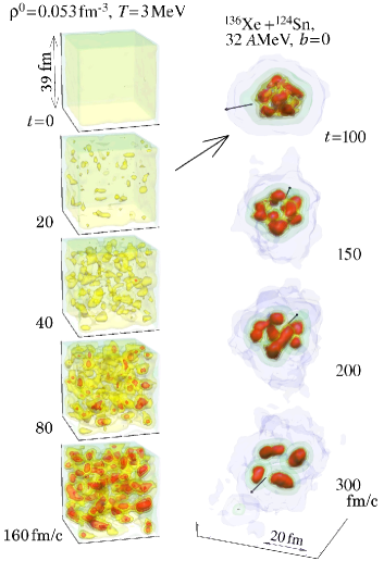
Figure 10: Density-landscape at several time instants for nuclear matter in a periodic box at $\rho^{0}\!=\!0.053$ fm^-3 and T = 3 MeV (left) and in a hot open nuclear system formed in a head-on ¹³⁶Xe+¹²⁴Sn collision at 32 $A$MeV (right); arrows indicate the beam direction. Both simulations employ the BLOB approach with the same mean-field properties. The big arrow proposes an analogy between nuclear matter and the open system in correspondence with the arising of the spinodal instability.

Experimental investigations of heavy-ion collisions at Fermi energies already pointed out that the range of masses given by the dispersion relation of Fig. 9 is actually favoured in multifragmentation mechanisms; the kinematics of the process was also found to be rather explosive. The spinodal mechanism was therefore proposed as a suited description Borderie2001 ; Desesquelles2002 ; BLOB has already been adapted successfully to nuclear collisions and tested over various systems which experience spinodal instability Napolitani2013 ; Napolitani2015 ; Colonna2016 .

VI.2 Isospin content in fragments

Fig. 11 completes the survey, investigating the isospin content in potential ripples containing $N^{\prime}$ neutrons and $Z^{\prime}$ protons for the system ¹³⁶Xe$+^{124}$Sn at 32 $A$MeV. Distributions of isotopic variances are calculated for the most probable mass range around a forming Carbon and a forming Neon (two upper rows). The distributions are studied in an early time span (before that fragments are clearly formed, around 130fm/$c$) and in a late time interval (during fragment formation around 200fm/$c$). They are compared with the analytic distributions obtained at a temperature $T=5.5$ MeV, as extracted from the calculation, and at the local density $\rho$. The isotopic variance (see Eq. (18)) can be studied as the probability of variation $\delta$ around the mean value of $N^{\prime}-Z^{\prime}$ and for a given $A^{\prime}$ yielding the distribution

$$Y\approx\textrm{exp}[-(\delta^{2}/A^{\prime})\,C_{\textrm{sym}}(\rho)/T]\;.$$ (36)

The local density is evaluated either in the (denser) centroid of the potential ripples $\rho_{\textrm{centroid}}$, or averaged all over the volume of the emerging fragments $\widetilde{\rho}$, or, more significantly, corresponding to the matter contained in the volume of the potential ripples $\rho_{\textrm{well}}$. We deduce that, as expected from the calculation in stable nuclear matter discussed above, the isotopic width results underestimated with respect to the analytic prediction of Eq. (18). The difference is still acceptable due to the following two effects. First of all, fluctuations are built out of equilibrium: this implies that the collision rate is higher, generally leading to larger variances. Secondly, in open systems, particle evaporation may contribute in widening the isotopic spectra.

The bottom row of Fig. 11 investigates the average isospin content measured in potential ripples in the corresponding early and late time intervals as a function of the $\rho_{\textrm{well}}$. The mass $A^{\prime}$ grows with the density and the corresponding isospin content decreases, signing a process of isospin distillation.

VI.3 Extent of different clusterisation processes in heavy-ion collisions

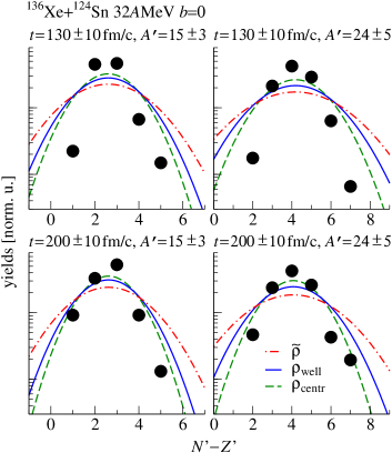
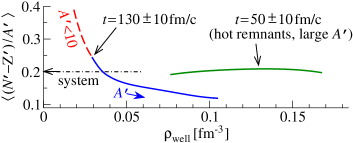
Figure 11: BLOB simulation of head-on ¹³⁶Xe+¹²⁴Sn collisions at 32 $A$MeV. Upper row: Isotopic distribution (full dots) in potential ripples containing $N^{\prime}$ neutrons and $Z^{\prime}$ protons for forming-cluster configurations with masses around $A^{\prime}=15$ (left) and $A^{\prime}=24$ (right) at t = 130 fm/c. The lines correspond to analytic distributions (see Eq.(36)), corresponding to the density extracted from different portions of potential ripples (see text). Middle row: The same as in the upper row, but at t = 200 fm/c. Bottom. Average isospin content measured in potential ripples at two different times, as indicated on the figure, as a function of $\rho_{\textrm{well}}$. Larger density values correspond to pre-fragments of larger mass. The dot-dashed line with an arrow indicates the asymmetry of the projectile-target composite system.

The processes discussed in this work, related to phase-space fluctuations and mechanical instabilities, involve a rich phenomenology of phase transitions and thresholds between very different reaction mechanisms. They may therefore also present some similarities in their outcome with other rather different processes and, in some situations, combine with them. For instance, the onset of instabilities of Rayleigh type is a common process in macroscopic hydrodynamic systems, like classical fluids with a non-negligible surface tension Ashgriz1990 , which has also been proposed as a possible additional scenario for nuclear multifragmentation in heavy-ion collisions Moretto1992 ; Lukasik1997 , in some specific situations. Such process occurs in systems where a dilute core expands into a denser shell (Rayleigh-Taylor instability), or it acts on very deformed systems involving cohesional forces which respond to external perturbations (Plateau-Rayleigh instability). The system in such hydrodynamic scenario develops hole nucleation, evolving into a sponge-like or a filamented configurations which then relax into compact droplets. The mechanism is faster than ordinary fission and density variations of bound matter along the process do not need to be significant.

On the other hand, the spinodal process described above can only occur if the system traverses a specific region of the equation of state, characterised by negative incompressibility where nucleation progresses from a dilute phase, letting blobs of larger density gradually emerge. From a microscopic point of view, it is rather associated to the nuclear liquid-gas phase transition and it requires a time comparable to the equilibration time of the system in reactions at Fermi energies. We point out that, in simulations of heavy-ion collision, the BLOB approach is actually able to describe the interplay between spinodal processes and the above mentioned hydrodynamic effects Napolitani2016 .

Heavy-ion collisions and nuclear matter also involve processes of nuclear cluster formation, from light charge particles to heavier nuclear molecules, but those products emerge from an even different mechanisms Typel2014 , which would require the explicit inclusion of additional correlations in the hierarchy of Eq. (1). Light charged particles related to nuclear clustering have too small size, exceeding the ultraviolet cutoff of the dispersion relation, so that they can not belong to the unstable multipole modes which characterise spinodal fragmentation. Solutions for an explicit treatment of cluster formation are proposed in refs. Danielewicz1991 ; Kuhrts2001 ; Ono2016 . Connections between nuclear clustering and (spinodal) multifragmentation might be proposed, considering that multifragmentation might act on defining nuclear sources with rather complex shape from which clustered structures might eventually emerge.

VII Conclusions

This work presents crucial steps to validate BL transport models applied to a fermionic system, both in stable and mechanically unstable conditions, as far as the development of isoscalar and isovector fluctuations at various densities is concerned. In particular, the amplitude of fluctuations is investigated in relation with the corresponding properties of the nuclear effective interaction. A transport approach constructed by requiring to satisfy the dispersion relation of mean-field unstable modes proves to be suited for the description of nuclear multifragmentation.

In practice, even though technically demanding, the BLOB approach constitutes a conceptually straightforward solution of the BLE in three dimensions. Through a simple renormalisation of the collision term, the Fermi statistics is in fact preserved for a long time and a correct isoscalar fluctuation amplitude is obtained independently of the ingredients of the numerical implementation (like the number of test particles), just associated with the collision rate and the growth time of the unstable modes. Also the fluctuation variance of isovector observables are better treated than in conventional semiclassical approaches, even though the expected variance is still not achieved. Indeed, in the implementation of the fluctuating collision integral, different configurations, varying in shape and extension, are possible to represent the nucleon wave packet. This induces smearing effects on the fluctuation amplitude. Moreover, if the collision rate is very low, the characteristic time scales associated with the construction of collisional two-body correlations are larger than the typical mean-field time scale and the fluctuations are damped by the propagation in the stable mean-field. This explains why, even for equilibrated nuclear matter, the model yields a dependence of the isovector fluctuation amplitude on the nucleon-nucleon cross section. It is also observed that, if two-body collisions are too rare, the numerical noise dominates the dynamics and one obtains a fluctuation variance reduced by a factor $1/N_{\textrm{test}}$ with respect to the expected value, as obtained in standard transport approaches where fluctuations are neglected Bonasera1994 . On the other hand, if the collision rate is large enough, the fluctuation amplitude does not depend on the number of test particles employed in the simulations.

It is worth noting that the dynamical approach presented in this work does not imply any thermodynamic hypothesis (equilibration for instance) in the implementation of the fluctuation source, so that the characteristic thermodynamic features of multifragmentation, like the occurrence of a nuclear liquid-gas phase transition, are obtained as a result of the transport dynamics Napolitani2013 : this finding makes the present dynamical description and alternative statistical approaches for multifragmentation mutually consistent. Finally, this approach can easily connect nuclear matter to heavy-ion collisions in the same framework.

Appendix A Exploiting fluctuations in BLOB: handling metrics and nucleon-nucleon collision statistics

In Sec. II.3 the BLOB scheme, Eq. (9), is introduced to generate stochastic dynamical paths in phase space. The system is sampled through the usual test-particle method, often adopted for the numerical resolution of transport equations Bertsch1988 with the difference that, in the case of the BLOB implementation, the phase-space portions $A$ and $B$ involved in single two-body collisions are not two individual test particles but rather agglomerates of $N_{\textrm{test}}$ test particles of equal isospin, where $N_{\textrm{test}}$ is the number of test particles per nucleon used in the simulations. In a binary nucleon-nucleon collision, the initial states $A$ and $B$ are constructed by agglomeration around two phase-space sites, which are sorted at random, inside a phase-space cell of volume $h^{3}$, according to the method proposed in ref. Napolitani2013 and further improved in ref. Napolitani2015 . At successive intervals of time, by scanning all phase space in search of collisions, all test-particle agglomerates are redefined accordingly in $h^{3}$ cells, so as to continuously restore nucleon-nucleon correlations. Since test particles could be sorted again in new agglomerates to attempt new collisions in the same interval of time, the nucleon-nucleon cross section $\sigma_{N\!N}$ contained in the transition rate $W$ should be divided by $N_{\textrm{test}}$:

$$\sigma=\sigma_{N\!N}/N_{\textrm{test}}\;.$$ (37)

Boltzmann-Langevin solutions where an ensemble of $N_{\textrm{test}}$ test particles are moved in one bunch and the nucleon-nucleon cross section is scaled by $N_{\textrm{test}}$ where already followed in the early approach by Bauer and Bertsch Bauer1987 , or in more recent implementations Mallik2015 . There is however a very fundamental difference: in the Bauer-and-Bertsch approach the Pauli-blocking term is not applied to the involved portions of phase space which are actually interested by the scattering at a given time $t$, as imposed by Eq. (11), but it is applied only to the centroids of the two colliding packets. Such approximation makes the Pauli blocking satisfied only approximately, with the drawback of loosing the Fermi statistics Chapelle1992 . In the direction of BLOB, to prevent the above problem, a first practical solution was proposed in Ref. Rizzo2008 .

Moreover, in BLOB, special attention is paid to the metrics when defining the test-particle agglomeration: the agglomerates are searched requiring that they are the most compact configurations in the phase space metrics which does neither violate Pauli blocking in the initial and in the final states, nor energy conservation in the scattering. For this purpose, when a collision is successful, its configuration is further optimised by modifying the shape and the width of the initial and final states Napolitani2012 . Fig. 12 illustrates the paths of a collision configuration which by a procedure of successive modulations is brought to a situation which respects Pauli blocking strictly. If such modulation procedure results unsuccessful, the collision is rejected. The rate of rejections due to unsuccessful modulation of the collision configuration is close to zero in open systems (heavy-ion reactions) so that the correlation between attempted and effective collision number is identical if a UU or a BLOB collision term is applied, provided that the same nucleon-nucleon cross section is used. On the other hand, in uniform nuclear matter at equiliubrium, where only nucleons close to the Fermi surface can be involved in two-body collisions, the occurrence of such rejections becomes not negligible when the temperature $T$ considered is very low compared to the Fermi momentum. In this case, the exact correspondence between attempted and effective collision rates in BUU (or SMF) and BLOB is lost.

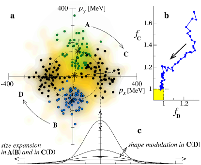
Figure 12: (a) Schematic representation of the definition of test-particle agglomerates in their initial ($A$,$B$) and final ($C$,$D$) states in momentum space in a $h^{3}$ volume. (b) Convergence of a binary nucleon-nucleon collision configuration towards a situation where Pauli blocking is strictly satisfied. The path in the plane determined by the occupancy numbers, $f_{C}$ and $f_{D}$, of the final states collects the sequence of modulations in phase-space of the test-particle clouds where the occupancy of the destination regions is iteratively optimised. (c) Examples of possible shape modulations for the packets associated with nucleons in the final state.

A remarkable advantage of the renormalised form of the residual contribution in Eq. (9) is to connect directly the fluctuation variance to the physical properties of the system, regardless the test-particle number. Such aspect has a general relevance because it makes the dynamics independent from many aspects of the numerical implementation. The dependence on $N_{\textrm{test}}$ persists on the other hand in the mean-field representation, therefore when the physical fluctuation amplitude is small, the global fluctuation phenomenology may suffer from noise effects produced by the use of a finite number of test particles in the numerical implementation of the transport equation. This remark should be kept in mind for the study of fluctuations of relatively small amplitude, like isovector fluctuations, as discussed in Sec. IV.3.

Appendix B Model parameters for nuclear matter

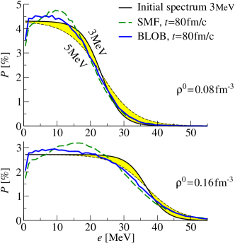
Figure 13: Energy distribution for $\rho^{0}=0.08$ (top) and $0.16$ fm^-3 (bottom), as obtained in SMF (dashed line) and BLOB (full line) calculations at $t=80$ fm/$c$. The coloured band connects the Fermi-Dirac distributions corresponding to $T=3$ and $T=5$ MeV.

In this work, for comparison purposes, both BLOB and SMF models are prepared as relying on a strictly identical implementation of the mean field, so that they differ only for the residual contribution. A simplified Skyrme-like (SKM^∗) effective interaction Guarnera1996 ; Baran2005 , where momentum-dependent terms are omitted, is employed in the propagation of the one-body distribution function, corresponding to the following definition of the potential energy per nucleon:

$$\frac{E_{\textrm{pot}}}{A}(\rho)=\frac{A}{2}u+\frac{B}{\sigma+1}u^{\sigma}+\frac{C_{\textrm{surf}}}{2\rho}(\nabla\rho)^{2}+\frac{1}{2}C_{\textrm{sym}}(\rho)u\beta^{2},$$ (38)

with $u=\rho/\rho_{\textrm{sat}}$, being $\rho_{\textrm{sat}}$ the saturation density and $\beta=(\rho_{n}-\rho_{p})/\rho$. This parameterization, with $A\!=\!-356$ MeV, $B\!=\!303$ MeV and $\sigma\!\!=\!7/6$, corresponds to a soft isoscalar equation of state with a compressibility modulus $K\!=\!200$ MeV. An additional term as a function of the density-gradient introduces a finite range of the nuclear interaction and accounts for some contribution from the zero-point motion of nucleons Guarnera1996 . $C_{\textrm{surf}}$ is related to various properties of the interaction range: the surface energy of ground-state nuclei (the best fit imposing a value of $-6/\rho_{\textrm{sat}}$ MeV fm⁵), the surface tension (light-fragment emission, in comparison to available data is better described for a smaller range given by $-7/\rho_{\textrm{sat}}$ MeV fm⁵ in BLOB), and the ultraviolet cutoff in the dispersion relation for wavelengths in the spinodal instability (larger spectrum for a smaller range) Ayik1995 . In this work, a value of $C_{\textrm{surf}}\!=\!-7/\rho_{0}$ MeV fm⁵ is chosen for the surface term. A linear (asy-stiff) density dependence of the potential part of the symmetry energy coefficient, $E_{\textrm{sym}}^{\textrm{pot}}$, is obtained by setting $C_{\textrm{sym}}(\rho)\!=\!{\textrm{constant}}\!=\!32$ MeV and a quadratic-like (asy-soft) dependence is obtained for $C_{\textrm{sym}}(\rho)\!=\!\rho_{\textrm{sat}}(482-1638\rho)$ MeV Colonna2014 .

$N_{\textrm{test}}=40$ test particles per nucleon are employed if not otherwise specified. In this work the collision term involves an isospin- and energy-dependent free nucleon-nucleon cross section with an upper cutoff at $\sigma_{\textrm{NN}}=50$ mb Napolitani2013 . In some cases, when indicated, these prescriptions may have been modified. In the SMF approach we adopt the quite short time interval of 2 fm$/c$ to inject fluctuations. In unstable conditions, like the spinodal region studied in Sec. V, the choice of a short time interval as compared to the typical growth time of unstable modes leads to convergent results on isoscalar fluctuations. We note that the growth time of unstable modes amounts to about 30 fm$/c$., quite independently of the density conditions (see Sec. V.3). Concerning isovector fluctuations, they are only induced by the finite number of test particles. Indeed, in the SMF model there are no explicit fluctuation terms injected in the isovector channel.

To simulate nuclear-matter, we prepare the system in a cubic periodic box of edge size $L=39$ fm, and we subdivide it in a lattice of cubic cells of edge size $l$ where we calculate density variances. For the sake of simplicity, we consider symmetric nuclear matter, i.e. with equal number of neutrons and protons. We initially define the system by imposing a uniform-matter effective field $U^{0}(\rho)$ whose amplitude only depends on the density considered, and a corresponding effective Hamiltonian $\epsilon(p)=h^{0}(p)=p^{2}/(2m)+U^{0}(\rho)$. Accordingly, the phase-space distribution function $f^{0}(\mathbf{p})=\{1+\mathrm{exp}[\epsilon(p)-\mu]/T\}^{-1}$, not depending on configuration space (because the system is homogeneous), is the Fermi-Dirac equilibrium distribution at the temperature $T$ and chemical potential $\mu$.

The system is initialised with a Fermi-Dirac distribution at a temperature $T=3$ MeV. As shown in Fig. 13, both SMF and BLOB transport dynamics succeed to preserve the initial distribution quite efficiently as a function of time, even though a flattening of the spectrum around an effective equilibrium temperature $T_{\textrm{eq}}$ should be accounted for, due to the fact that the Fermi statistics is not perfectly preserved. This temperature modification depends on the parameters of the calculation and is larger for larger densities.

References

- (1) J.A. Maruhn, P.-G. Reinhard, and E. Suraud, Simple Models of Many-Fermion Systems, Springer-Verlag, Berlin Heidelberg, 2010.
- (2) P. Ring and P. Schuck, The Nuclear Many-Body Problem, Springer, New York, 1980.
- (3) K. Yabana and G.F. Bertsch, Time-dependent local-density approximation in real time: Application to conjugated molecules, Int. J. of Quantum Chemistry 75, 55 (1999).
- (4) P.-G. Reinhard and E. Suraud Introduction to Cluster Dynamics”, Wiley-VCH (2004).
- (5) C. Simenel, D. Lacroix, and B. Avez, Quantum Many-Body Dynamics: Applications to Nuclear Reactions, VDM Verlag, Sarrebruck, Germany, (2010); C. Simenel, B. Avez, and D. Lacroix, Microscopic approaches for nuclear Many-Body dynamics: applications to nuclear reactions, arXiv:0806.2714, (2009).
- (6) Y. Abe, S. Ayik, P.-G. Reinhard and E. Suraud, On stochastic approaches of nuclear dynmics, Phys. Rep. 275, 49 (1996).
- (7) Ph. Chomaz, M. Colonna, and J. Randrup, Nuclear spinodal fragmentation, Phys. Rep. 389, 263 (2004).
- (8) P.-G. Reinhard, and K. Goeke, The generator coordinate method and quantised collective motion in nuclear systems, Rep. on Prog. in Phys. 50, 1 (1987).
- (9) H. Goutte, J.F. Berger, P. Casoli, and D. Gogny, Microscopic approach of fission dynamics applied to fragment kinetic energy and mass distributions in U238, Phys. Rev. C 71, 024316 (2005)
- (10) R. Balian, and M. Vénéroni, Time-Dependent Variational Principle for Predicting the Expectation Value of an Observable, Phys. Rev. Lett. 47, 1353 (1981); Correlations and fluctuations in static and dynamic mean-field approaches, Ann. Phys. 216, 351 (1992).
- (11) C. Simenel, Nuclear Quantum Many-Body Dynamics, From Collective Vibrations to Heavy-Ion Collisions, Eur. Phys. J. A 48, 152 (2012).
- (12) D. Lacroix, Large amplitude collective dynamic beyond the independent particle/quasiparticle picture, chapter in the ebook “Progress of time-dependent nuclear reaction theory”, Betham Science Publishers, honoring Prof. J. Maruhn’s 65th birthday, arXiv:1504.01499v1
- (13) Dynamics and Thermodynamics with Nuclear Degrees of Freedom, Eur. Phys. J. A 30, III (2006).
- (14) Topical issue on Nuclear Symmetry Energy, Eur. Phys. J. A 50, 9 (2014).
- (15) F. Calvayrac, P.-G. Reinhard, E. Suraud, and C.A. Ullrich, Nonlinear electron dynamics in metal clusters, Phys. Rep. 337, 493 (2000).
- (16) Th. Fennel, K.-H. Meiwes-Broer, J. Tiggesb aumker, P.-G. Reinhard, P.M. Dinh, and E. Suraud, Laser-driven nonlinear cluster dynamics, Rev. Mod. Phys. 82, 1793 (2010).
- (17) G. Chen, Nanoscale Energy Transport and Conversion: A Parallel Treatment of Electrons, Molecules, Phonons, and Photons, Oxford University Press, New York (2005).
- (18) J. Dalibard, Collisional dynamics of ultra-cold atomic gases, Proc. of the Int. School of Physics-Enrico Fermi, Course CXL, Varenna 1998.
- (19) I. Bloch, J. Dalibard, and W. Zwerger, Many-body physics with ultracold gases, Rev. Mod. Phys. 80, 885 (2008)
- (20) A.S. Schneider, C.J. Horowitz, J. Hughto, and D. K. Berry, Nuclear “pasta” formation, Phys. Rev. C 88, 065807 (2013).
- (21) C.J. Horowitz, Links between heavy ion and astrophysics, Eur. Phys. J. A 30, 303 (2006).
- (22) S.Burrello, M.Colonna, F.Matera, Phys. Rev. C 94, 012801 (2016).
- (23) F. Sébille, V. de la Mota, and S. Figerou, Probing the microscopic nuclear matter self-organization processes in the neutron star crust, Phys. Rev. C 84, 055801 (2011).
- (24) P.-G. Reinhard, and E. Suraud, Stochastic TDHF and the Boltzman-Langevin Equation, Ann. of Physics 216, 98 (1992).
- (25) E. Suraud, and P-G. Reinhard, Non-equilibrium quantum dynamics with collisional correlations, New. J. Physics 16, 063066 (2014).
- (26) N. Slama, P.-G. Reinhard, and E. Suraud, On the inclusion of collisional correlations in quantum dynamics, Annals of Physics 355, 182 (2015).
- (27) L. Lacombe, E. Suraud, P.-G. Reinhard, and P.M. Dinh Stochastic TDHF in an exactly solvable model, Annals of Phys. 373, 216 (2016).
- (28) S. Ayik and C. Grégoire, Fluctuations of single-particle density in nuclear collisions, Phys. Lett. B 212, 269 (1988).
- (29) P.-G. Reinhard and E. Suraud, The Boltzmann-Langevin Equation Derived from the Real-Time Path Formalism, Ann. of Physics 213, 204 (1992).
- (30) P. Napolitani and M. Colonna, Bifurcations in Boltzmann-Langevin One Body dynamics for fermionic systems, Phys. Lett. B 726, 382 (2013).
- (31) J. Rizzo, Ph. Chomaz, and M. Colonna, A new approach to solve the Boltzmann-Langevin equation for fermionic systems, Nucl. Phys. A806, 40 (2008).
- (32) P. Schuck and M. Tohyama, Progress in many-body theory with the equation of motion method: Time-dependent density matrix meets self-consistent RPA and applications to solvable models, Phys. Rev. B 93, 165117 (2016).
- (33) D. Lacroix and S. Ayik, Stochastic quantum dynamics beyond mean field, Eur. Phys. J. A 50, 595 (2014).
- (34) D. Lacroix, Y. Tanimura, S. Ayik, and B. Yilmaz, A simplified BBGKY hierarchy for correlated fermionic systems from a Stochastic Mean-Field approach, Eur. Phys. J. A 52, 94 (2016).
- (35) A. Bonasera, F. Gulminelli, and J. Molitoris, The Boltzmann equation at the borderline. A decade of Monte Carlo simulations of a quantum kinetic equation, Phys. Rep. 243, 1 (1994).
- (36) R. Balian, From Microphysics to Macrophysics. Methods and Appl ications of Statistical Physics. Vol1, Springer-Verlag Berlin Heidelberg GmbH (1991).
- (37) W. Cassing and A. Pfitzner, Self-consistent truncation of the BBGKY hierarchy on the two-body level, Zeit. Phys. A 342, 161 (1992).
- (38) R. Balescu, Equilibrium and Non-equilibrium Statistical Mechanics, Wiley, New York, 1976.
- (39) M. Reed and B. Simon, Methods of Modern Mathematical Physics, Vol.3 Scattering Theory, Academic Press (1979).
- (40) E. Suraud, Equations cinétiques en physique des ions lourds, 14ème Ecole Internationale Joliot-Curie de Physique Nucléaire, Maubuisson, France (1995).
- (41) C.Y. Wong, and H.H.K. Tang, Extended Time-Dependent Hartree-Fock Approximation with Particle Collisions, Phys. Rev. Lett. 40, 1070 (1978).
- (42) C.Y. Wong, and H.H.K. Tang, Dynamics of nuclear fluid. V. Extended time-dependent Hartree-Fock approximation illuminates the approach to thermal equilibrium, Phys. Rev. C 20, 1419 (1979).
- (43) D. Lacroix, S. Ayik, et Ph. Chomaz, Nuclear collective vibrations in extended mean-field theory, Progress in Particle and Nuclear Physics 52, 497 (2004).
- (44) M. Colonna, Ph. Chomaz, and J. Randrup, Linear response in stochastic mean-field theories and the onset of instabilities, Nucl. Phys. A567, 637 (1994).
- (45) S. Ayik and C. Grégoire, Transport theory of fluctuation phenomena in nuclear collisions, Nucl. Phys. A513, 187 (1990).
- (46) W. Bauer, G.F. Bertsch, and S. Das Gupta, Fluctuations and clustering in heavy-ion collisions, Phys. Rev. Lett. 58, 863 (1987).
- (47) M. Colonna, M. Di Toro, A. Guarnera, S. Maccarone, M. Zielinska-Pfabé, and H.H. Wolter, Fluctuations and dynamical instabilities in heavy-ion reactions, Nucl. Phys. A642, 449 (1998).
- (48) G.F. Burgio, Ph. Chomaz and J. Randrup, Fluctuations in nuclear dynamics, from transport theory to dynamical simulation, Nucl. Phys. A529, 157 (1991).
- (49) D. Pines and P. Nozieres, The Theory of Quantum Liquids, Benjamin, New York (1966).
- (50) E.M. Lifshitz and L.P. Pitaevskii, Statistical Physics, Part 2 – Course of Theoretical Physics, Vol. 9, Pergamon Press, Oxford (1958).
- (51) C.J Pethick and D.G. Ravenhall, Growth of Instabilities in a Normal Fermi Liquid, Ann. phys. 183, 131 ( 1988).
- (52) M. Colonna, G.F. Burgio, Ph. Chomaz, M. Di Toro, and J. Randrup, Simulating the Langevin force by simple noise in nuclear one-body dynamics, Phys. Rev. C 47, 1395 (1993).
- (53) B. Borderie and M.F. Rivet, Nuclear multifragmentation and phase transition for hot nuclei, Progr. in Part. and Nucl. Phys. (Book Series) 61, 551 (2008).
- (54) G. Tăbăcaru, B. Borderie, P. Désesquelles, M. Pârlog, M.F. Rivet, R. Bougault, B. Bouriquet, A.M. Buta, E. Galichet, B. Guiot, P. Lautesse, N. Le Neindre, L. Manduci, E. Rosato, B. Tamain, M. Vigilante, and J.P. Wieleczko, Fragment charge correlations and spinodal decomposition in finite nuclear systems, Eur. Phys. J. A 18, 103 (2003).
- (55) M. Colonna, Fluctuations and Symmetry Energy in Nuclear Fragmentation Dynamics, Phys. Rev. Lett. 110 , 042701 (2013).
- (56) M. Di Toro, V. Baran, M. Colonna, and V. Greco, Isospin in reactions, proc. of the Int. Symp. ‘̀ New Projects and Lines of Research in Nuclear Physics”, Messina 2002, World Scientific (2003).
- (57) V. Baran, M. Colonna, V. Greco, and M. Di Toro, From multifragmentation to neck fragmentation: Mass, isospin, and velocity correlations, Phys. Rep. 410, 335 (2012).
- (58) V. Baran, M. Colonna, M. Di Toro, and R. Zus, Reaction dynamics with exotic nuclei, Phys. Rev. c 85, 054611 (2005).
- (59) M. Colonna, V. Baran, M. Di Toro, and H.H. Wolter Isospin distillation with radial flow: A test of the nuclear symmetry energy, Phys. Rev. C 78, 064618 (2008).
- (60) C. Ducoin, Ph. Chomaz, and F. Gulminelli, Isospin fractionation: equilibrium versus spinodal decomposition, Nucl. Phys. A781, 407 (2007).
- (61) L.D. Landau, Oscillations in a Fermi Liquid, Sov. phys. JETP 5, 101 (1957).
- (62) M. Belkacem, V. Latora, and A. Bonasera, Dynamics of unstable matter, Phys. Lett. B 326211994.
- (63) Kalatnikov, abrikosov I.M. khalatnikov, and A.A. Abrikosov, Dispersion of sound in a fermi liquid, Sov. phys. JETP 6, 84 (1958).
- (64) W.R. Abel, A.C. Anderson, and J.C. Wheatley, Propagation of zero sound in liquid He at low temperatures, Phys. Rev. Lett. 17, 74 (1966).
- (65) V.M. Kolomietz, V.A. Plujko, and S. Shlomo, Interplay between one-body and collisional damping of collective motion in nuclei, Phys. Rev. C 54, 3014 (1996).
- (66) A.B. Larionov, M. Cabibbo, V. Baran, M. Di Toro, Strongly damped nuclear collisions: Zero or first sound?, Phys. Rev. C 61, 064614 (2000).
- (67) V.M. Kolomietz and S. Shlomo, Low density instability in a nuclear Fermi-liquid drop, Phys. Rev. C 60, 044612 (1999).
- (68) M. Colonna and Ph. Chomaz, Unstable infinite nuclear matter in stochastic mean field approach, Phys. Rev C 49, 1908 (1994).
- (69) I.Ia. Pomaranchuk, On the stability of a Fermi liquid, Sov. phys. JETP 8, 361 (1959).
- (70) M. Colonna, Ph. Chomaz, and A. Guarnera Study of multifragmentation patterns induced by spinodal instabilities, Nucl. Phys. A613, 165 (1997).
- (71) M. Baldo, G.F. Burgio, and A. Rapisarda, Dynamics of fragment formation in the nuclear spinodal region, Phys. Rev. C 51, 198 (1995).
- (72) B. Jacquot, A. Guarnera, Ph. Chomaz, and M. Colonna, Regularity and chaos in Vlasov evolution of nuclear matter, Phys. Rev. C 54, 3025 (1996).
- (73) F. Matera and A. Dellafiore, Density fluctuations and multifragmentation of nuclear matter, Phys. Rev. C 62, 044611 (2000).
- (74) S. Ayik, M. Colonna, and Ph. Chomaz, Quantal effects on growth of instabilities in nuclear matter Phys. Lett. B 353, 417 (1995).
- (75) B. Jacquot, M. Colonna, S. Ayik, and Ph. Chomaz, RPA instabilities in finite nuclei at low density, Nucl. Phys. A617, 356 (1997).
- (76) M. Colonna and Ph. Chomaz, Spinodal decomposition in nuclear molecular dynamics, Phys. Lett. B 436, 1 (1998).
- (77) W. Nörenberg, G. Papp, and P. Rozmej, Stability and instability of a hot and dilute nuclear droplet, Eur. Phys. J. A 9, 327 (2000).
- (78) S. Ayik, N. Er, O. Yilmaz, and A. Gokalp, Quantal effects on spinodal instabilities in charge asymmetric nuclear matter, Nucl. Phys. A812, 44 (2008).
- (79) P. Napolitani and M. Colonna, Frustrated fragmentation and re-aggregation in nuclei: a non-equilibrium description in spallation Phys. Rev. C 92, 034607 (2015).
- (80) F. Gagnon-Moisan et al. (INDRA Collaboration), New isospin effects in central heavy-ion collisions at Fermi energies, Phys. Rev C 86, 044617 (2012).
- (81) G. Ademard et al. (INDRA Collaboration), Isospin effects and symmetry energy studies with INDRA, Eur. Phys. J. A 50, 33 (2014).
- (82) B. Borderie et al. (INDRA Collaboration), Evidence for Spinodal Decomposition in Nuclear Multifragmentation, Phys. Rev. Lett. 86, 3252 (2001).
- (83) P. Désesquelles, Fragment size correlations in finite systems: Application to nuclear multifragmentation, Phys. Rev. C 65, 034604 (2002).
- (84) M. Colonna, P. Napolitani, and V.Baran, Mean-field instabilities and cluster formation in nuclear reactions, In preparation, arXiv:1604.03866.
- (85) N. Ashgriz and J.Y. Poo, Coalescence and separation in binary collisions of liquid drops, J. Fluid. Mech. 221, 183 (1990).
- (86) L.G. Moretto, Kin Tso, N. Colonna, and G.J. Wozniak, New Rayleigh-Taylor-like surface instability and nuclear multifragmentation, Phys. Rev. Lett. 69, 1884 (1992).
- (87) Lukasik et al. (INDRA), Dynamical effects and intermediate mass fragment production in peripheral and semicentral collisions of XeSn at 50 MeVnucleon, PRC 55, 1906 (1997).
- (88) P. Napolitani, M. Colonna, Dynamical description of heavy-ion collisions at Fermi energies, EPJ Web Conf. 117, 07008 (2016).
- (89) S. Typel, H.H. Wolter, G. Röpke, D. Blaschke, Effects of the liquid-gas phase transition and cluster formation on the symmetry energy, Eur. Phys. J. A 50, 17 (2014).
- (90) C. Kuhrts, M. Beyer, P. Danielewicz, and G. Röpke, Medium corrections in the formation of light charged particles in heavy ion reactions, Phys. Rev. C 63, 034605 (2001).
- (91) P. Danielewicz and G.F. Bertsch, Production of deuterons and pions in a transport model of energetic heavy-ion reactions, Nucl. Phys. A533, 712 (1991).
- (92) Akira Ono, Cluster production within antisymmetrized molecular dynamics, EPJ Web Conf. 122, 11001 (2016).
- (93) G.F. Bertsch and S. Das Gupta, A guide to microscopic models for intermediate energy heavy ion collisionsReview Article, Phys. Rep. 160, 189 (1988).
- (94) S. Mallik, S. Das Gupta, and G. Chaudhuri, Event simulations in a transport model for intermediate energy heavy ion collisions: Applications to multiplicity distributions, Phys. Rev. C 91, 034616 (2015).
- (95) F. Chapelle, G.F. Burgio, Ph. Chomaz, and J. Randrup, Fluctuations in nuclear dynamics: Comparison of different methods, Nucl. Phys. A540, 227 (1992).
- (96) P. Napolitani, M. Colonna, Boltzmann-Langevin One-Body dynamics for fermionic systems, EPJ Web of Conf. 31, 00027 (2012).
- (97) A.Guarnera, M.Colonna, and Ph.Chomaz, 3D stochastic mean-field simulations of the spinodal fragmentation of dilute nuclei, Phys. Lett. B 373, 267 (1996).
- (98) M. Colonna, V. Baran, and M. Di Toro, Theoretical predictions of experimental observables sensitive to the symmetry energy - Results of the SMF transport model, Eur. Phys. J. A 50, 30 (2014).