Sensitivity Properties of Intermittent Control

Abstract

The sensitivity properties of intermittent control are analysed and the conditions for a limit cycle derived theoretically and verified by simulation.

1 Introduction

Event-driven intermittent control (Gawthrop and Wang, 2009; Gawthrop et al., 2011, 2015) is a form of control where open-loop control trajectories are reset when an event, for example triggered by excessive prediction error, occurs.

Intermittent control has a long history in the physiological literature including (Craik, 1947a, b; Vince, 1948; Navas and Stark, 1968; Neilson et al., 1988; Miall et al., 1993; Bhushan and Shadmehr, 1999; Loram and Lakie, 2002; Loram et al., 2011; Gawthrop et al., 2011; van de Kamp et al., 2013b, a; Gawthrop et al., 2014). Intermittent control has also appeared in various forms in the engineering literature including (Ronco et al., 1999; Zhivoglyadov and Middleton, 2003; Montestruque and Antsaklis, 2003; Insperger, 2006; Astrom, 2008; Gawthrop and Wang, 2007, 2009; Gawthrop et al., 2012, 2015).

When applied to unstable systems, the open-loop nature of intermittent control would, at first sight, appear to be problematic. In the case of exactly-known systems, it is known (Gawthrop et al., 2014) that intermittent control of unstable systems leads to homoclinic orbits (Hirsch et al., 2012) which can be thought of as infinite-period limit cycles. In this paper, we show that if the controlled system is not exactly known, then intermittent control of unstable systems leads to limit cycles with period dependent on the discrepancy between actual and assumed system and amplitude dependent on the event trigger threshold.

The starting point of this paper is the error analysis of the intermittent control separation principle (Gawthrop and Wang, 2011). This paper extends the analysis of Gawthrop and Wang (2011) in two directions: multivariable systems and the sensitivity of intermittent control to differences between actual and the system assumed for design purposes.

§ 2 gives the background material providing the foundation for the new results in this paper. § 3 derives the error equations relevant to sensitivity analysis and derives formulae for the period and amplitude of the resultant limit cycles. § 4 gives some illustrative simulation examples and § 5 concludes the paper.

2 Background

This section summarises the information necessary to the development in § 3. Further details on the algorithm are given by Gawthrop et al. (2015) and on the error analysis by Gawthrop and Wang (2011).

2.1 Continuous Control

The analysis is based on the multivariable state-space system

$$\begin{cases}\dot{{\mathbf{x}}}(t)&=\mathbf{A}{\mathbf{x}}(t)+\mathbf{B}\mathbf{u}(t)\\ \mathbf{y}(t)&=\mathbf{C}{\mathbf{x}}(t)\end{cases}$$ (2.1)

with $n$ states represented by the $n\times 1$ vector $\mathbf{x}$, $n_{y}$ outputs represented by the $n_{y}\times 1$ vector $\mathbf{y}$ and $n_{u}$ control inputs represented by the $n_{u}\times 1$ vector $\mathbf{u}$. $\mathbf{A}$ is an $n\times n$ matrix, $\mathbf{B}$ is an $n\times n_{u}$ matrix and $\mathbf{C}$ is a $n_{y}\times n$ matrix. Following standard practice (Kwakernaak and Sivan, 1972; Goodwin et al., 2001), it is assumed that $\mathbf{A}$ and $\mathbf{B}$ are such that the system (2.1) is controllable with respect to $\mathbf{u}$ and that $\mathbf{A}$ and $\mathbf{C}$ are such that the system (2.1) is observable with respect to $\mathbf{y}$.

An observer can be designed based on the system model (2.1) to approximately deduce the system states $\mathbf{x}$ from the measured signals encapsulated in the vector $\mathbf{y}$. In particular, the observer is given by:

$$\dot{{{\mathbf{x}_{o}}}}(t) =\mathbf{A}{{\mathbf{x}_{o}}}(t)+\mathbf{B}\mathbf{u}(t)-\mathbf{L}\left({\mathbf{y}_{o}}-\mathbf{y}\right)$$ (2.2)

$$\text{where }{\mathbf{y}_{o}} =\mathbf{C}{\mathbf{x}_{o}}$$ (2.3)

The $n\times n_{y}$ matrix $\mathbf{L}$ is the observer gain matrix; it is straightforward to design $\mathbf{L}$ using a number of approaches including pole-placement and the linear-quadratic optimisation approach. The closed-loop observer dynamics are defined by the matrix $\mathbf{A}_{o}$ given by

$$\mathbf{A}_{o} =\mathbf{A}-\mathbf{L}\mathbf{C}$$ (2.4)

As discussed previously (Gawthrop et al., 2011), the resultant state-feedback gain $\mathbf{k}$ ($n\times n_{u}$) may be combined with the observer equation (2.2) to give the control signal $\mathbf{u}$ by negative feed back of the observer state as

$$\mathbf{u}(t) =-\mathbf{k}{\mathbf{x}_{o}}$$ (2.5)

The closed-loop controller dynamics are defined by the closed loop system matrix $\mathbf{A}_{c}$ given by:

$$\mathbf{A}_{c}=\mathbf{A}-\mathbf{B}\mathbf{k}$$ (2.6)

The separation principle of continuous time control is that the closed-loop stability of the closed-loop system described by Equations (2.1)– (2.6) is jointly determined by the eigenvalues of $\mathbf{A}_{c}$ and $\mathbf{A}_{o}$.

2.2 Intermittent Control

As discussed by Gawthrop et al. (2011, 2015), intermittent control makes use of three time frames:

1. continuous-time, within which the controlled system (2.1) evolves, which is denoted by $t$.

2. discrete-time points at which feedback occurs indexed by $i$. Thus, for example, the discrete-time time instants are denoted $t_{i}$ and the corresponding estimated state is ${\mathbf{x}_{o}}_{i}={\mathbf{x}_{o}}(t_{i})$. The $i$th intermittent interval $\Delta_{ol}=\Delta_{i}$ is defined as

   $$\Delta_{ol}=\Delta_{i}=t_{i+1}-t_{i}$$ (2.7)

3. intermittent-time is a continuous-time variable, denoted by $\tau$, restarting at each intermittent interval. Thus, within the $i$th intermittent interval:

   $$\tau=t-t_{i}$$ (2.8)

A lower bound $\Delta_{min}$ is imposed on each intermittent interval $\Delta_{i}>0$ (2.7):

$$\Delta_{i}>\Delta_{min}>0$$ (2.9)

The system-matched hold (SMH) is the key component of the intermittent control; the SMH state ${\mathbf{x}_{h}}$ evolves in the intermittent time frame $\tau$ as

$$\dot{{{\mathbf{x}_{h}}}}(\tau) =\mathbf{A}_{h}{\mathbf{x}_{h}}(\tau)$$ (2.10)

$$\text{where }\mathbf{A}_{h} =\mathbf{A}_{c}$$ (2.11)

$${\mathbf{x}_{h}}(0) ={\mathbf{x}_{o}}(t_{i})$$ (2.12)

where $\mathbf{A}_{c}$ is the closed-loop system matrix (2.6) and ${\mathbf{x}_{o}}$ is given by the observer equation (2.2). The hold state ${\mathbf{x}_{h}}$ replaces the observer state ${\mathbf{x}_{o}}$ in the controller equation (2.5). Other holds (where $\mathbf{A}_{h}\neq\mathbf{A}_{c}$) are possible (Gawthrop and Wang, 2007; Gawthrop and Gollee, 2012).

As discussed by Gawthrop et al. (2015), the purpose of the event detector is to generate the intermittent sample times $t_{i}$ and thus trigger feedback. Such feedback is required when the open-loop hold state ${\mathbf{x}_{h}}$ (2.10) differs significantly from the closed-loop observer state ${\mathbf{x}_{o}}$ (2.2) indicating the presence of disturbances. There are many ways to measure such a discrepancy; following Gawthrop et al. (2011), the one chosen here is to look for a quadratic function of the error $\mathbf{e}_{hp}$ exceeding a threshold $q_{t}^{2}$:

$$E =\mathbf{e}_{hp}^{T}(t)Q_{t}\mathbf{e}_{hp}(t)-q_{t}^{2}\geq 0$$ (2.13)

$$\text{where }\mathbf{e}_{hp}(t) ={\mathbf{x}_{h}}(t)-{\mathbf{x}_{o}}(t)$$ (2.14)

where $Q_{t}$ is a positive semi-definite matrix.

2.3 Analysis of Intermittent Control

As discussed by Gawthrop and Wang (2011), closed-loop IC with SMH (when the system delay is zero) and there are no disturbances or setpoint can be represented by the error system:

$$\dot{\bar{X}}(t) =\bar{\mathbf{A}}_{C}\bar{X}(t)$$ (2.15)

$$\bar{Y}(t) =\bar{\mathbf{C}}_{C}\bar{X}(t)$$ (2.16)

where:

$$\bar{Y}(t) =\begin{pmatrix}y(t)\\ u_{e}(t)\\ u(t)\end{pmatrix}$$ (2.17)

$$\text{and }\bar{X}(t) =\begin{pmatrix}x(t)\\ \tilde{\mathbf{x}}_{o}(t)\\ \tilde{\mathbf{x}}_{h}(t)\end{pmatrix}$$ (2.18)

The error system matrices are:

$$\bar{\mathbf{A}}_{C} =\begin{pmatrix}A_{c}&\boldsymbol{0}_{n\times n}&-Bk\\ \boldsymbol{0}_{n\times n}&A_{o}&\boldsymbol{0}_{n\times n}\\ \boldsymbol{0}_{n\times n}&\boldsymbol{0}_{n\times n}&A\end{pmatrix}$$ (2.19)

$$\text{and }\bar{\mathbf{C}}_{C} =\begin{pmatrix}C&\boldsymbol{0}_{1\times n}\end{pmatrix}$$ (2.20)

where $A_{c}$ is given by (2.6), $A_{o}$ by (2.4) and $A$ is the system matrix from Equation (2.1).

Using (2.15), the intersample behaviour from the sample at $t=t_{i}$ to just before the next sample at $t_{i+1}$ (denoted by ${t_{i+1}^{-}}$) is given by

$$\bar{X}({t_{i+1}^{-}}) =\bar{\Phi}_{i}\bar{X}(t_{i})$$ (2.21)

$$\text{where }\bar{\Phi}_{i} =e^{\bar{\mathbf{A}}_{C}\Delta_{i}}$$ (2.22)

Turning now to the jump behaviour at the sample times and using (2.12), the jump behaviour at $t=t_{i+1}$ is given by:

$$\bar{X}(t_{i+1}) =\bar{\mathbf{A}}_{D}\bar{X}({t_{i+1}^{-}})$$ (2.23)

$$\text{where }\bar{\mathbf{A}}_{D} =\begin{pmatrix}\boldsymbol{I}_{n\times n}&\boldsymbol{0}_{n\times n}&\boldsymbol{0}_{n\times n}\\ \boldsymbol{0}_{n\times n}&\boldsymbol{I}_{n\times n}&\boldsymbol{0}_{n\times n}\\ \boldsymbol{0}_{n\times n}&\boldsymbol{I}_{n\times n}&\boldsymbol{0}_{n\times n}\end{pmatrix}$$ (2.24)

At the sample times $t_{i}$, equation (2.12) forces the hold state and observer state to be equal; thus the third element of $\bar{X}$ is redundant. Hence Gawthrop and Wang (2011) define the vector $\bar{x}(t)$ as

$$\bar{x}(t)=\begin{pmatrix}x(t)\\ \tilde{\mathbf{x}}(t)\end{pmatrix}$$ (2.25)

It follows that, at the event times, $\bar{x}$ and $\bar{X}$ are related by:

$$\bar{x}_{i} =\mathfrak{T}\bar{X}_{i}\; \text{where }\mathfrak{T} =\begin{bmatrix}\boldsymbol{I}_{n\times n}&\boldsymbol{0}_{n\times n}&\boldsymbol{0}_{n\times n}\\ \boldsymbol{0}_{n\times n}&\boldsymbol{I}_{n\times n}&\boldsymbol{0}_{n\times n}\\ \end{bmatrix}$$ (2.26)

$$\text{and }\bar{X}_{i} =\bar{\mathfrak{T}}\bar{x}_{i}\; \text{where }\bar{\mathfrak{T}} =\begin{bmatrix}\boldsymbol{I}_{n\times n}&\boldsymbol{0}_{n\times n}\\ \boldsymbol{0}_{n\times n}&\boldsymbol{I}_{n\times n}\\ \boldsymbol{0}_{n\times n}&\boldsymbol{I}_{n\times n}\end{bmatrix}$$ (2.27)

Hence equation (2.23) can be recast in terms of $\bar{x}$ as

$$\bar{x}_{i+1} =\bar{\phi}_{i}\bar{x}_{i}$$ (2.28)

$$\text{where }\bar{\phi}_{i} =\mathfrak{T}\bar{\mathbf{A}}_{D}\bar{\Phi}_{i}\bar{\mathfrak{T}}$$ (2.29)

Gawthrop and Wang (2011) analyse Equation 2.28 for the special case of constant intermittent interval where $\bar{\phi}_{i}=\bar{\phi}$ is constant. Stability is thus dependent on the eigenvalues of $\bar{\phi}$ having magnitude less than unity.

Gawthrop and Wang (2011) discuss the effect of replacing the system-matched hold (SMH) on the error response. In contrast this note focuses on analysing the effect of incorrect system parameters on the error response: the sensitivity of the state to system error.

3 Sensitivity error analysis

This section extends the analysis of § 2.3 when the actual system is given by Equation (2.1) but the controller and observer design of § 2.1 and the hold design of § 2.2 are based on the estimated where $\mathbf{A}$, $\mathbf{B}$ and $\mathbf{C}$ are replaced by $\hat{\mathbf{A}}$, $\hat{\mathbf{B}}$ and $\hat{\mathbf{C}}$ respectively leading to a controller gain of $\hat{\mathbf{k}}$ and an observer gain of $\hat{\mathbf{L}}$. Hence the controller equation (2.5) is replaced by:

$$\mathbf{u}(t) =-\hat{\mathbf{k}}{\mathbf{x}_{o}}$$ (3.1)

the observer equation (2.2) is replaced by

$$\dot{{{\mathbf{x}_{o}}}}(t) =\hat{\mathbf{A}}{{\mathbf{x}_{o}}}(t)+\hat{\mathbf{B}}\mathbf{u}(t)-\hat{\mathbf{L}}\left({\mathbf{y}_{o}}-\mathbf{y}\right)$$ (3.2)

$$\text{where }{\mathbf{y}_{o}} =\hat{\mathbf{C}}{\mathbf{x}_{o}}$$ (3.3)

and the hold equation (2.10) is replaced by

$$\dot{{{\mathbf{x}_{h}}}}(\tau) =\hat{\mathbf{A}}_{c}{\mathbf{x}_{h}}(\tau)$$ (3.4)

$${\mathbf{x}_{h}}(0) ={\mathbf{x}_{o}}(t_{i})$$ (3.5)

$$\text{where }\hat{\mathbf{A}}_{c} =\hat{\mathbf{A}}-\hat{\mathbf{B}}\hat{\mathbf{k}}$$ (3.6)

It is assumed that the estimated system states have dimension $\hat{n}_{x}$ and are related to the actual system states by the $\hat{n}_{x}\times n_{x}$ linear transformation matrix $\hat{\mathbf{T}}$ where

$$\hat{\mathbf{x}} =\hat{\mathbf{T}}\mathbf{x}$$ (3.7)

$\mathbf{k}$ is then defined as $\mathbf{k}=\hat{\mathbf{k}}\hat{\mathbf{T}}$.

3.1 Error equations

This section derives the matrices $\bar{\mathbf{A}}_{C}$ and $\bar{\mathbf{C}}_{C}$ of Equation (2.15) corresponding to Equations (3.2) and (3.4).

Combining the actual system (2.1) with the controller equation (3.1) gives:

$$\dot{\mathbf{x}} =\mathbf{A}\mathbf{x}+\mathbf{B}\mathbf{u}=\mathbf{A}\mathbf{x}-\mathbf{B}\hat{\mathbf{k}}{\mathbf{x}_{h}}$$

$$=\mathbf{A}_{c}\mathbf{x}+\left(\mathbf{B}\mathbf{k}\mathbf{x}-\mathbf{B}\hat{\mathbf{k}}{\mathbf{x}_{h}}\right)=\mathbf{A}_{c}\mathbf{x}-\mathbf{B}\hat{\mathbf{k}}\tilde{\mathbf{x}}_{h}$$ (3.8)

$$\text{where }\tilde{\mathbf{x}}_{h} ={\mathbf{x}_{h}}-\hat{\mathbf{T}}\mathbf{x}$$ (3.9)

Combining the observer (3.2) with the actual system (2.1) gives

$${\dot{\mathbf{x}}_{o}} =\hat{\mathbf{A}}\mathbf{x}_{o}+\hat{\mathbf{B}}u-L\left(\hat{\mathbf{C}}\mathbf{x}_{o}-y\right)$$

$$=\hat{\mathbf{A}}x_{o}+\hat{\mathbf{B}}u-L\left(\hat{\mathbf{C}}x_{o}-\mathbf{C}\mathbf{x}\right)$$ (3.10)

hence the observer error equation is:

$${\dot{\tilde{\mathbf{x}}}}_{o} ={\dot{\mathbf{x}}_{o}}-\dot{\mathbf{x}}$$

$$=\left(\hat{\mathbf{A}}-\mathbf{A}\right)\mathbf{x}+\hat{\mathbf{A}}\left(x_{o}-\mathbf{x}\right)+\left(\hat{\mathbf{B}}-\mathbf{B}\right)u-\mathbf{L}\left(\hat{\mathbf{C}}\left(\mathbf{x}_{o}-\mathbf{x}\right)-\left(\hat{\mathbf{C}}-\mathbf{C}\right)\mathbf{x}\right)$$

$$=\hat{\mathbf{A}}\tilde{\mathbf{x}}_{o}+\tilde{\mathbf{A}}\mathbf{x}-\tilde{\mathbf{B}}k{\mathbf{x}_{h}}-\mathbf{L}\left(\hat{\mathbf{C}}\tilde{\mathbf{x}}_{o}-\tilde{\mathbf{C}}\mathbf{x}\right)$$

$$=\left(\hat{\mathbf{A}}-\mathbf{L}\hat{\mathbf{C}}\right)\tilde{\mathbf{x}}_{o}+\left(\tilde{\mathbf{A}}-\tilde{\mathbf{B}}k-\mathbf{L}\tilde{\mathbf{C}}\right)\mathbf{x}-\tilde{\mathbf{B}}k\tilde{\mathbf{x}}_{h}$$

$$=\tilde{\mathbf{A}}_{co}\mathbf{x}+\hat{\mathbf{A}}_{o}\tilde{\mathbf{x}}_{o}-\tilde{\mathbf{B}}k\tilde{\mathbf{x}}_{h}$$ (3.11)

$$\text{where }\tilde{\mathbf{A}}_{co} =\tilde{\mathbf{A}}-\tilde{\mathbf{B}}k-\mathbf{L}\tilde{\mathbf{C}}$$ (3.12)

$$\text{and }\hat{\mathbf{A}}_{o} =\hat{\mathbf{A}}-\mathbf{L}\hat{\mathbf{C}}$$ (3.13)

Combining the hold (3.4) with the actual system (2.1) gives

$${\dot{\tilde{\mathbf{x}}}}_{h} ={\dot{\mathbf{x}}_{h}}-\dot{\mathbf{x}}$$

$$=\hat{\mathbf{A}}_{c}\mathbf{x}_{h}-\mathbf{A}_{c}\mathbf{x}+Bk\tilde{\mathbf{x}}_{h}$$

$$=\left(\hat{\mathbf{A}}_{c}-\mathbf{A}_{c}\right)\mathbf{x}+\hat{\mathbf{A}}_{c}\left(\mathbf{x}_{h}-\mathbf{x}\right)+Bk\tilde{\mathbf{x}}_{h}$$

$$=\tilde{\mathbf{A}}_{c}\mathbf{x}+\hat{\mathbf{A}}\tilde{\mathbf{x}}_{h}-\hat{\mathbf{B}}k\tilde{\mathbf{x}}_{h}+Bk\tilde{\mathbf{x}}_{h}$$

$$=\tilde{\mathbf{A}}_{c}\mathbf{x}+\left(\hat{\mathbf{A}}-\tilde{\mathbf{B}}k\right)\tilde{\mathbf{x}}_{h}$$

$$=\tilde{\mathbf{A}}_{c}\mathbf{x}+\left(A+\tilde{\mathbf{A}}_{c}\right)\tilde{\mathbf{x}}_{h}$$ (3.14)

$$\text{where }\tilde{\mathbf{A}}_{c} =\tilde{\mathbf{A}}-\tilde{\mathbf{B}}k$$ (3.15)

Using the three error equations (3.8), (3.11) and (3.14), the matrix $\bar{\mathbf{A}}_{C}$ of Equation (2.19) is replaced by

$$\bar{\mathbf{A}}_{C} =\begin{pmatrix}\mathbf{A}_{c}&\boldsymbol{0}_{n\times n}&-\mathbf{B}k\\ \tilde{\mathbf{A}}_{co}&\hat{\mathbf{A}}_{o}&-\tilde{\mathbf{B}}k\\ \tilde{\mathbf{A}}_{c}&\boldsymbol{0}_{n\times n}&\mathbf{A}+\tilde{\mathbf{A}}_{c}\end{pmatrix}$$ (3.16)

Note that when $\hat{\mathbf{A}}=\mathbf{A}$, $\hat{\mathbf{B}}=\mathbf{B}$ and $\hat{\mathbf{C}}=\mathbf{C}$, the matrices $\tilde{\mathbf{A}}_{co}$, $\tilde{\mathbf{B}}$ and $\tilde{\mathbf{A}}_{c}$ are zero and so Equations (3.16) and (2.19) are identical.

3.2 Eigenstructure analysis

Equation (2.28) describes the evolution of the vector $\bar{x}$ (containing the system and observer error states) at the event times $t_{i}$. Through equation (2.29) for the state-transition matrix $\bar{\phi}$, this evolution is determined by the matrix $\bar{\mathbf{A}}_{C}$ of equation (3.16). As discussed by Gawthrop and Wang (2011), in the case of constant intermittent interval where $\bar{\phi}_{i}=\bar{\phi}$ is constant, the $2n$ eigenvalues $\lambda_{j}$ of $\bar{\phi}$ determine the stability of the solution of equation (2.28). As discussed in textbooks, the equation for the $j$th eigenvalue $\lambda_{j}$ is

$$\bar{\phi}v_{j}=\lambda_{j}v_{j}$$ (3.17)

where $v_{j}$ is the $j$th eigenvector. The $2n$ eigenvalue equation can be combined as

$$\bar{\phi}V =V\Lambda$$ (3.18)

$$\text{where }V =\begin{pmatrix}v_{1}&v_{2}&\dots&v_{2n}\end{pmatrix}$$ (3.19)

$$\text{and }\Delta =\begin{pmatrix}\lambda_{1}&0&\dots&0\\ 0&\lambda_{2}&\dots&0\\ \dots&\dots&\dots&\dots\\ 0&0&\dots&\lambda_{2n}\end{pmatrix}$$ (3.20)

Assuming that the eigenvalues are distinct and thus the eigenvectors $v_{j}$ are linearly independent, the $2n\times 2n$ matrix $V$ is invertible and equation (3.18) can be rewritten to give the eigendecomposition of $\bar{\phi}$

$$\bar{\phi}=V\Lambda V^{-1}$$ (3.21)

and Equation (2.28) describing the evolution of the vector $\bar{x}$ can be rewritten as:

$$\bar{\chi}_{i+1} =\Lambda\bar{\chi}_{i}$$ (3.22)

$$\text{where }\bar{\chi}(t) =V^{-1}\bar{x}(t)$$ (3.23)

Equations (3.22) and (3.23) are used in § 3.3 to determine the limit cycle period and in § 3.4 to determine the limit cycle amplitude.

3.3 Limit-Cycle Period

Gawthrop and Wang (2011) examined the stability of timed intermittent control by examining the stability of the solutions of Equation (2.28) for constant intermittent intervals $\Delta_{i}=\Delta$ when $\bar{\phi}_{i}=\bar{\phi}$. In particular, the result is based on requiring that all eigenvalues of $\bar{\phi}$ have magnitude less than one; because $\bar{\phi}$ is a function of $\Delta$, this criterion determines the range of $\Delta$ leading to stability. In contrast, this paper looks at the limit-cycle behaviour of event-driven intermittent control by examining the situation when one eigenvalue of $\bar{\phi}$ has magnitude equal to one; this criterion determines the value $\Delta_{crit}$ of $\Delta$ corresponding to a limit-cycle.

Consider the case where $\Delta=\Delta_{crit}$ is such that the $k_{1}$th eigenvalue of $\bar{\phi}$ is unity and the other eigenvalues are less than unity:

$$\lambda_{crit} =1$$ (3.24)

$$|\lambda_{k}| <1\;\forall{k\neq k_{1}}$$ (3.25)

In this case, the steady-state solution $\bar{\chi}^{ss}$ of Equation (3.22) is such that all elements are zero except for the $k_{1}$th:

$$\bar{\chi}^{ss}_{k_{1}} =\gamma$$ (3.26)

$$|\bar{\chi}^{ss}_{k}| =0\;\forall{k\neq k_{1}}$$ (3.27)

From Equation (3.23) it follows that:

$$\bar{x}^{ss} =V\bar{\chi}^{ss}=\gamma V_{k_{1}}$$ (3.28)

In other words, the steady date solution is such that at each event time, the value of $\bar{x}$ is proportional to the $k_{1}$th eigenvector of $\bar{\phi}$

$$\bar{x}(t_{i})=\bar{x}_{i}=\bar{x}^{ss}=\gamma V_{k_{1}}$$ (3.29)

Thus the state repeats at each event time: there is a limit-cycle with period $\Delta_{crit}$.

Consider the case where $\Delta=\Delta_{crit}$ is such that the $k_{1}$th eigenvalue of $\bar{\phi}$ is $-1$ and the other eigenvalues are less than unity:

$$\lambda_{crit}=\lambda_{k_{1}} =-1$$ (3.30)

$$|\lambda_{k}| <1\;\forall{k\neq k_{1}}$$ (3.31)

In this case, the above analysis gives

$$\bar{x}(t_{i})=\bar{x}_{i}=\begin{cases}\gamma V_{k_{1}}&i\emph{ even}\\ -\gamma V_{k_{1}}&i\emph{ odd}\end{cases}$$ (3.32)

The limit-cycle has a period of $2\Delta_{crit}$.

The value of $\gamma$, and the limit-cycle amplitude, are discussed in the next section.

3.4 Limit-Cycle Amplitude

The analysis of § 3.3 examines the behaviour of the intermittent controller at the event times. The inter-event behaviour is determined by Equation (2.15) which, in the $i$th interval has the solution:

$$\bar{X}(t_{i}+\tau) =e^{\bar{\mathbf{A}}_{C}\tau}\bar{X}_{i}$$ (3.33)

Using equations (2.27) and (3.29)

$$\bar{X}(t_{i}+\tau) =\gamma e^{\bar{\mathbf{A}}_{C}\tau}\bar{\mathfrak{T}}V_{k_{1}}$$ (3.34)

Hence, immediately before the next event at $t={t_{i+1}^{-}}$:

$$\bar{X}({t_{i+1}^{-}}) =\gamma e^{\bar{\mathbf{A}}_{C}\Delta_{crit}}\bar{\mathfrak{T}}V_{k_{1}}$$ (3.35)

This is the point at which the event determined by the event detector (2.13) occurs. The equation (2.14) for the event error can be rewritten in terms of $\bar{X}$ as:

$$\mathbf{e}_{hp}(t) =\mathfrak{T}_{t}\bar{X}$$ (3.36)

$$\text{where }\mathfrak{T}_{t} =\begin{pmatrix}\boldsymbol{0}_{n\times n}&-\boldsymbol{I}_{n\times n}&\boldsymbol{I}_{n\times n}\end{pmatrix}$$ (3.37)

and so the event threshold from (2.13) becomes:

$$\mathbf{e}_{hp}^{T}(t)Q_{t}\mathbf{e}_{hp}(t) =\bar{X}^{T}({t_{i+1}^{-}})\mathfrak{T}_{t}^{T}Q_{t}\mathfrak{T}_{t}\bar{X}({t_{i+1}^{-}})=q_{t}^{2}$$ (3.38)

$$\text{hence }\gamma =\frac{q_{t}}{e_{0}}$$ (3.39)

$$\text{where }e_{o}^{2} =\bar{X}_{t}^{T}\mathfrak{T}_{t}^{T}Q_{t}\mathfrak{T}_{t}\bar{X}_{t}$$ (3.40)

$$\text{and }X_{t} =e^{\bar{\mathbf{A}}_{C}\Delta_{crit}}\bar{\mathfrak{T}}V_{k_{1}}$$ (3.41)

The limit-cycle amplitude is thus proportional to the threshold parameter $q_{t}$.

4 Illustrative Simulation Examples

The following examples illustrate the theory. In each case, the system is specified by the assumed system $[\hat{\mathbf{A}}\hat{\mathbf{B}}\hat{\mathbf{C}}]$, a deviation system $[\tilde{\mathbf{A}}_{1}\tilde{\mathbf{B}}_{1}\tilde{\mathbf{C}}_{1}]$ and a parameter $\rho$ so that the actual system $[ABC]$ is given by

$$A =\hat{\mathbf{A}}-\rho\tilde{\mathbf{A}}_{1},\;B=\hat{\mathbf{B}}-\rho\tilde{\mathbf{B}}_{1},\;C=\hat{\mathbf{C}}-\rho\tilde{\mathbf{C}}_{1}$$ (4.1)

$$\text{thus }\tilde{\mathbf{A}} =\rho\tilde{\mathbf{A}}_{1},\;\tilde{\mathbf{B}}=\rho\tilde{\mathbf{B}}_{1},\;\tilde{\mathbf{C}}=\rho\tilde{\mathbf{C}}_{1},\;$$ (4.2)

4.1 Systems

There are three systems considered.

Simple.

A simple unstable system with transfer function:

$$\frac{b}{s^{2}-1}$$ (4.3)

with incorrect gain $b$.

Three-link.

The three-link example representing a standing human with hip, knee and ankle joints from Gawthrop et al. (2015) but with incorrect gain.

Neglected dynamics.

The simple system (4.3) with neglected series dynamics given by:

$$\frac{\omega_{n}^{2}}{s^{2}+2\zeta\omega_{n}+\omega_{n}^{2}}$$ (4.4)

$$\text{where }\omega_{n} =10,\;\zeta=0.5$$ (4.5)

4.2 Figure organisation

The figures are organised as

(a)

Plots of the maximum absolute value of the eigenvalues of $\bar{\phi}$ plotted against the intermittent interval $\Delta_{ol}$ (clock driven) for $\rho=0$ (no system error) and $\rho=1$. $\Delta_{crit}$ is defined as the value of $\Delta$ when the maximum absolute value rises to 1; this is indicated by the dotted lines.

(b)

The eigenvalues of $\bar{\phi}$ in the complex plane as the intermittent interval $\Delta_{ol}$ varies.

(c)

The simulated system output against time $t$ for both the intermittent controller $y$ and continuous controller $y_{c}$. The event times are indicated by dotted lines.

(d)

The system velocity $x_{1}$ is plotted against $x_{2}$ for the latter part of the simulation to show the limit-cycle. The dotted lines indicate values at event times.

(e)

The open-loop interval of the simulated system against time $t$. The predicted value $\Delta_{crit}$ is marked as the dotted line.

(f)

The eigendecomposition $\bar{\chi}$ of $\bar{x}$ (3.23) of the simulated system against time $t$ for the latter part of the simulation. Two plots are shown: $\bar{\chi}_{k_{1}}$ and the norm of the other elements of $\bar{\chi}$ together with the event times and $\gamma$ as dotted lines. Note that $\bar{\chi}_{k_{1}}=\gamma$ (or $-\gamma$) at the event times whereas the other elements of $\bar{\chi}$ are zero at the event times.

4.3 Features to note

Fig. 1

1. Simple system (4.3) with $b=0.8$.

2. The critical interval is $\Delta_{crit}=1.8~{}$\mathrm{s}$$ and the corresponding eigenvalue is at $1$.

3. The simulated system output is asymptotically periodic with period $\Delta_{crit}$. This corresponds to Equation (3.24).

4. The simulated $\Delta_{ol}$ converges to $\Delta_{crit}$.

Fig. 2

1. Simple system (4.3) with $b=1.2$.

2. The critical interval is $\Delta_{crit}=1.53~{}$\mathrm{s}$$ and the corresponding eigenvalue is at $-1$.

3. The simulated system output is asymptotically periodic with period $2\Delta_{crit}$ and mirrored half-cycles. This corresponds to Equation (3.30).

4. The simulated $\Delta_{ol}$ converges to $\Delta_{crit}$.

Fig. 3

1. Simple system (4.3) with $b=1.7$.

2. The critical interval is $\Delta_{crit}=1.1~{}$\mathrm{s}$$ and the corresponding eigenvalue is at $-1$. However, there us a further eigenvalue at $-1$.

3. The solutions does not converge to a limit-cycle.

Fig. 4

1. Three-link system with $b=0.9$.

2. The critical interval is $\Delta_{crit}=0.76~{}$\mathrm{s}$$ and the corresponding eigenvalue is at $1$.

3. The simulated system output is asymptotically periodic with period $\Delta_{crit}$.

4. The simulated $\Delta_{ol}$ converges to $\Delta_{crit}$.

5. Figure 4(d) plots the three (angular) velocities against the three (angular) positions.

Fig. 5

1. Three-link system with $b=1.1$.

2. The critical interval is $\Delta_{crit}=0.74~{}$\mathrm{s}$$ and the corresponding eigenvalue is at $-1$.

3. The simulated system output is asymptotically periodic with period $2\Delta_{crit}$ and mirrored half-cycles.

4. The simulated $\Delta_{ol}$ converges to $\Delta_{crit}$.

Fig. 6

1. Neglected dynamics system.

2. The critical interval is $\Delta_{crit}=3.6~{}$\mathrm{s}$$ and the corresponding eigenvalue is at $1$.

3. The simulated system output is asymptotically periodic with period $\Delta_{crit}$.

4. The underlying continuous-time design is unstable!

5 Conclusion

The error equations for event-driven intermittent control of multivariable systems have been extended to include discrepancies between the actual and assumed systems. The presence of limit cycles with period equal to or twice the intermittent interval have been analysed and the basic ideas illustrated by simulation.

It is believed that this work provides the foundation for adaptive intermittent control in two ways: firstly providing an analysis of behaviour before the adaptive control has converged and secondly the effect of the limit cycle in enhancing adaptation. With regard to the second point, the relay-based identification of Wang et al. (1999) seems relevant.

Further work is needed to examine the stability of the limit cycles. In particular, does the intermittent interval $\Delta_{ol}$ always converge to the predicted critical interval $\Delta_{crit}$ as illustrated in the simulations?

Experimental work is needed to verify the approach on both engineering systems and the human balance control system Loram et al. (2014).

6 Acknowledgements

The ideas for this work arose at meetings of the Intermittent Control group at Glasgow in 2016 and 2017 involving Ian Loram, Henrik Gollee, Alberto Alvarez and Ryan Cunningham.

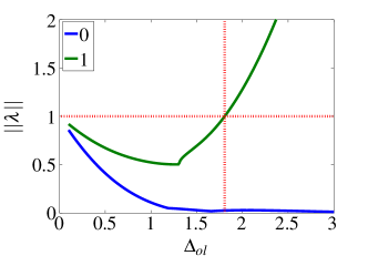
(a) Maximum eigenvalue magnitude

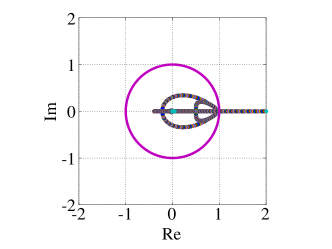
(b) Eigenvalues of $\bar{\phi}$

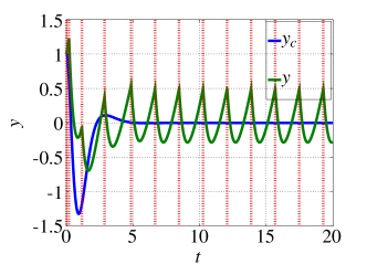
(c) Output $y$

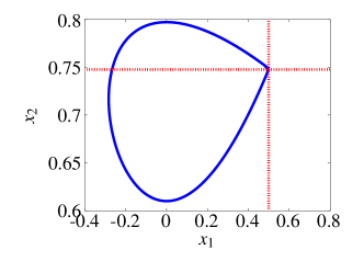
(d) Limit cycle

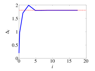
(e) OL interval $\Delta_{i}$

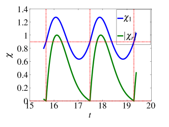
(f) Eigenvector analysis

Figure 1: Simple system: $b=0.8$. The gain is over-estimated, the critical eigenvalue $\lambda_{crit}=1$ and the period is $\Delta_{crit}=1.8$. See § 4.1 for details of the system, § 4.2 for a description of the figure layout and § 4.3 for detailed interpretation of the results.

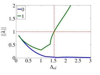
(a) Maximum eigenvalue magnitude

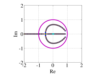
(b) Eigenvalues of $\bar{\phi}$

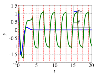
(c) Output $y$

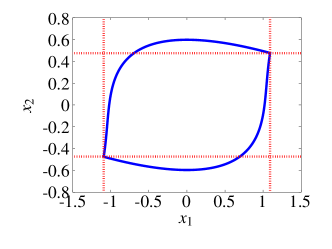
(d) Limit cycle

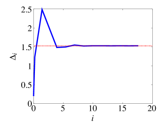
(e) OL interval $\Delta_{i}$

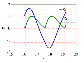
(f) Eigenvector analysis

Figure 2: Simple system: $b=1.2$. The gain is under-estimated, the critical eigenvalue $\lambda_{crit}=-1$ and the period is $2\Delta_{crit}=1.5=3$. See § 4.1 for details of the system, § 4.2 for a description of the figure layout and § 4.3 for detailed interpretation of the results.

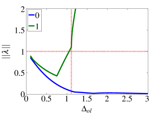
(a) Maximum eigenvalue magnitude

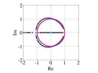
(b) Eigenvalues of $\bar{\phi}$

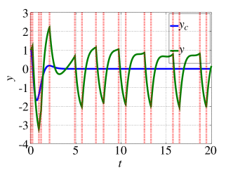
(c) Output $y$

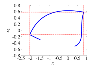
(d) Limit cycle

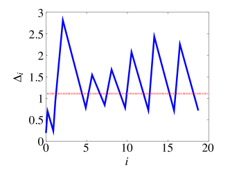
(e) OL interval $\Delta_{i}$

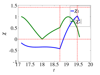
(f) Eigenvector analysis

Figure 3: Simple system: $b=1.7$. The gain is under-estimated by a large amount. When $\lambda_{k_{1}}=1$, $|\lambda_{k}|>1$ for at least one $k$ and so condition 3.24 does not hold. There is no limit cycle. See § 4.1 for details of the system, § 4.2 for a description of the figure layout and § 4.3 for detailed interpretation of the results.

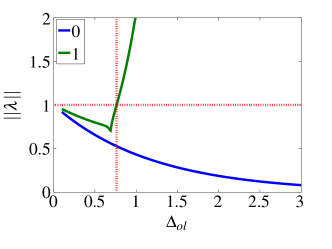
(a) Maximum eigenvalue magnitude

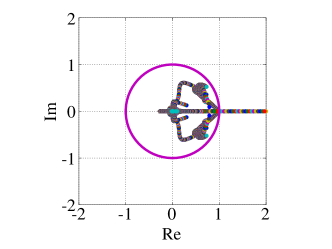
(b) Eigenvalues of $\bar{\phi}$

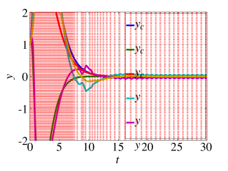
(c) Output $y$

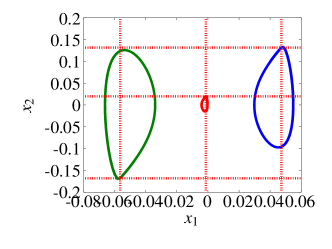
(d) Limit cycle

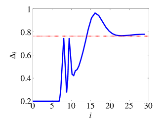
(e) OL interval $\Delta_{i}$

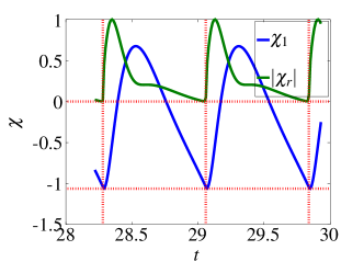
(f) Eigenvector analysis

Figure 4: Three-link system: $b=0.9$. The gain is over-estimated, the critical eigenvalue $\lambda_{crit}=1$ and the period is $\Delta_{crit}=0.76$. See § 4.1 for details of the system, § 4.2 for a description of the figure layout and § 4.3 for detailed interpretation of the results.

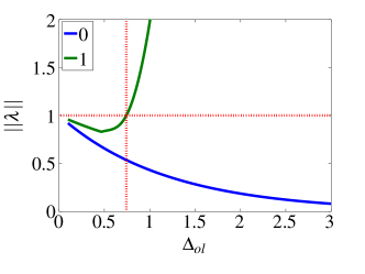
(a) Maximum eigenvalue magnitude

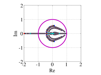
(b) Eigenvalues of $\bar{\phi}$

(c) Output $y$

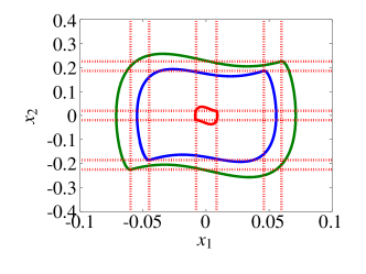
(d) Limit cycle

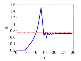
(e) OL interval $\Delta_{i}$

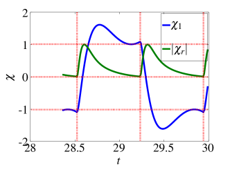
(f) Eigenvector analysis

Figure 5: Three-link system: $b=1.1$. The gain is under-estimated, the critical eigenvalue $\lambda_{crit}=-1$ and the period is $2\Delta_{crit}=1.5$. See § 4.1 for details of the system, § 4.2 for a description of the figure layout and § 4.3 for detailed interpretation of the results.

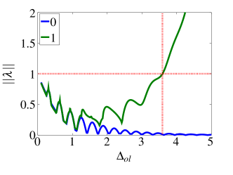
(a) Maximum eigenvalue magnitude

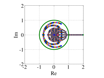
(b) Eigenvalues of $\bar{\phi}$

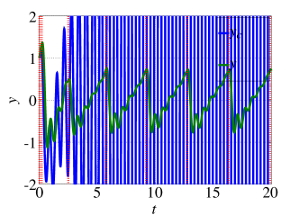
(c) Output $y$

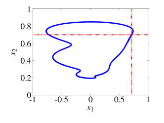
(d) Limit cycle

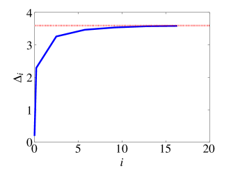
(e) OL interval $\Delta_{i}$

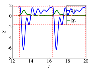
(f) Eigenvector analysis

Figure 6: System with neglected dynamics. The critical eigenvalue $\lambda_{crit}=1$ and the period is $\Delta_{crit}=3.6$. In this case, the corresponding continuous controller excites the neglected dynamics and gives an unstable response. See § 4.1 for details of the system, § 4.2 for a description of the figure layout and § 4.3 for detailed interpretation of the results.

References

Astrom (2008)
Karl J. Astrom.
Event based control.
In Alessandro Astolfi and Lorenzo Marconi, editors, Analysis
and Design of Nonlinear Control Systems, pages 127–147. Springer,
Heidelberg, 2008.
ISBN 978-3-540-74357-6.
doi:10.1007/978-3-540-74358-3.
Bhushan and Shadmehr (1999)
Nikhil Bhushan and Reza Shadmehr.
Computational nature of human adaptive control during learning of
reaching movements in force fields.
Biol. Cybern., 81(1):39–60, July 1999.
doi:10.1007/s004220050543.
Craik (1947a)
Kenneth J Craik.
Theory of human operators in control systems: Part 1, the operator as
an engineering system.
British Journal of Psychology, 38:56–61,
1947a.
doi:10.1111/j.2044-8295.1947.tb01141.x.
Craik (1947b)
Kenneth J Craik.
Theory of human operators in control systems: Part 2, man as an
element in a control system.
British Journal of Psychology, 38:142–148,
1947b.
doi:10.1111/j.2044-8295.1948.tb01149.x.