Parallel Accelerated Vector Similarity Calculations for Genomics Applications

Abstract

The surge in availability of genomic data holds promise for enabling determination of genetic causes of observed individual traits, with applications to problems such as discovery of the genetic roots of phenotypes, be they molecular phenotypes such as gene expression or metabolite concentrations, or complex phenotypes such as diseases. However, the growing sizes of these datasets and the quadratic, cubic or higher scaling characteristics of the relevant algorithms pose a serious computational challenge necessitating use of leadership scale computing. In this paper we describe a new approach to performing vector similarity metrics calculations, suitable for parallel systems equipped with graphics processing units (GPUs) or Intel Xeon Phi processors. Our primary focus is the Proportional Similarity metric applied to Genome Wide Association Studies (GWAS) and Phenome Wide Association Studies (PheWAS). We describe the implementation of the algorithms on accelerated processors, methods used for eliminating redundant calculations due to symmetries, and techniques for efficient mapping of the calculations to many-node parallel systems. Results are presented demonstrating high per-node performance and parallel scalability with rates of more than five quadrillion ($5\times 10^{15}$) elementwise comparisons achieved per second on the ORNL Titan system. In a companion paper we describe corresponding techniques applied to calculations of the Custom Correlation Coefficient for comparative genomics applications.

1 Introduction

The measurement of the similarity of pairs of vectors is a computation required in many science domains including chemistry, image processing, linguistics, ecology, document processing and genomics. To satisfy domain-specific requirements, many different similarity measures have been developed [1, 2].

The focus of the present study is the use of similarity measures in the analysis of GWAS and PheWAS results. GWAS analyses involve the statistical association of genetic variants with measured phenotypes [3]. These can be complex phenotypes such as disease states, or molecular phenotypes, such as the concentration of a particular metabolite or the expression level of a particular gene. While GWAS analyses are generally considered to involve testing association of variants with a single or limited number of phenotypes, PheWAS analyses involve testing the association of variants with a large number of different phenotypes [4]. The results of GWAS and PheWAS studies can be represented as a matrix of significant associations between variants and phenotypes, and profile vectors variants and phenotypes can be extracted from the rows and columns of this matrix. Pairwise comparisons of these vectors can allow for the discovery of phenotypes affected by similar genetic elements, or of groups of variants which affect similar phenotypes. (For example, see [5]). These studies, however, are computationally expensive, insofar as the computational work required for pairwise comparison grows as the square of the number of vectors. Even more challenging is the execution of higher-order studies which consider three or more vectors at a time—a technique required in order to discover relationships not discoverable by means of 2-way methods alone [6]—for which the computational complexity is even higher. In the past, such studies could be performed efficiently on workstations or small compute clusters. However, because of the large quantities of data involved, it is now necessary to employ large-scale high performance computing to execute scientific campaigns at the largest scales.

This paper describes advances in the development of algorithms and software to address this need. We present vector similarity measure calculation techniques for large datasets run on one of the world’s largest compute systems, scaled to thousands of compute nodes equipped with GPU accelerators. The primary contributions of this paper are implementations of similarity calculation methods which: 1) achieve high absolute performance on GPUs as a result of careful mapping of calculations to the memory hierarchy and exploiting of the highly computationally intense BLAS-3-like structure of the targeted algorithms; 2) use asynchronous internode communication, data transfers and computations to ameliorate the costs of data motion; 3) strategically arrange the computations to avoid the potential 2X-6X performance loss factor arising from the redundant calculations due to symmetry; 4) carefully parallelize the algorithms to enable near-perfect scalability to thousands of compute nodes on leadership-class systems.

In this paper we focus on the 2-way and 3-way variants of the Proportional Similarity metric, also known as the Czekanowski metric [7, 6], using an approach that is generalizable to other metrics. In the companion paper [8] we describe corresponding work on Custom Correlation Coefficient (CCC) [9] calculations with applications to comparative genomics.

Improving computational throughput for performing comparisons between pairs, triples or larger subsets of a set of vectors has been the focus of significant recent work centering around the use of parallelism, accelerated GPU or Intel Xeon Phi processing, or both. A broad overview of epistasis detection in comparative genomics including computational issues pertaining to parallelism and GPU acceleration is given in [10]. The GBOOST code, discussed in [11], is a gene-gene interaction code for 2-way studies optimized for single GPUs using encoding of gene data into bit strings with avoidance of redundant computations; [12] describes GWISFI, a single-GPU code for 2-way GWAS calculations. [13] develops a UPC++ code for gene-gene interaction studies for small numbers of GPUs and Intel Phi processors exploiting vector hardware and hardware population count instructions. [14] considers 3-way interactions on a node with 4 GPUs. [15] develops parallel tensor computation methods, structurally similar to 3-way metrics computations, with particular attention to avoiding redundant computations; however, the work does not consider GPUs or shaping of the computational regions to accommodate processors with long vector lengths. [16] discusses similarity metric calculations for chemical informatics applications on single GPUs using space filling curve methods and hardware population count instructions; it recognizes the correspondence of these calculations to BLAS-3 matrix-matrix product computations and pays close attention to optimizing memory accesses. [17] considers 2-way studies on compute clouds using MapReduce on conventional CPUs. [18] adapts existing packages to perform 2-way CPU and GPU studies and 3-way CPU studies on as many as 200 cores in parallel. [19] performs k-way GWAS studies for arbitrary k with consideration of load balancing and elimination of redundancies on a 4096-node IBM Blue Gene/Q system; results for a single GPU are also presented. [20] performs 2-way analyses on up to 126 nodes of the Intel Phi-based Stampede system (cf. [21]). [22] considers 2-way computations on thousands of compute cores with good scalability and good absolute performance on conventional CPUs. Finally, recent work in [23] considers $k$-selection similarity search methods with applications to image data with results for small numbers of GPUs; that work however focuses primarily on the $k$-selection problem for nonexhaustive inexact similarity search, a different problem from what is considered here.

The present study is to our knowledge the first work bringing together all the required ingredients for high performance 2-way and 3-way comparative genomics studies on modern leadership-class systems: use of accelerated processors at high absolute performance; optimization of calculations for use with complex memory hierarchies; elimination of redundant computations; algorithm and code design to minimize costs of I/O; and careful arrangement of communications for near-ideal scaling to many thousands of compute nodes.

The remainder of this paper is structured as follows. After describing the 2-way and 3-way Proportional Similarity metrics in Section 2, we describe the techniques used to map these methods to GPUs and other manycore accelerated processors in Section 3. Then we describe the parallelization techniques applied to these methods in Section 4, followed by implementation details in Section 5. Computational results on the 27 petaflop Oak Ridge National Laboratory (ORNL) Cray XK7 Titan system are presented in Section 6, and conclusions are given in Section 7.

2 The Proportional Similarity metric

2.1 The 2-way metric

We assume a set of $n_{v}$ vectors of length $n_{f}$ elements $\{v_{i}\}_{i=1}^{n_{v}}$ with $v_{i}\in\mathbb{R}^{n_{f}}$ and $v_{i}=\{v_{i,q}\}$. In practice, $v_{i,q}\geq 0$. Then the 2-way Proportional Similarity metric for two vectors $v_{i}$ and $v_{j}$ is $c_{2}(v_{i},v_{j})=2n_{2}(v_{i},v_{j})/d_{2}(v_{i},v_{j})$ where $d_{2}(v_{i},v_{j})={\sum_{q}v_{i,q}+v_{j,q}}={\sum_{q}v_{i,q}}+{\sum_{q}v_{j,q}}$ and $n_{2}(v_{i},v_{j})={\sum_{q}v_{i,q}\circ_{min}v_{j,q}}$. Here $a\circ_{min}b={\rm min}(a,b)$, which we define here (for reasons to be described shortly) as the “min-product,” is simply the function returning the minimum value of two scalars.

Due to symmetry of the $c_{2}()$ function with respect to its arguments, computing the metric for all pairs of distinct vectors requires computing only ${n_{v}}({n_{v}}-1)/2$ distinct values, for example, $\{c_{2}(v_{i},v_{j})\}_{i=1}^{n_{v}}{}_{j=i+1}^{n_{v}}$. Note that to perform this computation, computing the denominators $d_{2}()$ requires only $({n_{f}}-1){n_{v}}=O({n_{f}}{n_{v}})$ scalar adds, used to compute ${\sum_{q}v_{i,q}}_{i}$. The numerators $n_{2}()$ however require $({n_{f}}-1){n_{v}}({n_{v}}-1)/2$ adds and ${n_{f}}{n_{v}}({n_{v}}-1)/2$ min-product computations, thus having complexity $O({n_{f}}{n_{v}}^{2})$.

With each vector $v$ interpreted as a distribution, the Proportional Similarity metric $c_{2}(u,v)$ of two vectors is large if $u$ and $v$ have a peak at the same vector entry locations $q$ for many index values $q$ (see [24]).

2.2 The 3-way metric

The 3-way Proportional Similarity metric is defined by

$$c_{3}(v_{i},v_{j},v_{k})={3\over 2}{n_{3}(v_{i},v_{j},v_{k})\over d_{3}(v_{i},v_{j},v_{k})}$$

where $d_{3}(v_{i},v_{j},v_{k})={\sum_{q}v_{i,q}+v_{j,q}+v_{k,q}}$ and

$$n_{3}(v_{i},v_{j},v_{k})=n_{2}(v_{i},v_{j})+n_{2}(v_{i},v_{k})+n_{2}(v_{j},v_{k})-n^{\prime}_{3}(v_{i},v_{j},v_{k})$$

where $n^{\prime}_{3}(v_{i},v_{j},v_{k})={\sum_{q}v_{i,q}\circ_{min}v_{j,q}\circ_{min}v_{k,q}}$.

The function $c_{3}()$ is symmetric in its arguments, thus only ${n_{v}}({n_{v}}-1)({n_{v}}-2)/6$ distinct values need be computed, for example, $\{c_{3}(v_{i},v_{j},v_{k})\}_{i=1}^{n_{v}}{}_{j=i+1}^{n_{v}}{}_{k=j+1}^{n_{v}}$. As before, the denominators $d_{3}()$ require $({n_{f}}-1){n_{v}}=O({n_{f}}{n_{v}})$ adds. The numerators $n_{3}()$ require one computation of each of the three $n_{2}()$ values, computed as described above and used via table lookup for the first three terms of $n_{3}()$, and additionally calculation of the last term $n^{\prime}_{3}()$ requiring $({n_{f}}-1){n_{v}}({n_{v}}-1)({n_{v}}-2)/6$ adds and $2{n_{f}}{n_{v}}({n_{v}}-1)({n_{v}}-2)/6$ computations with the min-product operation, thus complexity $O({n_{f}}{n_{v}}^{3})$.

The value of the 3-way Proportional Similarity metric is large when two of the three vectors have large values at corresponding entries $q$ and even larger if all three vectors have large values at matching entries $q$.

2.3 Related metrics

The Sorenson metric is identical to the Proportional Similarity metric for the special case when $v_{i,q}\in\{0,1\}$ for all $i$, $q$. Though Sorenson metric values can be computed using methods for computing the Proportional Similarity metric, the computation can be made much faster on most processors in general use by representing vector entries as bits packed into words and operated upon using binary arithmetic, based on the coincidence of the min-product and the bitwise logical AND operations for this case.

3 Mapping to manycore processors

3.1 The 2-way metric

Since for large $n_{f}$ and $n_{v}$ the computation of the numerators $n_{2}()$ by far dominates the runtime, it is adequate to accelerate this computation only on the GPU; in the present work, all other computations are performed on the CPU.

Let $V$ represent the matrix of column vectors $V=[v_{1}v_{2}\cdots v_{n_{v}}]$. For arbitrary matrices $A=\{a_{ij}\}$ and $B=\{b_{ij}\}$, define $A\circ_{min}B$ by $(A\circ_{min}B)_{ij}=\sum_{k}a_{ik}\circ_{min}b_{kj}$. It is manifest that the desired numerators can be specified as a subset of the entries of the matrix $M=V^{T}\circ_{min}V$, for example, the strict upper triangular entries.

Note that the operation $A\circ_{min}B$ has identical computational pattern to the standard matrix-matrix product operation $A\cdot B$ for a general full matrix (GEMM), the former being defined by simply replacing the standard scalar multiplication operation $a\cdot b$ of the GEMM with the $a\circ_{min}b$ operation. This GEMM operation of the BLAS-3 standard [25] is one of the most highly optimized kernels in high performance computing and is supported by many heavily optimized libraries, typically yielding near-peak floating point operation rates for targeted processors. The approach we take here therefore is to optimize $V^{T}\circ_{min}V$ performance by adapting existing highly optimized linear algebra software to perform this operation. In what follows, we will refer to the $A\circ_{min}B$ computation as a “modified GEMM” or mGEMM operation.

On modern architectures it is of paramount importance that computations be optimized to the memory hierarchy, including registers, caches and main memory. For dense linear algebra, the complex coding effort to optimize algorithms to the memory hierarchy has already been done in the form of mathematical libraries such as the open source MAGMA library [26], which we use here. Though we do not pursue the topic here, it is likely that libraries optimized to other processor architectures, such as PLASMA [27], BLIS [28] and OpenBLAS [29], would provide similar opportunities for adapting to the mGEMM operation, in this case for conventional processors and Intel Xeon Phi.

A potential performance concern of this approach is that only half of the entries of $M=V^{T}\circ_{min}V$ are required, whereas all standard implementations of GEMM compute every entry of this matrix, resulting in potential performance loss of a factor of two. A possible remedy is to break the matrices into smaller blocks and skip computation of lower triangular blocks of $M$; however, this would still result in some performance loss since GEMM computations are most efficient at large matrix sizes. These issues are not a concern here, however; Our primary focus is the case of many compute nodes, in which case most of the time is spent in off-diagonal block computations of the form $W^{T}\circ_{min}V$ for distinct $W$ and $V$ (see below), for which there are no wasted computations. Thus the performance impact of this issue is minor.

Standard GEMMs attain high performance by spending most of the time in fused multiply-add (FMA) operations $c\leftarrow c+a\cdot b$, which are typically optimized in hardware to execute in a single clock cycle. The operation of taking the minimum of two values, however, is not so well-optimized as FMA and may in fact require a branch in execution flow, depending on the implementation. This puts a theoretical limit on the performance of Proportional Similarity metric computations that is somewhat less than that of matrix-matrix product computations. To maximize performance, here we use hardware intrinsics for taking the minimum of two values, available on recent NVIDIA GPU hardware.

Attaining high performance on a GPU-accelerated node requires overlapping transfers to and from the GPU with computations on the GPU. In this case, the mGEMM computation can be broken into blocks whose computation is overlapped with transfers. A more effective approach however is to overlap the computations $W^{T}\circ_{min}V$ of the multiple off-diagonal blocks in the parallel case with both GPU transfers and node-to-node communications in a pipelined fashion using double buffering. This is efficient since the case of many nodes requires many mGEMMs pertaining to off-diagonal blocks to be computed, as will be described below.

It is apparent that the approach described here is applicable to other vector similarity metrics that are likewise based on the accumulation of the results of a scalar operation applied to corresponding pairs of vector elements.

3.2 The 3-way metric

The calculation of 3-way metrics requires calculation of 2-way numerators as described above as well as denominators; the most expensive part for problems of significant size however is calculation of the 3-way term involving $n^{\prime}_{3}()$.

This computation could be described as “BLAS-4-like” based on its computational pattern and complexity. However, since the BLAS-3-like 2-way computation already are able to approach theoretical processor peak performance, for our purposes it will be sufficient to decompose the 3-way computation into a sequence of 2-way computations, these in turn executed as described earlier, without relying per se on the BLAS-4-like local structure of the problem.

Define the matrix $X_{j}$ such that $(X_{j})_{ik}=(V)_{ij}\circ_{min}(V)_{ik}$. The columns of $X_{j}$ are simply the elementwise min-products of the columns of $V$ with the single column $v_{j}$. Then let $B_{j}=X_{j}^{T}\circ_{min}V$. Observe $(B_{j})_{ik}=n^{\prime}_{3}(v_{i},v_{j},v_{k})$. Thus $B_{j}$ can readily be computed on GPUs using the 2-way method described earlier.

Due to symmetries it is necessary to compute only the bottom $n_{v}-j+1$ rows of $B_{j}$. Even after this optimization, some redundant calculations still remain; however, as with the 2-way case, when many GPU-enabled nodes are used most computations involve off-node blocks for which the relevant matrix entries are distinct and thus redundancy is not present. The use of only a single compute node is not the focus of performance optimization here, though in our experience even with some performance losses the methods described here may run many times faster than conventional methods at low node counts.

Since the 3-way calculation requires a sequence of GPU kernel calls corresponding to 2-way operations for the $B_{j}$ matrices described above, the calculation lends itself naturally to overlapping the transfers of data to and from the GPU with the computations on the GPU in a pipelined fashion using double buffering, thus minimizing the overhead of transfers. Furthermore, many such kernel calls can be performed without the need for intervening off-node communication in the parallel case, this being an added performance benefit resulting from the BLAS-4-like nature of the computation.

4 Multi-node parallelism

4.1 The 2-way case

We assume a large set of compute nodes, each equipped with local memory and one GPU, with interconnect programmable via MPI; this case is easily generalizable to multiple GPUs per node by assuming each GPU is associated with a single MPI rank on the node.

For the 2-way case, the primary aim is to compute the 2-D square matrix $M$ of results corresponding to the numerators $n_{2}()$ described earlier, approximately half of which are unique, describable for example by a triangular set of values (Figure 1(a)).

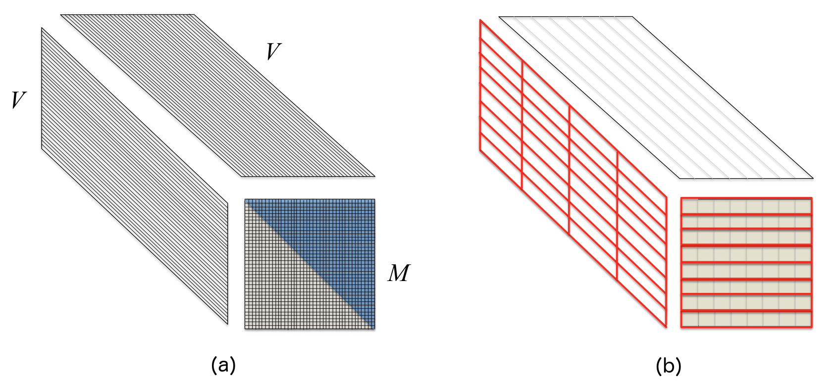
Figure 1: (a): Computational pattern of 2-way metric calculation; (b) Data decomposition for 2-way metric calculation

Considering the set of column vectors in the matrix $V$, at least two possible axes of parallelism exist. First, each vector can be split into multiple pieces and assigned to compute nodes (parallelism in vector elements: partitioning of rows of $V$). Second, a subset of the vectors can be assigned to each compute node (parallelism in vector number: partitioning of columns of $V$), with each node storing the rows of $M$ corresponding to the owned vectors (Figure 1(b)). In the present work we allow both axes of parallelism in arbitrary combination. Let $n_{pf}$ and $n_{pv}$ denote the number of nodes in the decomposition along the vector element and vector number axes, respectively, with vector elements and counts per node represented by $n_{fp}$ and $n_{vp}$.

Parallelizing along the vector elements axis requires a reduction of locally summed values along this axis to accumulate results. This typically requires $log(n_{pf})$ communication steps, each with nodes communicating $n_{vp}=n_{v}/n_{pv}$ values per node. Relying on this axis alone for parallelism is problematic for several reasons: (1) for larger values of $n_{pf}$, the logarithmic growth in communication cost with respect to node count will eventually dominate, even if communication is hidden under computation; (2) the problem sizes targeted in practice by comparative genomics problems sometimes result in small values for the vector length per node $n_{fp}=n_{f}/n_{pf}$ for large $n_{pf}$, leading to low efficiencies. For these reasons, we only consider modest amounts of parallelism along this axis. We might consider additional performance improvement from use of asynchronous reduction operations here; we will not pursue this in the present work.

Decomposing along the vector number axis necessitates an all-to-all communication. Though such operations are in general expensive, advantage can be taken here of the special structure of the problem. We formulate the computation as a sequence of parallel steps. At step $i\geq 0$, each node computes numerator values for the comparison of its own vectors with vectors stored on the node that is $i$ nodes away in the upward direction, with wraparound if needed. This process is pipelined and double-buffered, both between nodes and between each node’s CPU and GPU, so that at any parallel step, computations of numerators on the GPU, GPU transfers in each direction, communications, and computations of denominators and quotients on the CPU are all overlapped. Due to the computational intensity of the mGEMM, for sufficiently large per-node problem sizes, GPU computations will fully overlap all other operations.

This approach must be implemented so as to avoid computation of unneeded, redundant values. Using a naïve approach based on computing only the upper triangular matrix entries would result in load imbalance: some block rows assigned to compute nodes would have much less work than others and be idle for part of the computation; see Figure 2(b). The solution adopted here is to compute results associated with a block circulant-structured subset of the matrix blocks (Figure 2(c)); this subset has the properties that all unique values are represented exactly once and also each block row has the same amount of work, resulting in load balance.

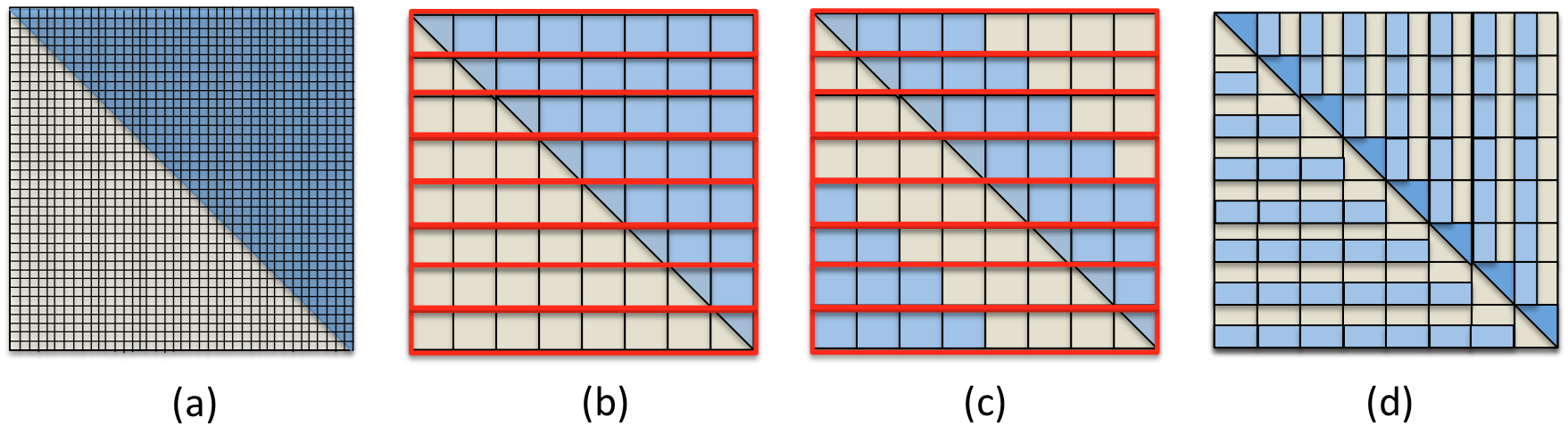
Figure 2: Load balancing for 2-way case. (a) naïve computation of upper triangular entries of result; (b) load imbalance for naïve approach; (c) load balanced method using block circulant structure of computed values; (d) alternative load balancing strategy

Past experience, e.g., with the ScaLAPACK project [30], has shown that distributed dense linear algebra based on only a 1-D decomposition of the target matrix may not provide sufficient parallelism. To generalize the above approach, we thus define an additional parallelism axis. A parameter $n_{pr}$ is chosen, and the computations of the blocks corresponding to a block row of the matrix $M$ are distributed to the $n_{pr}$ compute nodes in round-robin fashion. We thus have total internode parallelism of $n_{p}=n_{pf}n_{pv}n_{pr}$ across $n_{p}$ compute nodes. The specific decomposition is selected to tune for optimal performance for the targeted case.

The pseudocode in Algorithm 1 demonstrates the computation of metrics using the vector elements $V_{f,v}$ stored on node $(p_{f},p_{v},p_{r})$. This code, unlike the actual code, assumes for simplicity certain divisibility conditions of variables and also does not overlap communications, GPU transfers and computations.

Put $V_{f,v}$ to GPU

for $\Delta{}p_{ji}=0$ to $\lfloor n_{pv}/2\rfloor$ do

      

      if $\mod(\Delta{}p_{ji},n_{pr})=p_{r}$ then

            

            $p_{v_{s}}=mod(p_{v}-\Delta{}p_{ji},n_{pv})$; $p_{v_{r}}=mod(p_{v}+\Delta{}p_{ji},n_{pv})$

            Send $V_{f,v}$ to $(p_{f},p_{v_{s}},p_{r})$; Receive $V_{f,v_{r}}$ from $(p_{f},p_{v_{r}},p_{r})$

            Put $V_{f,v_{r}}$ to GPU; Compute $N_{f,v,v_{r}}\leftarrow V_{f,v_{r}}^{T}\circ_{min}V_{f,v}$ on GPU; Get $N_{f,v,v_{r}}$ from GPU

            Compute $N_{v,v_{r}}$ from $N_{f,v,v_{r}}$ by reduction

            Compute denominators; Compute metrics

       end if

      

end for

Algorithm 1 2-way metrics computation

4.2 The 3-way case

For the 3-way case, a 3-D cube of results must be computed, approximately 1/6 of which are unique. A tetrahedral region represents one possible selection of unique values (Figure 3(a)).

As previously, we decompose along the vector element axis and the vector number axis. For the vector element axis, we use a nonblocking reduction operation, since a sequence of mGEMM operations is readily available to overlap this reduction.

For the vector number decomposition, analogously to the 2-way case we partition the set of vectors, inducing a 1-D decomposition of the cube of results into small cube-shaped blocks arranged into “slabs,” each owned by the respective compute node (Figure 3(b)). To accomplish the all-to-all communication, a doubly nested loop is required for any given node to obtain the vectors required to compute its slab of results, analogously to the singly nested loop of the 2-way case. In particular, compute node $i$, owning vector partition $i$, must compute comparisons with vector partitions $j$ and $k$, within the nested parallel step loops over all $j$ and $k$. Each parallel step in turn entails a sequence of mGEMM operations pipelined with overlapping of transfers to and from the GPU. This inner pipeline is thus itself a component of an outer pipeline of parallel steps which overlaps the required communications of vector blocks with the mGEMM calculation pipeline.

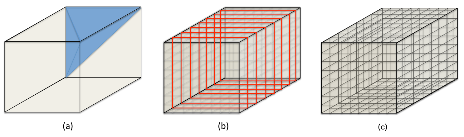
Figure 3: (a) Domain of results for 3-way metric with a representative subregion of unique values; (b) the results domain resulting from parallel decomposition across vector number; (c) induced decomposition of domain into blocks

As with the 2-way case, the redundant calculations for the 3-way case must be eliminated, to avoid potential 6X performance loss. It is unclear that the 2-way approach generalizes; we thus seek an alternative. To motivate the approach, Figure 2(d) shows for the 2-way case an alternative selection of unique values satisfying the property that not only every row but also every block has approximately the same number of computed results. Furthermore one can see by reflection across the main diagonal that all unique values are represented exactly once.

To generalize to the 3-way case we consider a partitioning of the results cube into six tetrahedra, each sharing an edge with the main diagonal of the cube (Figure 4). Onto this partitioning is superimposed the implicit tiling into blocks induced by the parallel decomposition (Figure 3(c)).

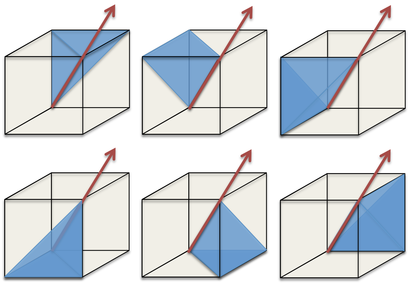
Figure 4: Decomposition of the results domain into disjoint tetrahedra

Following the approach of Figure 2(d), we now consider three types of blocks: blocks on the main diagonal of the cube (“diagonal edge blocks”), blocks on an interior face of a tetrahedron (“face blocks”), and the remaining blocks in the volume of the cube (“volume blocks”). To define the algorithm, as a first step we select for each block a strategic subset of 1/6 of the values to compute so as to cover all unique values in a load balanced fashion. We then adjust this approach to improve performance.

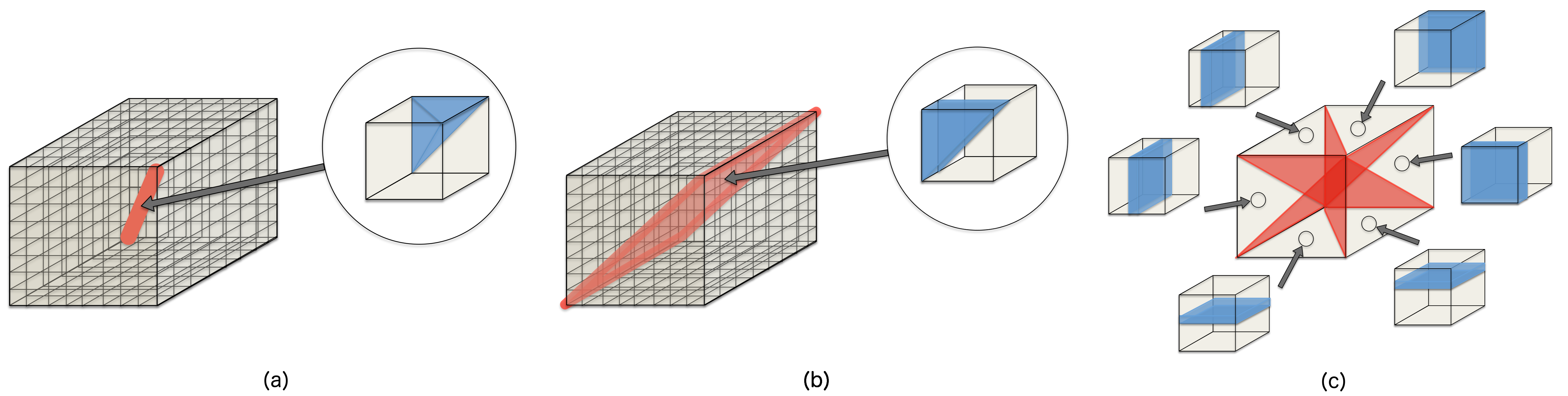
Figure 5: Compute region for main diagonal edge blocks (a), face blocks (b) and volume blocks (3)

The subset of values to compute for each block is selected as follows. For diagonal edge blocks, we select a small tetrahedron of result values (Figure 5(a)). For face blocks, one of three possible 1/3-height triangular prisms is selected, with orientation and positioning depending on the location in the cube; an example is given in Figure 5(b). Finally, for volume blocks, one of six 1/6-thickness slices of the block is selected, with placement and orientation based on location in the domain (Figure 5(c)). By a sequence of folding and reflection operations it can be shown that these combined selections are equivalent to the single large tetrahedron of values in Figure 3(a).

For significant numbers of nodes, most of the time is spent computing volume blocks. To compute a volume block, the shorter dimension of the slice is used as the GPU pipeline direction, so that the mGEMMs have maximal size and run at high efficiency.

As with the 2-way case, it is possible to extract additional parallelism. To accomplish this, the blocks computed by the doubly nested loop are round-robin distributed to a set of $n_{pr}$ compute nodes assigned to the slab. Again we have total internode parallelism of $n_{p}=n_{pf}n_{pv}n_{pr}$ across $n_{p}$ compute nodes.

In the actual implementation the above scheme is modified slightly. First, to simplify scheduling, the three diagonal planes of face blocks are folded into a single plane, so that the 1/3-height triangular prisms are replaced with a smaller set of full-height prisms; because of the structure of the computation, this change does not introduce load balancing concerns. Second, though the method described assigns an equal number of result values to each block, the work per block is not equal since volume blocks execute much more efficiently than diagonal edge and face blocks, resulting in load imbalance for high values of $n_{pr}$. To resolve this, we additionally divide diagonal edge blocks and face blocks each into six slices and distribute these slices along the $n_{pr}$ axis. As a result, each slab of the domain now has $6+6(n_{pv}-1)+(n_{pv}-1)(n_{pv}-2)=(n_{pv}+1)(n_{pv}+2)$ slices to compute. This eliminates the load balancing problem while introducing a slight load imbalance factor of $n_{pv}^{2}/(n_{pv}+1)(n_{pv}+2)$ which becomes insignificant as the node count $n_{pv}$ is made large.

An additional modification is made to improve efficiency. For the 3-way case, the number of metrics to be computed and stored can be enormous due to the algorithm’s scaling complexity. This has two tangible adverse impacts. First, nodal memory requirements constrain the problem size per node to be very small, thus reducing mGEMM efficiency. Second, the wallclock time to compute the entire complement of metrics at once may exceed the queue limit policies at some computing facilities. To remedy this, for the 3-way case we implement a staging capability: the entire run campaign for a set of metrics can be decomposed into $n_{st}$ stages, with only a single stage of results computed and stored at a time. This is implemented by dividing the GPU pipeline described earlier into $n_{st}$ parts and computing and storing the metrics for only one part at a time. This allows mGEMM sizes and thus efficiencies to be increased substantially.

As described above, the 3-way computation is composed of an inner GPU computation pipeline wrapped in an outer communication pipeline. Algorithm 2 shows pseudocode demonstrating the communication pipeline for computation of metrics using the vector elements $V_{f,v}$ stored on node $(p_{f},p_{v},p_{r})$. The pseudocode in Algorithm 3 describes the GPU pipeline computing the metrics associated with $(V_{f,v},V_{f,v_{r,j}},V_{f,v_{r,k}})$, a component of Algorithm 2. In both cases a simplified form is shown without the asynchronous behavior of the actual implementation.

Put $V_{f,v}$ to GPU; block/slice counter $s_{b}\leftarrow 0$

for $s=0$ to $5$ do

       if $mod(s_{b},n_{pr})=p_{r}$ then

            

            Compute $V_{f,v}$ denominators

            Compute metrics for block using $(V_{f,v}$, $V_{f,v}$, $V_{f,v})$

       end if

      $s_{b}\leftarrow s_{b}+1$

end for

for  $s=0$ to $5$ do

      

      for $\Delta{}p_{ji}=1$ to $n_{pv}-1$ do

            

            if $mod(s_{b},n_{pr})=p_{r}$ then

                  

                  $p_{v_{s}}=mod(p_{v}-\Delta{}p_{ji},n_{pv})$; $p_{v_{r}}=mod(p_{v}+\Delta{}p_{ji},n_{pv})$

                  Send $V_{f,v}$ to $(p_{f},p_{v_{s}},p_{r})$; Receive $V_{f,v_{r}}$ from $(p_{f},p_{v_{r}},p_{r})$

                  Put $V_{f,v_{r}}$ to GPU

                  Compute $V_{f,v_{r}}$ denominators

                  Compute metrics for block using $(V_{f,v},V_{f,v_{r}},V_{f,v_{r}})$

             end if

            

            $s_{b}\leftarrow s_{b}+1$

       end for

      

end for

for $\Delta{}p_{ki}=1$ to $n_{pv}-1$ do

      

      $p_{v_{s,k}}=mod(p_{v}-\Delta{}p_{ki},n_{pv})$; $p_{v_{r,k}}=mod(p_{v}+\Delta{}p_{ki},n_{pv})$

      Send $V_{f,v}$ to $(p_{f},p_{v_{s,k}},p_{r})$; Receive $V_{f,v_{r,k}}$ from $(p_{f},p_{v_{r,k}},p_{r})$

      Put $V_{f,v_{r,k}}$ to GPU

      Compute $V_{f,v_{r,k}}$ denominators

      for $\Delta{}p_{ji}=1$ to $n_{pv}-1$ do

            

            if $mod(s_{b},n_{pr})=p_{r}$ and $\Delta{}p_{ji}\not=\Delta{}p_{ki}$ then

                  

                  $p_{v_{s,j}}=mod(p_{v}-\Delta{}p_{ji},n_{pv})$; $p_{v_{r,j}}=mod(p_{v}+\Delta{}p_{ji},n_{pv})$

                  Send $V_{f,v}$ to $(p_{f},p_{v_{s,j}},p_{r})$; Receive $V_{f,v_{r,j}}$ from $(p_{f},p_{v_{r,j}},p_{r})$

                  Put $V_{f,v_{r,j}}$ to GPU

                  Compute $V_{f,v_{r,j}}$ denominators

                  Compute metrics for block using $(V_{f,v},V_{f,v_{r,j}},V_{f,v_{r,k}})$

             end if

            

            $s_{b}\leftarrow s_{b}+1$

       end for

      

end for

Algorithm 2 3-way metrics communication pipeline

Compute $N_{f,v_{r,j},v}\leftarrow V_{f,v_{r,j}}^{T}\circ_{min}V_{f,v}$ on GPU; Get  $N_{f,v_{r,j},v}$ from GPU; Reduce to $N_{v_{r,j},v}$

Compute $N_{f,v_{r,k},v}\leftarrow V_{f,v_{r,k}}^{T}\circ_{min}V_{f,v}$ on GPU; Get $N_{f,v_{r,k},v}$ from GPU; Reduce to $N_{v_{r,k},v}$

Compute $N_{f,v_{r,j},v_{r,k}}\leftarrow V_{f,v_{r,j}}^{T}\circ_{min}V_{f,v_{r,k}}$ on GPU; Get $N_{f,v_{r,j},v_{r,k}}$ from GPU; Reduce to $N_{v_{r,j},v_{r,k}}$

$j_{min}\leftarrow\lfloor(s_{t}+n_{st}s)(n_{v}/n_{pv})/(6n_{st})\rfloor$; $j_{max}\leftarrow\lfloor(s_{t}+1+n_{st}s)(n_{v}/n_{pv})/(6n_{st})\rfloor$

for $j=j_{min}$ to $j_{max}-1$ do

      

      Compute $X_{j}$ columns from $V_{f,v}$, $e_{j}^{T}V_{f,v_{r,j}}$; Put $X_{j}$ columns to GPU

      Compute $B_{j}$ rows; Get $B_{j}$ rows from GPU; reduce

      Compute metrics

end for

Algorithm 3 3-way metrics GPU pipeline for slice $s$ in block and stage $s_{t}$ using $(V_{f,v},V_{f,v_{r,j}},V_{f,v_{r,k}})$

5 Implementation

The algorithms described here are implemented in the CoMet parallel genomics code. This code is written in C++, compiles with the GNU compiler suite and depends on MPI, CUDA and the modified versions of the MAGMA library. GNU Make and CMake are used for build management, and googletest is used for unit testing. The clang-format source code tool from the clang compiler package is used for source code formatting, and Git is used for repository management.

OpenMP CPU threading is used to accelerate the parts of the computation that are not ported to the GPU by mapping execution to multiple CPU cores on the node; when possible, the CPU work is also hidden under the asynchronously launched GPU kernels to improve performance.

For making comparisons, each method has a reference (CPU-only) version, a (possibly optimized) CPU version, and a GPU version. A set of synthetic reference test cases is implemented for testing, designed to give the exact same bit-for-bit result for all code versions and for all parallel decompositions. Two types of synthetic problem are implemented: a version for which each vector entry is set to a randomized value, and a second version with randomized placement of entries specifically chosen so that the correctness of every result value can be verified analytically. A checksum feature using extended precision integer arithmetic computes a bit-for-bit exact checksum of computed results to check for errors when using synthetic inputs.

The code can be compiled under single or double precision. The single precision version requires less compute time and is adequate if the vector lengths are sufficiently short and the number of digits of precision required in the result is sufficiently low.

To modify MAGMA as needed for the algorithms, it is necessary to modify the two files in the MAGMA package magmablas/gemm_stencil.cuh and magmablas/gemm_stencil_defs.h. In particular, the macro definition for “fma” defining the fused multiply-add must be changed to make use of the min-product operation.

6 Computational results

6.1 Overview

Experiments are performed on the ORNL Titan Cray XK7 system. Titan is composed of 18,688 compute nodes each equipped with an AMD Interlagos 16 core CPU and an NVIDIA Kepler K20X GPU connected via a PCIe-2 bus. The K20X GPU has peak single/double precision flop rate of 3,935/1,311 GF and peak memory bandwidth of 250 GB/s. Each node contains 32 GB main memory and 6 GB GPU memory.

The software versions used are Cray OS version 5.2.82, Cray Programming Environment 2.5.5, GCC 4.9.3, MAGMA 1.6.2 and CUDA toolkit 7.5.18-1.0502.10743.2.1. For large node counts, it is in some cases necessary to set the environment variable APRUN_BALANCED_INJECTION to values such as 63 or 33 to avoid throttling of the communication network resulting from the algorithms’ communication patterns and causing performance loss.

The primary use of the code is to solve very large problems not previously solvable; thus weak scaling behavior, for which the work per node is kept roughly constant as compute node count is increased, is the primary focus.

GPU-enabled runs are executed with one MPI rank and one GPU per Titan node. Reported execution times do not include I/O and setup costs. The source code execution path for the algorithm is identical independent of the actual values contained in the input vectors; thus we expect performance for the synthetic datasets used here to be essentially identical to performance with actual genomics data.

6.2 Single GPU kernel performance

We first validate that the modified MAGMA kernel has comparable performance to the true GEMM operation. Table 1 shows results for a sample case with $n_{v}=10,240$ vectors of length $n_{f}=12,288$ elements run on a single node. Kernel times are taken from the CUDA Profiler and include kernel time only, without transfer or CPU times. GEMM achievable performance figures are taken from [31]. Though the CUDA intrinsics fmin and fminf are used in the production code, timings using the C ternary conditional operator are additionally included for comparison.

It is apparent from the results that the performance of the modified GEMM kernel is a large fraction of achievable peak GEMM rate. There is an expected degradation of performance from using a fmin or fminf hardware intrinsic combined with a scalar addition instead of FMA, insofar as FMA can execute in a single clock cycle unlike the fmin or fminf operation combined with an addition. Furthermore, the MAGMA standard GEMM on which the methods are based is not as fast as the cuBLAS GEMM. This is because the MAGMA GEMM is specifically optimized for smaller matrix sizes required by other MAGMA operations rather than the large sizes in focus here. Though the performance is high, a topic of future study is to improve the performance of this kernel, which is the ultimate performance determiner of the algorithm.

Table 1: Kernel times in seconds for single GPU case

	single	double
	precision	precision
mGEMM, c += a <b ? a : b	3.056	7.222
mGEMM, CUDA intrinsic fminf/fmin	2.602	6.484
GEMM, MAGMA	2.097	4.179
GEMM, cuBLAS	1.035	2.410
GEMM achievable peak	0.889	2.112
GEMM theoretical peak	0.655	1.966

6.3 Performance model

It is desirable to model algorithm performance in order to evaluate expected performance and also to give guidance regarding selection of tuning parameters. We assume here that mGEMM sizes are large enough to hide communications, GPU data transfers and CPU computations.

For the 2-way case, we define $\ell$, the “load,” to denote the number of blocks assigned to each node. Then the execution time of the algorithm is estimated by

$$t=t_{C}+t_{T,V}+\ell\cdot t_{G}+t_{T,M}+t_{CPU},$$

where $t_{C}$ is the time for communicating $n_{fp}n_{vp}$ vector elements per node for a parallel step, $t_{T,V}$ the time to transfer $n_{fp}n_{vp}$ vector elements to the GPU for a step, $t_{T,M}$ the time to transfer $n_{vp}^{2}$ metrics values from the GPU per step, $t_{CPU}$ the time for denominator and quotient calculations per step and $t_{G}$ the time for an mGEMM computation. The non-mGEMM times are included here to account for pipeline startup and drain, assuming the mGEMMs perfectly overlap the other operations. It is evident that maximizing $\ell$ (by limiting $n_{pr}$) makes it possible to approach peak mGEMM performance. mGEMM rates are determined empirically; the goal is to make the matrix dimensions $n_{fp}$ and $n_{vp}$ as large as possible to maximize mGEMM efficiency. This suggests for a given problem it is desirable to reduce $n_{pv}$ and $n_{pf}$ until CPU or GPU memory is filled.

For the 3-way case, we again define the load $\ell$, here representing the number of block slices computed by a node. Each slice is computed by a GPU pipeline of $(n_{vp}/6)/n_{st}$ mGEMM steps. The execution time of the algorithm is estimated by

$$t=t_{C}+t_{T,V}+\ell\cdot[(3+(n_{vp}/6)/n_{st})t_{G}+3t_{T,V}+4t_{T,M}+t_{CPU}].$$

mGEMM performance is approached by increasing $\ell$, and $n_{vp}$ and decreasing $n_{st}$, subject to memory constraints. The value of $n_{st}$ should be kept small to minimize the impact of the three 2-way metrics calculations required for each slice. As with the 2-way case, $n_{fp}$ and $n_{vp}$ should be maximized in order to maximize mGEMM performance.

6.4 GPU vs. CPU performance comparison

The following results compare performance with and without use of GPUs, to evaluate the performance advantage afforded by use of GPUs. These results use 20,000 fields on 32 compute nodes decomposed via $n_{pv}=32$ using double precision and 200,000 (2-way case) or 6,144 (3-way case) vectors. Results are shown in Table 2. The GPU version performs better than CPU by factors of 41X (2-way case) and 27X (3-way case). These figures should be compared against the roughly 10X peak flop rate ratio and 5X peak memory bandwidth ratio between GPU and CPU for each Titan node. Since the CPU code version used here is a reasonable implementation but not as heavily optimized as the GPU version, these results should not be interpreted to reflect the comparative best achievable performance by a highly optimized code for each case.

Table 2: GPU vs. CPU runtime comparisons in seconds

num way	GPU	CPU	ratio
2	76.8	3149.9	41.0
3	371.3	10067	27.1

6.5 Strong scaling results

Though the primary application of this work is weak scaling regimes, we present strong scaling results for completeness. Figure 6 shows double precision results for a fixed problem with 20,000 fields and 16,384 (2-way case) or 1,544 (3-way case) vectors. The problem is run on 2 to 64 compute nodes with various processor decompositions; the best case for each node count is shown. The parallel efficiencies at 64 nodes relative to 2 nodes are 79% (2-way) and 34% (3-way). The 3-way case is less efficient here, since the large number of metrics to be computed constrains the problem size to be smaller than what would be typically run in practice. Efficiency could be substantially increased by computing only a single stage at a time out of many compute stages, enabling larger matrix sizes; doing this here however would not be a strong scaling test in the commonly understood sense, since the the subset of elements selected for a compute stage is not independent of the processor decomposition, thus a slightly different problem would be solved in each case.

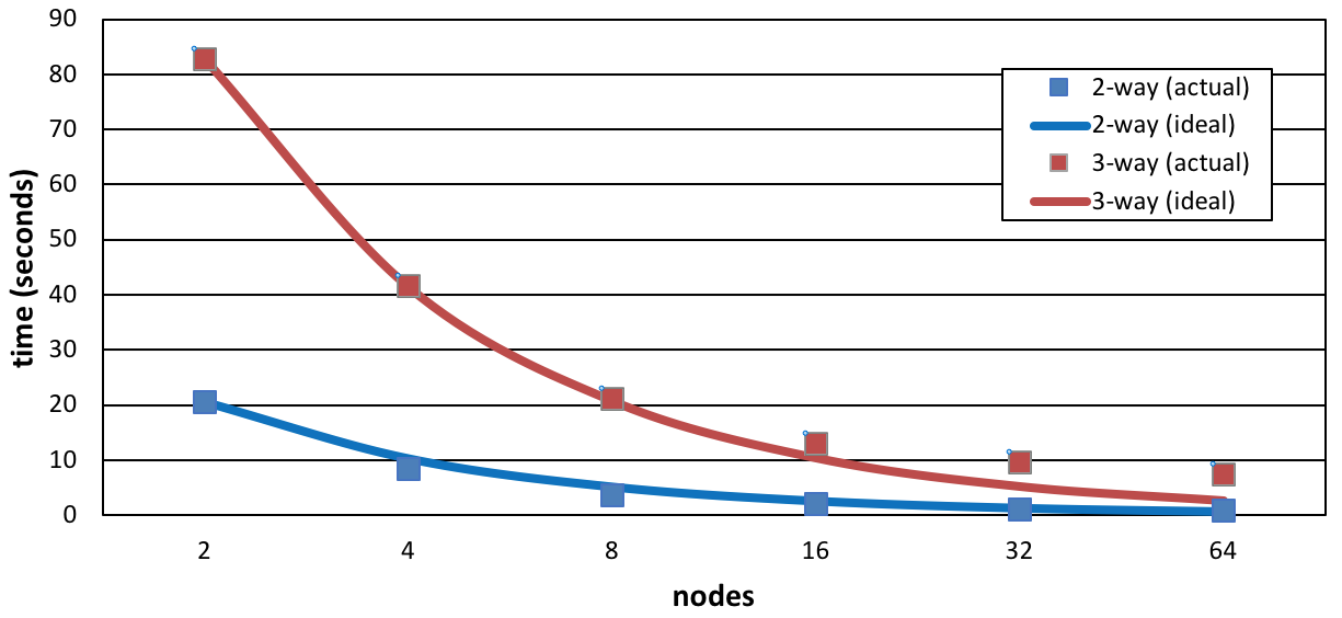
Figure 6: Proportional Similarity metric 2-way and 3-way double precision strong scaling runtimes

6.6 2-way weak scaling results

Executing a problem on $n_{p}$ nodes requires selecting tuning parameters $n_{pf}$, $n_{pv}$ and $n_{pr}$ satisfying $n_{pf}n_{pv}n_{pr}=n_{p}$. We set $n_{pf}=1$ for these experiments since actual datasets these cases are intended to emulate have modest sizes for $n_{f}$; nonetheless, experiments show that the code has very good weak scaling behavior along this axis for modest $n_{pf}$.

For fixed $n_{pv}$, setting $n_{pr}=\lceil n_{pv}/2+1\rceil$ assigns a single block to each node. We thus set $n_{pr}=\lceil\lceil n_{pv}/2+1\rceil/\ell\rceil$ where $\ell$ is the load.

Experiments are performed for up to 17,472 of Titan’s 18,688 compute nodes, or 93.5% of the system. The double precision case uses $n_{f}=5,000$ elements per vector, $n_{vp}=10,240$ vectors per node and load $\ell=13$.

Though the BLAS-3 nature of the mGEMM makes it possible to asynchronously hide communication costs for large problems, the 2-way Proportional Similarity communication costs are still challenging, in this case for example requiring messages of nearly 1/2 GB size. To maximize communication performance, we execute the 2-way runs in dedicated system mode with environment variables APRUN_BALANCED_INJECTION=96, ARMCI_DMAPP_LOCK_ON_GET=1 and ARMCI_DMAPP_LOCK_ON_PUT=1. Furthermore, following an approach previously used for optimizing parallel transpose operations [32], we apply a randomly generated mapping of the problem to compute nodes, using the MPICH_RANK_REORDER_METHOD environment variable and a specifying a random reordering by input file. Failure to use these two techniques at scale often resulted in network throttling events leading to irregular runtimes and decreased application performance by a factor of 2X or more.

Figure 7 shows weak scaling results. Timings are shown in the left graph. Though there is some loss of performance due to communication costs as the node count is increased, the performance loss is a mere 37% as the node count is increased by nearly three orders of magnitude. The right graph shows rate of operations per node, where scalar addition, scalar multiplication and scalar minimum are each counted as one operation. Since the comparison of two vector elements requires a scalar minimum and a scalar add, the value of twice the comparison rate is also shown. The values nearly match, except at low node counts for which the unneeded computations for the main diagonal block cause slight loss of performance. The implied operation rate for large cases derived from Table 1 is roughly 398 GOps/sec per node (1 GOp = $10^{9}$ operations), to which the rates in Figure 7 should be compared. The maximum comparison rate for the largest case is 1.70 petacomparisons per second; see Table 3.

In practice, the use of a random permutation of nodes might be expected to result in some performance variability based on the specific permutation used; in production, if needed one could in principle save a “good” permutation for a given node count and problem setup for subsequent reuse. However, we believe code modifications are possible which would make it unnecessary to use a random permutation of nodes: by an adjustment of the code it should be possible to recast the communication pattern as a nearest neighbor communication and then use known methods to map the communication pattern optimally to the network, see, e.g. [33]; this will be a topic of future study. In any case, as with other parallel applications, optimizing communications in a multiuser environment is challenging insofar as the network bandwidth is shared by other users and furthermore it is not always possible for a user to reserve a communication-optimal subset of nodes for job execution.

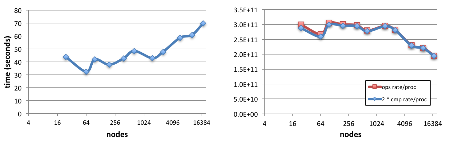
Figure 7: Proportional Similarity metric 2-way double precision weak scaling. Left: time to solution. Right: operations (add, multiply, fmin) per second, and corresponding number of unique elementwise comparisons per second per node.

The single precision test cases use $n_{f}=10,000$ elements per vector, $n_{vp}=12,288$ vectors per node and load $\ell=13$. Figure 8 shows the weak scaling results. Results are qualitatively similar to the double precision case, with rate over twice as fast, owing to the use of single precision. The performance loss is only 41% as the node count is increased by nearly three orders of magnitude. The implied operation rate for large cases derived from Table 1 is roughly 991 GOps/sec per node, to which these rates should be compared. The maximum comparison rate for the largest case is 4.29 petacomparisons per second.

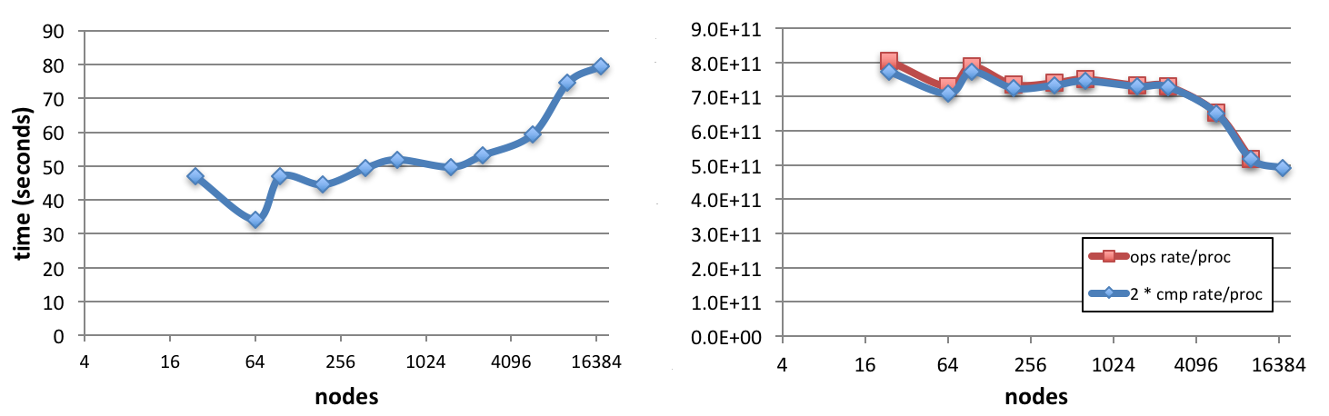
Figure 8: Proportional Similarity metric 2-way single precision weak scaling. Left: time to solution. Right: operations (add, multiply, fmin) per second, and corresponding number of unique elementwise comparisons per second per node.

Table 3: Maximum performance, 2-way Proportional Similarity metric

method	operations	comparisons
	per second	per second
double precision	$3.40\times 10^{15}$	$1.70\times 10^{15}$
single precision	$8.59\times 10^{15}$	$4.29\times 10^{15}$

6.7 3-way weak scaling results

For the 3-way case we must select $n_{pf}$, $n_{pv}$, $n_{pr}$ and additionally the stage count $n_{st}$. For load $\ell$ we set $n_{pr}=\lceil(n_{pv}+1)(n_{pv}+2)/\ell\rceil$. The stage count $n_{st}$ for best efficiency should be set to divide $n_{vp}/6$ evenly, for $n_{vp}=n_{v}/n_{pv}$ vectors per node.

The test runs are executed on up to 18,424 of Titan’s 18,688 compute nodes, or 98.6% of the system. Figure 9 shows results for the double precision case, with $n_{f}=20,000$ elements per vector and $n_{vp}=2,880$ vectors per node, computing the final stage of $n_{st}=16$ stages (pipeline depth 30), with load $\ell=6$. The left graph shows very good weak scaling behavior, with some anomalies at low node counts for which per-node performance is less efficient. The right graph shows the average operations per node primarily dominated by mGEMM costs. The rate is maintained above 300 GOps per node up to the highest node counts, a figure to be compared to the double precision GEMM rate of up to 398 GOps implied by Table 1. This is compared in the figure to twice the comparison rate per node. At lower node counts there is some disparity between the two, primarily caused by the load balancing issues described earlier, but at high node counts these two quantities approximate each other, indicating that overheads are low; the remaining disparity is mainly the result of the required 2-way computations at pipeline startup, which are counted here as part of the 3-way comparison operation.

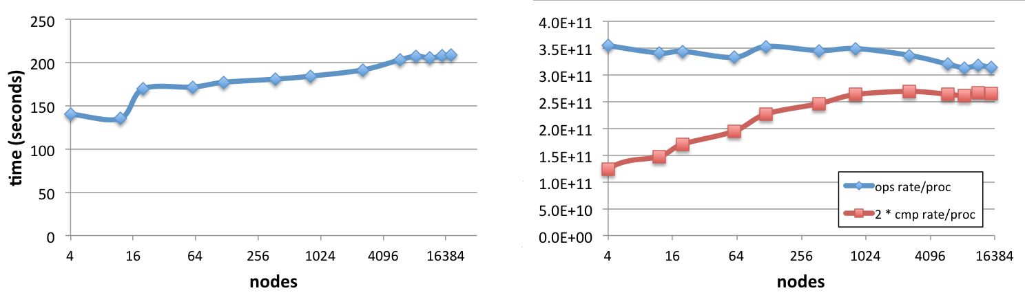
Figure 9: Proportional Similarity metric 3-way double precision weak scaling. Left: time to solution. Right: operations (add, multiply, fmin) per second, and corresponding number of unique elementwise comparisons per second per node.

Figure 10 shows corresponding results for the single precision case, with $n_{f}=20,000$ elements per vector and $n_{vp}=2,880$ vectors per node, computing the final stage of $n_{st}=16$ stages, with load $\ell=6$. The results are qualitatively similar to the double precision case, with over 2X higher performance due to increases in instruction rate and memory bandwidth.

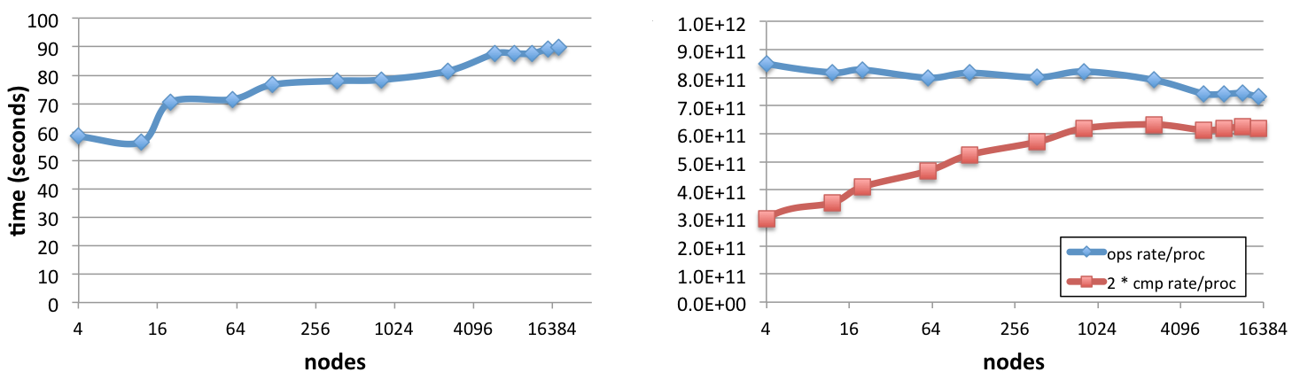
Figure 10: Proportional Similarity metric 3-way single precision weak scaling. Left: time to solution. Right: operations (add, multiply, fmin) per second, and corresponding number of unique elementwise comparisons per second per node.

Table 4 shows the maximum operation and comparison rates attained at the highest node counts, up to 2.44 petacomparisons per second (double precision) or 5.70 petacomparisons per second (single precision).

Table 4: Maximum performance, 3-way Proportional Similarity metric

method	operations	comparisons
	per second	per second
double precision	$5.75\times 10^{15}$	$2.44\times 10^{15}$
single precision	$13.40\times 10^{15}$	$5.70\times 10^{15}$

6.8 Results for a realistic sample problem

We now show results for data corresponding to an actual (i.e., nonsynthetic) problem. The input data is from a Phenome Wide Association dataset of poplar metabolites, containing all of the single nucleotide polymorphisms (SNPs) that have a significant genome wide association study (GWAS) association to one or more metabolites measured across a GWAS population of poplar trees. GWAS was performed using EMMAX [34]. This case has $n_{v}=189,625$ vectors of length $n_{f}=385$.

The runs are performed in single precision; this is satisfactory on account of the short vector lengths and modest accuracy requirements. Due to the comparatively short vector length for this dataset, it is expected that the mGEMM operations will run at less than optimal efficiency; therefore, for comparison, a synthetic problem is also run with the same dimensions and settings except that the vector length $n_{f}$ is chosen larger. All cases set $n_{pf}=1$. The input data is stored in a single column-major binary file; each compute node reads the required portion of this file. The output is written as one file per node with each metric value written as a single unsigned byte value storing roughly 2-1/2 significant figures, an adequate size for this study; all metrics are written with no thresholding. No indexing information need be written explicitly since this information can be computed formulaically offline. No further efforts are made to optimize I/O performance.

The 2-way method is run using $n_{p}=n_{pv}=30$ Titan nodes. The 3-way method is run with $n_{pv}=30$ and $n_{pr}=496$ on $n_{p}=n_{pv}\cdot n_{pr}=14,880$ Titan nodes; in this case only the last stage of $n_{st}=220$ stages is computed. Ouput is measured only for the 2-way cases. Results are given in Table 5. Performance is good for the sample case but substantially better if the vector length is longer, due to the improved mGEMM performance.

It is apparent that the high speed of the metrics calculation itself requires that careful attention be given to workflow design for scientific campaigns, specifically the handling of the large volume of generated metrics data. The trend in high performance computing system hardware is increasing compute node speed, while I/O bandwidths are growing at a much slower rate; burst buffers will increase this rate, but their storage capacities will be limited. Techniques for performing in situ analysis on the nodes before writing out results will reduce the data burden. Methods to threshold, downsample and compress data and optimize the data writing process will be important for efficient performance. Any requirements to use global methods for determining the thresholding values or other output tuning parameters will be problematic when using staging, since in this case not all of the results are available in memory at any given time to compute the needed parameters. The staging option for the 3-way case however will allow favorable opportunities for overlapping of computation and output: a stage can be computed at the same time that asynchronously the previous stage is written to disk. This strategy will require some care however, since main memory bandwidth is required for the output as well as for the data transfers to and from the GPU during compute and also for communication; these competing operations will need to be carefully scheduled in order to avoid resource contention.

Table 5: Sample problem timings in seconds (unoptimized I/O)

num way	$n_{f}$	input	metrics comp	output	comparison
		time	time	time	rate / node
2	385	.06	1.85	24.78	125e9
2	20,000	—	28.86	24.79	415e9
3	385	13.89	15.38	—	54e9
3	5,000	—	33.37	—	321e9

6.9 Comparison with other work

We now compare against results reported in the literature as described in Section 1. We consider the most relevant comparable work we are aware of as of this writing. Table 6 shows comparisons per second for alternative methods and implementations. Unfortunately, it is difficult to make rigorous comparisons when architectures and algorithms are significantly different and source code for the methods is not available or is not easily ported and tuned to a single common architecture for comparison. Furthermore, most reported results in the literature for vector similarity for genomics applications represent input values as bits rather than full floating point values. This makes comparisons tenuous insofar as manipulating many binary values packed into a word is disproportionately much faster than operating on floating point numbers. With these caveats in mind we report element comparisons per second in Table 6, whether an element is a single bit, a string of 2 or 3 bits, or a floating point number. Also as a rough measure of this performance normalized against hardware capability, a normalized performance ratio is calculated by normalizing the (absolute) comparison rate against the floating point rate of the respective hardware. For newer hardware, the double precision peak rate is used; for older GPUs with weak or nonexistent double precision support, single precision is used.

We consider first the raw number of comparisons per second. Table 6 demonstrates that the CoMet code used in the present work gives several orders of magnitude higher absolute performance, as measured in comparisons per second, far beyond the demonstrated capability of any other code. Furthermore, the 3-way method’s normalized performance ratio is as high as 5X higher than that of any other 3-way implementation shown.

The normalized performance ratio of CoMet is within the general range of performance ratios of the other methods. Also, the CoMet 2-way single precision method’s rate is within about a factor of four of the best performing 2-way GWAS method. This should be considered a strong result, insofar as the bitwise GWAS methods operate on 2-bit or 3-bit values, disproportionately easier since they are less than one-tenth the size of the 32 bit floating point values operated on by the current code. Also, pointing back to Table 1, CoMet code performance is already approaching peak available performance of the underlying hardware; thus we believe that in a fair apples-to-apples comparison the present code would rank well. Finally, the performance of [16] is exceptionally high since the codes operate on single bit values and the CPU code exploits native high performance features of that processor model.

Table 6: Comparisons to related work

code	problem	node config	nodes	GFlop rate	cmp/sec	norm
			used		($\times 10^{9}$)	perf
[16]	2-way 1-bit	1 Intel Core i7-920	1	42.56 DP	222	5.216
GBOOST[11]	2-way GWAS	1 NVIDIA GTX 285	1	1062.72 SP	64.08	.060
GWISFI[12]	2-way GWAS	1 NVIDIA GTX 470	1	1088.6 SP	767	.705
[19]	2-way GWAS	1 NVIDIA GTX 470	1	1088.6 SP	649	.596
[16]	2-way 1-bit	1 NVIDIA GTX 480	1	1345 SP	1185	.881
[19]	2-way GWAS	IBM Blue Gene/Q	4096	839e3 DP	2520	.003
epiSNP[20]	2-way GWAS	2 Intel Xeon Phi SE10P	126	271e3 DP	1593	.006
[13]	2-way GWAS	2 NVIDIA K20m +	1	3360.56 DP	1053	.313
		1 Intel Xeon Phi 5110P
CoMet	2-way PS SP	1 NVIDIA K20X	17472	25.3e6 DP	4.290e6	.169
CoMet	2-way PS DP	1 NVIDIA K20X	17472	25.3e6 DP	1.700e6	.067
GPU3SNP[14]	3-way GWAS	4 NVIDIA GTX Titan	1	6000 DP	264.7	.044
CoMet	3-way PS SP	1 NVIDIA K20X	18424	26.7e6 DP	5.700e6	.213
CoMet	3-way PS DP	1 NVIDIA K20X	18424	26.7e6 DP	2.440e6	.091

7 Conclusions

We have defined a new set of algorithm implementations for computing 2-way and 3-way vector comparison metrics on leadership class systems, showing performance of up to five quadrillion vector element comparisons per second. To our knowledge this is the first computation of its kind ever performed at this scale, demonstrating the capability to perform simulations that were until recently considered far beyond what is possible, enabling new kinds of science in GWAS and PheWAS to be done.

Future work will include investigation of additional code performance improvements—for example, improved mGEMM performance and lessening of overheads by additional code tuning. We anticipate the methods described here will be directly portable to alternative processor architectures such as Intel Xeon Phi. We will also examine implementation of higher order comparison methods. Use of these methods will require careful engineering of computational science workflows in such a way that the entire workflow is well optimized for scientific discovery.

References

References

- [1] S.-H. Cha, Comprehensive Survey on Distance/Similarity Measures between Probability Density Functions, International Journal of Mathematical Models and Methods in Applied Sciences 1 (4), , http://arabic-icr.googlecode.com/git/Papers/Comprehensive%20Survey%20on%20Distance-Similarity.pdf. [Online; accessed 1-March-2016].
- [2] D. A. Weighill, D. Jacobson, Network Metamodeling: Effect of Correlation Metric Choice on Phylogenomic and Transcriptomic Network Topology, Advances in Biochemical Engineering/Biotechnology.
- [3] N. Solovieff, C. Cotsapas, P. H. Lee, S. M. Purcell, J. W. Smoller, Pleiotropy in complex traits: challenges and strategies, Nature Reviews Genetics 14 (7) (2013) 483–495.
- [4] S. Pendergrass, K. Brown-Gentry, S. Dudek, E. Torstenson, J. Ambite, C. Avery, S. Buyske, C. Cai, M. Fesinmeyer, C. Haiman, et al., The use of phenome-wide association studies (PheWAS) for exploration of novel genotype-phenotype relationships and pleiotropy discovery, Genetic epidemiology 35 (5) (2011) 410–422.
- [5] S. Bolormaa, J. E. Pryce, A. Reverter, Y. Zhang, W. Barendse, K. Kemper, B. Tier, K. Savin, B. J. Hayes, M. E. Goddard, A Multi-Trait, Meta-analysis for Detecting Pleiotropic Polymorphisms for Stature, Fatness and Reproduction in Beef Cattle, PLoS Genet 10 (3) (2014) e1004198.
- [6] D. A. Weighill, D. A. Jacobson, 3-way Networks: Application of Hypergraphs for Modelling Increased Complexity in Comparative Genomics, PLoS Computational Biology 11 (3), , http://journals.plos.org/ploscompbiol/article?id=10.1371/journal.pcbi.1004079. [Online; accessed 1-March-2016].
- [7] J. R. Bray, J. T. Curtis, An Ordination of the Upland Forest Communities of Southern Wisconsin, Ecological Monographs 27 (4), , http://www.geobotany.org/teaching/biol474/journals/Bray1957v27n4.pdf. [Online; accessed 1-March-2016].
- [8] W. Joubert, J. Nance, S. Climer, D. Weighill, D. Jacobson, Parallel Accelerated Custom Correlation Coefficient Calculations for Genomics Applications, Parallel Computing, submitted.
- [9] S. Climer, W. Yang, L. de las Fuentes, V. G. Davila-Roman, C. C. Gu, A Custom Correlation Coefficient (CCC) Approach for Fast Identification of Multi-SNP Association Patterns in Genome-Wide SNPs Data, Genetic Epidemiology 38 (7), , http://www.ncbi.nlm.nih.gov/pubmed/25168954. [Online; accessed 1-March-2016].
- [10] W.-H. Wei, G. Hemani, C. S. Haley, Detecting epistasis in human complex traits, Nature Reviews Genetics, http://www.nature.com/nrg/journal/v15/n11/full/nrg3747.html. [Online; accessed 11-October-2016].
-
[11]
L. S. Yung, C. Yang, X. Wan, W. Yu,