Spontaneous breakdown of charge in the MSSM and in the NMSSM: Possibilities and Implications

Abstract

We study the possibilities and the implications of a spontaneous breakdown of charge in the MSSM and in the $Z_{3}$-symmetric NMSSM. The breakdown is triggered by the charged states of the Higgs doublets acquiring vacuum expectation values. In the MSSM, it is known that the presence of a charge conserving minimum for the tree-level Higgs potential precludes a deeper (global) charge-breaking minimum. We find that the inclusion of radiative correction to the potential does not alter the situation while a deeper charge-conserving minimum could arise, albeit with no major practical consequences. In the NMSSM scenario, a charge-breaking global minimum, with or without an accompanying charge-conserving deeper minimum, could appear even with the tree-level Higgs potential thanks to the presence of a charge-neutral scalar state which transforms as a singlet under the Standard Model gauge group. Use of the NMSSM Higgs potential that includes both quantum and thermal corrections and the requirement of a viable (stable or long-lived) vacuum that breaks the electroweak symmetry, along with its compatibility with the latest Higgs data, lead to nontrivial constraints on the NMSSM parameter space.

1 Introduction

In scenarios with two Higgs doublets, a spontaneous breakdown of charge could occur when the charged components of the doublets acquire vacuum expectation values (vev). The desired (electroweak) symmetry breaking (DSB) vacuum conserves charge. In the presence of a spontaneous breakdown of charge, the DSB vacuum can be, in general, accompanied by both charge-conserving (CC) and charge-breaking (CB) minima Ferreira:2004yd . Under such a circumstance, a viable DSB vacuum is required to be either the global minimum of the Higgs potential or, in case it is not (a metastable DSB vacuum), it has to have a slow enough tunneling to the deeper CC or the CB minimum (the panic vacuum) thus becoming cosmologically long-lived.

Crucially enough, for two Higgs doublet models (2HDM), it has been shown rigorously that if the tree-level Higgs potential is attributed with a CC minimum, it has to be the deepest (global) minimum Ferreira:2004yd ; Barroso:2005sm . In other words, if the potential has got a CB minimum, it can only be shallower than the CC minimum. Such a CB minimum is also found to be invariably a saddle point Barroso:2005sm . Hence, if the CC minimum now happens to be the DSB vacuum, this would be absolutely stable against tunneling to the CB minimum. However, in the absence of a CB minimum, if there is another CC minimum apart from the DSB one, it is to be seen if the latter still remains to be the deepest minimum. This is since there is no general argument to prove or refute such a possibility Barroso:2005sm . Detailed studies of (meta)stability of the DSB vacuum in generic 2HDM (including multi-HDM) had been taken up earlier in references Maniatis:2006fs ; Barroso:2013awa (Barroso:2006pa ) and, more recently, in reference Staub:2017ktc in the context of 2HDM. In any case, if the DSB vacuum ceases to be the global minimum, one needs to check if it is long-lived enough so as to become viable.

Presence of additional scalars in scenarios beyond the Standard Model (SM) invariably gives rise to more complicated scalar potentials. In some such scenarios, one could thus naturally expect the occurrence of potential-minima deeper than the DSB vacuum at the tree-level itself. These may destabilize the latter as it may undergo quantum tunneling to a deeper vacuum. Requiring a stable DSB vacuum, thus, puts stringent theoretical restrictions on the parameter space of the scenario. In this context, appearance of spontaneous charge and color breaking (CCB) minima in various supersymmetric (SUSY) scenarios (as the scalar partners of the SM quarks (squarks) and the leptons (sleptons) acquire vev) and its implications for the stability of the DSB vacuum have been a much-studied area AlvarezGaume:1983gj ; Gunion:1987qv ; Casas:1995pd ; Strumia:1996pr ; Baer:1996jn ; Abel:1998cc ; Abel:1998wr ; Chowdhury:2013dka ; Blinov:2013fta ; Hollik:2015pra ; Hollik:2016dcm . These general studies are only recently been followed up and improved Camargo-Molina:2014pwa ; Chattopadhyay:2014gfa within the framework of the Minimal Supersymmetric Standard Model (MSSM) by precise treatments of several indispensable issues thus yielding a more conclusive picture.

Interestingly enough, inclusion of even a singlet scalar excitation (in an otherwise 2HDM scenario) could turn the scalar potential rather nontrivial. Early studies Ellwanger:1996gw ; Ellwanger:1999bv ; Kanehata:2011ei ; Kobayashi:2012xv in the framework of the Next-to-Minimal Supersymmetric Standard Model (NMSSM) (which is endowed with an additional scalar which is electrically neutral and which transforms as a singlet under the SM gauge group), though restricted in their scopes, uncovered some of the salient features of such a potential in reference to the stability of the DSB vacuum. A recent in-depth study Beuria:2016cdk has not only lent phenomenological credence to some of those earlier observations but has also extended the ambit of such studies by revealing interesting, new aspects and by detailed profiling of the vacua that appear.

In contrast, the possibility and the implications of a spontaneous breakdown of charge had attracted less attention. It may, however, be noted that such a possibility had earlier been pointed out Ellwanger:2009dp in the context of the NMSSM. Subsequently, it has been studied how such a CB minimum could appear in the so-called Next-to-Minimal 2HDM (N2HDM) wittbrodt ; Muhlleitner:2016mzt in which the standard 2HDM is augmented with a real singlet scalar field. The mixing among the doublet (Higgs) and the singlet scalars induced by a non-vanishing vev for the latter could then result in a CB minimum deeper than the DSB vacuum.

Curiously enough, the possibility of a spontaneous breakdown of charge in the minimal SUSY Standard Model (MSSM) had received even lesser attention, let alone a thorough study of the same. To the best of our knowledge, the only (passing) mention of such a possibility in the MSSM context can be found in reference Ferreira:2004yd . The reason behind this may be the fact that, similar to the case of a non-SUSY 2HDM scenario, a CC minimum, when it exists for the MSSM potential, is its global minimum, albeit at the tree-level only and when the scalar fields in the scenario, other than the neutral and the charged Higgs states, do not develop any vev. Later, it was demonstrated in reference Maniatis:2006fs that, at the tree level, the MSSM Higgs potential could only have the DSB vacuum as the global minimum with no accompanying local minimum. This happens to be a much stronger observation when compared to what could happen in the standard 2HDM scenario discussed earlier. Given that the MSSM is a much-constrained scenario and, in addition, the hypercharge assignments of the two Higgs doublets are different from that of the standard 2HDM, such an observation might not be entirely unexpected.

However, the one-loop contribution to the tree-level Higgs potential of the MSSM could, in general, be significant because of the larger particle content of the scenario. Thus, reference Ferreira:2004yd pointed out that such a CC minimum (later found to be the only minimum and which is also the DSB vacuum Maniatis:2006fs ) could cease to remain to be the global minimum of the radiatively-corrected potential. Instead, in principle, a CC or a CB minimum could emerge as its global minimum. This might render the DSB vacuum unstable with crucial implications for the regions of the MSSM parameter space that would still remain viable. Existing literature, however, does not carry any prediction on nature of this type of a minimum arising from such a piece of effective Coleman-Weinberg potential Coleman:1973jx . This is one particular area where the present work attempts to shed light on. Furthermore, it is noted in reference Bobrowski:2014dla that a CC minimum deeper than the DSB vacuum could indeed appear for a decoupled gluino and for a somewhat large value of the higgsino mass parameter ‘$\mu$’ when radiative corrections to the potential arising only from the quarks and the squarks of the third generation are considered.

The study of a spontaneous breakdown of charge in the MSSM involves at least three scalar fields (two neutral and one charged components of the doublet Higgs fields) developing vevs. Note that a suitable set of vevs for the neutral (doublet) Higgs fields is always required to ensure the desired breaking of the electroweak symmetry. In the $Z_{3}$-symmetric NMSSM, in addition, one needs a nonvanishing vev for the singlet scalar field ($S$) as well that dynamically gives rise to the ‘$\mu$’ parameter, $\mu_{\mathrm{eff}}$, thus solving the well-known “$\mu$-problem” Kim:1983dt .

In the presence of the singlet scalar field ‘$S$’, a CB minimum could turn out to be the global minimum of the $Z_{3}$-symmetric NMSSM potential, already at the tree-level. This is in sharp contrast to the MSSM case discussed earlier. However, finding all the minima and hence determining the global one (which is crucial for the purpose) in a situation where multiple scalar states could acquire vevs is expected to be a non-trivial exercise. The problem has earlier been approached analytically in reference Maniatis:2006jd . The task becomes even harder when radiative corrections are to be necessarily included. To complicate things further, the vevs for the charged Higgs fields (that trigger a breakdown of charge-conservation) induce mixing among the fermions/sfermions Eberl:1993xu , the notables ones being between the top and the bottom quarks and among the top and the bottom squarks. Such mixings, in turn, affect the radiative corrections to the Higgs potential. Furthermore, in the presence of a deeper CB minimum, one needs to check the stability of the DSB vacuum against its tunneling to the former.

For an optimal handling of such a set of rather involved tasks, one needs to resort to a numerical approach to the problem. The package Vevacious (v1.2.02) Camargo-Molina:2013qva provides us with such an elaborate computing framework. Vevacious uses the principle of homotopy continuation via the package HOM4PS2 hom4ps2 for an exhaustive hunt for all possible minima of the supplied potential. It further incorporates full 1-loop corrected effective potential using inputs from SARAH (v4.12.1) Staub:2013tta ; Staub:2015kfa -generated SPheno Porod:2003um ; Porod:2011nf package. The package CosmoTransitions (v2.0.02) Wainwright:2011kj is employed from within Vevacious to estimate the tunneling time of the DSB vacuum to a possible deeper minimum.

Recently, some salient aspects and implications of a spontaneous breakdown of charge in the NMSSM scenario have been discussed in the literature Krauss:2017nlh using Vevacious. The present study performs a thorough scan of the relevant parameter space using Vevacious. It benefits from and broadly agrees with some specific observations made in reference Krauss:2017nlh , within the scopes mentioned there, and extends beyond to obtain a detailed understanding of the phenomenon in the $Z_{3}$-symmetric NMSSM. Furthermore, we also undertake a detailed study of the MSSM scenarios with a similar goal.

Vevacious also has the provision to consider the finite temperature (thermal) effects to the potential which, in general, cannot be ignored Affleck:1980ac ; Linde:1980tt ; Linde:1981zj ; Brignole:1993wv . Some recent studies have concretely established its important role in deciding the fate of the DSB vacuum Camargo-Molina:2014pwa ; Beuria:2016cdk . We include the thermal contribution to the potential in our present study, at length. We also subject our scans to the latest experimental constraints from the observed Higgs sector by using packages like HiggsSignals (v1.4.0) Bechtle:2013xfa and HiggsBounds (v4.3.1) Bechtle:2013wla . In particular, a scenario like the NMSSM, which allows for mixing among the neutral doublet Higgs states and the singlet scalar, is naturally much sensitive to these constraints.

The paper is organized as follows. In section 2 we first take up an analytical study of various flat directions in the MSSM field space to check if a CB (and/or a CC) minimum deeper than the DSB vacuum could appear for the tree-level Higgs potential. This is followed by a scan of the MSSM parameter space using Vevacious which incorporates both quantum and thermal corrections to the Higgs potential. We also present a corroborative study based entirely on an alternate spectrum generator like FeynHiggs (v2.13.0) Heinemeyer:1998yj ; Heinemeyer:1998np ; Degrassi:2002fi ; Frank:2006yh ; Hahn:2013ria ; Bahl:2016brp and our dedicated Mathematica mathematica routine that is used for the analysis. Thus, we delineate the regions of the MSSM parameter space where a minimum deeper than the DSB vacuum appears and indicate its implications for the stability of the latter. Section 3 presents an analytical study of various flat directions in a more involved field space of the NMSSM along which a deeper CC and/or a CB minimum could appear. This is again followed by a dedicated search for such deeper minima using Vevacious and then finding if these are of the CC or CB types and further reflecting on how critical they could be to the stability of the DSB vacuum. The role of thermal correction to the potential is discussed. All through, regions compatible with an SM-like Higgs boson are indicated. In section 4 we conclude.

2 Spontaneous breakdown of charge: the MSSM case

As pointed out in the Introduction, the tree-level Higgs potential of the MSSM, a SUSY variant of a generic 2HDM scenario, has an in-built robust protection against developing a CB minimum deeper than the DSB (CC) vacuum, when the latter is present Ferreira:2004yd ; Barroso:2005sm . However, it remains to be seen if a deeper minimum could arise (and its nature (CB or CC or both)) when radiative correction to the potential is included. Natural directions along which this might happen are the so-called flat directions for which the tree-level potential already possesses minima. In the following, we first study such flat directions of the tree-level Higgs potential analytically and explore if these could give rise to deeper CB/CC minima. This is followed by a general study of such a phenomenon via numerical means using the SPheno-Vevacious and the FeynHiggs-Mathematica frameworks discussed in the Introduction. Both the frameworks incorporate the full 1-loop correction to the Higgs (scalar) potential.

2.1 Analysis of the tree-level Higgs potential: the MSSM case

The Higgs potential involving both neutral and charged Higgs fields is given by

$$V_{\mathrm{Higgs}} = \left(m_{H_{u}}^{2}+\left|\mu\right|^{2}\right)\left(\left|H_{u}^{0}\right|^{2}+\left|H_{u}^{+}\right|^{2}\right)+\left(m_{H_{d}}^{2}+\left|\mu\right|^{2}\right)\left(\left|H_{d}^{0}\right|^{2}+\left|H_{d}^{-}\right|^{2}\right)$$ (1)

$$+\frac{g_{1}^{2}+g_{2}^{2}}{8}\left(\left|H_{u}^{0}\right|^{2}+\left|H_{u}^{+}\right|^{2}-\left|H_{d}^{0}\right|^{2}-\left|H_{d}^{-}\right|^{2}\right)^{2}+\frac{g_{2}^{2}}{2}\left|H_{u}^{+}H_{d}^{0*}+H_{u}^{0}H_{d}^{-*}\right|^{2}$$

$$+B_{\mu}(H_{u}^{+}H_{d}^{-}-H_{u}^{0}H_{d}^{0})+\mathrm{h.c.}\;,$$

where $m_{{}_{H_{u}}}^{2}$ and $m_{{}_{H_{d}}}^{2}$ are the soft masses for the $u$- and the $d$-type Higgs excitations, $g_{1}$ and $g_{2}$ are the $U(1)_{Y}$ and $SU(2)_{L}$ gauge couplings and $B_{\mu}$ is the soft term corresponding to the $\mu$-term in the MSSM superpotential. Note that successful electroweak symmetry breaking (EWSB) requires $B_{\mu}>0$ given our convention of $\tan\beta>0$, where $\tan\beta={v_{u}\over v_{d}}(>1)$, the ratio of the vevs of the neutral components of the two Higgs doublets. The tadpole conditions corresponding to these Higgs fields are given by

$$T_{H_{u}^{0}}=\frac{\partial V_{\mathrm{Higgs}}}{\partial v_{u}}=0 = g^{2}v_{u}(v_{u}^{2}+v_{u^{+}}^{2}-v_{d}^{2})+2(m_{H_{u}}^{2}+\mu^{2})v_{u}-2B_{\mu}v_{d}$$ (2a)

$$+\,v_{d^{-}}(\frac{g_{2}^{2}-g_{1}^{2}}{2}v_{u}v_{d^{-}}+g_{2}^{2}v_{d}v_{u^{+}})\>,$$

$$T_{H_{d}^{0}}=\frac{\partial V_{\mathrm{Higgs}}}{\partial v_{d}}=0 = g^{2}v_{d}(v_{d}^{2}+v_{d^{-}}^{2}-v_{u}^{2})+2(m_{H_{d}}^{2}+\mu^{2})v_{d}-2B_{\mu}v_{u}$$ (2b)

$$+\,v_{u^{+}}(\frac{g_{2}^{2}-g_{1}^{2}}{2}v_{d}v_{u^{+}}+g_{2}^{2}v_{u}v_{d^{-}})\>,$$

$$T_{H_{u}^{+}}=\frac{\partial V_{\mathrm{Higgs}}}{\partial v_{u^{+}}}=0 = g^{2}v_{u^{+}}(v_{u}^{2}+v_{u^{+}}^{2}-v_{d^{-}}^{2})+2(m_{H_{u}}^{2}+\mu^{2})v_{u^{+}}+2B_{\mu}v_{d^{-}}$$ (2c)

$$+\,v_{d}(\frac{g_{2}^{2}-g_{1}^{2}}{2}v_{d}v_{u^{+}}+g_{2}^{2}v_{u}v_{d^{-}})\>,$$

$$T_{H_{d}^{-}}=\frac{\partial V_{\mathrm{Higgs}}}{\partial v_{d^{-}}}=0 = g^{2}v_{d^{-}}(v_{d}^{2}+v_{d^{-}}^{2}-v_{u^{+}}^{2})+2(m_{H_{d}}^{2}+\mu^{2})v_{d^{-}}+2B_{\mu}v_{u^{+}}$$ (2d)

$$+\,v_{u}(\frac{g_{2}^{2}-g_{1}^{2}}{2}v_{u}v_{d^{-}}+g_{2}^{2}v_{d}v_{u^{+}})\>,$$

where $v_{u}$, $v_{d}$, $v_{u^{+}}$ and $v_{d^{-}}$ are all considered to be real and represent constant field values of the respective fields only at a minimum of the potential (i.e., the vevs). Equations 2a and 2b could be solved for $m_{{}_{H_{u}}}^{2}$ and $m_{{}_{H_{d}}}^{2}$ at the DSB vacuum, i.e., when $v_{u}=v_{0}\sin\beta$ and $v_{d}=v_{0}\cos\beta$, where $v_{0}$ is the overall Higgs vev ($v_{0}=174$ GeV) with which the electroweak symmetry is broken. Thus, one finds

$$m_{H_{u}}^{2} = B_{\mu}\cot\beta+\frac{1}{4}{v_{0}}^{2}\cos(2\beta)\left({g_{1}}^{2}+{g_{2}}^{2}\right)-\mu^{2}\;,$$ (3a)

$$m_{H_{d}}^{2} = B_{\mu}\tan\beta-\frac{1}{4}{v_{0}}^{2}\cos(2\beta)\left({g_{1}}^{2}+{g_{2}}^{2}\right)-\mu^{2}\;.$$ (3b)

The DSB vacuum preserves charge. Hence $v_{u^{+}}=v_{d^{-}}=0$ at the DSB vacuum. Also, unless otherwise specified, throughout this work, $v_{u}$, $v_{d}$, $v_{u^{+}}$ and $v_{d^{-}}$ would stand for generic vevs for the respective Higgs fields. The depth of the Higgs potential at the DSB vacuum can now be found by substituting $m_{{}_{H_{u}}}^{2}$ and $m_{{}_{H_{d}}}^{2}$ from equation 3 into equation 1 and is given by

$$V_{\mathrm{Higgs}}^{\mathrm{DSB}} = \frac{-g^{2}}{4}v_{0}^{4}\cos^{2}2\beta\;,$$ (4)

where $g^{2}={{g_{1}^{2}+g_{2}^{2}}\over 2}$. A similar substitution but allowing also for nonvanishing vevs for the charged Higgs fields yields the depth of the Higgs potential at a possible non-DSB (DSB) minimum and is given by

$$V_{\mathrm{Higgs}}^{\mathrm{\cancel{DSB}}} = (B_{\mu}\cot\beta+\frac{g^{2}}{2}v_{0}^{2}\cos 2\beta)(v_{u}^{2}+v_{u^{+}}^{2})+(B_{\mu}\tan\beta-\frac{g^{2}}{2}v_{0}^{2}\cos 2\beta)(v_{d}^{2}+v_{d^{-}}^{2})$$ (5)

$$+ \frac{g^{2}}{4}(v_{u}^{2}+v_{u^{+}}^{2}-v_{d}^{2}-v_{d^{-}}^{2})^{2}+2B_{\mu}(v_{u^{+}}v_{d^{-}}-v_{u}v_{d})+\frac{g_{2}^{2}}{2}(v_{u^{+}}v_{d}+v_{u}v_{d^{-}})^{2}\>\>.$$

At this point, one needs to exercise caution before associating the non-vanishing vevs for the charged Higgs states to a breakdown of charge. Since we are working in a 4-vev framework, there is always an $SU(2)$ rotation which one could apply simultaneously to both Higgs doublets. Note that this issue is generic to a 2HDM setup without a direct reference to the potential derived in equation 5. For the particular hypercharge asisgnments for the Higgs doublets as in SUSY 2HDM, the rotated (by an angle $\theta$) configurations for the set of vevs  $\left(\begin{array}[]{l}v_{u^{+}}\\ v_{u}\end{array}\right)$ and $\left(\begin{array}[]{l}v_{d}\\ v_{d^{-}}\end{array}\right)$ can then be given by

$$\left(\begin{array}[]{l}v_{u^{+}}^{\prime}\\ v_{u}^{\prime}\end{array}\right)=\left(\begin{array}[]{l}v_{u^{+}}\cos\theta-v_{u}\sin\theta\\ v_{u^{+}}\sin\theta+v_{u}\cos\theta\end{array}\right)\quad\mathrm{and}\quad\left(\begin{array}[]{l}v_{d}^{\prime}\\ v_{d^{-}}^{\prime}\end{array}\right)=\left(\begin{array}[]{l}v_{d}\cos\theta-v_{d^{-}}\sin\theta\\ v_{d}\sin\theta+v_{d^{-}}\cos\theta\end{array}\right)\;.$$ (14)

Thus, one could always find a value of ‘$\theta$’ which rotates away one of the charged vevs in the new basis Barroso:2006pa . By choosing $v_{u^{+}}^{\prime}=0$, we find

$$v_{u}^{\prime}=\sqrt{v_{u}^{2}+v^{2}_{u^{+}}},\quad v_{d}^{\prime}=\frac{v_{u}v_{d}-v_{u^{+}}v_{d^{-}}}{\sqrt{v_{u}^{2}+v^{2}_{u^{+}}}}\quad\mathrm{and}\quad v_{d^{-}}^{\prime}=\frac{v_{u^{+}}v_{d}+v_{u}v_{d^{-}}}{\sqrt{v_{u}^{2}+v^{2}_{u^{+}}}}\;.$$ (15)

If vacua deeper than the DSB one were to appear, these will be most likely along some ($D$-) flat directions in the field space which, from equation 5, are given by

$$v_{u^{+}}v_{d}+v_{u}v_{d^{-}}=0\;,$$ (16a)

$$v_{u}^{2}+v^{2}_{u^{+}}-v_{d}^{2}-v^{2}_{d^{-}}=0\;.$$ (16b)

Note that along the $D$-flat direction of 16a, $v_{d^{-}}^{\prime}$ in equation 15 vanishes. Thus, along such a direction both charged vevs get simultaneously rotated away. Hence the minimum of the potential does not break charge even if, in the original basis, non-vanishing vevs appear explicitly in the potential. This should be corroborated by a vanishing photon mass that such a configuration of vevs leads to and which serves as a robust pointer to the phenomenon of charge conservation. In fact, any CC minimum (including the DSB minimum) has to exist only along this flat direction of equation 16a when charged vevs are incorporated. However, it still remains to be seen if such a direction could give rise to a deeper CC minimum.

To this end, the $D$-flat direction of equation 16b may be explored in conjunction. Requiring a CC minimum along this direction would relate the vevs further. These relations can be found by imposing the necessary condition of 16a for having a CC minimum on the vevs  appearing in 16b and are given by the following set of conditions:

$$v_{u}=\pm v_{d},\;\;v_{u^{+}}=\mp v_{d^{-}}\;.$$ (17)

In the MSSM context, in particular, this implies the trivial solution $v_{u}=v_{d}=v_{u^{+}}=v_{d^{-}}=0$ which corresponds to a minimum shallower than the DSB vacuum. Can a CB minimum appear along the $D$-flat direction of equation 16b? A priori, this cannot be ruled out. Given that the minimal number of vevs required for a CB minimum to exist is two (one neutral vev, along with a charged vev), we may expect to find such a CB minimum by choosing $v_{u^{+}}^{\prime}=v_{d}^{\prime}=0$ or $v_{d^{-}}^{\prime}=v_{u}^{\prime}=0$. The first choice can be directly plugged into the expression of $v_{d}^{\prime}$ in equation 15. Similarly, the second choice would work with an expression for $v_{u}^{\prime}$ from a set analogous to equation 15 that can be found by choosing $v_{d^{-}}^{\prime}=0$ instead. In either case, this would result in

$$v_{u}v_{d}=v_{u^{+}}v_{d^{-}}\;.$$ (18)

Equation 18 in conjunction with 16b leads to

$$v_{u^{+}}=\pm v_{d},\quad v_{d^{-}}=\pm v_{u}\;.$$ (19)

As for the MSSM case, these relations are not compatible with the corresponding tadpole conditions. Thus, at the tree-level, the MSSM Higgs potential cannot have a CB extremum. This is in agreement with the findings in reference Maniatis:2006fs .

Again in the MSSM context, we turn back to see if the $D$-flat direction given by equation 16a, which can always give rise to a CC minimum, could, by itself, develop a deeper one this time. Using equations 3 and 16a one could simplify the set of tadpoles given in equations 2. In a rotated $vev$ configuration with neutral $vevs$ ($v_{u^{+}}^{\prime}=v_{d^{-}}^{\prime}=0$), the tadpoles for $H_{u}^{0}$ (equation 2a) and $H_{d}^{0}$ (equation 2b) then reduce, respectively, to

$${v_{u}^{\prime}}^{2}-{v_{d}^{\prime}}^{2}+v_{0}^{2}\cos 2\beta={2\over g^{2}}B_{\mu}(\frac{v_{d}^{\prime}}{v_{u}^{\prime}}-\cot\beta)\>,$$ (20a)

$${v_{u}^{\prime}}^{2}-{v_{d}^{\prime}}^{2}+v_{0}^{2}\cos 2\beta={2\over g^{2}}B_{\mu}(\tan\beta-\frac{v_{u}^{\prime}}{v_{d}^{\prime}})\;.$$ (20b)

Given the identical expressions on the left hand side of these equations, two solutions for ${v_{u}\over v_{d}}$ ($=\tan\beta,\,\cot\beta$) turn out to be consistent. However, the solution ${v_{u}^{\prime}\over v_{d}^{\prime}}=\cot\beta$ gives rise to complex vevs. We ignore this solution since it is in conflict with our original assumption. Hence using the solution ${v_{u}^{\prime}\over v_{d}^{\prime}}=\tan\beta$ with either of equations 20a or 20b, we find

$${v_{u}^{\prime}}^{2}=v_{0}^{2}\sin^{2}\beta\qquad\mathrm{and}\qquad{v_{d}^{\prime}}^{2}=v_{0}^{2}\cos^{2}\beta\>,$$ (21)

thus leading to

$${v_{u}^{\prime}}^{2}+{v_{d}^{\prime}}^{2}=v_{0}^{2}\>,$$ (22)

This is exactly the DSB vacuum obtained in equation 4. This is again in agreement with the findings of reference Maniatis:2006fs which indicates that the DSB vacuum, when present, is the global minimum of the tree-level MSSM Higgs potential. At this point, it is interesting to note that, had we continued to work with all four $vevs$, we would have ended up with an infinite number of vacua with non-vanishing charged vevs, which are all identical to the DSB vacuum connected via $SU(2)$ symmetry we discussed earlier. We will discuss its artifact at the end of next subsection in the context of a Vevacious analysis.

2.2 Scanning of the MSSM parameter space

In this section, we undertake a numerical study that sheds light on the regions of the MSSM parameter space with viable DSB vacuum when only the Higgs fields could acquire vevs. The dedicated package Vevacious is used for the purpose which, in turn, uses the full 1-loop corrected effective potential with input parameters taken from SARAH-generated SPheno. Since Vevacious employs a radiatively corrected Higgs potential, it might be able to explore subtle and potentially crucial effects which do not show up with the tree-level potential that we adhered to in our analytical study in section 2.1. Thus, it would be interesting to see if a deeper minimum for the Higgs potential (of either a CC- or a CB-type) appears having immediate implications for the stability of the DSB vacuum.

Furthermore, it has been correctly pointed out in reference Krauss:2017nlh that it is not entirely justified to assign the deeper minimum closest in the field space to the DSB vacuum to be the panic vacuum, only to which tunneling of the former is considered, as is the case for the publicly available version of Vevacious. Accordingly, we tweak Vevacious to check all deeper minima to find the panic vacuum as the most dangerous one (with the fastest tunneling time) of them all. In addition, as a corroborative measure, we use FeynHiggs to generate the MSSM spectra and employ our dedicated Mathematica routine to minimize the full 1-loop corrected potential. The analysis is further subjected to the constraints coming from the observed Higgs sector via the use of packages like HiggsSignals and HiggsBounds.

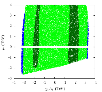
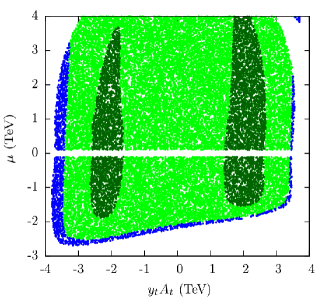
Figure 1: Scatter plots showing the regions with the DSB vacuum as the global minimum of the potential (green) and with an accompanying non-DSB CC minimum as the global minimum of the same (in blue) in the $y_{t}A_{t}$–$\mu$ plane. Plots in the left (right) panel are obtained from the SPheno-Vevacious (FeynHiggs-Mathematica) framework. The top (bottom) panel corresponds to $m_{\widetilde{Q}_{3}}=m_{\widetilde{U}_{3}}=m_{\widetilde{D}_{3}}=1\,\mathrm{TeV}\,(2$ TeV). Other fixed parameters are as follows: $M_{1}=M_{2}=750\,\mathrm{GeV}$ and $M_{3}=2$ TeV, $m_{A}=2$ TeV, $A_{b}=0$ and $\tan\beta=25$. The renormalization scale is set to $Q=\sqrt{m_{\widetilde{Q}_{3}}m_{\widetilde{U}_{3}}}$. Regions in dark-green are compatible with the observed SM-like Higgs boson (at $\sim 95\%$ C.L.) as reported by HiggsBounds and HiggsSignals.

The results of random scans over a relevant set of MSSM parameters showing the stability pattern of the DSB vacuum are presented in figure 1. Given that the top squark sector is expected to dominate in the radiative contributions to the potential, we choose the $y_{t}A_{t}$–$\mu$ plane for illustration. In each row, the left plot results from a Vevacious analysis of the spectra obtained from SARAH-generated SPheno where we indicate the regions that correspond to either a stable DSB vacuum (global minimum; in green) or the presence of an accompanying (non-DSB) global minimum (in blue). The corresponding right plots present the results of a similar analysis using the same set of MSSM input parameters but adopting the FeynHiggs-Mathematica framework. The top (bottom) panel corresponds to $m_{\widetilde{Q}_{3}}=m_{\widetilde{U}_{3}}=m_{\widetilde{D}_{3}}=1\,\mathrm{TeV}\,(2\,\mathrm{TeV})$. Ranges of various MSSM parameters that are scanned over and the fixed values for the others are indicated in the figure caption.

No CB minimum emerges, irrespective of whether it is deeper than the DSB vacuum or not. However, a deeper (panic) CC minimum, which is absent for the tree-level Higgs potential, might appear this time with its origin in the radiative correction to the said potential (Coleman-Weinberg type). Such deeper CC minima, however, appear only along the edges (in blue) of the displayed plane. A similar phenomenon associated with larger values of ‘$\mu$’, along with a decoupled gluino, has been observed in reference Bobrowski:2014dla which incorporates corrections to the potential from the third generation quarks and squarks only. Interestingly, as can be gleaned from figure 1, the inclusion of the full 1-loop correction to the potential (as is the case with both SPheno and FeynHiggs) results in such a panic CC minimum occurring even for relatively smaller values of ‘$\mu$’ and $A_{t}$. However, such regions of the MSSM parameter space appear to be not compatible with the observed mass of the SM-like Higgs boson (given by the dark-green bands). This (mostly) pre-empts the threat from an emerging deeper CC minimum destabilizing the DSB vacuum. The horizontal, blank stripes about $\mu=0$ indicate the ranges of unacceptable $\mu$-values dictated by experimental constraints, primarily from the chargino searches.

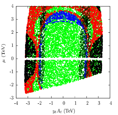
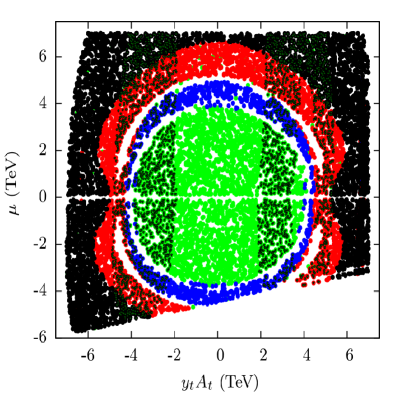
Figure 2: Stability status of the DSB vacuum in the presence of a deeper CC vacuum along with an unavoidable deeper CCB vacuum for the cases presented in the left panel (SPheno-Vevacious analyses) of figure 1. The left (right) plot corresponds to the top left (bottom left) plot of figure 1. The color code adopted is as follows: green stands for a stable DSB vacuum (global minimum), blue represents a metastable but cosmologically long-lived DSB vacuum, black indicates the presence of a DSB vacuum which is unstable under quantum tunneling at zero temperature while red corresponds to a DSB vacuum unstable against tunneling when the finite temperature corrections to the potential are included. The vertical bands in dark-green again delineate the regions compatible with the observed SM-like Higgs boson.

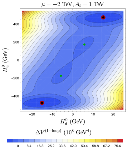
Figure 3: Potential ($\Delta V$) contours in the $H_{d}^{0}$–$H_{u}^{0}$ plane showing the (equivalent) locations of the DSB vacuum (blobs in green) and the accompanying global CC minimum (blobs in black-within-red). The magnitudes of $\Delta V$ can be estimated from the color-palette displayed underneath. The fixed MSSM parameters ‘$\mu$’ and $A_{t}$ are as indicated at the top of the plot. Other fixed parameters are as in figure 1 with $m_{\widetilde{Q}_{3}}=m_{\widetilde{U}_{3}}=m_{\widetilde{D}_{3}}=1$ TeV. See text for details.

In figure 2, we indicate the stability status of the DSB vacuum for the same set of data points and in the same parameter plane as for figure 1 but this time we allow for the colored sfermions assuming vevs. This is to check for likely appearances of deeper CCB vacua that could have already been triggered by the large values of $y_{t}A_{t}$ and/or ‘$\mu$’ that are necessary for a deeper CC vacuum to occur, as is seen in figure 1.

We indeed find an onset of a deeper CCB minimum just away from the central regions of these plots with much smaller values of $y_{t}A_{t}$ and ‘$\mu$’. This clearly indicates that long before a deeper CC minimum originating purely in the Higgs potential could pose a threat to the stability of the DSB vacuum, the scalar potential is inflicted with a dangerous CCB minimum. This may perhaps be easily comprehended by noting that both deeper CCB and CC minima are dominantly driven by the fermions and sfermions from the third generation; however, while the former could well be a tree-level effect, the latter have a genuine origin in the radiatively corrected potential.

In figure 3 we demonstrate the potential ($\Delta V$) contours in the $H_{d}^{0}$–$H_{u}^{0}$ plane, where $\Delta V$ is the relative depth with respect to the potential at the field origin. The location(s) of the DSB vacuum (deeper minimum) are indicated by the green (black-in-red) blobs. Such minima appearing in the first quadrant are the identical ones to those showing up in the third quadrant because of the underlying reflection symmetry of the potential.

Before concluding this section, one observation regarding occasional numerical (in)stability of the results obtained from Vevacious  may be noted. While working with two non-vanishing charged Higgs vevs, one encounters a CC minimum nearly degenerate with the DSB vacuum and situated very close to the latter in the field space. Under such a circumstance, due to limited floating point precision it uses, Vevacious  may find it difficult to decide the fate of the DSB vacuum correctly. However, this is a direct consequence of not exploiting the freedom to rotate one of the charged Higgs $vevs$ to start with. We further checked this via our Mathematica analysis using a much larger precision that it offers.

3 Spontaneous breakdown of charge: the $Z_{3}$-symmetric NMSSM case

It has recently been noted Muhlleitner:2016mzt in the context of a singlet-extended 2HDM (N2HDM) that the global minimum of the potential may not be a charge-conserving one at the tree-level, unlike in the 2HDM. This is attributed to the neutral singlet scalar field of such a scenario developing vev thereby mixing with the doublet Higgs states. Naturally, such an observation bears relevance to a scenario like the NMSSM where a similar effect can be investigated Maniatis:2006jd . In this section, we first take an analytical look into how the $Z_{3}$-symmetric NMSSM Higgs potential could develop a global CB minimum. A numerical, random scan of the NMSSM parameter space using Vevacious follows. This delineates the region of the parameter space offering a viable DSB vacuum.

3.1 Analysis of the tree-level Higgs potential: the NMSSM case

The tree-level Higgs potential of the $Z_{3}$-symmetric NMSSM is given by

$$V_{\mathrm{Higgs}} = \left|\lambda\left(H_{u}^{+}H_{d}^{-}-H_{u}^{0}H_{d}^{0}\right)+\kappa S^{2}\right|^{2}$$ (23)

$$+\left(m_{H_{u}}^{2}+\left|\lambda S\right|^{2}\right)\left(\left|H_{u}^{0}\right|^{2}+\left|H_{u}^{+}\right|^{2}\right)+\left(m_{H_{d}}^{2}+\left|\lambda S\right|^{2}\right)\left(\left|H_{d}^{0}\right|^{2}+\left|H_{d}^{-}\right|^{2}\right)$$

$$+\frac{g_{1}^{2}+g_{2}^{2}}{8}\left(\left|H_{u}^{0}\right|^{2}+\left|H_{u}^{+}\right|^{2}-\left|H_{d}^{0}\right|^{2}-\left|H_{d}^{-}\right|^{2}\right)^{2}+\frac{g_{2}^{2}}{2}\left|H_{u}^{+}H_{d}^{0*}+H_{u}^{0}H_{d}^{-*}\right|^{2}$$

$$+m_{S}^{2}|S|^{2}+\big{(}\lambda A_{\lambda}\left(H_{u}^{+}H_{d}^{-}-H_{u}^{0}H_{d}^{0}\right)S+\frac{1}{3}\kappa A_{\kappa}\,S^{3}+\mathrm{h.c.}\big{)}\>.$$

The set of (tree-level) tadpoles now includes the one for the singlet (neutral) scalar field ‘$S$’, over and above those for the doublet Higgs fields. All the tadpoles now involve $v_{{}_{S}}$, the vev for the field ‘$S$’. Similar to the MSSM case presented in section 2.1, with $T_{i}=\frac{\partial V_{\mathrm{Higgs}}}{\partial v_{i}}$, where ‘$i$’ stands for the field with respect to which a partial derivative is taken, these tadpoles are given by

$$T_{H_{u}^{0}}=0 = g^{2}v_{u}(v_{u}^{2}+v_{u^{+}}^{2}-v_{d}^{2}-v_{d^{-}}^{2})+2(m_{H_{u}}^{2}+\lambda^{2}v_{s}^{2})v_{u}+g_{2}^{2}v_{d^{-}}(v_{u}v_{d^{-}}+v_{u^{+}}v_{d})$$ (24a)

$$+\,2\lambda^{2}v_{d}(v_{u}v_{d}-v_{u^{+}}v_{d^{-}})-2\lambda v_{d}v_{s}(A_{\lambda}+\kappa v_{s})\>,$$

$$T_{H_{d}^{0}}=0 = -g^{2}v_{d}(v_{u}^{2}+v_{u^{+}}^{2}-v_{d}^{2}-v_{d^{-}}^{2})+2(m_{H_{d}}^{2}+\lambda^{2}v_{s}^{2})v_{d}+g_{2}^{2}v_{u^{+}}(v_{u}v_{d^{-}}+v_{u^{+}}v_{d})$$ (24b)

$$+\,2\lambda^{2}v_{u}(v_{u}v_{d}-v_{u^{+}}v_{d^{-}})-2\lambda v_{u}v_{s}(A_{\lambda}+\kappa v_{s})\>,$$

$$T_{H_{u}^{+}}=0 = g^{2}v_{u^{+}}(v_{u}^{2}+v_{u^{+}}^{2}-v_{d}^{2}-v_{d^{-}}^{2})+2(m_{H_{u}}^{2}+\lambda^{2}v_{s}^{2})v_{u^{+}}+g_{2}^{2}v_{d}(v_{u}v_{d^{-}}+v_{u^{+}}v_{d})$$ (24c)

$$-\,2\lambda^{2}v_{d^{-}}(v_{u}v_{d}-v_{u^{+}}v_{d^{-}})-2\lambda v_{d^{-}}v_{s}(A_{\lambda}+\kappa v_{s})\>,$$

$$T_{H_{d}^{-}}=0 = -g^{2}v_{d^{-}}(v_{u}^{2}+v_{u^{+}}^{2}-v_{d}^{2}-v_{d^{-}}^{2})+2(m_{H_{d}}^{2}+\lambda^{2}v_{s}^{2})v_{d^{-}}+g_{2}^{2}v_{u}(v_{u}v_{d^{-}}+v_{u^{+}}v_{d})$$ (24d)

$$-\,2\lambda^{2}v_{u^{+}}(v_{u}v_{d}-v_{u^{+}}v_{d^{-}})+2\lambda v_{u^{+}}v_{s}(A_{\lambda}+\kappa v_{s})\>,$$

$$T_{S}=0 = \lambda^{2}v_{s}(v_{u}^{2}+v_{u^{+}}^{2}+v_{d}^{2}+v_{d^{-}}^{2})+2v_{s}(m_{S}^{2}+\kappa A_{\kappa}v_{s}+2\kappa^{2}v_{s}^{2})$$ (24e)

$$-2\lambda(A_{\lambda}+\kappa v_{s})(v_{u}v_{d}-v_{u^{+}}v_{d^{-}})\>,$$

where $v_{u}$, $v_{d}$, $v_{u^{+}}$ and $v_{d^{-}}$ are as defined in section 2.1 and $v_{{}_{S}}={\mu_{\mathrm{eff}}\over\lambda}$. As before, we solve for the squared soft masses (tree-level) for the neutral Higgs states (including the singlet scalar) at the DSB vacuum. These are given by

$$m_{H_{d}}^{2} = -\mu_{\mathrm{eff}}^{2}-\lambda^{2}v_{u}^{2}-\frac{g_{1}^{2}+g_{2}^{2}}{4}(v_{d}^{2}-v_{u}^{2})+\mu_{\mathrm{eff}}(A_{\lambda}+\kappa v_{{}_{S}})\tan\beta\>,$$ (25a)

$$m_{H_{u}}^{2} = -\mu_{\mathrm{eff}}^{2}-\lambda^{2}v_{d}^{2}-\frac{g_{1}^{2}+g_{2}^{2}}{4}(v_{u}^{2}-v_{d}^{2})+\mu_{\mathrm{eff}}(A_{\lambda}+\kappa v_{{}_{S}})\cot\beta\;,$$ (25b)

$$m_{S}^{2} = -\kappa A_{\kappa}v_{{}_{S}}-2\kappa^{2}v_{{}_{S}}^{2}-\lambda^{2}(v_{d}^{2}+v_{u}^{2})+2\lambda\kappa v_{u}v_{d}+\lambda\frac{v_{u}v_{d}}{v_{{}_{S}}}A_{\lambda}\;.$$ (25c)

By substituting the squared soft masses from equation 25 into the potential of equation 23, one finds the expression for the tree-level depth of the DSB vacuum as

$$V^{{}^{\mathrm{DSB}}}_{\mathrm{Higgs}}|_{{}_{\mathrm{tree}}} = -\kappa^{2}v_{{}_{S}}^{4}-\frac{1}{3}\kappa A_{\kappa}v_{{}_{S}}^{3}-\lambda^{2}v_{{}_{S}}^{2}(v_{d}^{2}+v_{u}^{2})-\lambda v_{{}_{S}}v_{d}v_{u}(A_{\lambda}+2\lambda v_{{}_{S}})$$ (26)

$$-\frac{g_{1}^{2}+g_{2}^{2}}{8}(v_{d}^{2}-v_{u}^{2})^{2}-\lambda^{2}v_{d}^{2}v_{u}^{2}\;.$$

As earlier, to find possible deeper minima, we look for some flat directions in the field space. The $D$-flat directions are given by the same set of equations as in equation 16. In addition, there is now an $F$-flat direction given by

$$\lambda(v_{u^{+}}v_{d^{-}}-v_{u}v_{d})+\kappa v_{{}_{S}}^{2}=0\;.$$ (27)

A first study exploiting this flat direction has recently been discussed in reference Krauss:2017nlh . Along this $F$-flat direction the tadpole equation for the singlet scalar field ‘$S$’ has the following two independent solutions

$$v_{{}_{S}} = 0\;,$$ (28a)

$$v_{u}^{2}+v_{d}^{2}+v_{u^{+}}^{2}+v_{d^{-}}^{2} = {-2\over\lambda^{2}}\left[m_{S}^{2}+\kappa v_{{}_{S}}\left(A_{\kappa}-A_{\lambda}+\kappa v_{{}_{S}}\right)\right]\>.$$ (28b)

Solution 28a, when plugged in into the tadpole conditions $T_{H_{d}^{0}}=0$ and $T_{H_{d}^{-}}=0$, gives $v_{d}=v_{d^{-}}=0$ as a trivial possibility. However, such a solution does not yield a CB minimum since the only non-vanishing charged Higgs vev $v_{u^{+}}$ can now be rotated away in the presence of a non-vanishing $v_{u}$. Thus, by feeding $v_{d}=v_{d^{-}}=0$  to the tadpole conditions $T_{H_{u}^{0}}=0$ and $T_{H_{u}^{+}}=0$, we find, at the CC minimum,

$$v_{u}^{2}+v_{u^{+}}^{2}=-2\frac{m_{H_{u}}^{2}}{g^{2}}\>,$$ (29)

with its depth given by

$$V_{\mathrm{Higgs}(u)}^{\mathrm{CC}}={-m_{H_{u}}^{4}\over g^{2}}\>.$$ (30)

Clearly, the value of the potential at this CC minimum is negative. Also, for larger values of $m_{{}_{H_{u}}}^{2}$, the potential could turn out to be deeper than the DSB vacuum at the tree-level itself, a possibility that is in clear contrast to the MSSM case. This is intimately connected to the magnitude of $\mu_{\mathrm{eff}}$ as can be seen from equation 25b. Note that we would have arrived at the corresponding set of relations involving $v_{d}$, $v_{d^{-}}$ and $m_{H_{d}}$ had we, instead, chosen to plug in the first solution ($v_{{}_{S}}=0$) into the tadpole conditions $T_{H_{u}^{0}}=0$ and $T_{H_{u}^{+}}=0$, i.e.,

$$v_{d}^{2}+v_{d^{-}}^{2}=-2\frac{m_{H_{d}}^{2}}{g^{2}}\>,$$ (31)

with its depth given by

$$V_{\mathrm{Higgs}(d)}^{\mathrm{CC}}={-m_{H_{d}}^{4}\over g^{2}}\>.$$ (32)

A deeper CC minimum could also appear along a direction $v_{s}\neq 0$, with all other vevs set to zero, since such a configuration is always a solution to the tadpoles. The depth of such a minimum is given by

$$V_{\mathrm{Higgs}}^{\mathrm{CC}}\Big{\rvert}_{v_{{}_{S}}\neq 0}=v_{s}^{2}m_{S}^{2}+\kappa^{2}v_{s}^{4}+\frac{2}{3}\kappa A_{\kappa}v_{s}^{3}\;.$$ (33)

This can give rise to two non-zero minima with

$$v_{s}=\Bigg{\{}\frac{-(A_{\kappa}+\sqrt{A_{\kappa}^{2}-8m_{S}^{2}})}{4\kappa},\;\frac{-(A_{\kappa}-\sqrt{A_{\kappa}^{2}-8m_{S}^{2}})}{4\kappa}\Bigg{\}}\;.$$ (34)

The corresponding depths can be shown to possess non-negative potential values if one of the following conditions are satisfied Beuria:2016cdk

$$A_{\kappa}<-3\sqrt{A_{\kappa}^{2}-8m_{S}^{2}}\quad\mathrm{or}\quad A_{\kappa}>3\sqrt{A_{\kappa}^{2}-8m_{S}^{2}}\;.$$ (35)

As we will see later, in the presence of such a CC minimum with non-negative potential (and hence not so deep), a CB minimum could eventually turn out to be the global minimum (the effective panic vacuum) of the potential.

We now turn to a possible CB minimum. Its presence is conveniently studied in the rotated basis (introduced in equation 14) with $v_{u^{+}}^{\prime}=v_{d}^{\prime}=0$  or  $v_{d^{-}}^{\prime}=v_{u}^{\prime}=0$. Since the $F$-flat direction mentioned in equation 27 yields $v_{s}=0$ as a solution, this is consistent with the direction $v_{u^{+}}^{\prime}v_{d^{-}}^{\prime}=v_{u}^{\prime}v_{d}^{\prime}$. Choosing $v_{d^{-}}^{\prime}=v_{u}^{\prime}=0$, we obtain the following solutions for $v_{d}^{\prime}$ and $v_{u^{+}}^{\prime}$ from the tadpole conditions in equation 24:

$$|v_{d}^{\prime}|=\frac{\sqrt{-(g_{1}^{2}+g_{2}^{2})m_{{}_{H_{d}}}^{2}+(g_{2}^{2}-g_{1}^{2})m_{{}_{H_{u}}}^{2}}}{g_{1}g_{2}}\;,$$ (36a)

$$|v_{u^{+}}^{\prime}|=\frac{\sqrt{-(g_{1}^{2}+g_{2}^{2})m_{{}_{H_{u}}}^{2}+(g_{2}^{2}-g_{1}^{2})m_{{}_{H_{d}}}^{2}}}{g_{1}g_{2}}\;.$$ (36b)

The depth of the potential is given by

$$V_{\mathrm{Higgs}}^{\mathrm{CB}}=-\left[\frac{g_{1}^{2}(m_{H_{d}}^{2}+m_{H_{u}}^{2})^{2}+g_{2}^{2}(m_{H_{d}}^{2}-m_{H_{u}}^{2})^{2}}{2g_{1}^{2}g_{2}^{2}}\right]\;,$$ (37)

which is clearly always negative. For the vevs in equation 36 to be real, one requires the following sets of inequalities to hold simultaneously:

$$\frac{g_{1}^{2}+g_{2}^{2}}{g_{2}^{2}-g_{1}^{2}}m_{{}_{H_{u}}}^{2} < m_{{}_{H_{d}}}^{2}<\frac{g_{2}^{2}-g_{1}^{2}}{g_{1}^{2}+g_{2}^{2}}m_{{}_{H_{u}}}^{2}\;,$$ (38a)

$$m_{{}_{H_{u}}}^{2} < 0,\quad m_{{}_{H_{d}}}^{2}<0\;.$$ (38b)

For typical values of $g_{1}$ and $g_{2}$, the inequality in equation 38a approximately reduces to

$$2m_{{}_{H_{u}}}^{2}<m_{{}_{H_{d}}}^{2}<0.5m_{{}_{H_{u}}}^{2}\;.$$ (39)

At this point, using soft mass-squared terms mentioned in equations 25a and 25b, for $\tan\beta>\sqrt{2}$ and $\mu_{\mathrm{eff}}>0$, we obtain the following approximate inequality:

$$v_{0}^{2}\frac{\tan\beta}{\mu_{\mathrm{eff}}(1+\tan^{2}\beta)}\left(\lambda^{2}-0.4\frac{\tan^{2}\beta-1}{\tan^{2}\beta-2}\right)-\left(\frac{\tan\beta}{\tan^{2}\beta-2}+\frac{\kappa}{\lambda}\right)\mu_{\mathrm{eff}}\;\;< A_{\lambda}$$ (40)

$$<\;v_{0}^{2}\frac{\tan\beta}{\mu_{\mathrm{eff}}(1+\tan^{2}\beta)}\left(\lambda^{2}-0.4\frac{\tan^{2}\beta-1}{2\tan^{2}\beta-1}\right)+\left(\frac{\tan\beta}{2\tan^{2}\beta-1}-\frac{\kappa}{\lambda}\right)\mu_{\mathrm{eff}}\;,$$

and for $1<\tan\beta<\sqrt{2}$ and $\mu_{\mathrm{eff}}>0$, similarly, we find

$$A_{\lambda}<v_{0}^{2}\frac{\tan\beta}{\mu_{\mathrm{eff}}(1+\tan^{2}\beta)}\left(\lambda^{2}-0.4\frac{\tan^{2}\beta-1}{2\tan^{2}\beta-1}\right)+\left(\frac{\tan\beta}{2\tan^{2}\beta-1}-\frac{\kappa}{\lambda}\right)\mu_{\mathrm{eff}}\;.$$ (41)

The expressions for the lower and/or the upper limits of the inequalities in equations 40 and 41 swap their positions for $\mu_{\mathrm{eff}}<0$. From these two equations, it is clear that appearance of a CB minimum explicitly depends on the set of four parameters, i.e., {$A_{\lambda}$, $\tan\beta$, $\kappa\over\lambda$, $\mu_{\mathrm{eff}}$}. In addition, other parameters such as $A_{\kappa}$ could work in tandem with a chosen set of these four parameters to yield a consistent, non-tachyonic spectrum for the DSB vacuum and in rendering the accompanying CB minimum global. It may also be noted that a recent work Krauss:2017nlh has addressed similar issues, guided by $\tan\beta\approx 1$. We have checked that the inequality in 41, in the limit $\tan\beta\to 1$, leads to observations that agree with those of reference Krauss:2017nlh . On the other hand, the inequality in 40 that refers to $\tan\beta>\sqrt{2}$, explores further regions in the NMSSM parameter space where a deeper CB minimum could pose a genuine threat to the stability of the DSB vacuum.

It is thus clear from the above discussion that both CC and CB minima that are deeper than the DSB vacuum could appear simultaneously for a tree-level NMSSM Higgs potential. We have further checked that the inequalities pertaining to the CB minima (expressions 40 and 41) imply those to be deeper than a CC minimum arising along the direction $v_{{}_{S}}=0$ (always having a negative potential value; see equations 30 and 32). Note that the value of the potential at a CB minimum is always negative (see equation 37). In the presence of a CB minimum deeper than the DSB vacuum, the “globality” of the former is conservatively ensured if a CC minimum along $v_{{}_{S}}\neq 0$ (equation 33, singlet-only direction) has a positive potential. The latter is achieved if $A_{\kappa}$ can be constrained as in equation 35. The requirement of non-tachyonic Higgs states further restricts the allowed ranges of $A_{\lambda}$ and $A_{\kappa}$.

In the present analysis, we deal with a somewhat broader region of the NMSSM parameter space (when compared to reference Krauss:2017nlh ) that yields deeper CB minima. This is facilitated by a relatively large radiative correction to the potential. Thus, guided by equation 40, we expect to find regions with a global CB minimum even for relatively low values of $|\mu_{\mathrm{eff}}|$ when ${\kappa\over\lambda}>1$. In that case, $|A_{\lambda}|$ can be larger than $|\mu_{\mathrm{eff}}|$. Furthermore, we also take into account the effect of thermal correction to the potential.

3.2 Scanning of the NMSSM parameter space

In this section, we present and discuss the results of our scan over the NMSSM parameter space using the package Vevacious. This would shed light on regions of the said parameter space with diverse kind of stability properties of the DSB vacuum, without and with the inclusion of thermal contributions to the potential. As has been noted in section 2.2, we have tweaked Vevacious so as to find the most relevant ‘panic’ vacuum. It may be mentioned here that we have not seen any significant impact of such a modification in the MSSM case. However, reference Krauss:2017nlh has recently pointed out that the issue becomes important in the NMSSM case, an observation on which we concur.

The analysis presented in section 3.1 prompts us to divide the scan into two categories: (i) one which is suited for exploring a deeper CB minimum guided by equations 40 and 41 and for which we take fixed values of $\mu_{\mathrm{eff}}$ and $\kappa$ while $A_{\lambda}$ and $A_{\kappa}$ are varied and (ii) the other which is tailored to find (mostly) a deeper CC minimum, guided by equation 35, for which $A_{\kappa}$ is kept fixed while $A_{\lambda}$, $\mu_{\mathrm{eff}}$ and $\kappa$ are varied. Note that, from equation 23, $\kappa$ and $A_{\kappa}$ govern the pure singlet contribution to the NMSSM Higgs potential. Varying one or the other of these two parameters at a time would shed light on how and to what extent the singlet sector carves out a CC or CB minimum, possibly deeper than the DSB vacuum. For both cases, we hold $\lambda$ and $\tan\beta$ fixed at an optimal, common set of values. We discuss these cases in the next two subsections. All through, we keep track of the regions compatible with the observed SM-like Higgs boson by using the packages HiggsSignals and HiggsBounds.

3.2.1   Hunt for deeper charge-breaking minima: case with fixed $\mu_{\mathrm{eff}}$ and $\kappa$

In this subsection, we present the results of a random scan over a large region in the $A_{\lambda}$–$A_{\kappa}$ plane keeping $\mu_{\mathrm{eff}}$, $\kappa$ and some other parameters fixed at suitable values. A closer look at equation 37, in conjunction with equations 25a and 25b, would help us decide on the strategy for scanning the NMSSM parameter space. As we have seen in section 3.1, one of the dangerous directions (an $F$-flat direction) along which a CB minimum could appear is $v_{{}_{S}}=0$. Its appearance, however, is facilitated by ensuring, to start with, a shallower potential at the DSB vacuum. From the inequalities in equations 40 and 41 that are required to be satisfied for CB minima to occur, we find that somewhat large values of $\lambda$ and $\mu_{\mathrm{eff}}$ along with low values of $\tan\beta$ help. Hence we fix $\lambda$ to a moderately large value of 0.7 and take $\tan\beta=2$. In addition, we take a somewhat large value of $\kappa=1$ which, as discussed at the end of the last subsection, help ensure ${\kappa\over\lambda}>1$ thus enabling exploration of a deeper CB minimum for somewhat larger values $|A_{\lambda}|$. To demonstrate the latter, we choose two representative values of $\mu_{\mathrm{eff}}$. Furthermore, two sets of values of soft parameters ($m_{\widetilde{Q}_{3}}=m_{\widetilde{U}_{3}}$ and $A_{t}$) in the top squark sector (yielding small/large masses/mixings) are chosen for the purpose. These amount to a varied extent of radiative correction to the potential. Such choices are expected to alter the spans of the parameter plane inflicted with panic vacua of both CC and CB types.

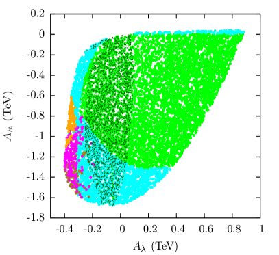
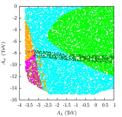
Figure 4: Scatter plots obtained from a random scan over $A_{\lambda}$ and $A_{\kappa}$ and showing the stability pattern of the DSB vacuum in the $A_{\lambda}$–$A_{\kappa}$ plane for $\mu_{\mathrm{eff}}=300$ GeV (3 TeV) in the left (right) plot. The color code is summarized in table 1. Other important fixed parameters are $m_{\widetilde{Q}_{3}}=m_{\widetilde{U}_{3}}=750$ GeV, $A_{t}=0$, $\lambda=0.7$ and $\kappa=1$.

In figure 4, we present the region in the $A_{\lambda}$–$A_{\kappa}$ parameter plane which possesses a DSB vacuum and may be accompanied by a CC and/or a CB minimum which are/is deeper than the former. The color code described in table 1 indicates only the presence and nature (CC or CB) of such ‘panic’ minima and not yet tells anything about whether such panic minima are dangerous for the stability of the DSB vacuum. The figure represents the case with low stop masses ($\approx 750$ GeV) and with $\mu_{\mathrm{eff}}=300\,\mathrm{GeV}\,(3\,\mathrm{TeV})$ for the left (right) plot. It may be noted that the ranges of $A_{\lambda}$ and $A_{\kappa}$ are much larger for the plot on the right with $\mu_{\mathrm{eff}}=3$ TeV when compared to the left plot with $\mu_{\mathrm{eff}}=300$ GeV. This is since by increasing $\mu_{\mathrm{eff}}$ and hence $\kappa v_{S}$, one could accommodate large negative values of $A_{\kappa}$ and $A_{\lambda}$ consistent with a non-tachyonic Higgs spectrum. We now find a deeper CB minimum appearing for such large negative values of $A_{\lambda}$ and $A_{\kappa}$. From equation 40 and 41 we find that $A_{\lambda}$ is governed by $-{\kappa\over\lambda}\mu_{\mathrm{eff}}$ for small values of $\tan\beta$. For this figure, ${\kappa\over\lambda}>1$ and hence the region of CB minima appears around $A_{\lambda}<-\mu_{\mathrm{eff}}$. Accordingly, this fixes the range of $A_{\kappa}$ so that tachyonic states are avoided, as pointed out above. Note that a flip of sign on $\mu_{\mathrm{eff}}$ results in altered signs on both $A_{\lambda}$ and $A_{\kappa}$ to find such regions with a deeper/global CB minimum.

Color	Green	Cyan	Orange	Brown	Magenta	Dark-green
Deeper vacua	DSB only	Deeper CC	Deeper CC	Deeper CB	Deeper CB	—
present		No deeper CB	Deeper CB	No Deeper CC	Deeper CC
Observation	DSB Global	CC Global	CC Global	CB Global	CB Global	Allowed by
						Higgs data

Table 1: Color code used in figures 4 and 5 to indicate the presence of minima deeper than the DSB vacuum, their nature (CC or CB) and the one that is the global minimum of the potential.

It would be now interesting to study the impact of a large radiative correction to the potential. Such large corrections are easily achieved with larger values of masses and mixings in the top squark sector. We thus fix $m_{\widetilde{Q}_{3}}=m_{\widetilde{U}_{3}}=3$ TeV and $A_{t}=1$ TeV, keeping other fixed parameters the same as in figure 4. Figure 5 illustrates the case. The left plot (with $\mu_{\mathrm{eff}}=300$ GeV) of figure 5 hints a shrinking of the region featuring a deeper CB vacuum (in orange, red and magenta) when compared to the corresponding one of figure 4. However, radiative effects are amplified for larger values of $\mu_{\mathrm{eff}}$ ($\sim m_{\widetilde{Q}_{3}},\;m_{\widetilde{U}_{3}}$), as can be seen by comparing the right plots of these two figures.

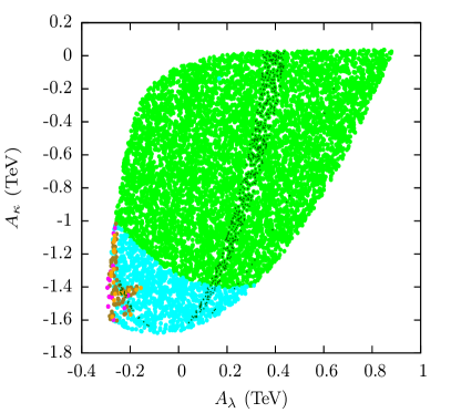
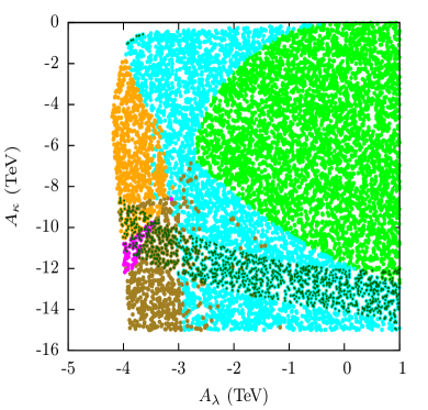
Figure 5: Same as in figure 4 but for $m_{\widetilde{Q}_{3}}=m_{\widetilde{U}_{3}}=3$ TeV, $A_{t}=1$ TeV.

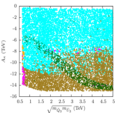
Figure 6: Same as in figure 4 but in the $\sqrt{m_{\widetilde{Q}_{3}}m_{\widetilde{U}_{3}}}\,$–$\,A_{\kappa}$ plane. The fixed parameters are also as in figures 4 except for $\mu_{\mathrm{eff}}=-A_{\lambda}=3$ TeV and $A_{t}=m_{\widetilde{Q}_{3}}=m_{\widetilde{U}_{3}}$.

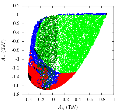
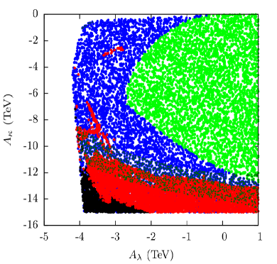
Figure 7: Scatter plots showing the stability status of the DSB vacuum in the $A_{\lambda}$–$A_{\kappa}$ plane in the presence of a deeper CB minimum. Color code in use are as adopted for figure 2. The left (right) plot corresponds to the same set of data points as used in the left plot of figure 4 (right plot of figure 5).

It may be summarized from figures 4 and 5 that a CB vacuum could turn out to be the global minimum of the potential over an appreciable region of parameter space for relatively large values of $A_{\lambda}$, $A_{\kappa}$, $\mu_{\mathrm{eff}}$ and parameters in the top squark sector and for $\tan\beta$ on the smaller side. Under the circumstances, the global CB minimum could either be the lone deeper minimum (in “red”) or can be accompanied by a CC minimum which is shallower than it, but still deeper than the DSB vacuum (in “magenta”). Note that with increased values of soft parameters in the top squark sector a global CB minimum becomes increasingly compatible to observed Higgs boson properties. Thus, a priori, such CB minima should be considered as dangerous for the stability of the DSB vacuum. This warrants dedicated studies of vacuum configurations of the potential by including vevs for the charged Higgs states.

The extent of the impact of radiative correction to the potential is further investigated in the plane $\sqrt{m_{\widetilde{Q}_{3}}m_{\widetilde{U}_{3}}}$ – $A_{\kappa}$ as illustrated in figure 6. Here, we consider $\mu_{\mathrm{eff}}=3$ TeV and $A_{\lambda}=-3$ TeV. Clearly, the larger the (soft) masses for the top squarks, the larger is the region in the parameter plane that possesses a global CB minimum (without an accompanying deeper CC minimum (in red)) which remains to be compatible with the observed Higgs data. Absence of a “green” region in this plot only indicates that the DSB vacuum never becomes the global minimum of the potential for such a set of NMSSM parameters and hence lives dangerously.

Finally, the fate of the DSB vacua in the presence of a deeper minimum (CC or CB) is determined by calculating how fast could the former tunnel to the latter. A viable DSB vacuum is either the global minimum of the potential or its lifetime is comparable (or larger) than the age of the Universe. In figure 7 we profile such regions in the $A_{\lambda}$-$A_{\kappa}$ plane on the basis of stability (viability) of the DSB vacuum against tunneling to a deeper minimum. For a straightforward comparison, we choose the left (right) plot of this figure to correspond to the left plot of figure 4 (right plot of figure 5). We observe that significant portions of the parameter plane characterized primarily by large $A_{\kappa}$ could get ruled out due to fast tunneling of the DSB vacuum which is triggered by thermal effects. Such a finding is in agreement with the observations made in reference Beuria:2016cdk but now is generalized to the case where CB minimum deeper than the DSB vacuum is a possibility.

It may be noted here that unlike in the case of the MSSM, a deeper CB minimum could arise without a conventional CCB minimum being triggered. CCB directions, that otherwise could be dangerous, can be avoided in the presence of singlet $vevs$ since the latter might contribute positively to the potential Ellwanger:1999bv ; Kanehata:2011ei . In fact, our Vevacious scan mostly indicates the region of parameter space for figure 6 to be CCB safe. We verify this by allowing for $vevs$ for the stops in our Vevacious analysis. For a rough understanding of the phenomenon, we impose the relevant (tree level) criteria mentioned in Ellwanger:1999bv ; Kanehata:2011ei on our Vevacious outputs and find the above mentioned region is mostly CCB safe.

3.2.2   Hunt for deeper charge-conserving minima: case with a fixed $A_{\kappa}$

In this subsection, we present the results of a random scan in the $A_{\lambda}$–$\mu_{\mathrm{eff}}$ plane keeping $A_{\kappa}$ fixed but allowing $\mu_{\mathrm{eff}}$ and $\kappa$ to vary over moderate ranges, as would suffice for the purpose. We take $A_{\kappa}=-1.5$ TeV and set $m_{\widetilde{Q}_{3}}=m_{\widetilde{U}_{3}}=1$ TeV with $A_{t}=0$. We stick to the choice of $\lambda=0.7$ and $\tan\beta=2$ made in the previous section. The scan is already subjected to the scrutiny of HiggsSignals and HiggsBounds. Hence the results presented would be straightaway compatible with the observed SM-like Higgs boson.

In the left plot of figure 8 we illustrate the stability status of the DSB vacuum in the $A_{\lambda}$–$\mu_{\mathrm{eff}}$ plane. The ranges of the parameters that are made to vary are indicated in the figure caption.

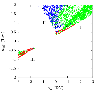
Figure 8: Scatter plots showing stability status of the DSB vacuum in the $A_{\lambda}$–$\mu_{\mathrm{eff}}$ plane (left) and in the $v_{c}$–$v_{n}$ plane (right). Color code employed is as for figure 7. Ranges of various NMSSM parameters that are randomly scanned over are $|\mu_{\mathrm{eff}}|<2$ TeV, $|\kappa|<0.75$ and $|A_{\lambda}|<3$ TeV while the fixed NMSSM parameters are $\lambda=0.7$, $\tan\beta=2$, $m_{\widetilde{Q}_{3}}=m_{\widetilde{U}_{3}}=1$ TeV, $A_{t}=0$ and $A_{\kappa}=-1.5$ TeV. All data points pass the constraints coming from HiggsSignals and HiggsBounds.

Regions I and II correspond to $\kappa>0$ whereas region III has $\kappa<0$. Region I is found to have a stable DSB vacuum (in green) for larger values of $A_{\lambda}$. This can be understood by looking at the $A_{\lambda}$-dependent term in equation 23. Furthermore, the same term predicts that the situation could change dramatically if $A_{\lambda}$ and $\mu_{\mathrm{eff}}$ carry a relative sign since the DSB vacuum could then become shallower relative to other non-DSB minima of the potential that might be present. Region II represents such a situation. However, the DSB vacuum is found to be mostly long-lived (in blue) over this region. We observe that metastable DSB vacua could also appear for values of $|\mu_{\mathrm{eff}}|<1$ TeV which are eventually found to be thermally unstable (in red) thanks to a moderately large value of $A_{\kappa}$ Beuria:2016cdk that we use. It may be noted that for such regions, $\mu_{\mathrm{eff}}$ and $A_{\lambda}$ carry the same sign. From what we learn from the previous section, these are unlikely to be the CB minima and are merely the deeper (and dangerous) CC minima. On the other hand, the metastable (blue) points in region II could have either kind of minima. Region III has got negative $\kappa$ and hence requires both $A_{\lambda}$ and $\mu_{\mathrm{eff}}$ to be negative as well to ensure a non-tachyonic Higgs spectrum.

A corroborative insight into nature of these dangerous vacua can be drawn from the right plot of figure 8. This is a scatter plot projecting the data points of the left plot in the $v_{c}$–$v_{n}$ plane, where $v_{c}=\sqrt{v_{u^{+}}^{2}+v_{d^{-}}^{2}}$ and $v_{n}=\sqrt{v_{u}^{2}+v_{d}^{2}}$. As has been discussed in section 2.1, CC vacua could only appear along the $D$-flat direction mentioned in equation 16a. Deeper vacua that mostly conserve charge form circular patterns which can be understood by looking at equations 29 and 31. This is further corroborated by a vanishing photon mass arising with such a system of vevs. A small arc of radius ($v_{c}^{2}+v_{n}^{2}\approx 174$ GeV) in green, close to the origin, represents an equivalent set of DSB vacua connected via $SU(2)$ transformations. Just beyond this, a narrow belt in red represents the vev combinations leading to deeper minima which make the DSB vacuum for each case thermally unstable. Further away from the origin, a metastable DSB vacuum survives tunneling and becomes long-lived (in blue).

4 Conclusions

In this work, we have studied the possibilities and the implications of a spontaneous breakdown of charge, triggered by the charged Higgs states acquiring vevs, in popular SUSY scenarios like the MSSM and the NMSSM.

It has been known for some time that in a generic 2HDM, in the presence of a charge-conserving minimum, the tree-level Higgs potential cannot have a deeper minimum where charge breaks spontaneously. The MSSM being a SUSY extension of such a scenario is not an exception. In fact, rigorous studies from the past had already established that the tree-level MSSM potential cannot even have a second minimum, either of CC or CB type, once it offers a DSB vacuum. In the present work, we show that when quantum corrections are included in the MSSM potential, a deeper CC minimum could arise along the $D$-flat directions together with the DSB vacuum. A Vevacious-based thorough scan of the MSSM parameter space reveals that such a deeper CC minimum is always accompanied by a conventional CCB minimum. Furthermore, regions of the parameter space where such a CC minimum appears are hardly ever compatible with the observed SM-like Higgs boson. Hence, on both counts, such a deeper CC minimum cannot emerge as an exclusive threat to the stability of the DSB vacuum. On the other hand, an accompanying deeper CB minimum never shows up. These findings are further corroborated by our alternate analysis using the FeynHiggs-Mathematica framework. The role of thermal correction to the potential is also discussed.

The situation is characteristically different in the NMSSM thanks to the presence of a neutral, SM-singlet scalar field. Here, a deeper CB minimum along with a CC one of a similar nature could already occur with the tree-level Higgs potential. Thus, checking for the stability of the DSB vacuum becomes a rather involved task, more so when radiative corrections to the potential are included. The issue has also been recently studied in reference Krauss:2017nlh . We broadly agree with the inferences of that work. However, we further note that there may be regions in the NMSSM parameter space, though a little remote to the ones studied in reference Krauss:2017nlh , where a deeper CB minimum could arise. Unlike in the case of the MSSM, there may not be any accompanying deeper CCB minimum. Hence such a CB minimum could pose a genuine threat to the stability of the DSB vacuum and hence should not get overlooked.

We also demonstrate that, in the process, thermal corrections to the potential are, in general, crucial and ignoring them could lead to grossly incorrect information on the stability of the DSB vacuum.

- (1) P. M. Ferreira, R. Santos and A. Barroso, “Stability of the tree-level vacuum in two Higgs doublet models against charge or CP spontaneous violation,” Phys. Lett. B 603 (2004) 219 Erratum: [Phys. Lett. B 629 (2005) 114] [hep-ph/0406231].
- (2) A. Barroso, P. M. Ferreira and R. Santos, “Charge and CP symmetry breaking in two Higgs doublet models,” Phys. Lett. B 632 (2006) 684 [hep-ph/0507224].
- (3) M. Maniatis, A. von Manteuffel, O. Nachtmann and F. Nagel, “Stability and symmetry breaking in the general two-Higgs-doublet model,” Eur. Phys. J. C 48 (2006) 805 [hep-ph/0605184].
- (4) A. Barroso, P. M. Ferreira, I. P. Ivanov and R. Santos, “Metastability bounds on the two Higgs doublet model,” JHEP 1306 (2013) 045 [arXiv:1303.5098 [hep-ph]].
- (5) A. Barroso, P. M. Ferreira, R. Santos and J. P. Silva, “Stability of the normal vacuum in multi-Higgs-doublet models,” Phys. Rev. D 74 (2006) 085016 [hep-ph/0608282].
- (6) F. Staub, “Reopen parameter regions in Two-Higgs Doublet Models,” arXiv:1705.03677 [hep-ph].
- (7) L. Alvarez-Gaume, J. Polchinski and M. B. Wise, “Minimal Low-Energy Supergravity,” Nucl. Phys. B 221 (1983) 495.
- (8) J. F. Gunion, H. E. Haber and M. Sher, “Charge / Color Breaking Minima and a-Parameter Bounds in Supersymmetric Models,” Nucl. Phys. B 306 (1988) 1.
- (9) J. A. Casas, A. Lleyda and C. Munoz, “Strong constraints on the parameter space of the MSSM from charge and color breaking minima,” Nucl. Phys. B 471 (1996) 3 [hep-ph/9507294].
- (10) A. Strumia, “Charge and color breaking minima and constraints on the MSSM parameters,” Nucl. Phys. B 482 (1996) 24 [hep-ph/9604417].
- (11) H. Baer, M. Brhlik and D. Castano, “Constraints on the minimal supergravity model from nonstandard vacua,” Phys. Rev. D 54 (1996) 6944 [hep-ph/9607465].
- (12) S. A. Abel and C. A. Savoy, “Charge and color breaking constraints in the MSSM with nonuniversal SUSY breaking,” Phys. Lett. B 444 (1998) 119 [hep-ph/9809498].
- (13) S. Abel and T. Falk, “Charge and color breaking in the constrained MSSM,” Phys. Lett. B 444 (1998) 427 [hep-ph/9810297].
- (14) D. Chowdhury, R. M. Godbole, K. A. Mohan and S. K. Vempati, “Charge and Color Breaking Constraints in MSSM after the Higgs Discovery at LHC,” JHEP 1402 (2014) 110 [arXiv:1310.1932 [hep-ph]].
- (15) N. Blinov and D. E. Morrissey, “Vacuum Stability and the MSSM Higgs Mass,” JHEP 1403 (2014) 106 [arXiv:1310.4174 [hep-ph]].
- (16) W. G. Hollik, “Charge and color breaking constraints in the Minimal Supersymmetric Standard Model associated with the bottom Yukawa coupling,” Phys. Lett. B 752 (2016) 7 [arXiv:1508.07201 [hep-ph]].
- (17) W. G. Hollik, “A new view on vacuum stability in the MSSM,” JHEP 1608 (2016) 126 [arXiv:1606.08356 [hep-ph]].
- (18) J. E. Camargo-Molina, B. Garbrecht, B. O’Leary, W. Porod and F. Staub, “Constraining the Natural MSSM through tunneling to color-breaking vacua at zero and non-zero temperature,” Phys. Lett. B 737 (2014) 156 [arXiv:1405.7376 [hep-ph]].
- (19) U. Chattopadhyay and A. Dey, “Exploring MSSM for Charge and Color Breaking and Other Constraints in the Context of Higgs@125 GeV,” JHEP 1411 (2014) 161 [arXiv:1409.0611 [hep-ph]].
- (20) U. Ellwanger, M. Rausch de Traubenberg and C. A. Savoy, “Phenomenology of supersymmetric models with a singlet,” Nucl. Phys. B 492 (1997) 21 [hep-ph/9611251].
- (21) U. Ellwanger and C. Hugonie, “Constraints from charge and color breaking minima in the (M+1)SSM,” Phys. Lett. B 457 (1999) 299 [hep-ph/9902401].
- (22) Y. Kanehata, T. Kobayashi, Y. Konishi, O. Seto and T. Shimomura, “Constraints from Unrealistic Vacua in the Next-to-Minimal Supersymmetric Standard Model,” Prog. Theor. Phys. 126 (2011) 1051 [arXiv:1103.5109 [hep-ph]].
- (23) T. Kobayashi, T. Shimomura and T. Takahashi, “Constraining the Higgs sector from False Vacua in the Next-to-Minimal Supersymmetric Standard Model,” Phys. Rev. D 86 (2012) 015029 [arXiv:1203.4328 [hep-ph]].
- (24) J. Beuria, U. Chattopadhyay, A. Datta and A. Dey, “Exploring viable vacua of the Z3-symmetric NMSSM,” JHEP 1704 (2017) 024 [arXiv:1612.06803 [hep-ph]].
- (25) U. Ellwanger, C. Hugonie and A. M. Teixeira, “The Next-to-Minimal Supersymmetric Standard Model,” Phys. Rept. 496 (2010) 1 [arXiv:0910.1785 [hep-ph]].
- (26) J. Wittbrodt, Master Thesis, 2016, Karlshruhe Institute of Technology (2016).
- (27) M. Muhlleitner, M. O. P. Sampaio, R. Santos and J. Wittbrodt, “The N2HDM under Theoretical and Experimental Scrutiny,” JHEP 1703 (2017) 094 [arXiv:1612.01309 [hep-ph]].
- (28) S. R. Coleman and E. J. Weinberg, “Radiative Corrections as the Origin of Spontaneous Symmetry Breaking,” Phys. Rev. D 7 (1973) 1888.
- (29) M. Bobrowski, G. Chalons, W. G. Hollik and U. Nierste, “Vacuum stability of the effective Higgs potential in the Minimal Supersymmetric Standard Model,” Phys. Rev. D 90 (2014) no.3, 035025 Erratum: [Phys. Rev. D 92 (2015) no.5, 059901] [arXiv:1407.2814 [hep-ph]].
- (30) J. E. Kim and H. P. Nilles, “The mu Problem and the Strong CP Problem,” Phys. Lett. 138B (1984) 150.
- (31) M. Maniatis, A. von Manteuffel and O. Nachtmann, “Determining the global minimum of Higgs potentials via Groebner bases: Applied to the NMSSM,” Eur. Phys. J. C 49 (2007) 1067 [hep-ph/0608314].
- (32) H. Eberl and W. Majerotto, “Radiative corrections to the supersymmetric Higgs boson masses with the effective potential approximation,” HEPHY-PUB-595-93.
- (33) J. E. Camargo-Molina, B. O’Leary, W. Porod and F. Staub, “: A Tool For Finding The Global Minima Of One-Loop Effective Potentials With Many Scalars,” Eur. Phys. J. C 73 (2013) no.10, 2588 [arXiv:1307.1477 [hep-ph]].
- (34) T. Lee, T. Li and C. Tsai, “HOM4PS-2.0: a software package for solving polynomial systems by the polyhedral homotopy continuation method”, Computing 83(2), 109 (2008).
- (35) F. Staub, “SARAH 4 : A tool for (not only SUSY) model builders,” Comput. Phys. Commun. 185 (2014) 1773 [arXiv:1309.7223 [hep-ph]].
- (36) F. Staub, “Exploring new models in all detail with SARAH,” Adv. High Energy Phys. 2015 (2015) 840780 [arXiv:1503.04200 [hep-ph]].
- (37) W. Porod, “SPheno, a program for calculating supersymmetric spectra, SUSY particle decays and SUSY particle production at e+ e- colliders,” Comput. Phys. Commun. 153 (2003) 275 [hep-ph/0301101].
- (38) W. Porod and F. Staub, “SPheno 3.1: Extensions including flavour, CP-phases and models beyond the MSSM,” Comput. Phys. Commun. 183 (2012) 2458 [arXiv:1104.1573 [hep-ph]].
- (39) C. L. Wainwright, “CosmoTransitions: Computing Cosmological Phase Transition Temperatures and Bubble Profiles with Multiple Fields,” Comput. Phys. Commun. 183 (2012) 2006 [arXiv:1109.4189 [hep-ph]].
- (40) M. E. Krauss, T. Opferkuch and F. Staub, “Spontaneous Charge Breaking in the NMSSM - Dangerous or not?,” Eur. Phys. J. C 77 (2017) no.5, 331 [arXiv:1703.05329 [hep-ph]].
- (41) I. Affleck, “Quantum Statistical Metastability,” Phys. Rev. Lett. 46 (1981) 388.
- (42) A. D. Linde, “Fate of the False Vacuum at Finite Temperature: Theory and Applications,” Phys. Lett. 100B (1981) 37.
- (43) A. D. Linde, “Decay of the False Vacuum at Finite Temperature,” Nucl. Phys. B 216 (1983) 421 Erratum: [Nucl. Phys. B 223 (1983) 544].
- (44) A. Brignole, J. R. Espinosa, M. Quiros and F. Zwirner, “Aspects of the electroweak phase transition in the minimal supersymmetric standard model,” Phys. Lett. B 324 (1994) 181 [hep-ph/9312296].
- (45) P. Bechtle, S. Heinemeyer, O. Stål, T. Stefaniak and G. Weiglein, “: Confronting arbitrary Higgs sectors with measurements at the Tevatron and the LHC,” Eur. Phys. J. C 74 (2014) no.2, 2711 [arXiv:1305.1933 [hep-ph]].
- (46) P. Bechtle, O. Brein, S. Heinemeyer, O. Stål, T. Stefaniak, G. Weiglein and K. E. Williams, “: Improved Tests of Extended Higgs Sectors against Exclusion Bounds from LEP, the Tevatron and the LHC,” Eur. Phys. J. C 74 (2014) no.3, 2693 [arXiv:1311.0055 [hep-ph]].
- (47) Wolfram Research Inc., Mathematica, version 10.0, Champaign, IL (2014).
- (48) S. Heinemeyer, W. Hollik and G. Weiglein, “FeynHiggs: A Program for the calculation of the masses of the neutral CP even Higgs bosons in the MSSM,” Comput. Phys. Commun. 124 (2000) 76 [hep-ph/9812320].
- (49) S. Heinemeyer, W. Hollik and G. Weiglein, “The Masses of the neutral CP - even Higgs bosons in the MSSM: Accurate analysis at the two loop level,” Eur. Phys. J. C 9 (1999) 343 [hep-ph/9812472].
- (50) G. Degrassi, S. Heinemeyer, W. Hollik, P. Slavich and G. Weiglein, “Towards high precision predictions for the MSSM Higgs sector,” Eur. Phys. J. C 28 (2003) 133 [hep-ph/0212020].
- (51) M. Frank, T. Hahn, S. Heinemeyer, W. Hollik, H. Rzehak and G. Weiglein, “The Higgs Boson Masses and Mixings of the Complex MSSM in the Feynman-Diagrammatic Approach,” JHEP 0702 (2007) 047 [hep-ph/0611326].
- (52) T. Hahn, S. Heinemeyer, W. Hollik, H. Rzehak and G. Weiglein, “High-Precision Predictions for the Light CP -Even Higgs Boson Mass of the Minimal Supersymmetric Standard Model,” Phys. Rev. Lett. 112 (2014) no.14, 141801 [arXiv:1312.4937 [hep-ph]].
- (53) H. Bahl and W. Hollik, “Precise prediction for the light MSSM Higgs boson mass combining effective field theory and fixed-order calculations,” Eur. Phys. J. C 76 (2016) no.9, 499 [arXiv:1608.01880 [hep-ph]].