Measurement of Meson Resonance Production in $\pi^{-}+$C Interactions at SPS energies CERN-EP-2017-105 Eur. Phys. J. C We present measurements of $\rho^{0}$, $\omega$ and K^∗0 spectra in $\pi^{-}+$C production interactions at 158 $\mbox{Ge\kern-1.00006ptV}\kern-1.00006pt/\kern-0.50003ptc$ and $\rho^{0}$ spectra at 350 $\mbox{Ge\kern-1.00006ptV}\kern-1.00006pt/\kern-0.50003ptc$ using the spectrometer at the CERN SPS. Spectra are presented as a function of the Feynman’s variable $x_{\text{F}}$ in the range $0<x_{\text{F}}<1$ and $0<x_{\text{F}}<0.5$ for 158 $\mbox{Ge\kern-1.00006ptV}\kern-1.00006pt/\kern-0.50003ptc$ and 350 $\mbox{Ge\kern-1.00006ptV}\kern-1.00006pt/\kern-0.50003ptc$ respectively. Furthermore, we show comparisons with previous measurements and predictions of several hadronic interaction models. These measurements are essential for a better understanding of hadronic shower development and for improving the modeling of cosmic ray air showers.

1 Introduction

When cosmic rays of high energy collide with the nuclei of the atmosphere, they initiate extensive air showers (EAS). Earth’s atmosphere then acts as a medium in which the particle shower evolves. It proceeds mainly through the production and interaction of secondary pions and kaons. Depending on the particle energy and density of the medium in which the shower evolves, secondary particles either decay or re-interact, producing further secondaries. Neutral pions have a special role. Instead of interacting hadronically, they immediately decay ($c\bar{\tau}=25$ nm) into two photons with a branching ratio of 99.9%, giving rise to an electromagnetic shower component. When only the primary particle energy is of interest, and all shower components are sampled, a detailed understanding of the energy transfer from the hadronic particles to the electromagnetic shower component is not needed. However, for other measurements of air shower properties this understanding is of central importance.

A complete measurement of an air shower is not possible and particles are typically sampled only in select positions at the ground level or the ionization energy deposited in the atmosphere is measured. Therefore, the interpretation of EAS data, and in particular the determination of the composition of cosmic rays, relies to a large extent on a correct modelling of hadron-air interactions that occur during the shower development (see e.g. [1]). Experiments such as the Pierre Auger Observatory [2], IceTop [3], KASCADE-Grande [4] or the Telescope Array [5] use models for the interpretation of measurements. However, there is mounting evidence that current hadronic interaction models do not provide a satisfactory description of the muon production in air showers and that there is a deficit in the number of muons predicted at the ground level by the models when compared to the air shower measurements (see Refs. [6, 7, 8, 9, 10]).

To understand the possible cause of this deficit it is instructive to study the air shower development in a very simplified model [11] in which mesons are produced in subsequent interactions of the air cascade until the average meson energy is low enough such that its decay length is smaller than its interaction length. In each interaction a fraction $f_{\mathrm{em}}$ of the shower energy is transferred to the electromagnetic shower component via the production and decay of neutral mesons. After $n$ interactions the energy available in the hadronic part of the shower to produce muons is therefore $E_{\mathrm{had}}=E_{0}\,(1-f_{\mathrm{em}})^{n}$, where $E_{0}$ denotes the primary energy of the cosmic ray initiating the air shower. In the standard simplified picture, one third of the interactions products of charged pions with air are neutral mesons. Assuming a typical value of $n=7$ for the number of interactions needed to reach particle energies low enough that the charged mesons decay to muons rather than interact again, the simplistic model gives $E_{\mathrm{had}}/E_{0}\simeq 6\%$. One way to increase this number is to account for the production of baryons and antibaryons to decrease $f_{\mathrm{em}}$ [12]. Another possibilty has been recently identified [13, 14] by noting that accelerator data on $\pi^{+}+\text{p}$ interactions [15, 16, 17] indicate that most of the neutral mesons produced in the forward direction are not $\pi^{0}$s but $\rho^{0}$ mesons. With $\rho^{0}$ decaying into $\pi^{+}\,\pi^{-}$ this would imply that the energy of the leading particle is not transferred to the electromagnetic shower component as it would be in the case of neutral pions and corresponingly $f_{\mathrm{em}}$ is decreased leading to more muons at ground level.

Given these considerations it is evident that the modeling of air showers depends crucially on our knowledge of pion interactions with air. It can be shown (see e.g. [18, 19]) that the relevant energies for the interactions in the last stage of the air shower development are in the range from 10 to $10^{3}$ GeV. This range is accessible to fixed-target experiments with charged pion beams.

A large body of data is available at these energies for proton-nucleus interactions (e.g. [20, 21, 22, 23, 24]), but only a very limited amount of data exists for pion or kaon beams. A number of dedicated measurements for air-shower simulations have been performed by studying particle production on light nuclei at beam momenta up to $12$ $\mbox{Ge\kern-1.00006ptV}\kern-1.00006pt/\kern-0.50003ptc$ (see, e.g. Ref. [25, 26]). Unfortunately, at higher energies, there are no comprehensive and precise particle production measurements of $\pi$ interactions with light nuclei of masses similar to air. Earlier measurements were either limited to a small acceptance in momentum space (e.g. Ref. [27]) or protons as target [15, 16, 17, 28], or did not discriminate between the different secondaries [29].

To address the lack of suitable data for the tuning of hadronic interaction models used in air shower simulations,  [30] collected new data with negatively charged pion beams at 158 and 350 $\mbox{Ge\kern-1.00006ptV}\kern-1.00006pt/\kern-0.50003ptc$ on a thin carbon target. Preliminary spectra of unidentified hadrons and identified pions were previously derived from this data set [31, 32, 33] and in this paper, we present the results of the measurement of $\rho^{0}$, $\omega$ and K^∗0 spectra in $\pi^{-}$+C interactions at 158 and 350 $\mbox{Ge\kern-1.00006ptV}\kern-1.00006pt/\kern-0.50003ptc$.

It is worthwhile noting that the measurements presented in this paper will not only be useful for interpretation of cosmic-ray calorimetry in air, but can also be beneficial for the understanding of hadronic calorimeters used in high-energy laboratory experiments. Hadronic interaction models used for calorimeter simulations are mostly tuned to and validated with the overall calorimeter response from test-beam data (see e.g. [34, 35, 36]). A tuning of these models to the data presented here will improve the description of the energy transfer from the hadronic to the electromagnetic shower component for individual interactions inside the calorimeter and thus increase the predictive power of the calorimeter simulation.

The paper is organized as follows: A brief description of the experimental setup, the collected data, data reconstruction and simulation is presented in Sec. 2. The analysis technique used to measure meson resonance production in $\pi$+C interactions is described in Sec. 3. The final results, with comparison to model predictions, and other experimental data are presented in Sec. 4. A summary in Sec. 5 closes the paper.

2 Experimental setup, data processing and simulation

The NA61/SHINE apparatus is a wide-acceptance hadron spectrometer at the CERN SPS on the H2 beam line of the CERN North Area. A detailed description of the experiment is presented in Ref. [30]. Only features relevant for the $\pi^{-}$+C data are briefly mentioned here. Numerous components of the NA61/SHINE setup were inherited from its predecessor, the NA49 experiment [37]. An overview of the setup used for data taking on $\pi^{-}$+C interactions in 2009 is shown in Fig. 1.

The detector is built around five Time Projection Chambers (TPCs), as shown in Fig. 1(b). Two Vertex TPCs (VTPC-1 and VTPC-2) are placed in the magnetic field produced by two superconducting dipole magnets and two Main-TPCs (MTPC-L and MTPC-R) are located downstream symmetrically with respect to the beamline. An additional small TPC is placed between VTPC-1 and VTPC-2, covering the very-forward region, and is referred to as the GAP TPC (GTPC).

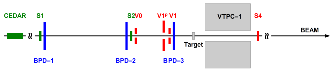
(a) Beam and trigger configuration

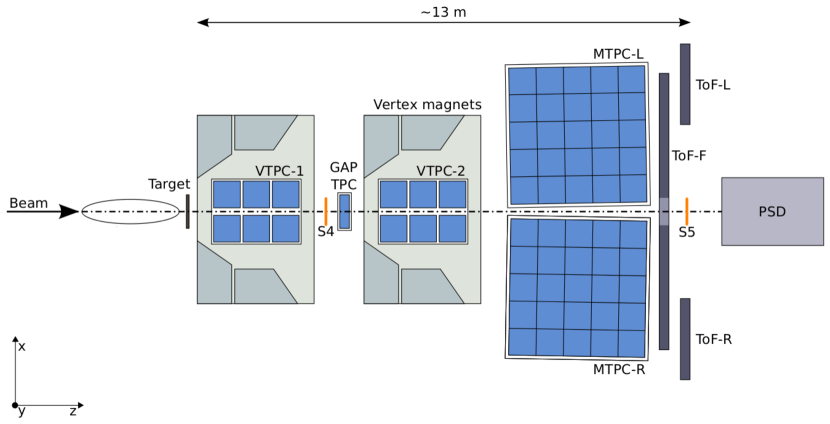
(b) Schematic layout in the beam plane

Figure 1: Experimental Setup of the NA61/SHINE experiment [30] (configuration for the $\pi^{-}$+C data taking). The coordinate system used in this paper is indicated on the lower left. The incoming beam direction is along the $z$ axis. The magnetic field bends charged particle trajectories in the $x{-}z$ (horizontal) plane. The drift direction in the TPCs is along the $y$ (vertical) axis. The beam and trigger instrumentation is indicated as an ellipse in the lower panel and detailed in the upper panel.

The magnet current setting for data taking at 158 and 350 $\mbox{Ge\kern-1.00006ptV}\kern-1.00006pt/\kern-0.50003ptc$ corresponds to 1.5 T in the first and 1.1 T, in the second magnet. It results in a precise measurement of the particle momenta $p$ with a resolution of $\sigma(p)/p^{2}\approx(0.3{-}7){\times}10^{-4}\,\mathrm{(GeV/c)}^{-1}$.

Two scintillation counters, S1 and S2, together with the three veto counters V0, V1 and V1${}^{\text{p}}$, define the beam upstream of the target. The setup of these counters can be seen in Fig. 1(a) for the 158 $\mbox{Ge\kern-1.00006ptV}\kern-1.00006pt/\kern-0.50003ptc$ run. The S1 counter also provides the start time for all timing measurements.

The 158 and 350 $\mbox{Ge\kern-1.00006ptV}\kern-1.00006pt/\kern-0.50003ptc$ secondary hadron beam was produced by 400 $\mbox{Ge\kern-1.00006ptV}\kern-1.00006pt/\kern-0.50003ptc$ primary protons impinging on a 10 cm long beryllium target. Negatively charged hadrons ($\text{h}^{-}$) produced at the target are transported downstream to the experiment by the H2 beamline, in which collimation and momentum selection occur. The beam particles, mostly $\pi^{-}$ mesons, are identified by a differential ring-imaging Cherenkov detector CEDAR [38]. The fraction of pions is ${\approx}95\%$ for 158 $\mbox{Ge\kern-1.00006ptV}\kern-1.00006pt/\kern-0.50003ptc$ and ${\approx}100\%$ for 350 $\mbox{Ge\kern-1.00006ptV}\kern-1.00006pt/\kern-0.50003ptc$ (see Fig. 2). The CEDAR signal is recorded during data taking and then used as an offline selection cut (see Sec. 3.1). The beam particles are selected by the beam trigger, T${}_{\text{beam}}$, then defined by the coincidence $\text{S1}\land\text{S2}\land\overline{\text{V0}}\land\overline{\text{V1}}\land\overline{\text{V1}^{\text{p}}}$. The interaction trigger ($\text{T}_{\text{int}}=\text{T}_{\text{beam}}\land\overline{\text{S4}}$) is given by the anti-coincidence of the incoming beam particle and S4, a scintillation counter, with a diameter of 2 cm, placed between the VTPC-1 and VTPC-2 detectors along the beam trajectory at about 3.7 m from the target, see Figs. 1(b) and 1(a). Almost all beam particles that interact inelastically in the target do not reach S4. The interaction and beam triggers were recorded in parallel. The beam trigger events were recorded with a frequency by a factor of about 10 lower than the frequency of interaction trigger events.

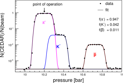
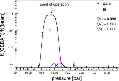
Figure 2: The fraction of CEDAR triggers as a function of its gas pressure for beam momenta of 158 (left) and 350 (right) $\mbox{Ge\kern-1.00006ptV}\kern-1.00006pt/\kern-0.50003ptc$. The fitted fractions $f$ of pions, kaons and anti-protons are quoted within the figures and the point of operation during data taking is indicated by an arrow.

The incoming beam trajectory is measured by a set of three Beam Position Detectors (BPDs), placed along the beamline upstream of the target, as shown in Fig. 1(a). These detectors are $4.8\times 4.8$ cm² proportional chambers. Each BPD measures the position of the beam particle on the transverse plane with respect to the beam direction with a resolution of ${\sim}100\,\upmu$m (see Ref. [30] for more details).

For data taking on $\pi^{-}$+C interactions, the target was an isotropic graphite plate with a thickness along the beam axis of 2 cm with a density of $\rho=1.84$ g/cm³, equivalent to about 4% of a nuclear interaction length. During the data taking the target was placed 80 cm upstream of VTPC-1. 90% of data was recorded with the target inserted and 10% with the removed target. The latter set was used to estimate the bias due to interactions with the material upstream and downstream of the target.

Detector parameters were optimised using a data-based calibration procedure which also took into account their time dependences. Minor adjustments were determined in consecutive steps for:

1. detector geometry and TPC drift velocities and

2. magnetic field map.

Each step involved reconstruction of the data required to optimise a given set of calibration constants and time dependent corrections followed by verification procedures. Details of the procedure and quality assessment are presented in Ref. [39].

The main steps of the data reconstruction procedure are:

1. finding of clusters in the TPC raw data, calculation of the cluster centre-of-gravity and total charge,

2. reconstruction of local track segments in each TPC separately,

3. matching of track segments into global tracks,

4. fitting of the track through the magnetic field and determination of track parameters at the first measured TPC cluster,

5. determination of the interaction vertex using the beam trajectory fitted in the BPDs and the trajectories of tracks reconstructed in the TPCs (the final data analysis uses the middle of the target as the $z$-position, $z=-580\,$cm) and

6. refitting of the particle trajectory using the interaction vertex as an additional point and determining the particle momentum at the interaction vertex.

An example of a reconstructed $\pi^{-}$+C interaction at 158 $\mbox{Ge\kern-1.00006ptV}\kern-1.00006pt/\kern-0.50003ptc$ is shown in Fig. 3. Amongst the many tracks visible are five long tracks of three negatively charged and two positively charged particles, with momentum ranging $5{-}50$ $\mbox{Ge\kern-1.00006ptV}\kern-1.00006pt/\kern-0.50003ptc$.

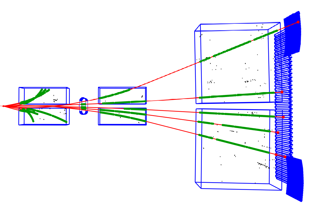
Figure 3: An example of a $\pi^{-}$+C interaction at 158 $\mbox{Ge\kern-1.00006ptV}\kern-1.00006pt/\kern-0.50003ptc$ measured in the detector (top view). The measured points (green dots) are used to fit tracks (red lines) to the interaction point. The black dots show the noise clusters and the red dots show matched Time of Flight hits (not used in this analysis).

A simulation of the detector response is used to correct the measured raw yields of resonances. For the purposes of this analysis, the Epos 1.99 model was used for the simulation and calculation of correction factors. DPMJet 3.06 [40] was used as a comparison for estimation of systematic uncertainties. The choice of Epos was made due to both the number of resonances included in the model, as well as the ability to include the intrinsic width of these resonances in the simulation. Epos 1.99 rather than Epos LHC was used as it is better tuned to the measurements at SPS energies [41].

The simulation consists of the following steps:

1. generation of inelastic $\pi^{-}$+C interactions using the Epos 1.99 model,

2. propagation of outgoing particles through the detector material using the Geant 3.21 package [42] which takes into account the magnetic field as well as relevant physics processes, such as particle interactions and decays,

3. simulation of the detector response using dedicated packages which also introduce distortions corresponding to all corrections applied to the real data,

4. simulation of the interaction trigger selection by checking whether a charged particle hits the S4 counter,

5. storage of the simulated events in a file which has the same format as the raw data,

6. reconstruction of the simulated events with the same reconstruction chain as used for the real data and

7. matching of the reconstructed to the simulated tracks based on the cluster positions.

For more details on the reconstruction and calibration algorithms applied to the raw data, as well as the simulation of the NA61/SHINE detector response, used to correct the raw data, see Ref. [43].

3 Analysis

In this section we present the analysis technique developed for the measurement of the $\rho^{0}$, $\omega$ and K^∗0 spectra in $\pi^{-}$+C production interactions. Production interactions are interactions with at least one new particle produced, i.e. interactions where only elastic or quasi-elastic scattering occurred are excluded. The procedure used for the data analysis consists of the following steps:

1. application of event and track selection criteria,

2. combination of oppositely charged tracks,

3. accumulating the combinations in bins of Feynman-$x$, $x_{\text{F}}$, calculated by using the mass of the $\rho^{0}$ meson for the boost between the lab and centre of mass frames,

4. calculation of the invariant mass of each combination, assuming pion masses for the particles,

5. fitting of the invariant mass distributions with templates of resonance decays to obtain raw yields and

6. application of corrections to the raw yields calculated from simulations.

These steps are described in the following subsections.

3.1 Event and track selection

A total of $5.49{\times}10^{6}$ events were recorded at 158 $\mbox{Ge\kern-1.00006ptV}\kern-1.00006pt/\kern-0.50003ptc$ and $4.48{\times}10^{6}$ events were recorded at 350 $\mbox{Ge\kern-1.00006ptV}\kern-1.00006pt/\kern-0.50003ptc$. All events used in the analysis are required to pass cuts to ensure both an interaction event and events of good quality. These cuts are:

1. Well-contained measurements of the beam with the BPDs and a successful reconstruction of the beam direction.

2. Pion identification with the CEDAR (only for 158 $\mbox{Ge\kern-1.00006ptV}\kern-1.00006pt/\kern-0.50003ptc$ as the impurity of the 350 $\mbox{Ge\kern-1.00006ptV}\kern-1.00006pt/\kern-0.50003ptc$ beam is below 0.1%).

3. No extra (off-time) beam particles detected within $\pm 2\,\upmu$s of the triggered beam particle.

4. All events must have an interaction trigger as defined in Sec. 2.

5. The main vertex point is properly reconstructed.

6. The $z$-position of the interaction vertex must be between $-597$ cm and $-563$ cm.

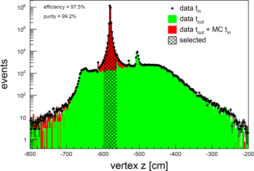
Figure 4: Distribution of fitted vertex $z$ positions for $\pi^{-}$+C interactions at 158 $\mbox{Ge\kern-1.00006ptV}\kern-1.00006pt/\kern-0.50003ptc$. The filled green area shows the distribution for events recorded with the target removed, while the filled red area shows the distribution for the reconstructed Monte Carlo simulation. The dashed area indicates events selected for this analysis.

The cut (vi) is illustrated in Fig. 4 and its purpose is to remove the majority of interactions that do not occur in the target. This cut will increase the Monte Carlo correction because some in-target events are removed due to the vertex $z$ resolution. However, as there is good agreement between the data and Monte Carlo vertex $z$ distributions, this will only have a minor impact on systematic uncertainties. An alternative method to correct for out-of-target interactions would be to measure the resonance yields in the target-removed data, but the template-fitting method used in this paper can not be applied to data sets with small statistics such as the target-removed data.

The range of this cut, ($-597,-563$) cm, was selected to maximise the event number, while minimising the contamination due to off-target events. The residual contribution of non-target interactions after applying this cut is 0.8%.

Table 1: Number of events after each event selection cut and selection efficiency with respect to the previous cut for the target inserted data set for 158 $\mbox{Ge\kern-1.00006ptV}\kern-1.00006pt/\kern-0.50003ptc$ and 350 $\mbox{Ge\kern-1.00006ptV}\kern-1.00006pt/\kern-0.50003ptc$ beam momentum.

	$p_{\text{beam}}$	$158\,\mbox{Ge\kern-1.00006ptV}\kern-1.00006pt/\kern-0.50003ptc$		$350\,\mbox{Ge\kern-1.00006ptV}\kern-1.00006pt/\kern-0.50003ptc$
	Cut	$N_{\text{events}}$	Efficiency (%)	$N_{\text{events}}$	Efficiency (%)
	Total	$5.49{\times}10^{6}$	100	$4.48{\times}10^{6}$	100
(i)	BPD	$4.96{\times}10^{6}$	90.3	$4.08{\times}10^{6}$	91.1
(ii)	CEDAR	$4.26{\times}10^{6}$	85.9	$4.08{\times}10^{6}$	100
(iii)	Off-time	$4.03{\times}10^{6}$	94.5	$3.94{\times}10^{6}$	96.5
(iv)	Trigger	$3.34{\times}10^{6}$	83.0	$2.97{\times}10^{6}$	75.3
(v)	Vertex fit	$3.29{\times}10^{6}$	98.5	$2.95{\times}10^{6}$	99.5
(vi)	$z$-position	$2.78{\times}10^{6}$	84.6	$2.59{\times}10^{6}$	87.9

Table 2: Number of tracks after each track selection cut and selection efficiency with respect to the previous cut for the target inserted data set for 350 $\mbox{Ge\kern-1.00006ptV}\kern-1.00006pt/\kern-0.50003ptc$ beam momentum.

	$p_{\text{beam}}$	$158\,\mbox{Ge\kern-1.00006ptV}\kern-1.00006pt/\kern-0.50003ptc$		$350\,\mbox{Ge\kern-1.00006ptV}\kern-1.00006pt/\kern-0.50003ptc$
	Cut	$N_{\text{tracks}}$	Efficiency (%)	$N_{\text{tracks}}$	Efficiency (%)
	Total	$3.85{\times}10^{7}$	100	$4.41{\times}10^{7}$	100
(i)	Track quality	$2.27{\times}10^{7}$	59.0	$2.77{\times}10^{7}$	62.8
(ii)	Acceptance	$1.57{\times}10^{7}$	69.0	$1.99{\times}10^{7}$	72.0
(iii)	Total clusters	$1.54{\times}10^{7}$	98.1	$1.95{\times}10^{7}$	98.2
(iv)	TPC clusters	$1.51{\times}10^{7}$	98.0	$1.91{\times}10^{7}$	97.8
(v)	Impact parameters	$1.42{\times}10^{7}$	94.4	$1.80{\times}10^{7}$	94.1

The number of events after these cuts is $2.78{\times}10^{6}$ for 158 $\mbox{Ge\kern-1.00006ptV}\kern-1.00006pt/\kern-0.50003ptc$ and $2.59{\times}10^{6}$ for 350 $\mbox{Ge\kern-1.00006ptV}\kern-1.00006pt/\kern-0.50003ptc$. The efficiency of these cuts is shown in Table 1 for 158 $\mbox{Ge\kern-1.00006ptV}\kern-1.00006pt/\kern-0.50003ptc$ and 350 $\mbox{Ge\kern-1.00006ptV}\kern-1.00006pt/\kern-0.50003ptc$ beam momentum.

After the event cuts were applied, a further set of quality cuts were applied to the individual tracks. These were used to ensure a high reconstruction efficiency as well as reducing contamination by tracks from secondary interactions. These cuts are:

1. The track is well reconstructed at the interaction vertex.

2. The fitted track is inside the geometrical acceptance of the detector.

3. The total number of clusters on the track should be greater than or equal to 30.

4. The sum of clusters on the track in VTPC-1 and VTPC-2 should be greater than or equal to 15, or the total number of clusters on the track in GTPC should be greater than or equal to 6.

5. The distance of closest approach of the fitted track to the interaction point (impact parameter) is required to be less than 2 cm in the $x$-plane and 0.4 cm in the $y$-plane.

For the acceptance cut, (ii), we studied the selection efficiency with simulations as a function of azimuthal angle $\phi$ for bins in total momentum $p$ and transverse momentum $p_{\text{T}}$. This leads to a three-dimensional lookup table that defines the regions in $(\phi,p,p_{\text{T}})$ for which the selection efficiency is larger than 90%. Within this region, the detector is close to fully efficient and the corresponding correction factor is purely geometric, since the production of resonances is uniform in $\phi$ for an unpolarised beam and target.

The efficiency of each track-selection cut is shown in Table 2 for the data collected at 158 $\mbox{Ge\kern-1.00006ptV}\kern-1.00006pt/\kern-0.50003ptc$ and 350 $\mbox{Ge\kern-1.00006ptV}\kern-1.00006pt/\kern-0.50003ptc$.

No particle identification was used in this analysis. This increases the background but simplifies the analysis and increases the longitudinal momentum range of the results. The longitudinal momentum fraction, $x^{\prime}_{\text{F}}$, was calculated as

$$x^{\prime}_{\text{F}}=\frac{2p_{\text{L}}}{\sqrt{s}}\quad\left(\approx\frac{p_{\text{L}}}{p_{\text{L}}(\mathrm{max})}\right),$$ (1)

where $p_{\text{L}}$ is the longitudinal momentum of the $\rho^{0}$-candidate in the centre of mass frame in the pion-nucleon interaction and $\sqrt{s}$ is the centre of mass energy of the interaction. $p_{\text{L}}$ is calculated using the mean mass of the $\rho^{0}$ meson ($m_{\rho^{0}}=0.775\,\mbox{Ge\kern-1.00006ptV}\kern-1.00006pt/\kern-0.50003ptc^{2}$) when boosting between the lab frame and the centre of mass frame. The mass of the nucleon used in the calculations is taken to be the average of the proton and neutron masses. There is no difference between $x^{\prime}_{\text{F}}$ and the Feynman-$x$, $x_{\text{F}}=p_{\text{L}}/p_{\text{L}}(\text{max})$, for a particle pair originating from a $\rho^{0}$ meson decay. For $\omega$ or K^∗0 decays the difference is less than 0.01 in the $x^{\prime}_{\text{F}}$ range covered by the results presented here. This difference approaches zero with increasing $x^{\prime}_{\text{F}}$. For simplicity, in the following, $x^{\prime}_{\text{F}}$ is denoted as $x_{\text{F}}$.

3.2 Signal extraction

The raw yields of $\rho^{0}$, $\omega$ and K^∗0 mesons were obtained by performing a fit of inclusive invariant mass spectra. These were calculated by assuming every track that passes the cuts is a charged $\pi$. Then, for all pairs of positively and negatively charged particles, the invariant mass was calculated assuming pion masses for both particles. Examples of invariant mass spectra at 158 $\mbox{Ge\kern-1.00006ptV}\kern-1.00006pt/\kern-0.50003ptc$ and 350 $\mbox{Ge\kern-1.00006ptV}\kern-1.00006pt/\kern-0.50003ptc$ are shown in Fig. 5.

In the inclusive invariant mass spectra, there is a large combinatorial background, especially at low $x_{\text{F}}$. The method used to estimate the background is the so-called charge mixing method, which uses the invariant mass spectra calculated exactly as explained above, but using same-charge instead of opposite-charge tracks. The resulting charge mixing background spectra are shown in Fig. 5. As the normalisation of these spectra will differ from the true background, the normalisation of the charge-mixed spectra is included as a parameter in the fit to the data. The uncertainty introduced by choosing this method of calculating the background is estimated by comparing it with a background found from simulations. This Monte Carlo background is defined as the sum of:

• combinations of tracks that come from decays of different resonances, i.e. one track from a $\rho^{0}$ and one from an $\omega$ (this can be done as the parent particles of tracks are known in the simulation),

• combinations of tracks coming directly from the interaction vertex and

• combinations of tracks coming from resonances (both meson and baryon) that are not included in the individual fitting-templates listed below.

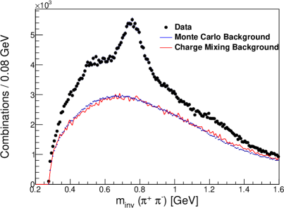
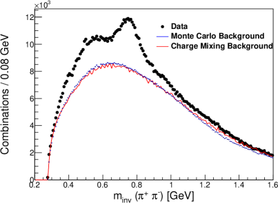
Figure 5: Invariant mass distribution of opposite charge particles, calculated assuming pion masses, in $\pi^{-}$+C production interactions at 158 $\mbox{Ge\kern-1.00006ptV}\kern-1.00006pt/\kern-0.50003ptc$ in the range $0.4<x_{\text{F}}<0.5$ (left) and $0.3<x_{\text{F}}<0.4$ (right). The background estimated through the charge mixing method is shown in red and the background from the simulation is shown in blue.

As can be seen in Fig. 5, there is a good overall agreement between the two background estimation methods and the residual differences are used to estimate the systematics due to background subtraction. The boundaries of the default fit range are chosen to include all resonances of interest and to select the invariant mass region for which there is good agreement between the two background estimates, and hence the results have small systematic biases. This leads to the fit range in $m_{\text{inv}}(\pi^{+}\pi^{-})$ of $0.475{-}1.35\,\mbox{Ge\kern-1.00006ptV}\kern-1.00006pt/\kern-0.50003ptc^{2}$.

Event mixing was also investigated as an alternative way to estimate the background by taking particles from different events to make invariant mass spectra of $\pi^{+}\pi^{-}$ candidates, but this method was found to not describe the shape of the background in simulations over the mass range of the $\rho^{0}$, $\omega$ and K^∗0 distributions needed to obtain reliable fit results. Refining the event mixing method by splitting the data into multiplicity classes did not improve the quality of this method.

As there is a large number of resonances in the $m_{\text{inv}}(\pi^{+}\pi^{-})$ region around the mass of the $\rho^{0}$, such as the $\omega$ and K^∗0 mesons, they all have to be taken into account. This has previously been shown in Ref. [44], where only taking into account $\rho^{0}$ and $\omega$ mesons resulted in an inadequate fit, with a spurious peak at 0.6 $\mbox{Ge\kern-1.00006ptV}\kern-1.00006pt/\kern-0.50003ptc^{2}$ in the $\pi^{+}\pi^{-}$ invariant mass spectra, due to decays of K^∗0 mesons, where the kaon is assigned the mass of a pion. As there is no particle identification used in this analysis, the effect due to K^∗0 meson production is expected to be strong and it must be included in the fitting procedure. Other contributions that are not represented by an individual template, such as $\Lambda$ decay products, are included in the Monte Carlo background.

The fitting procedure uses templates of the invariant mass distribution for each resonance of importance. This method of template fitting is similar to ideas used by many other experiments such as ALICE [45], ATLAS [46], CDF [47] and CMS [48], where it is also known as the cocktail fit method. The templates are constructed by passing simulated $\pi^{-}$+C production interactions, generated with the Epos 1.99 [12] hadronic interaction model using Crmc 1.5.3 [49], through the full detector Monte Carlo chain and then through the same reconstruction routines as the data. Crmc is an event generator package with access to a variety of different event generators, such as DPMJet 3.06 [40] and Epos LHC [50].

The template method also allows for the fitting of resonances with dominant three body decays, such as $\omega$, as well as resonances with two-body non-$\pi^{+}\pi^{-}$ decays, such as K^∗0. A list of all decays with a branching ratio of over $1\%$ that are used in the templates is shown in Table 3. The templates and the data are split into bins of $x_{\text{F}}$, calculated as in Eq. 1.

Table 3: Decays of resonances for which $m_{\text{inv}}(\pi^{+}\pi^{-})$ templates were calculated and fitted. Only decays with a branching ratio greater than 1% into at least one positively and one negatively charged particle are considered. Branching ratios were taken from [51]

.

Resonance	Decay	Branching ratio
$\rho^{0}$	$\pi^{+}\pi^{-}$	100.0
$\omega$	$\pi^{+}\pi^{-}\pi^{0}$	89.1
	$\pi^{+}\pi^{-}$	1.53
K∗0	K $\pi$	100.0
f2	$\pi^{+}\pi^{-}$	57.0
	$\pi^{+}\pi^{-}\,2\pi^{0}$	7.7
	K+K-	4.6
	$2\pi^{+}\,2\pi^{-}$	2.8
$\eta$	$\pi^{+}\pi^{-}\pi^{0}$	22.7
	$\pi^{+}\pi^{-}\gamma$	4.6
f0 (980)	$\pi^{+}\pi^{-}$	50.0
	K+K-	12.5
a2	$3\pi$	70.1
	$\eta\,\pi$	14.5
	$\omega\,\pi\,\pi$	10.6
	K $\bar{\text{K}}$	4.9
$\rho_{3}$	$4\pi$	71.1
	$\pi\,\pi$	23.6
	K K $\pi$	3.8
	K $\bar{\text{K}}$	1.58
K${}^{0}_{\text{S}}$	$\pi^{+}\pi^{-}$	69.20

The templates in the fit are the charge mixing background and the following resonances: $\rho^{0}$, K^∗0, $\omega$, f₂, f₀ (980), a₂, $\rho_{3}$, $\eta$ and K${}^{0}_{\text{S}}$. The templates were generated from reconstructed simulations that have all the standard reconstruction cuts applied; they include effects due to the resolution of the detector and the fiducial acceptance. The templates used in the fits are presented in App. B. As can be seen, the a₂ and $\rho_{3}$ templates are broad and featureless similar to the background template. For this reason, these resonances cannot be fitted reliably and will be subtracted together with the background from figures displaying the result of the template fitting in the following.

The fit to the $\pi^{+}\pi^{-}$ mass spectrum is performed between masses of 0.475 $\mbox{Ge\kern-1.00006ptV}\kern-1.00006pt/\kern-0.50003ptc^{2}$ and 1.35 $\mbox{Ge\kern-1.00006ptV}\kern-1.00006pt/\kern-0.50003ptc^{2}$ using the expression

$$\mu(m_{\text{inv}})=\sum_{i}f_{i}\,T_{i}(m_{\text{inv}}),$$ (2)

where $f_{i}$ is the contribution for particle $i$, $T_{i}$ is the associated invariant mass template and $m_{\text{inv}}$ is the invariant mass. $f_{i}$ is constrained to be between 0 and 1. The templates are normalised to the same number of combinations as the data over the range of the fit. The fit uses a standard Poissonian likelihood function

$$\mathcal{L}=\prod_{j}\frac{\mu_{j}^{k_{j}}e^{-\mu_{j}}}{k_{j}!},$$ (3)

where $k_{j}$ is the actual number of combinations in the invariant mass bin $j$ and $\mu_{j}$ is the expected number of combinations, taken from Eq. (2).

Two examples of the template-fitting are shown in Fig. 6 for 158 $\mbox{Ge\kern-1.00006ptV}\kern-1.00006pt/\kern-0.50003ptc$ and 350 $\mbox{Ge\kern-1.00006ptV}\kern-1.00006pt/\kern-0.50003ptc$. The fitted charge-mixing background as well as the contribution of the featureless a₂ and $\rho_{3}$ resonances are subtracted to highlight the different resonances. The full set of template fits are displayed in App. C for all $x_{\text{F}}$-bins and the two beam energies.

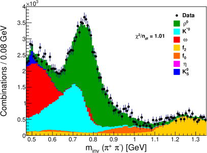
Figure 6: Invariant mass distribution of oppositely charged particles, calculated assuming pion masses, in $\pi^{-}$+C production interactions in the range $0.3<x_{\text{F}}<0.4$ at 158 $\mbox{Ge\kern-1.00006ptV}\kern-1.00006pt/\kern-0.50003ptc$ (left) and at 350 $\mbox{Ge\kern-1.00006ptV}\kern-1.00006pt/\kern-0.50003ptc$ (right). Dots with error bars denote the data and the fitted resonance templates are shown as filled histograms. The fitted background and featureless resonances have been subtracted.

After the fractions of each templates have been determined in the fit, the raw mean multiplicity $n_{i}$ of meson $i$ per event in a given $x_{\text{F}}$ bin is determined from

$$n_{i}(x_{\text{F}})=\frac{1}{N_{\text{acc}}}\sum_{j}f_{i}\,T_{i}(j),$$ (4)

where $N_{\text{acc}}$ is the number of events after selection cuts, $f_{i}$ is the result of the fit and $T_{i}$ is the template of the meson of interest $i$, e.g. $\rho^{0}$.

3.3 Correction factors

In order to obtain the true number of $\rho^{0}$, $\omega$ and K^∗0 mesons produced in $\pi^{-}$+C production interactions, three different corrections were applied to the raw yields. These corrections were calculated using 20 million events generated by the Epos 1.99 model using the Crmc package.

1. The Monte Carlo simulations that were used to obtain the templates for the fitting procedure were used to calculate corrections due to geometrical acceptance, reconstruction efficiency, losses due to trigger bias, quality cuts and bin migration effects. For each $x_{\text{F}}$ bin, the correction factor $C(x_{\text{F}})$ is given by

   $$C(x_{\text{F}})=\frac{n_{\text{MC}}^{\text{gen}}(x_{\text{F}})}{n_{\text{MC}}^{\text{acc}}(x_{\text{F}})},$$ (5)

   where

   1. $n_{\text{MC}}^{\text{gen}}(x_{\text{F}})$ is the mean multiplicity per event of $\rho^{0}$ ($\omega$, K^∗0) mesons produced in a given $x_{\text{F}}$ bin in $\pi^{-}$+C production interactions at a given beam momentum, including $\rho^{0}$ ($\omega$, K^∗0) mesons from higher mass resonance decays and

   2. $n_{\text{MC}}^{\text{acc}}(x_{\text{F}})$ is the mean multiplicity per event of reconstructed $\rho^{0}$ ($\omega$, K^∗0) mesons that are accepted after applying all event and track cuts.

   The statistical uncertainties of the corrections factors were calculated assuming binomial distributions for the number of events and resonances.

2. The contribution from $\rho^{0}$ mesons produced by re-interactions in the target. This was estimated from the simulations. This contribution is less than 1% for all bins apart from $x_{\text{F}}<0.15$, where the contribution is 1.7%.

3. The fitting method was validated by applying the same procedure to the simulated data set, using the background estimated from either the charge mixing method or the true background obtained from the simulation. This difference is then applied as a multiplicative correction to the raw yield, $f_{i}^{\text{true}}/f_{i}^{\text{fit}}$, where $f_{i}^{\text{true}}$ is the true yield of resonance $i$ and $f_{i}^{\text{fit}}$ is the yield that comes from the fit to the simulations. This correction is calculated separately for both background estimations and applied to the fits to the data that used the same estimation.

The breakdown of these correction factors can be seen, for the $\rho^{0}$ spectra at $p_{\text{beam}}=158$ and $350\,\mbox{Ge\kern-1.00006ptV}\kern-1.00006pt/\kern-0.50003ptc$, in Fig. 7. The correction factor $C(x_{\text{F}})$ is broken down into three contributions: bias from the interaction trigger (T2), geometrical acceptance, and selection efficiency. The geometrical acceptance dominates for large $x_{\text{F}}$ values.

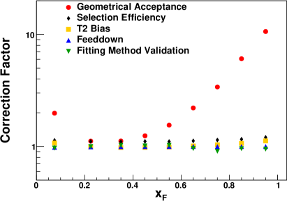
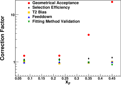
Figure 7: Correction factors for the $\rho^{0}$ spectra in $\pi^{-}$+C production interactions at 158 $\mbox{Ge\kern-1.00006ptV}\kern-1.00006pt/\kern-0.50003ptc$ (left) and 350 $\mbox{Ge\kern-1.00006ptV}\kern-1.00006pt/\kern-0.50003ptc$ (right). It can easily be seen that the correction for geometrical acceptance dominates in almost every bin.

The correction derived from Monte Carlo simulations could introduce a bias in the result if the $p_{\text{T}}$ spectrum of the model differed from the true shape. This is because the extrapolation to full $p_{\text{T}}$ phase space is based on the model spectrum. To investigate this effect another hadronic interaction model was used, DPMJet 3.06 [40]. This model also provides $p_{\text{T}}$ spectra for each resonance measured in this analysis, and the difference between the correction factors found for DPMJet 3.06 and Epos 1.99 is less than 4%. This suggests that any bias introduced by the extrapolation to full $p_{\text{T}}$ phase space is small. The difference between the correction factors is used in the estimate of the systematic uncertainties.

The final measurement is calculated by taking the average of the result using the two different background description methods, charge mixing and Monte Carlo background, with all the correction factors that change calculated separately for the two methods. The difference between these two methods is taken to be a systematic uncertainty.

3.4 Uncertainties and Cross Checks

The statistical uncertainties in the $i$th $x_{\text{F}}$-bin are given by

$$\sigma_{i}^{2}=\left(\Delta C_{i}\,n_{i}\right)^{2}+\left(\frac{\sigma(n_{i})}{C_{i}}\right)^{2},$$ (6)

where $n_{i}$ and $\sigma(n_{i})$ are the raw meson mean multiplicity per event and the uncertainty on this multiplicity that comes from the template fit. The contribution due to the uncertainty of the meson multiplicity dominates as the uncertainty $\Delta C_{i}$ of the corrections factors is only from the statistics of the simulation (20 million events) which is much larger than that of the data.

The main contributors to the systematic uncertainties are

1. The fitting method used for estimating the background shape and the fit procedure. The systematic uncertainty is taken to be half the difference between the two methods, using either charge mixing or Monte Carlo background, after the respective validation corrections have been applied. This estimate therefore combines the systematic uncertainty due to both the fitting method validation correction and the background estimation used and this is the dominant systematic uncertainty.

2. Correction factors. The correction factors calculated above were compared with factors found using a different hadronic interaction model, DPMJet 3.06.

3. Track cuts. The effect of the event and track selection cuts were checked by performing the analysis with the following cuts changed, compared to the values shown in Sec. 3.1.

   1. The cut on the $z$-position of the interaction vertex was changed to be between $-590$ cm and $-570$ cm.

   2. The window in which off-time beam particles were not allowed was decreased from 2 $\upmu$s to 1.5 $\upmu$s.

   3. The minimum number of clusters on the track was decreased to 25.

   4. The sum of clusters on the track in VTPC-1 and VTPC-2 was decreased to 12 or increased to 18.

   5. The impact parameter cuts were increased to less than 4 cm in the $x$-plane and 2 cm in the $y$-plane.

The systematic uncertainties were estimated from the differences between the results obtained using the standard analysis and ones obtained when adjusting the method as listed above. The individual systematic uncertainties were added in quadrature to obtain the total systematic uncertainties. They are dominated by the correction factor contribution, up to 15%, whereas the other contributions are less than 4%. Other sources of uncertainty, such as using templates from a different model, are found to be much smaller.

The fraction of target removed tracks is less than $0.15\%$ in all $x_{\text{F}}$ bins. The shape of the target removed distributions, after applying all the track and event cuts, is consistent with the background description so there is no additional correction or systematic uncertainty considered.

Several cross checks were performed to validate the results and check their stability. These include extending the range of the $m_{\text{inv}}(\pi^{+}\pi^{-})$ fit, using the Breit-Wigner function to describe the $\rho^{0}$ instead of a template as well as a few other more simple checks.

3.4.1 Fit range

The default fit range used in this analysis was restricted to the mass ranges of the resonances of interest. We tested an extended fit range by including all data down to the kinematic threshold of $m_{\text{inv}}(\pi^{+}\pi^{-})=2m_{\pi}$. For this purpose additional templates needed to be taken into account including electrons and positrons pair-produced in the target by photons from $\pi^{0}$ decays. The sum of all resonances produced by the Epos 1.99 model can however not describe the low $m_{\text{inv}}(\pi^{+}\pi^{-})$ region satisfactorily. In particular, a significant bump at a mass of ${\approx}0.4\,\mbox{Ge\kern-1.00006ptV}\kern-1.00006pt/\kern-0.50003ptc^{2}$ appears to be in the data that does not have a counterpart in the templates. No resonance, meson or baryon, could be found in Epos 1.99 that could describe this bump. To avoid any bias the region of $0.35\,\mbox{Ge\kern-1.00006ptV}\kern-1.00006pt/\kern-0.50003ptc^{2}<m_{\text{inv}}(\pi^{+}\pi^{-})<0.4\,\mbox{Ge\kern-1.00006ptV}\kern-1.00006pt/\kern-0.50003ptc^{2}$ was excluded from the fit. Further discussions about the study of this bump are given in App. D.

Once this region is excluded from the fit a reasonable description of the $m_{\text{inv}}$ distribution down to the kinematic limit can be achieved, as shown in Fig. 8. However, the fit quality is worse and the agreement between the two background estimates is weaker. The poorer fit quality is most likely a combination of poorer performance of the estimate of the combinatorial background close to the kinematic threshold and the missing template to describe the bump at ${\approx}0.375\,\mbox{Ge\kern-1.00006ptV}\kern-1.00006pt/\kern-0.50003ptc^{2}$.

The yields obtained with the extended range differ by less than the systematic uncertainties from the yields with the original range, with the exception of one bin, and, to be conservative, the corresponding differences, which are of the order of 10%, are included in the systematic uncertainty.

Figure 8: An example of the template fit to 158 $\mbox{Ge\kern-1.00006ptV}\kern-1.00006pt/\kern-0.50003ptc$ data in the range $0.3<x_{\text{F}}<0.4$ using the nominal fit range (left) and the extended fit range (right) including a template for $e^{+}e^{-}$ pair production.

3.4.2 $\rho^{0}$ mass

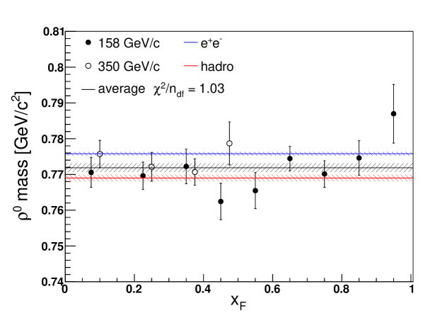
Figure 9: Fitted $\rho^{0}$ mass for $\pi^{-}$+C production interactions as a function of $x_{\text{F}}$. The blue line indicates the average mass from $e^{+}e^{-}$ annihilation and the red line indicates the average mass from other reactions, which is dominated by hadroproduction measurements [51]. The black line is the weighted mean of all measurements, combining both 158 and 350 $\mbox{Ge\kern-1.00006ptV}\kern-1.00006pt/\kern-0.50003ptc$ data.

We checked for possible nuclear effects on the $\rho^{0}$ mass [52, 53] by removing the $\rho^{0}$ template from the fit and replacing it with a Breit-Wigner function. The function used is the one used in Ref. [54] with a modification to the decay width following Refs. [55] and [56], where the decay width is a function of mass $m_{\text{inv}}$,

$$\operatorname{BW}(m_{\text{inv}})=\frac{m_{\text{inv}}\,m_{\text{R}}\,\Gamma}{(m_{\text{R}}^{2}-m_{\text{inv}}^{2})^{2}+m_{\text{R}}^{2}\,\Gamma^{2}},$$ (7)

where $m_{\text{R}}$ is the mean mass of the fitted resonance and $\Gamma$ is given by

$$\Gamma(m_{\text{inv}})=\Gamma_{0}\left(\frac{m_{\text{R}}}{m_{\text{inv}}}\right)\left(\frac{q}{q_{\text{R}}}\right)^{3/2}\left(\frac{q_{\text{R}}^{2}+\delta^{2}}{q^{2}+\delta^{2}}\right),$$ (8)

where $q$ and $q_{\text{R}}$ are the pion three-momenta in the rest frame of the resonance, calculated with mass $m_{\text{inv}}$ and $m_{\text{R}}$, respectively. The parameter $\delta$ in the cutoff function has a value $\delta=0.3\,\mbox{Ge\kern-1.00006ptV}\kern-1.00006pt/\kern-0.50003ptc$.

We considered the mass as a free parameter and fixed the width value to the one provided by the particle data group [51]. The obtained mass values are consistent with the values quoted by the particle data group as shown in Fig. 9. The weighted average of the fitted masses is $0.772\pm 0.001\,\mbox{Ge\kern-1.00006ptV}\kern-1.00006pt/\kern-0.50003ptc^{2}$, with no significant difference between the 158 and 350 $\mbox{Ge\kern-1.00006ptV}\kern-1.00006pt/\kern-0.50003ptc$ data.

A simpler Breit-Wigner function was also tested,

$$\operatorname{BW}(M)=\frac{\Gamma^{2}}{(M-m_{\text{R}})^{2}+\Gamma^{2}}$$ (9)

It is the function used to both sample resonances and generate their widths in Epos 1.99. Even though this function does not directly take into account effects which are considered in the event generator, such as decay products approaching the lower kinematic limit, or energy conservation for decay products at higher mass, the resulting fitted masses are compatible with the results from the more complicated Breit-Wigner function, Eq. (7).

The yields of the $\rho^{0}$ when fitting with this Breit-Wigner function differ slightly from the yields calculated using the standard analysis method. These small differences of the order of 3% are included in the systematic uncertainties.

A comparison of the yields from the standard template analysis method, the extended fit range and when fitting a Breit-Wigner function (Eq. (7)) is shown in Fig. 10. As can be seen the differences are within the systematic uncertainties of the standard analysis. These small differences, of the order of 3% for the fits with a Breit-Wigner function and 10% for the extended fit range, are added in quadrature to the systematic uncertainties.

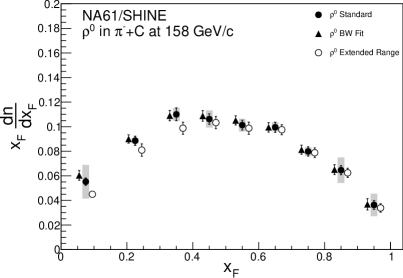
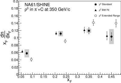
Figure 10: Comparison of $\rho^{0}$ $x_{\text{F}}$ spectra at 158 $\mbox{Ge\kern-1.00006ptV}\kern-1.00006pt/\kern-0.50003ptc$ (left) and 350 $\mbox{Ge\kern-1.00006ptV}\kern-1.00006pt/\kern-0.50003ptc$ (right) from the standard template analysis method, the extended fit range and when using a Breit-Wigner function to parameterise the $\rho^{0}$. The systematic uncertainties shown are before adding contributions from the differences to the extended fit range and Breit-Wigner function fits.

3.4.3 Further checks

Further cross checks were performed to probe the stability of the fit and yield result. These include

1. The data, along with the templates, were split into two equally sized regions of polar angle. If there was any polar-angle dependence of the result introduced by insufficient modeling of different parts of the detector, this would appear in a difference between the spectra from these independent data sets. The resulting multiplicity spectra were consistent within statistical uncertainties.

2. The data set was split according to different time ranges, both a night and day split as well as a first half and second half split in run taking. Any possible systematic differences in the detector which depend on time would result in discrepancies in the spectra from the different time ranges. Both resulting $x_{\text{F}}$ spectra were again consistent within statistical uncertainties.

3. Instead of assuming the pion mass for both tracks, one track was allocated the kaon mass. This means that the number of combinations used has to double, as both combinations of masses have to be taken into account for any given pair of tracks to allow for the kaon to be either of the two charges. This also then increases the background even further and because of the different shape of the background under the $\pi$ K invariant mass distribution, the systematic uncertainty for this method is larger than for the $\pi\,\pi$ method. The multiplicity spectra from this method were consistent within statistical and systematic uncertainties of the standard analysis method.

All these performed cross checks gave results consistent within the total uncertainties of the standard analysis.

4 Results

The yields of $\rho^{0}$, $\omega$, and K^∗0 mesons in $\pi^{-}$+C production interactions at 158 $\mbox{Ge\kern-1.00006ptV}\kern-1.00006pt/\kern-0.50003ptc$ and 350 $\mbox{Ge\kern-1.00006ptV}\kern-1.00006pt/\kern-0.50003ptc$ were calculated in bins of $x_{\text{F}}$ as follows

$$\frac{\mathrm{d}n}{\mathrm{d}x_{\text{F}}}=\frac{1}{N_{\text{prod}}}\frac{\mathrm{d}N_{\text{part}}}{\mathrm{d}x_{\text{F}}}=\frac{C(x_{\text{F}})\,n(x_{\text{F}})}{\Delta x_{\text{F}}},$$ (10)

where $N_{\text{prod}}$ is the number of interaction events minus the events with elastic and quasi-elastic scattering (which are not included), $N_{\text{part}}$ is the true number of produced resonances, $n(x_{\text{F}})$ is the raw mean multiplicity per event of the meson from Eq. (4), $\Delta x_{\text{F}}$ is the width of the $x_{\text{F}}$ bin and $C(x_{\text{F}})$ is the total correction factor for losses of event and multiplicity, as detailed above. Measured points with large statistical or systematic uncertainties (greater than 50%) are not shown. This cut removes three data points at large $x_{\text{F}}$ for the $\omega$ spectrum and one data point at large $x_{\text{F}}$ for the K^∗0 spectrum at 158 $\mbox{Ge\kern-1.00006ptV}\kern-1.00006pt/\kern-0.50003ptc$. In case of the data taken at $350\,\mbox{Ge\kern-1.00006ptV}\kern-1.00006pt/\kern-0.50003ptc$ only a limited $x_{\text{F}}$-range between 0 and 0.5 is accessible within the acceptance of . Only one data point of the $\omega$ spectrum survived the cut on the maximum uncertainty and none for the K^∗0 spectrum. Therefore we present only $\rho^{0}$ spectra for the $350\,\mbox{Ge\kern-1.00006ptV}\kern-1.00006pt/\kern-0.50003ptc$ data.

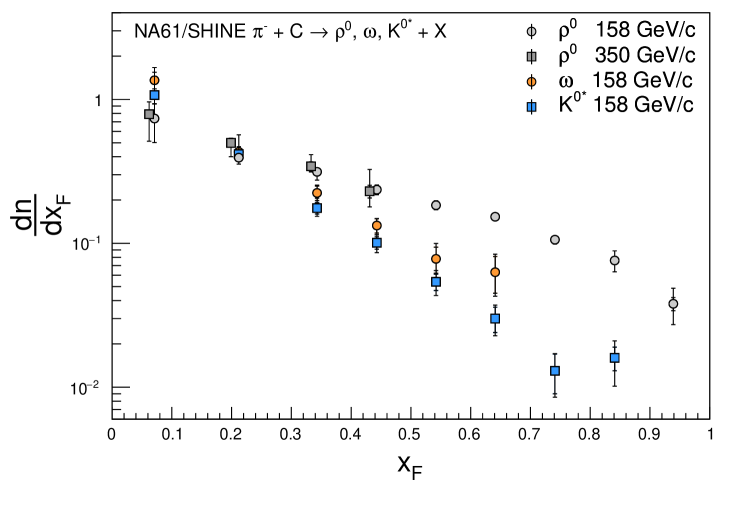
Figure 11: Average multiplicity of meson resonances in $\pi^{-}$+C collisions. The results for $\rho^{0}$ mesons are shown for $p_{\text{beam}}=158$ and 350 $\mbox{Ge\kern-1.00006ptV}\kern-1.00006pt/\kern-0.50003ptc$ and the spectra of $\omega$ and K^∗0 mesons were measured at $p_{\text{beam}}=158$ $\mbox{Ge\kern-1.00006ptV}\kern-1.00006pt/\kern-0.50003ptc$. The inner error bars show the statistical uncertainty and the outer error bar denotes the total uncertainty obtained by adding statistical and systematic uncertainties in quadrature.

The spectra of $\rho^{0}$, $\omega$, and K^∗0 mesons produced in production $\pi^{-}$+C interactions are shown in Fig. 11. The average $x_{\text{F}}$ in each bin is used to display the data points in this and in the following figures. It is worthwhile noting that this average is not corrected for the detector acceptance within the bin and is calculated from all oppositely charge combinations including combinatorial background. For a detailed comparison of this data with model predictions it is therefore recommended to compare to model predictions binned in the same way as the data rather than comparing them at the average $x_{\text{F}}$.

As can be seen in Fig. 11, no dependence of the $\rho^{0}$ multiplicities on beam energy was found within the uncertainties of the measurement. Out of the three resonances studied here, the multiplicity of $\rho^{0}$ mesons is the largest at large $x_{\text{F}}$, i.e. the region most relevant for the development of cosmic-ray air showers. Numerical results, including statistical and systematic uncertainties, are given in Tables 4, 5, and 6. It is worthwhile noting that due to improvements in the analysis procedure the final $\rho^{0}$ multiplicities at 158 $\mbox{Ge\kern-1.00006ptV}\kern-1.00006pt/\kern-0.50003ptc$ listed in Tab. 4 are about 25% smaller than the preliminary results presented in [33].

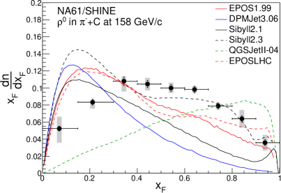
Figure 12: Scaled $x_{\text{F}}$-spectra of $\rho^{0}$ mesons, $x_{\text{F}}\,\mathrm{d}n/\mathrm{d}x_{\text{F}}$, in $\pi^{-}$+C production interactions at 158 (left) and $350\,\mbox{Ge\kern-1.00006ptV}\kern-1.00006pt/\kern-0.50003ptc$ (right). The error bars show the statistical, the bands indicate systematic uncertainties. The lines depict predictions of hadronic interaction models: red – Epos 1.99, blue – DPMJet 3.06, black – Sibyll 2.1, dashed green – QGSJet II-04, dashed red – Epos LHC, dashed black – Sibyll 2.3.

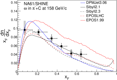
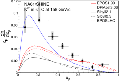
Figure 13: Scaled $x_{\text{F}}$-spectra of $\omega$ (left) and K^∗0 (right) mesons, $x_{\text{F}}\,\mathrm{d}n/\mathrm{d}x_{\text{F}}$, in $\pi^{-}$+C production interactions at $158\,\mbox{Ge\kern-1.00006ptV}\kern-1.00006pt/\kern-0.50003ptc$. The error bars show the statistical, the bands indicate systematic uncertainties. The lines depict predictions of hadronic interaction models: red – Epos 1.99, blue – DPMJet 3.06, black – Sibyll 2.1, dashed red – Epos LHC, dashed black – Sibyll 2.3.

The measured spectra are compared to model predictions by QGSJet II-04 [57], Epos 1.99 [12], DPMJet 3.06 [40], Sibyll 2.1 [58], Sibyll 2.3 [59] and Epos LHC [50] in Figs. 12 and 13. For the purpose of display, the multiplicities were scaled by $x_{\text{F}}$.

It can be seen that in the low $x_{\text{F}}$ region ($<0.3$) all hadronic interaction models overestimate the $\rho^{0}$ yield with discrepancies of up to +80%. At intermediate $x_{\text{F}}$ ($0.4<x_{\text{F}}<0.7$) the $\rho^{0}$ production is underestimated by up to $-60$%. It is interesting to note that even if QGSJet II-04, Sibyll 2.3 and Epos LHC were tuned to $\pi^{+}$+p data from NA22 [17], these models cannot reproduce the measurement presented here. The large underestimation in QGSJet II-04 is mainly for non-forward $\rho^{0}$ production which is not treated explicitly in the model. This explains the large difference in spectral shape compared to the other hadronic models and the large deviations between the model and the measurement. The best description of our data in the forward range ($x_{\text{F}}>0.4$) is given by Sibyll 2.3, which describes the data within 10%.

The shape of the measured $\omega$ spectrum is in approximate agreement with all of the models shown (QGSJet II-04 does not include $\omega$ mesons in the model). Also the measured normalisation is approximately reproduced by all models but Epos 1.99, which produces too many $\omega$ mesons above $x_{\text{F}}>0.1$.

The measured multiplicity of K^∗0 mesons is not reproduced by any of the models over the full $x_{\text{F}}$ range. DPMJet 3.06 gives a correct description of the yields only at low $x_{\text{F}}$ but underpredicts the multiplicity at large $x_{\text{F}}$ and the opposite is true for Epos LHC and Epos 1.99 which are in agreement with the measurement only at $x_{\text{F}}\gtrsim 0.6$. Sibyll 2.3 and Sibyll 2.1 predict a too low number of K^∗0 mesons at all $x_{\text{F}}$ values.

The ratio between combinations of the three meson measurements are shown in App. E, where it can be seen that no model can consistently describe the results.

The comparison between results from this analysis to measurements of other experiments are presented in Fig. 14 for $\rho^{0}$ and $\omega$ mesons. The two other experiments shown are NA22 [17] and LEBC-EHS (NA27) [60], both of which used a hydrogen target. NA22 had a $\pi^{+}$ beam at 250 $\mbox{Ge\kern-1.00006ptV}\kern-1.00006pt/\kern-0.50003ptc$ while LEBC-EHS had a $\pi^{-}$ beam at 360 $\mbox{Ge\kern-1.00006ptV}\kern-1.00006pt/\kern-0.50003ptc$. The results from NA22 and LEBC-EHS are scaled by their measured inelastic cross sections: $20.94\pm 0.12\,\mbox{mb}$ for NA22 [61] and $21.6\,\mbox{mb}$ for LEBC-EHS [60]. There is good agreement between the previous measurements with proton targets and the results from this analysis for $x_{\text{F}}<0.6$. At larger $x_{\text{F}}$ the $\rho^{0}$ yields measured in this analysis show a decrease that is not present in the $\pi$+p data and could thus be an effect of the nuclear target used for the measurement presented here. The comparison of the measurements of the $\omega$ multiplicities shows no significant differences between the other experiments and results from this analysis.

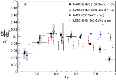
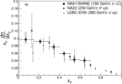
Figure 14: Scaled $x_{\text{F}}$-spectra of meson production in $\pi^{-}$+C production interactions at 158 and $350\,\mbox{Ge\kern-1.00006ptV}\kern-1.00006pt/\kern-0.50003ptc$ ($350\,\mbox{Ge\kern-1.00006ptV}\kern-1.00006pt/\kern-0.50003ptc$ shifted by 0.035). The error bars show the statistical, the bands indicate systematic uncertainties (where available). The black points are from this experiment, blue squares are from NA22 [17], red triangles are from LEBC-EHS (NA27) [60]. $\rho^{0}$ spectra are shown on the left and $\omega$ spectra on the right.

5 Summary

This article presents experimental results on $\rho^{0}$, $\omega$ and K^∗0 $x_{\text{F}}$-spectra in $\pi^{-}$+C production interactions at $158\,\mbox{Ge\kern-1.00006ptV}\kern-1.00006pt/\kern-0.50003ptc$ and the $\rho^{0}$ spectra at 350 $\mbox{Ge\kern-1.00006ptV}\kern-1.00006pt/\kern-0.50003ptc$ from the spectrometer at the CERN SPS. These results are the first $\pi^{-}$+C measurements taken in this energy range and are important to tune hadronic interaction models used to understand the measurements of cosmic-ray air showers.

The comparisons of the measured spectra to predictions of hadronic interaction models suggests that for all models further tuning is required to reproduce the measured spectra of $\rho^{0}$, $\omega$ and K^∗0 mesons in the full range of $x_{\text{F}}$. Recent re-tunes of these models to resonance data in $\pi+p$ interactions resulted in changes of the muon number at ground of up to 25% [14, 59]. The new data provided here for $\pi$+C interactions gives a more adequate reference for pion-air interactions relevant for air showers and will help to establish the effect of forward resonance production on muons in air showers with the precision needed for using the muon number to estimate the particle type of primary cosmic rays, as e.g. planned within the upgrade of the Pierre Auger Observatory [62].

Appendix A Tables of measured resonance yields

Table 4: Average multiplicity of $\rho^{0}$ in $\pi^{-}$+C interactions at 158 $\mbox{Ge\kern-1.00006ptV}\kern-1.00006pt/\kern-0.50003ptc$ and 350 $\mbox{Ge\kern-1.00006ptV}\kern-1.00006pt/\kern-0.50003ptc$, binned in $x_{\text{F}}$.

$p_{\text{beam}}/(\mbox{Ge\kern-1.00006ptV}\kern-1.00006pt/\kern-0.50003ptc)$	$x_{\text{F}}$						$\langle{x_{\text{F}}}\rangle$		$\mathrm{d}n/\mathrm{d}x_{\text{F}}$		$\Delta_{\text{stat}}$		$\Delta_{\text{sys}}^{+}$		$\Delta_{\text{sys}}^{-}$
158	0.	0	–		0.	15	0.	071	0.	737	0.	040	0.	194	0.	232
	0.	15	–		0.	3	0.	212	0.	394	0.	016	0.	011	0.	035
	0.	3	–		0.	4	0.	343	0.	314	0.	015	0.	015	0.	036
	0.	4	–		0.	5	0.	443	0.	236	0.	009	0.	016	0.	016
	0.	5	–		0.	6	0.	542	0.	184	0.	007	0.	012	0.	011
	0.	6	–		0.	7	0.	641	0.	153	0.	006	0.	006	0.	006
	0.	7	–		0.	8	0.	741	0.	106	0.	005	0.	005	0.	005
	0.	8	–		0.	9	0.	841	0.	076	0.	004	0.	012	0.	012
	0.	9	–		1.	0	0.	939	0.	038	0.	004	0.	010	0.	010
350	0.	0	–		0.	15	0.	062	0.	790	0.	0419	0.	166	0.	274
	0.	15	–		0.	3	0.	199	0.	499	0.	0202	0.	033	0.	097
	0.	3	–		0.	4	0.	333	0.	343	0.	0246	0.	066	0.	017
	0.	4	–		0.	5	0.	431	0.	230	0.	0235	0.	093	0.	045

Table 5: Average multiplicity of $\omega$ in $\pi^{-}$+C interactions at 158 $\mbox{Ge\kern-1.00006ptV}\kern-1.00006pt/\kern-0.50003ptc$, binned in $x_{\text{F}}$.

$p_{\text{beam}}/(\mbox{Ge\kern-1.00006ptV}\kern-1.00006pt/\kern-0.50003ptc)$	$x_{\text{F}}$						$\langle{x_{\text{F}}}\rangle$		$\mathrm{d}n/\mathrm{d}x_{\text{F}}$		$\Delta_{\text{stat}}$		$\Delta_{\text{sys}}^{+}$		$\Delta_{\text{sys}}^{-}$
158	0.	0	–		0.	15	0.	071	1.	360	0.	082	0.	295	0.	156
	0.	15	–		0.	3	0.	212	0.	432	0.	028	0.	025	0.	032
	0.	3	–		0.	4	0.	343	0.	224	0.	026	0.	015	0.	020
	0.	4	–		0.	5	0.	443	0.	133	0.	015	0.	005	0.	010
	0.	5	–		0.	6	0.	542	0.	078	0.	016	0.	015	0.	012
	0.	6	–		0.	7	0.	641	0.	063	0.	018	0.	011	0.	009

Table 6: Average multiplicity of K^∗0 in $\pi^{-}$+C interactions at 158 $\mbox{Ge\kern-1.00006ptV}\kern-1.00006pt/\kern-0.50003ptc$, binned in $x_{\text{F}}$.

$p_{\text{beam}}/(\mbox{Ge\kern-1.00006ptV}\kern-1.00006pt/\kern-0.50003ptc)$	$x_{\text{F}}$						$\langle{x_{\text{F}}}\rangle$		$\mathrm{d}n/\mathrm{d}x_{\text{F}}$		$\Delta_{\text{stat}}$		$\Delta_{\text{sys}}^{+}$		$\Delta_{\text{sys}}^{-}$
158	0.	0	–		0.	15	0.	071	1.	073	0.	061	0.	468	0.	131
	0.	15	–		0.	3	0.	212	0.	417	0.	022	0.	149	0.	013
	0.	3	–		0.	4	0.	343	0.	176	0.	016	0.	025	0.	015
	0.	4	–		0.	5	0.	443	0.	101	0.	010	0.	009	0.	011
	0.	5	–		0.	6	0.	542	0.	054	0.	007	0.	008	0.	008
	0.	6	–		0.	7	0.	641	0.	030	0.	006	0.	004	0.	004
	0.	7	–		0.	8	0.	741	0.	013	0.	004	0.	001	0.	002
	0.	8	–		0.	9	0.	841	0.	016	0.	003	0.	004	0.	005

Appendix B Examples of templates of resonances and background

(a) charge mixing

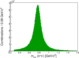
(b) $\rho^{0}$

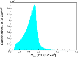
(c) K^∗0

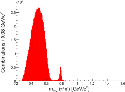
(d) $\omega$

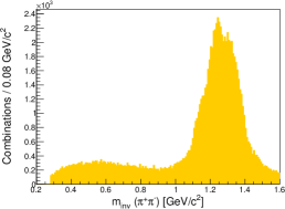
(e) f₂

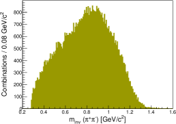
(f) a₂

(g) f₀

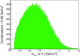
(h) $\rho^{3}$

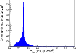
(i) K${}^{0}_{\text{S}}$

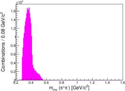
(j) $\eta$

Figure 15: Templates of the invariant mass spectra of resonances and background at 158 $\mbox{Ge\kern-1.00006ptV}\kern-1.00006pt/\kern-0.50003ptc$ in the range $0.4<x_{\text{F}}<0.5$ assuming pion masses.

Appendix C Results of template fits

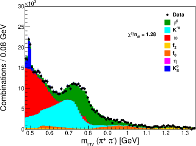
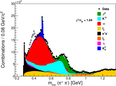
(a) $0<x_{\text{F}}<0.15$

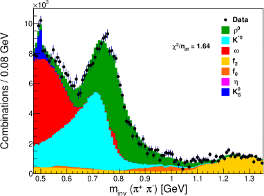
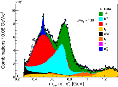
(b) $0.15<x_{\text{F}}<0.3$

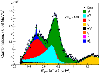
(c) $0.3<x_{\text{F}}<0.4$

Figure 16: Invariant mass distribution of opposite charged particles, calculated assuming pion masses, in $\pi^{-}$+C interactions at 158 $\mbox{Ge\kern-1.00006ptV}\kern-1.00006pt/\kern-0.50003ptc$. Dots with error bars denote the data and the fitted resonance templates are shown as filled histograms. The fitted background and high mass resonances have been subtracted. Two fits with different $m_{\text{inv}}(\pi^{+}\pi^{-})$ ranges are shown on the left and right column. The fit range is equal to the displayed range, but in the extended-range fit on the right the mass region $0.35<m_{\text{inv}}(\pi^{+}\pi^{-})<0.4$ is excluded (see discussion App. D), as indicated by the grey points.

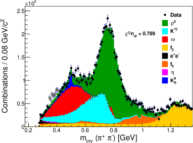
(a) $0.4<x_{\text{F}}<0.5$

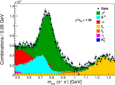
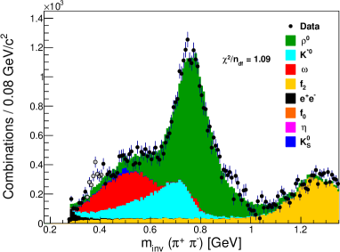
(b) $0.5<x_{\text{F}}<0.6$

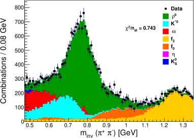
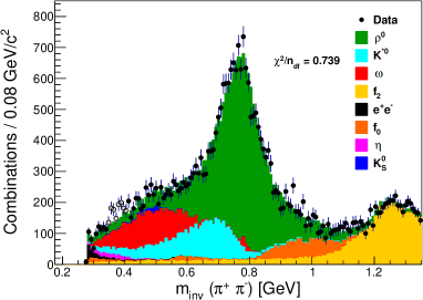
(c) $0.6<x_{\text{F}}<0.7$

Figure 17: Invariant mass distribution of opposite charged particles, calculated assuming pion masses, in $\pi^{-}$+C interactions at 158 $\mbox{Ge\kern-1.00006ptV}\kern-1.00006pt/\kern-0.50003ptc$. Dots with error bars denote the data and the fitted resonance templates are shown as filled histograms. The fitted background and high mass resonances have been subtracted. Two fits with different $m_{\text{inv}}(\pi^{+}\pi^{-})$ ranges are shown on the left and right column. The fit range is equal to the displayed range, but in the extended-range fit on the right the mass region $0.35<m_{\text{inv}}(\pi^{+}\pi^{-})<0.4$ is excluded (see discussion App. D), as indicated by the grey points.

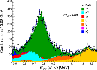
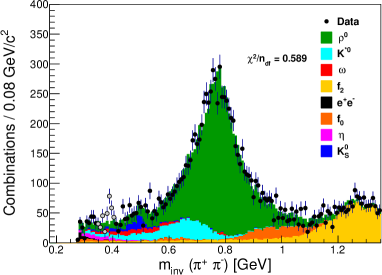
(a) $0.7<x_{\text{F}}<0.8$

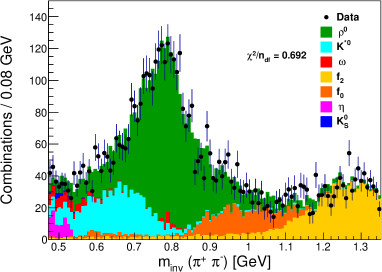
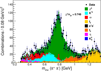
(b) $0.8<x_{\text{F}}<0.9$

(c) $0.9<x_{\text{F}}<1$

Figure 18: Invariant mass distribution of opposite charged particles, calculated assuming pion masses, in $\pi^{-}$+C interactions at 158 $\mbox{Ge\kern-1.00006ptV}\kern-1.00006pt/\kern-0.50003ptc$. Dots with error bars denote the data and the fitted resonance templates are shown as filled histograms. The fitted background and high mass resonances have been subtracted. Two fits with different $m_{\text{inv}}(\pi^{+}\pi^{-})$ ranges are shown on the left and right column. The fit range is equal to the displayed range, but in the extended-range fit on the right the mass region $0.35<m_{\text{inv}}(\pi^{+}\pi^{-})<0.4$ is excluded (see discussion App. D), as indicated by the grey points.

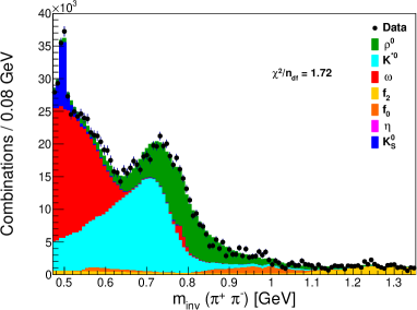
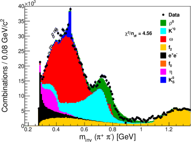
(a) $0<x_{\text{F}}<0.15$

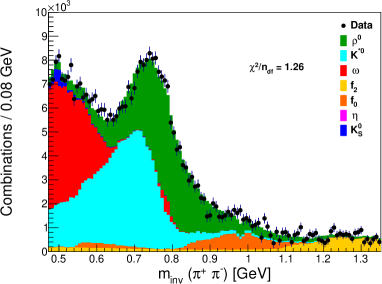
(b) $0.15<x_{\text{F}}<0.3$

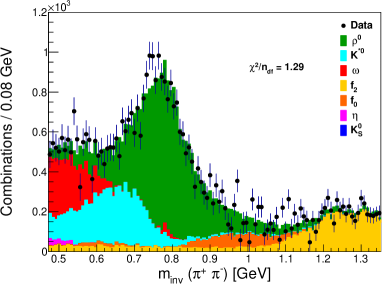
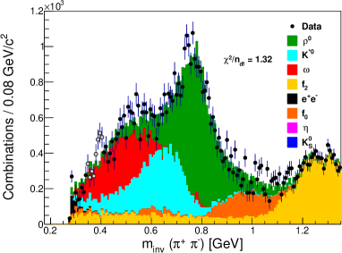
(c) $0.3<x_{\text{F}}<0.4$

Figure 19: Invariant mass distribution of opposite charged particles, calculated assuming pion masses, in $\pi^{-}$+C interactions at 350 $\mbox{Ge\kern-1.00006ptV}\kern-1.00006pt/\kern-0.50003ptc$. Dots with error bars denote the data and the fitted resonance templates are shown as filled histograms. The fitted background and high mass resonances have been subtracted. Two fits with different $m_{\text{inv}}(\pi^{+}\pi^{-})$ ranges are shown on the left and right column. The fit range is equal to the displayed range, but in the extended-range fit on the right the mass region $0.35<m_{\text{inv}}(\pi^{+}\pi^{-})<0.4$ is excluded (see discussion App. D), as indicated by the grey points.

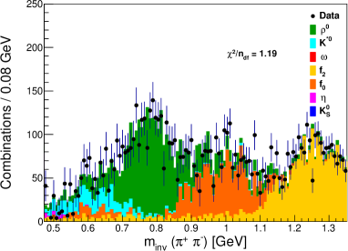
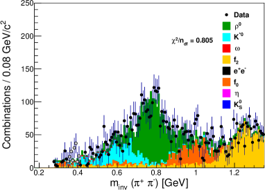
(a) $0.4<x_{\text{F}}<0.5$

Figure 20: Invariant mass distribution of opposite charged particles, calculated assuming pion masses, in $\pi^{-}$+C interactions at 350 $\mbox{Ge\kern-1.00006ptV}\kern-1.00006pt/\kern-0.50003ptc$. Dots with error bars denote the data and the fitted resonance templates are shown as filled histograms. The fitted background and high mass resonances have been subtracted. The fit range is equal to the displayed range, but in the extended-range fit on the right the mass region $0.35<m_{\text{inv}}(\pi^{+}\pi^{-})<0.4$ is excluded (see discussion App. D), as indicated by the grey points.

Appendix D Discussion of the bump in the extended range fit

The fits with the extended invariant mass range show a bump in the data at low $x_{\text{F}}$ that is not described by the template fit (see right columns in Figs. 16 to 20). A large number of templates from different resonances were investigated to describe the excess of combinations at low invariant masses. The resonances were chosen from the particles with the highest yield in the region of invariant mass where the excess was located. Most of these resonances have a dominant decay which is either into three (or more) particles, or two-body decays but into particles other than two pions. As the invariant mass in this analysis is calculated assuming the particles are pions from a two-body decay, this will shift the calculated mass away from the true mass of the resonance. The studied resonances are listed in the table below and they were chosen by looking at the invariant mass distribution of particles produced in Epos 1.99 that produce a combination of negative and positive tracks in the region of $m_{\text{inv}}(\pi^{+}\pi^{-})\approx 0.375\,\mbox{Ge\kern-1.00006ptV}\kern-1.00006pt/\kern-0.50003ptc^{2}$. Particles not produced by this model were not considered.

resonance	mass / $(\mbox{Ge\kern-0.90005ptV}\kern-0.90005pt/\kern-0.45003ptc^{2})$	${\approx}$peak in $m_{\text{inv}}(\pi^{+}\pi^{-})/(\mbox{Ge\kern-0.90005ptV}\kern-0.90005pt/\kern-0.45003ptc^{2})$	dominant decay
$\phi$	1.020	0.37	K+K-
$\Lambda$	1.115	0.34	p $\pi^{-}$
$\Delta$	1.230	0.58	N $\pi\,\pi$
$N(1440)$	1.440	0.43	N $\pi\,\pi$
$a_{2}^{\pm}$	1.320	0.46	3$\pi$
$\rho_{3}^{\pm}$	1.690	0.50	4$\pi$, 2$\pi$
$\eta^{{}^{\prime}}$	0.958	0.35	$\pi^{+}\pi^{-}\eta$
$f_{2}^{{}^{\prime}}$	1.525	1.15	K $\bar{\text{K}}$
$f_{0}(1500)$	1.500	0.45	2$\pi$, 4$\pi$
$f_{1}$	1.285	0.41	4$\pi$, $\eta\,2\pi$
$f_{1}(1420)$	1.420	0.42	K $\bar{\text{K}}$ $\pi$
K${}_{L}^{0}$	0.497	0.39	$\pi^{+}\pi^{-}\pi^{0}$
K	0.494	0.44	$\pi^{+}\pi^{+}\pi^{-}$

We found that none of these resonances can describe the bump seen at a $m_{\text{inv}}(\pi^{+}\pi^{-})\approx 0.375\,\mbox{Ge\kern-1.00006ptV}\kern-1.00006pt/\kern-0.50003ptc^{2}$. The best-fit particles are the first two in the table: $\phi$ and $\Lambda$. However both of these have features that are not present in the data. $\phi$ has a peak in $m_{\text{inv}}(\pi^{+}\pi^{-})$ just below the bump and the $\Lambda$-template is too broad with no peak near the bump. All other templates were either too broad, had no peak, or their peak was too far away from the bump. The conversion of $\gamma$ into $e^{+}e^{-}$ was also investigated, but the corresponding templates also can not describe the bump. Furthermore, we tried combinations of the resonances listed above without success, though we can not exclude that a particular combination could fit the bump since not all possible combinations were explored.

From a study of the ionisation energy deposit of the tracks in the TPCs we conclude that the bump is caused by pion combinations. The bump is not caused by re-interactions in the detector or the decay of long lived particles as it remains present even under the tightening of impact parameter cuts, which would remove such particles. It is interesting to note that the mass of the bump compatible with the f₀ (500) meson, however the width seen here is much smaller than quoted by the particle data group [51].

Appendix E Yield ratios

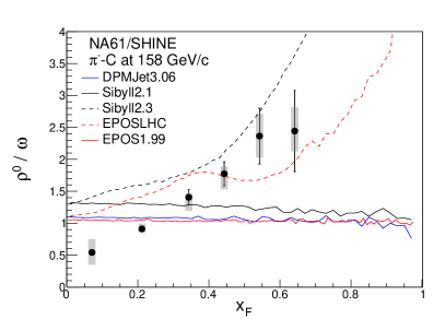
(a) $\rho^{0}$/$\omega$

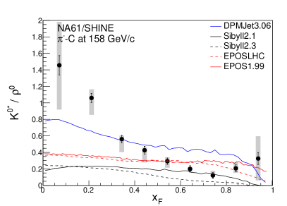
(b) K^∗0 and $\rho^{0}$

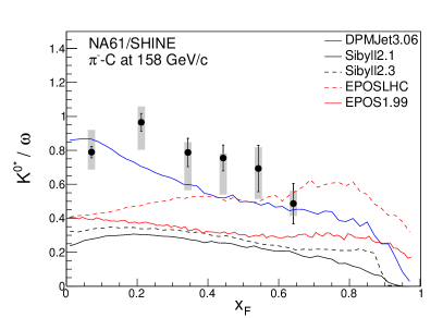
(c) K^∗0/$\omega$

Figure 21: Ratio of meson spectra in $\pi^{-}$+C production interactions at $158\,\mbox{Ge\kern-1.00006ptV}\kern-1.00006pt/\kern-0.50003ptc$. The dots with error bars show the data and its statistical uncertainties. The shaded boxes denote the systematic uncertainties. The lines depict predictions of hadronic interaction models: red – Epos 1.99, blue – DPMJet 3.06, black – Sibyll 2.1, dashed red – Epos LHC, dashed black – Sibyll 2.3.

.

The Collaboration

A. Aduszkiewicz¹⁶, Y. Ali¹³, E.V. Andronov²², T. Antićić³, B. Baatar²⁰, M. Baszczyk¹⁴, S. Bhosale¹¹, A. Blondel²⁵, M. Bogomilov², A. Brandin²¹, A. Bravar²⁵, J. Brzychczyk¹³, S.A. Bunyatov²⁰, O. Busygina¹⁹, H. Cherif⁷, M. Ćirković²³, T. Czopowicz¹⁸, A. Damyanova²⁵, N. Davis¹¹, H. Dembinski⁵, M. Deveaux⁷, W. Dominik¹⁶, P. Dorosz¹⁴, J. Dumarchez⁴, R. Engel⁵, A. Ereditato²⁴, S. Faas⁵, G.A. Feofilov²², Z. Fodor^8,17, C. Francois²⁴, A. Garibov¹, X. Garrido⁵, M. Gaździcki^7,10, M. Golubeva¹⁹, K. Grebieszkow¹⁸, F. Guber¹⁹, A. Haesler²⁵, A.E. Hervé⁵, J. Hylen²⁶, S.N. Igolkin²², A. Ivashkin¹⁹, S.R. Johnson²⁸, K. Kadija³, E. Kaptur¹⁵, M. Kiełbowicz¹¹, V.A. Kireyeu²⁰, V. Klochkov⁷, V.I. Kolesnikov²⁰, D. Kolev², A. Korzenev²⁵, V.N. Kovalenko²², K. Kowalik¹², S. Kowalski¹⁵, M. Koziel⁷, A. Krasnoperov²⁰, W. Kucewicz¹⁴, M. Kuich¹⁶, A. Kurepin¹⁹, D. Larsen¹³, A. László⁸, T.V. Lazareva²², M. Lewicki¹⁷, B. Lundberg²⁶, B. Łysakowski¹⁵, V.V. Lyubushkin²⁰, M. Maćkowiak-Pawłowska¹⁸, B. Maksiak¹⁸, A.I. Malakhov²⁰, D. Manić²³, A. Marchionni²⁶, A. Marcinek¹¹, A.D. Marino²⁸, I.C. Mariş⁵, K. Marton⁸, H.-J. Mathes⁵, T. Matulewicz¹⁶, V. Matveev²⁰, G.L. Melkumov²⁰, A.O. Merzlaya²², B. Messerly²⁹, Ł. Mik¹⁴, G.B. Mills²⁷, S. Morozov^19,21, S. Mrówczyński¹⁰, Y. Nagai²⁸, M. Naskręt¹⁷, V. Ozvenchuk¹¹, V. Paolone²⁹, M. Pavin^4,3, O. Petukhov^19,21, C. Pistillo²⁴, R. Płaneta¹³, P. Podlaski¹⁶, B.A. Popov^20,4, M. Posiadała¹⁶, S. Puławski¹⁵, J. Puzović²³, R. Rameika²⁶, W. Rauch⁶, M. Ravonel²⁵, R. Renfordt⁷, E. Richter-Wąs¹³, D. Röhrich⁹, E. Rondio¹², M. Roth⁵, M. Ruprecht⁵, B.T. Rumberger²⁸, A. Rustamov^1,7, M. Rybczynski¹⁰, A. Rybicki¹¹, A. Sadovsky¹⁹, K. Schmidt¹⁵, I. Selyuzhenkov²¹, A.Yu. Seryakov²², P. Seyboth¹⁰, M. Słodkowski¹⁸, A. Snoch⁷, P. Staszel¹³, G. Stefanek¹⁰, J. Stepaniak¹², M. Strikhanov²¹, H. Ströbele⁷, T. Šuša³, M. Szuba⁵, A. Taranenko²¹, A. Tefelska¹⁸, D. Tefelski¹⁸, V. Tereshchenko²⁰, A. Toia⁷, R. Tsenov², L. Turko¹⁷, R. Ulrich⁵, M. Unger⁵, F.F. Valiev²², D. Veberič⁵, V.V. Vechernin²², M. Walewski¹⁶, A. Wickremasinghe²⁹, C. Wilkinson²⁴, Z. Włodarczyk¹⁰, A. Wojtaszek-Szwarc¹⁰, O. Wyszyński¹³, L. Zambelli^4,1, E.D. Zimmerman²⁸, and R. Zwaska²⁶

¹National Nuclear Research Center, Baku, Azerbaijan
²Faculty of Physics, University of Sofia, Sofia, Bulgaria
³Ruđer Bošković Institute, Zagreb, Croatia
⁴LPNHE, University of Paris VI and VII, Paris, France
⁵Karlsruhe Institute of Technology, Karlsruhe, Germany
⁶Fachhochschule Frankfurt, Frankfurt, Germany
⁷University of Frankfurt, Frankfurt, Germany
⁸Wigner Research Centre for Physics of the Hungarian Academy of Sciences, Budapest, Hungary
⁹University of Bergen, Bergen, Norway
¹⁰Jan Kochanowski University in Kielce, Poland
¹¹H. Niewodniczański Institute of Nuclear Physics of the Polish Academy of Sciences, Kraków, Poland
¹²National Centre for Nuclear Research, Warsaw, Poland
¹³Jagiellonian University, Cracow, Poland
¹⁴University of Science and Technology, Cracow, Poland
¹⁵University of Silesia, Katowice, Poland
¹⁶University of Warsaw, Warsaw, Poland
¹⁷University of Wrocław, Wrocław, Poland
¹⁸Warsaw University of Technology, Warsaw, Poland
¹⁹Institute for Nuclear Research, Moscow, Russia
²⁰Joint Institute for Nuclear Research, Dubna, Russia
²¹National Research Nuclear University (Moscow Engineering Physics Institute), Moscow, Russia
²²St. Petersburg State University, St. Petersburg, Russia
²³University of Belgrade, Belgrade, Serbia
²⁴University of Bern, Bern, Switzerland
²⁵University of Geneva, Geneva, Switzerland
²⁶Fermilab, Batavia, USA
²⁷Los Alamos National Laboratory, Los Alamos, USA
²⁸University of Colorado, Boulder, USA
²⁹University of Pittsburgh, Pittsburgh, USA

References

- [1] R. Engel, D. Heck, and T. Pierog Ann. Rev. Nucl. Part. Sci. 61 (2011) 467–489.
- [2] J. Abraham et al., [Pierre Auger Collab.] Nucl. Instrum. Meth. A523 (2004) 50–95.
- [3] R. Abbasi et al., [IceCube Collab.] Nucl. Instrum. Meth. A700 (2013) 188–220.
- [4] G. Navarra et al., [KASCADE-Grande Collab.] Nucl. Instrum. Meth. A518 (2004) 207–209.
- [5] T. Abu-Zayyad et al., [Telescope Array Collab.] Nucl. Instrum. Meth. A689 (2012) 87–97.
- [6] T. Abu-Zayyad et al. Phys. Rev. Lett. 84 (2000) 4276–4279.
- [7] J. C. Arteaga-Velazquez et al. EPJ Web Conf. 52 (2013) 07002.
- [8] A. Aab et al., [Pierre Auger Collab.] Phys. Rev. D91 (2015) 032003.
- [9] A. Aab et al., [Pierre Auger Collab.] Phys. Rev. D90 (2014) 012012.
- [10] A. Aab et al., [Pierre Auger Collab.] Phys. Rev. Lett. 117 no. 19, (2016) 192001.
- [11] J. Matthews Astropart. Phys. 22 (2005) 387–397.
- [12] T. Pierog and K. Werner Phys. Rev. Lett. 101 (2008) 171101.
- [13] H.-J. Drescher Phys. Rev. D77 (2008) 056003.
- [14] S. Ostapchenko EPJ Web Conf. 52 (2013) 02001.
- [15] M. Adamus et al., [NA22 Collab.] Z. Phys. C35 (1987) 7. [Sov. J. Nucl. Phys.47,271(1988)].
- [16] I. V. Azhinenko et al., [EHS/NA22 Collab.] Z. Phys. C46 (1990) 525–536.
- [17] N. Agababyan et al., [EHS-NA22 Collab.] Z. Phys. C46 (1990) 387–395.
- [18] H.-J. Drescher and G. R. Farrar Astropart. Phys. 19 (2003) 235 – 244.
- [19] I. Mariş, [NA61/SHINE Collab.] Proc. 31st ICRC (2009) 1059.
- [20] T. Eichten et al. Nucl. Phys. B44 (1972) 333 – 343.
- [21] T. Abbott et al., [E-802 Collab.] Phys. Rev. D45 (1992) 3906–3920.
- [22] G. Ambrosini et al., [SPY Collab.] Phys. Lett. B425 (1998) 208 – 214.
- [23] C. Alt et al. Eur. Phys. J. C49 (2007) 897–917.
- [24] M. Apollonio et al., [HARP Collab.] Phys. Rev. C80 (2009) 035208.
- [25] M. Catanesi et al., [HARP Collab.] Astropart. Phys. 29 (2008) 257 – 281.
- [26] M. Catanesi et al., [HARP Collab.] Astropart. Phys. 30 (2008) 124 – 132.
- [27] D. S. Barton et al. Phys. Rev. D27 (1983) 2580.
- [28] M. Aguilar-Benitez et al., [LEBC-EHS Collab.] Z. Phys. C44 (1989) 531.
- [29] J. E. Elias et al. Phys. Rev. D22 (1980) 13–35.
- [30] N. Abgrall et al., [NA61/SHINE Collab.] JINST 9 (2014) P06005.
- [31] M. Unger, [NA61/SHINE Collab.] EPJ Web Conf. 52 (2013) 01009.
- [32] H. Dembinski, [NA61/SHINE Collab.] Proc. 33rd ICRC (2013) 0688.
- [33] A. Herve, [NA61/SHINE Collab.] PoS ICRC2015 (2015) 330, arXiv:1509.06586.
- [34] A. E. Kiryunin et al. Nucl. Instrum. Meth. A560 (2006) 278–290.
- [35] J. V. Damgov, [CMS HCAL Collab.] AIP Conf. Proc. 867 (2006) 471–478. [,471(2006)].
- [36] C. Adloff et al., [CALICE Collab.] JINST 8 (2013) 07005.
- [37] S. Afanasev et al., [NA49 Collab.] Nucl.Instrum.Meth. A430 (1999) 210–244.
- [38] C. Bovet, S. Milner, and A. Placci IEEE Trans. Nucl. Sci. 25 (1978) 572–576.
- [39] N. Abgrall, [NA61/SHINE Collab.]. http://cds.cern.ch/record/1113279.
- [40] S. Roesler, R. Engel, and J. Ranft, The Monte Carlo Event Generator DPMJET-III, pp. 1033–1038. Springer Berlin Heidelberg, 2001.
- [41] T. Pierog, private communication (2013).
- [42] R. Brun et al., GEANT: Detector Description and Simulation Tool. CERN, 1993. Long Writeup W5013.
- [43] N. Abgrall et al., [NA61/SHINE Collab.] Phys. Rev. C84 (2011) 034604.
- [44] G. Jancso et al. Nucl. Phys. B124 (1977) 1–11.
- [45] M. K. Köhler et al., [ALICE Collab.] Nucl. Phys. A931 (2014) 665–669.
- [46] ATLAS Collaboration ATLAS-CONF-2012-030 (2012) .
- [47] A. Abulencia et al., [CDF Collab.] Phys. Rev. D73 (2006) 032003.
- [48] S. Chatrchyan et al., [CMS Collab.] Eur. Phys. J. C 72 (2012) 2202.
- [49] T. Pierog, C. Baus, and R. Ulrich. https://web.ikp.kit.edu/rulrich/crmc.html.
- [50] T. Pierog et al. Phys. Rev. C92 (2015) 034906.
- [51] C. Patrignani et al., [Particle Data Group Collab.] Chin. Phys. C40 no. 10, (2016) 100001.
- [52] R. S. Hayano and T. Hatsuda Rev. Mod. Phys. 82 (2010) 2949.
- [53] X.-M. Jin and D. B. Leinweber Phys. Rev. C52 (1995) 3344–3352.
- [54] C. Adler et al., [STAR Collab.] Phys. Rev. Lett. 89 (2002) 272302.
- [55] S. Teis et al. Z. Phys. A356 (1997) 421–435.
- [56] J. H. Koch, N. Ohtsuka, and E. J. Moniz Annals Phys. 154 (1984) 99–160.
- [57] S. Ostapchenko Phys. Rev. D83 (2011) 014018.
- [58] E.-J. Ahn et al. Phys. Rev. D80 (2009) 094003.
- [59] F. Riehn et al. PoS (ICRC2015) (2015) 558, arXiv:1510.00568.
- [60] M. Aguilar-Benitez et al., [LEBC-EHS Collab.] Z. Phys. C44 (1989) 531–539.
- [61] M. Adamus et al., [NA22 Collab.] Z. Phys. C32 (1986) 475.
- [62] A. Aab et al., [Pierre Auger Collab.] arXiv:1604.03637 [astro-ph.IM].