Extracting Lyapunov exponents from the echo dynamics of Bose-Einstein condensates on a lattice

Abstract

We propose theoretically an experimentally realizable method to demonstrate the Lyapunov instability and to extract the value of the largest Lyapunov exponent for a chaotic many-particle interacting system. The proposal focuses specifically on a lattice of coupled Bose-Einstein condensates in the classical regime describable by the discrete Gross-Pitaevskii equation. We suggest to use imperfect time-reversal of system’s dynamics known as Loschmidt echo, which can be realized experimentally by reversing the sign of the Hamiltonian of the system. The routine involves tracking and then subtracting the noise of virtually any observable quantity before and after the time-reversal. We support the theoretical analysis by direct numerical simulations demonstrating that the largest Lyapunov exponent can indeed be extracted from the Loschmidt echo routine. We also discuss possible values of experimental parameters required for implementing this proposal.

I Introduction

Historically, statistical physics was established by Boltzmann, Gibbs and others on the basis of the assumption that the internal dynamics of a typical interacting many-body system is chaotic. Yet one of the outstanding issues of the foundations of modern statistical physics remains to produce experimental evidence that a typical many-particle system is indeed chaotic. A classical system is called chaotic if it has at least one positive Lyapunov exponent, which characterizes exponential sensitivity of phase space trajectories to infinitesimally small perturbations of initial conditions. The practical challenge here is that it is impossible: first, to monitor all phase space coordinates of a many-body system and, second, to prepare initial conditions with very high accuracy required for extracting Lyapunov exponents. On top of this, microscopic many-particle systems are not classical, but quantum, which makes the whole notion of phase space not very well defined. To make progress on the issue of chaos in statistical physics, it is reasonable to separate the difficulty of extracting Lyapunov exponents for classical systems from the difficulty of defining quantum chaos Haake (2013) as such. In this paper, we concentrate on the former.

A method of extracting the largest Lyapunov exponent of a many-particle classical system without using full phase space trajectories was proposed recently in Ref. Fine et al. (2014). The method is based on tracking the initial behavior of virtually any observable quantity in response to imperfect reversal of system’s dynamics. This imperfect reversal is called Loschmidt echo. It can be realized experimentally by reversing the sign of the Hamiltonian of a system.

In Ref. Fine et al. (2014) the possibility to extract the largest Lyapunov exponent was demonstrated for a lattice of classical spins, whereas in the present article we generalize the same analysis to a system of coupled Bose-Einstein condensates (BEC) on a lattice in the regime describable by the classical discrete Gross-Pitaevskii equation (DGPE) Gross (1961); Pitaevskii (1961). In other words, we consider the classical dynamics of this system, despite the fact that the system is of quantum origin. The advantage of coupled Bose-Einstein condensates over classical spins is that the former were already realized experimentally. In particular, Struck et al. Struck et al. (2011) have recently performed an experimental simulation of frustrated classical magnetism using Bose-Einstein condensates of ultracold atoms. However, Ref. Struck et al. (2011) concentrated on simulating low-temperature equilibrium properties of the system, while the present article concentrates on finite-temperature dynamics and its time-reversal. Time-reversal of DGPE was previously considered in Refs. Weiss (2012, 2013), but not in the context of extracting the largest Lyapunov exponent. An alternative time-reversal procedure analogous to the sign change of all particle velocities in classical mechanics was already experimentally realized for the propagation of a wave-packet of intense light in a nonlinear crystal, which is describable by the continuous nonlinear Schrödinger equation, an analog of the continuous Gross-Pitaevskii equation Sun et al. (2012).

The structure of the present paper is as follows. In Section II, we describe the general idea how one extracts the largest Lyapunov exponent from Loschmidt echo in a many-particle system. Then, in Section III we formally define the problem of Loschmidt echo for interacting BECs on a lattice. In Section IV, we provide some details of the numerical algorithm and describe the methods of extracting the largest Lyapunov exponent of the system governed by DGPE in one, two and three dimensions: the direct one and from the Loschmidt echo. In Section V, we consider the limits of applicability of DGPE imposing constraints on experimental realization. Finally, in Section VI, we make a proposal of an experimental setting that could potentially verify our theoretical results. In particular, we describe the possible range of system parameters where the approximations we used are valid.

II Lyapunov exponent from Loschmidt echo: general idea

In general, a conservative system with $2N$-dimensional phase space is characterized by a spectrum of $N$ pairs of Lyapunov exponents of the same absolute value and opposite signs. When two phase space trajectories $\mathbf{R}_{1}(t)$ and $\mathbf{R}_{2}(t)$ are initially infinitesimally close to each other, their separation from each other after sufficiently long time is controlled by the largest positive Lyapunov exponent $\lambda_{\max}$ of the system. $\lambda_{\max}$ describes the average expansion rate along the direction of the corresponding eigenvector in tangential space, which typically has fluctuating projections on all phase space axes. Let us choose one of the axes of the phase space to correspond to the observable quantity of interest. In such a case, it is expected that the projection of the difference between the two separating phase trajectories $\mathbf{R}_{1}(t)$ and $\mathbf{R}_{2}(t)$ on this axis will exhibit erratic behavior, but the envelope of that behavior will grow exponentially and will be controlled by $\lambda_{\max}$. If the system is ergodic the value of $\lambda_{\max}$ does not depend on where the two phase space trajectories start, but the corresponding eigenvector and the resulting fluctuating projection on the chosen axis do. It is therefore expected that if one averages over an ensemble of initial conditions on the same energy shell, then the fluctuating component of the difference between the trajectories would average into a constant multiplied by a factor $\exp\left(\lambda_{\max}t\right)$.

As suggested in Ref. Fine et al. (2014), the above considerations can be converted into the following scheme of extracting $\lambda_{\max}$. Let us consider equilibrium noise of observable $X$ as a function of time $t$ for a system governed by Hamiltonian ${\cal H}$. Next, we record this noise during time-interval from $0$ to $\tau$ and at time $\tau$ reverse the sign of the Hamiltonian with a slight perturbation of the system at the moment of Hamiltonian reversal. If the perturbation is infinitesimally small, the quantity $X(\tau+\Delta t)$ will be tracking the quantity $X(\tau-\Delta t)$, while gradually departing from it as the echo time $\Delta t$ increases. After sufficiently long time, $\left|X(\tau+\Delta t)-X(\tau-\Delta t)\right|$ should be modulated by $\exp\left(\lambda_{\max}\Delta t\right)$. The preceding consideration then suggests that $\lambda_{\max}$ can be extracted from the following average over the initial conditions

$$\lambda_{\max}=\frac{1}{\Delta t}\left\langle\log\left|X(\tau+\Delta t)-X(\tau-\Delta t)\right|\right\rangle,$$ (1)

where $\tau$ should be larger than $\Delta t$ .

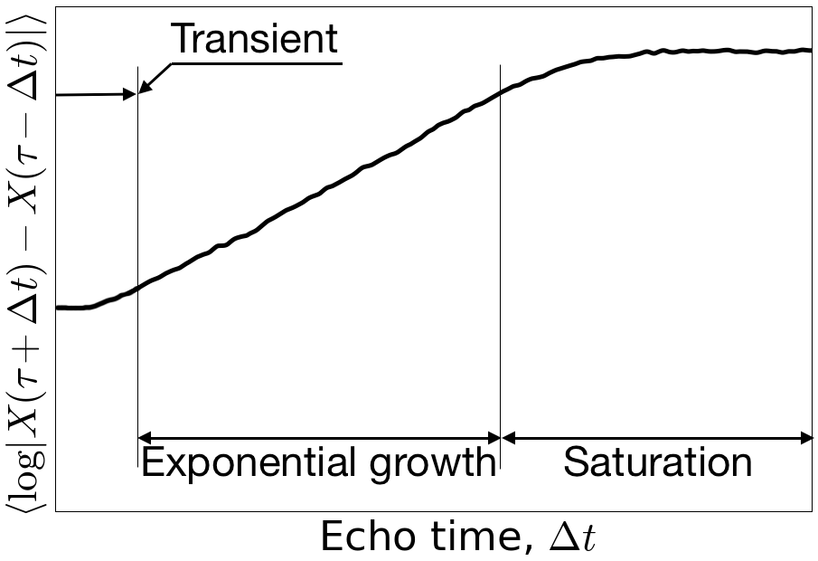
Figure 1: Sketch of a typical Loschmidt echo response $\left\langle\log\left|X(\tau+\Delta t)-X(\tau-\Delta t)\right|\right\rangle$ (thick black line). Three characteristic regimes described in the text are indicated: transient, exponential growth and saturation.

Typical behavior of $\left\langle\log\left|X(\tau+\Delta t)-X(\tau-\Delta t)\right|\right\rangle$ as a function of $\Delta t$ for almost any reasonable quantity $X$ is qualitatively depicted in Fig. 1. It starts growing from a tiny value at $\Delta t=0$ and then evolves through a transient regime, where all Lyapunov exponents contribute to the growth, and the largest one is not dominant yet. After that, it enters the exponential growth regime, where the largest Lyapunov exponent controls the growth. For any finite initial difference between the two departing phase space trajectories, the exponential growth regime is eventually followed by the saturation regime, where $\left|X(\tau+\Delta t)-X(\tau-\Delta t)\right|$ is no longer small enough to be describable by linearized dynamics. This means that, experimentally or numerically, the perturbation of a perfect time-reversal should be small enough, so that the time $\Delta t$ for which $\left|X(\tau+\Delta t)-X(\tau-\Delta t)\right|$ remains small is sufficiently long to extract $\lambda_{\max}$.

As follows from the above analysis, the method does not use any specific properties of quantity $X$, thus it can be either scalar or vector. If one chooses a $K-$dimensional vector observable $\mathbf{X}=\{X_{i}\}$, then the perturbation of interest $\left|\mathbf{X}(\tau+\Delta t)-\mathbf{X}(\tau-\Delta t)\right|$ can be redefined as $\sqrt{\sum_{i=1}^{K}\left(X_{i}(\tau+\Delta t)-X_{i}(\tau-\Delta t)\right)^{2}}$.

We finally remark, that, as demonstrated in Ref. Fine et al. (2014), the qualitative picture of the three regimes, that are sketched in Fig. 1, remains valid also when the perturbation making the time-reversal imperfect comes not only from a small shaking of the system at time $\tau$, but also from an imperfect reversal of system’s Hamiltonian.

III Formulation of the problem

In this work we consider Bose-Einstein condensates on a lattice of $N$ sites describable by DGPE

$$i\frac{d\psi_{j}}{dt}=-J\sum_{k}^{N\!N(j)}\psi_{k}+\beta\left|\psi_{j}\right|^{2}\psi_{j},$$ (2)

where $\psi_{j}$ is the complex order-parameter, describing the condensate at site $j=1\ldots N$, $J$ and $\beta$ are two parameters, controlling hopping and nonlinear on-site interactions, respectively. The summation over $k$ extends over the nearest-neighbors $NN(j)$ of site $j$. As shown in Section VI, DGPE is derivable from the Bose-Hubbard model in the limit of large occupation numbers.

DGPE generates conservative dynamics corresponding to the Hamiltonian

$${\cal H}=-J\sum_{\left\langle i,j\right\rangle}\psi_{i}^{*}\psi_{j}+\frac{\beta}{2}\sum_{i}\left|\psi_{i}\right|^{4}.$$ (3)

This dynamics has two integrals of motion: the total energy $E_{total}$ (the r.h.s. of Eq. (3)) and the total number of particles $N_{p}=\sum_{i}\left|\psi_{i}\right|^{2}$.

For all our calculations, we have chosen $J=1$, $\beta=0.01$ and the initial conditions $\left|\psi_{i}(0)\right|^{2}=100$ with almost random phases, fixed such that the energy per site is equal to $100$ by the procedure described in Section IV. With the above choice, the energy is nearly equally distributed between different sites and between the hopping and the interaction terms in Eq. (3). This allows the system to stay in the ergodic regime not influenced by solitonic and breather-like solutions. (The experience with classical spin lattices de Wijn et al. (2012); De Wijn et al. (2013) indicates that many-body classical systems are generically ergodic and chaotic at energies corresponding to sufficiently high temperatures.)

(a)

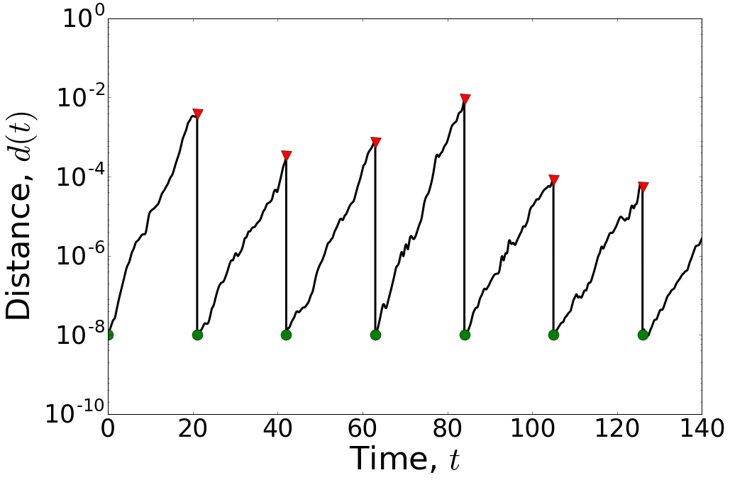
(b)

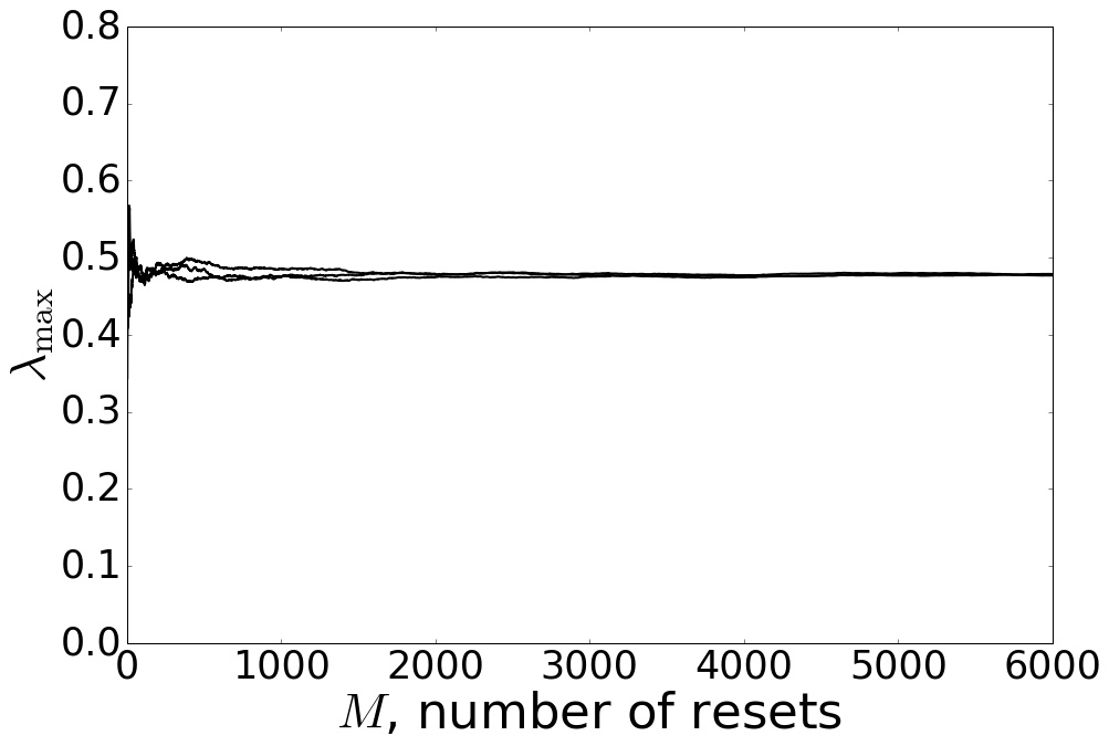
Figure 2: (Color online) Illustrations of the numerical routine for computing $\lambda_{\max}$. (a) Black line: distance $d(t)=\left\|\mathbf{R}_{1}(t)-\mathbf{R}_{2}(t)\right\|_{2}$ between two phase space trajectories $\mathbf{R}_{1}(t)$ and $\mathbf{R}_{2}(t)$ used for computing $\lambda_{\max}$ for DGPE on a one-dimensional lattice with $N=10$ sites. Time is divided into intervals of duration $T_{0}\approx 20$, each starts at the reset time $t_{m}$ (green dots), for which $d(t_{m})=d_{0}=10^{-8}$, and finishes at time $t_{m}+T_{0}$ (red triangles). According to Eq. (7), the contribution to $\lambda_{\max}$ from each such an interval (local stretching rate) is $\frac{1}{T_{0}}\log\left|\frac{d(t_{m})}{d_{0}}\right|$. (b) Ergodicity test: lines represent $\lambda_{\max}$ obtained from Eq. (7) as a function of the number of resets $M$. Each line is obtained for different randomly-chosen initial conditions for $\mathbf{R}_{1}(t)$ on the same shell of constant $E_{total}$ and $N_{p}$. Convergence to a single value of $\lambda_{\max}$ with time indicates that the system is ergodic.

We mark all the variables corresponding to the time interval preceding the time-reversal at time $\tau$ with a subscript “$-$” and succeeding the time-reversal with a subscript “$+$”.

Loschmidt echo is implemented as follows. The time evolution of the system during time interval $[0,\tau]$ is governed by the Hamiltonian ${\cal H}_{-}$ (3) and, after time $\tau$, by the sign-reversed Hamiltonian $\mathcal{H}_{+}=-{\cal H}_{-}$, i.e. we change the sign of the Hamiltonian parameters at time $\tau$: $J_{+}=-J_{-}$, $\beta_{+}=-\beta_{-}$. How to realize such a time-reversal experimentally will be discussed in Section VI.3. At the moment of time reversal, we also introduce a tiny perturbation to the state vector: $\psi_{i}(\tau+0)=\psi_{i}(\tau-0)+\delta\psi_{i}$, where $\left\{\delta\psi_{i}\right\}$ is a random vector, subject to the constraint $\sqrt{\sum_{i}\left|\delta\psi_{i}\right|^{2}}=10^{-8}$.

We have chosen a set of on-site occupations $n_{i}\equiv\left|\psi_{i}^{2}\right|$ as the quantity of interest $\mathbf{X}(t)\equiv\{n_{1},n_{2},\ldots,n_{N}\}$. Thus, we characterize Loschmidt echo by the function $G(\Delta t)\equiv\left\langle\log\left|\mathbf{X}(\tau+\Delta t)-\mathbf{X}(\tau-\Delta t)\right|\right\rangle$, which for the for the chosen quantity of interest can be written as

$$G(\Delta t)=\left\langle\log\sqrt{\sum_{i=1}^{N}\left[\Delta n_{i}(\Delta t)\right]^{2}}\right\rangle,$$ (4)

where $\Delta n_{i}(\Delta t)\equiv n_{i}(\tau+\Delta t)-n_{i}(\tau-\Delta t)$, and $\left\langle\ldots\right\rangle$ denotes ensemble averaging over initial conditions. As explained in Section II, the regime of the exponential growth of perturbation is expected to be characterized by the asymptotic relation

$$G(\Delta t)\cong\lambda_{\max}\Delta t,$$ (5)

from which the value of the largest Lyapunov exponent can be extracted. In the following sections, we demonstrate the validity of the above proposition by, first, directly calculating $\lambda_{\max}$ according to the algorithm of Ref. Sprott and Sprott (2003), and then comparing it with the value extracted from Eq. (5) on the basis of direct simulations of Loschmidt echoes.

We will do this for a one-dimensional lattice with $10$ sites, a two-dimensional square lattice of size $10\times 10$ and a three-dimensional cubic lattice of size $4\times 4\times 4$ with nearest-neighbor interactions and periodic boundary conditions.

IV Numerical algorithm

To simulate the solutions of DGPE, we employ a Runge-Kutta 4th order algorithm with discretization step $\delta t$=0.001. This limits the algorithmic error to $O(\delta t^{4})$ or roughly $10^{-12}$, whereas by using the quadrupole-precision numbers we fix the machine precision to be roughly $10^{-33}$.

The value of $\lambda_{\max}$ in general depends on the two conserved quantities of the system $E_{total}$ and $N_{p}$.

We generate an ensemble of initial conditions corresponding to $E_{total}=100N$ and $N_{p}=100N$, where $N$ is the number of lattice sites. We do this by choosing initially all $\left|\psi_{i}\right|=10$, with random phases. Then, we minimize $\left(E_{total}-100N\right)^{2}+\left(N_{p}-100N\right)^{2}$ by the steepest descent optimization procedure.

As mentioned in Section III, we introduce a small perturbation at the moment of time-reversal by adding a random perturbation $\left\{\delta\psi_{i}\right\}$ to the state vector $\left\{\psi_{i}\right\}$. The length of the perturbation vector is $10^{-8}$. This procedure slightly changes $E_{total}$ and $N_{p}$, but the resulting difference in the value of the largest Lyapunov exponent is several orders of magnitude smaller than the chosen precision of $3$ significant digits. Therefore, we can neglect it.

For further details one can refer to the source code published in a GitHub repository .

IV.1 Lyapunov exponent calculation

The definition of the largest Lyapunov exponent reads

$$\lambda_{\max}\equiv\frac{1}{t}\lim\left(\log\left|\frac{d(t)}{d(0)}\right|\right)_{t\to\infty,d(0)\to 0},$$ (6)

where $d(t)=\left\|\mathbf{R}_{1}(t)-\mathbf{R}_{2}(t)\right\|_{2}$ is the distance between two phase space trajectories, which are infinitesimally close to each other at $t=0$.

This definition is not practical for numerical simulation because it in general requires unachievable computational precision. Instead, we perform the direct calculation of the largest Lyapunov exponent $\lambda_{\max}$ following the standard numerical algorithm, see e.g. Ref. Wimberger (2014).

This algorithm tracks two trajectories: the reference trajectory $\mathbf{R}_{1}(t)$ and the slightly perturbed trajectory $\mathbf{R}_{2}(t)=\mathbf{R}_{1}(t)+\mathbf{\delta R}(t)$. The algorithm starts with $\left|\mathbf{\delta R}(0)\right|=d_{0}$ and then lets $\mathbf{\delta R}(t)$ grow during time interval $T_{0}$, then it shifts $\mathbf{R}_{2}(t)$ closer to $\mathbf{R}_{1}(t)$ by resetting the length of $\mathbf{\delta R}$ back to $d_{0}$. This procedure is repeated as many times as necessary, until the following quantity converges:

$$\lambda_{max}=\frac{1}{MT_{0}}\sum_{m}^{M}\log\left|\frac{d(t_{m})}{d_{0}}\right|,$$ (7)

where $M$ is the number of resets, $m$ is the reset index, $t_{m}$ is the time just before the $m$-th reset. The time evolution of the distance $d(t)$ in the course of such simulation is presented in Fig. 2(a).

In all our simulations we test the ergodicity of system’s dynamics numerically by checking that the values of $\lambda_{\max}$ obtained for several randomly chosen initial conditions on a shell with the given values of $E_{total}$ and $N_{p}$ are the same. In all cases reported below, this ergodicity test was positive. One such a test is illustrated in Fig. 2(b).

IV.2 Loschmidt echo simulations

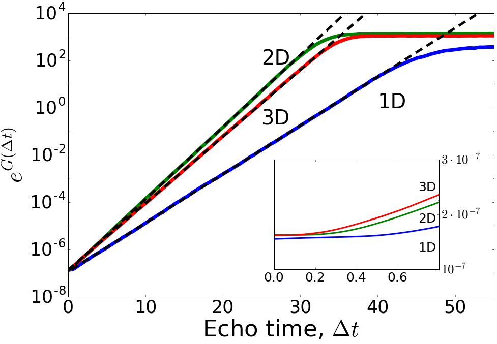
Figure 3: (Color online) Loschmidt echo response $\exp\left(G(\Delta t)\right)$ obtained from Eq. (4) for a one-dimensional chain of $10$ sites (1D, blue line), a two-dimensional $10\times 10$ square lattice (2D, green line) and a three-dimensional $4\times 4\times 4$ cubic lattice (3D, red line). The inset shows the behavior of $\exp\left(G(\Delta t)\right)$ in the transient regime at small echo times, where all Lyapunov exponents contribute to the growth. The transient regime takes longer time for lower dimensions. In Table 1, the values of $\lambda_{\max}$ obtained by fitting the exponential growth regime are compared to those obtained from the direct calculation described in Section IV.1.

We have computed the Loschmidt echo response function $G(\Delta t)$ given by Eq. (4) for one-, two- and three-dimensional lattice geometries with the parameters defined in Section III. The results of these simulations are presented in Fig. 3.

As clearly seen in Fig. 3, the expected exponential growth regime of $G(\Delta t)$ is present in all three cases. The values of $\lambda_{\max}$ characterizing this regime are summarized in Table. 1, where they are also compared with the values of $\lambda_{\max}$ obtained from the direct calculation described in Section IV.1. The agreement between the two sets of values is within the numerical accuracy of the calculations. Similar agreement was demonstrated previously in Ref. Fine et al. (2014) for classical spins. We finally note here that the fact that the largest Lyapunov exponent for the 3D cubic lattice is slightly smaller than that for the 2D square lattice is presumably a finite size effect related to the small size of the 3D lattice.

	$\lambda_{\max}$ from direct calculation	$\lambda_{\max}$ from Loschmidt echo
1D	$0.481\pm 0.002$	$0.475\pm 0.004$
2D	$0.703\pm 0.003$	$0.702\pm 0.004$
3D	$0.648\pm 0.002$	$0.650\pm 0.003$

Table 1: Comparison of the largest Lyapunov exponents $\lambda_{\max}$ obtained from the direct calculation with those extracted from Loschmidt echoes shown in Fig. 3 for one-, two- and three-dimensional lattices.

V Applicability of DGPE as a constraint on experimental implementation

Throughout the paper we used DGPE to model the dynamics of Bose-Einstein condensates on a lattice. In order to observe experimentally the regime of exponential growth $G(\Delta t)$ and to extract from this regime the value of $\lambda_{\max}$, the measured system should be such that DGPE approximates its dynamics with a very high accuracy. The question then arises whether such an accuracy is feasible for realistic experimental settings. To address this question, let us recall that DGPE is normally justified for the lattices of Bose-Einstein condensates by describing it at a level of a more fundamental Bose-Hubbard model. Therefore, we have to define the experimental regime, where both conditions would be satisfied simultaneously: the Bose-Hubbard model would be applicable and the classical mean-field approximation to it would be sufficiently accurate.

The Bose-Hubbard model is defined by the Hamiltonian

$$\hat{{\cal H}}_{BH}=-J\sum_{\left\langle i,j\right\rangle}\hat{a}_{i}^{+}\hat{a}_{j}+\frac{\beta}{2}\sum_{i}\hat{n}_{i}\hat{n}_{i},$$ (8)

where $\hat{a}_{i}^{+}$ and $\hat{a}_{i}$ are the quantum creation and annihilation operators for site $i$ respectively, $\hat{n}_{i}\equiv\hat{a}_{i}^{+}\hat{a}_{i}$ is the operator for the occupation at site $i$, $J$ is the hopping parameter, $\beta$ is the on-site interaction parameter, and the notation $\left\langle i,j\right\rangle$ implies nearest-neighbor sites. When the number of bosons in each potential well is large, one can approximate the Bose-Hubbard Hamiltonian (8) with the DGPE Hamiltonian (3) by making the following substitution: $\hat{a}_{i}=\psi_{i}$, $\hat{a}_{i}^{+}=\psi_{i}^{*}$, $\hat{n}_{i}=n_{i}=\left|\psi_{i}\right|^{2}$.

For the single-orbital Bose-Hubbard model to be valid, the hopping term $J$ must be relatively small, so that the lattice potential is deep enough and, as a result, the gap $\Delta_{0}$ between the lowest and the second lowest bands is sufficiently large Morsch and Oberthaler (2006); Bloch et al. (2008). In addition, in order for a Lyapunov instability to be observable, not only the order-parameters $\psi_{i}$ but also small deviations $\delta\psi_{i}$ should be well defined in the mean-field approximation, which implies sufficiently large values of $n_{i}$. The implementation of our proposal then requires the following conditions to be satisfied: (i) $J\ll\Delta_{0}$ — the condition for not involving the second band, (ii) $\beta n_{j}\lesssim J$ — the condition preventing the system from exhibiting self-trapping Milburn et al. (1997); Smerzi et al. (1997); Raghavan et al. (1999); Leggett (2001); Albiez et al. (2005); Khomeriki et al. (2007), (iii) ideally, the number of particles per well $n_{i}$ should be of the order of $500$ or larger Morsch and Oberthaler (2006); Bloch et al. (2008); Vardi and Anglin (2001). We note here that (ii) together with (iii) imply that the condition for the validity of the mean-field approximation in the Bose-Hubbard model, $\beta/J\ll 1$, is automatically fulfilled. It should be possible to satisfy all the above conditions with an optical lattice having potential depth of the order of $5\div 10$ recoil energies and not too strong interactions between atoms Holthaus (2000). We also note that the numerical experience with large quantum spins Elsayed and Fine (2015) indicates that even $n_{i}\sim 15$ might be already sufficient to extract the largest Lyapunov exponent.

VI Experimental Proposal

An experiment implementing our proposal should satisfy the following requirements: (i) high accuracy of the measurements of the number of particles $n_{i}$ for individual sites leading to the high accuracy of $G(\Delta t)$ extracted from these measurements, (ii) high accuracy of the experimental realization of the time-reversed Hamiltonian and (iii) high accuracy of the DGPE approximation for the given experimental setting. The relative accuracy in each case should be at least $10^{-2}$ and preferably better. Let us now consider the above requirements one by one.

VI.1 Measurement of the quantity of interest

In order to extract $G(\Delta t)$ from experiment, the initial and the final values of $n_{i}$ should be measured with high accuracy. In principle, there exist techniques, such as the absorption imaging Muessel et al. (2013) or the resonant fluorescence detection Hume et al. (2013) that allow one to achieve the required accuracy. In particular, the current state-of-the-art record for the resonant fluorescence detection Hume et al. (2013) is to measure the number of atoms of the order of one thousand with accuracy better than one percent. However, our proposal implies an additional requirement, namely, that the initial measurement should not significantly perturb $n_{i}$, so that the measured values represent the initial conditions for the actual experimental run. This implies that destructive techniques, such as absorption imaging, would not be suitable for the initial measurement, because they would destroy the condensate. Therefore, it is preferable that at least the initial measurement is performed by a non-destructive technique, such as, e.g., dispersive (off-resonance) imaging Andrews et al. (1996); Miesner et al. (1998) or the techniques used in Refs. Wilson et al. (2015); Figl et al. (2006). The alternative approach would be to controllably prepare the initial state with an accurate a priori knowledge of the initial number of particles on each site. The final measurement can then be done by either destructive or non-destructive imaging technique.

VI.2 Initial and final conditions

We propose to create the optical lattice initially with sufficiently high potential barriers between adjacent sites, which would suppress hopping between them while the initial occupations are measured. Then, the barriers should be lowered to the heights corresponding to the desired value of the hopping parameter $J$. The barriers should be lowered sufficiently fast, so that the initial occupations of individual wells remain the same. At the same time, after the barriers are lowered the initial phases of individual order-parameters $\psi_{i}$ are expected to be random. Thereby an ensemble of random initial conditions is to be implemented. After this, both the direct and the reversed time evolution should last for a time $\tau$ each. Then, the barriers should be raised again, so that the final occupations of individual wells can be measured slowly and accurately.

VI.3 Time-reversal of dynamics

In order to reverse the sign of the Hamiltonian $\mathcal{H}$ (3) at time $\tau$, one can change the sign of the hopping parameter $J$ and the interaction parameter $\beta$.

The sign-reversal of $J$ can be implemented using fast periodic shaking of the optical lattice. As shown in Refs. Eckardt et al. (2005); Lignier et al. (2007); Struck et al. (2011), the effective hopping parameter $J$ depends on the periodic forcing amplitude $F$ and the modulation frequency $\omega$ as follows:

$$J(F,\omega)={\cal J}_{0}\left(\frac{d\left|F\right|}{\hbar\omega}\right)\tilde{J},$$ (9)

where ${\cal J}_{0}$ is the zeroth order Bessel function, $\tilde{J}$ is the bare hopping parameter and $d$ is the lattice spacing. Since ${\cal J}_{0}$ is a sign-alternating function, one can find pairs of parameters $F_{1}$, $\omega_{1}$ and $F_{2}$, $\omega_{2}$, such that $J(F_{2},\omega_{2})=-J(F_{1},\omega_{1})$. Such a time-reversal can be implemented on the timescale of the order of the modulation frequency $\omega$, which is several kHz Sias et al. (2007); Zenesini et al. (2009); Struck et al. (2011).

The sign-reversal of the interaction parameter $\beta$ can be implemented with the help of Feshbach resonances Feshbach (1958); Inouye et al. (1998). This parameter is proportional to the atomic $s$-wave scattering length $a_{sc}$, whose value and sign can be controlled by the value of external magnetic field $B$. Cesium or rubidium 85 could be good candidates for this kind of experiment, due to their broad Feshbach resonances Roberts et al. (1998); Claussen et al. (2003); Gustavsson et al. (2008). In this case, the on-site interaction can be reversed on a timescale of fractions of ms.

According to the above proposal, the time-reversal of the effective Hamiltonian $\mathcal{H}$ can be implemented within a fraction of ms, whereas the system dynamics controlled by the values of $J$ and $\beta$ can be at least one order of magnitude slower.

Bose-Einstein condensates with attractive interaction (which will be required either for the forward or the backward time-evolution) are in general unstable to collapse. However, if they are constrained to a finite volume, the collapse happens only for numbers of atoms above a certain critical value, which for realistic optical lattice parameters can be above 1000 per lattice site Sackett et al. (1999); Gerton et al. (2000); Donley et al. (2001); Khaykovich et al. (2002); Strecker et al. (2002); Eigen et al. (2016). As mentioned earlier, the implementation of our proposal requires about 500 atoms per lattice site.

Another useful possibility that potentially improves the flexibility of experimental implementation is to achieve the time-reversal not by realizing the strict condition $\mathcal{H}_{+}=-\mathcal{H}_{-}$, but, instead, borrowing the idea from the magic echo of nuclear magnetic resonance Rhim et al. (1970); Slichter (2013), to change the sign of $J$ and $\beta$ in such a way that the Hamiltonian before the time-reversal $J_{-},\beta_{-}$ are related to the parameters after the time-reversal $J_{+},\beta_{+}$ as follows: $J_{+}=-CJ_{-}$, $\beta_{+}=-C\beta_{-}$, where $C$ is some positive constant. In such a case, $\mathcal{H}_{+}=-C\mathcal{H}_{-}$, so that the time-reversal routine would consist of the direct time-evolution taking time $\tau$ and the reversed time-evolution taking time $\tau/C$.

VI.4 Lattice geometry

Experimentally realized optical lattices are, normally, not quite translationally invariant because of the presence of physical borders. This, in particular, leads to an effective position-dependent on-site potential and/or position-dependent hopping, whose values near the borders of the lattice are different from those in the bulk. In such a case, the time-reversal of the full Hamiltonian requires reversing the sign of the above position-dependent terms, which, in turn, poses an additional experimental complication. It is, therefore, preferable for implementing our proposal to use an optical lattice that actually has periodic boundary conditions, which, for all practical purposes, leaves us with a ring-shaped one-dimensional lattice. Such a lattice can be realized, for example, on the basis of an interference pattern of two Laguerre-Gauss modes with different orbital indices Franke-Arnold et al. (2007); Amico et al. (2014).

VII Conclusions

We proposed a method to extract the largest Lyapunov exponent for a lattice of Bose-Einstein condensates on the basis of a Loschmidt echo routine. We have validated this method by numerical simulations and discussed its possible experimental implementation with ultracold bosonic atoms in optical lattices. A successful realization of this proposal may produce a long-sought direct experimental evidence that the dynamics of a typical many-particle system is chaotic. This, in turn, would put the theory of dynamic thermalization on a firmer foundation.