Look, Listen and Learn

Abstract

We consider the question: what can be learnt by looking at and listening to a large number of unlabelled videos? There is a valuable, but so far untapped, source of information contained in the video itself – the correspondence between the visual and the audio streams, and we introduce a novel “Audio-Visual Correspondence” learning task that makes use of this. Training visual and audio networks from scratch, without any additional supervision other than the raw unconstrained videos themselves, is shown to successfully solve this task, and, more interestingly, result in good visual and audio representations. These features set the new state-of-the-art on two sound classification benchmarks, and perform on par with the state-of-the-art self-supervised approaches on ImageNet classification. We also demonstrate that the network is able to localize objects in both modalities, as well as perform fine-grained recognition tasks.

1 Introduction

Visual and audio events tend to occur together; not always but often: the movement of fingers and sound of the instrument when a piano, guitar or drum is played; lips moving and speech when talking; cars moving and engine noise when observing a street. The visual and audio events are concurrent in these cases because there is a common cause. In this paper we investigate whether we can use this simple observation to learn about the world both visually and aurally by simply watching and listening to videos.

We ask the question: what can be learnt by training visual and audio networks simultaneously to predict whether visual information (a video frame) corresponds or not to audio information (a sound snippet)? This is a looser requirement than that the visual and audio events occur in sync. It only requires that there is something in the image that correlates with something in the audio clip – a car present in the video frame, for instance, correlating with engine noise; or an exterior shot with the sound of wind.

Our motivation for this work is three fold: first, as in many recent self-supervision tasks [8, 6, 1, 35, 36, 20, 24, 21], it is interesting to learn from a virtually infinite source of free supervision (video with visual and audio modes in this case) rather than requiring strong supervision; second, this is a possible source of supervision that an infant could use as their visual and audio capabilities develop; third, we want to know what can be learnt, and how well the networks are trained, for example in the performance of the visual and audio networks for other tasks.

Of course, we are not the first to make the observation that visual and audio events co-occur, and to use their concurrence or correlation as supervision for training a network. In a series of recent and inspiring papers [22, 23, 2, 11], the group at MIT has investigated precisely this. However, their goal is always to train a single network for one of the modes, for example, train a visual network to generate sounds in [22, 23]; or train an audio network to correlate with visual outputs in [2, 11], where the visual networks are pre-trained and fixed and act as a teacher. In earlier, pre deep-learning, approaches the observation was used to beautiful effect in [14] showing “pixels that sound” (e.g. for a guitar) learnt using CCA. In contrast, we train both visual and audio networks and, somewhat surprisingly, show that this is beneficial – in that our performance improves substantially over that of [2] when trained on the same data.

In summary: our goal is to design a system that is able to learn both visual and audio semantic information in a completely unsupervised manner by simply looking at and listening to a large number of unlabelled videos. To achieve this we introduce a novel Audio-Visual Correspondence (AVC) learning task that is used to train the two (visual and audio) networks from scratch. This task is described in section 2, together with the network architecture and training procedure. In section 3 we describe what semantic information has been learnt, and assess the performance of the audio and visual networks. We find, which we had not anticipated, that this task leads to quite fine grained visual and audio discrimination, e.g. into different instruments. In terms of quantitative performance, the audio network exceed those recently trained for audio recognition using visual supervision, and the visual network has similar performance to those trained for other, purely visual, self-supervision tasks. Furthermore, we show, as an added benefit, that we are able to localize the source of the audio event in the video frame (and also localize the corresponding regions of the sound source) using activation visualization.

In terms of prior work, the most closely related deep learning approach that we know of is ‘SyncNet’ in [5]. However, [5] is aimed at learning to synchronize lip-regions and speech for lip-reading, rather than the more general video and audio material considered here for learning semantic representations. More generally, the AVC task is a form of co-training [4], where there are two ‘views’ of the data, and each view provides complementary information. In our case the two views are visual and audio (and each can determine semantic information independently). A similar scenario arises when the two views are visual and language (text) as in [9, 18, 31] where a common embedding is learnt. However, usually one (or both) of the networks (for images and text) are pre-trained, in contrast to the approach taken here where no supervision is required and both networks are trained from scratch.

2 Audio-visual correspondence learning

The core idea is to use a valuable but so far untapped source of information contained in the video itself – the correspondence between visual and audio streams available by virtue of them appearing together at the same time in the same video. By seeing and hearing many examples of a person playing a violin and examples of a dog barking, and never, or at least very infrequently, seeing a violin being played while hearing a dog bark and vice versa, it should be possible to conclude what a violin and a dog look and sound like, without ever being explicitly taught what is a violin or a dog.

Figure 1: Audio-visual correspondence task (AVC). A network should learn to determine whether a pair of (video frame, short audio clip) correspond to each other or not. Positives are (frame, audio) extracted from the same time of one video, while negatives are a frame and audio extracted from different videos.

We leverage this for learning by an audio-visual correspondence (AVC) task, illustrated in Figure 1. The AVC task is a simple binary classification task: given an example video frame and a short audio clip – decide whether they correspond to each other or not. The corresponding (positive) pairs are the ones that are taken at the same time from the same video, while mismatched (negative) pairs are extracted from different videos. The only way for a system to solve this task is if it learns to detect various semantic concepts in both the visual and the audio domain. Indeed, we demonstrate in Section 3.5 that our network automatically learns relevant semantic concepts in both modalities.

It should be noted that the task is very difficult. The network is made to learn visual and audio features and concepts from scratch without ever seeing a single label. Furthermore, the AVC task itself is quite hard when done on completely unconstrained videos – videos can be very noisy, the audio source is not necessarily visible in the video (e.g. camera operator speaking, person narrating the video, sound source out of view or occluded, etc.), and the audio and visual content can be completely unrelated (e.g. edited videos with added music, very low volume sound, ambient sound such as wind dominating the audio track despite other audio events being present, etc.). Nevertheless, the results in Section 3 show that our network is able to fairly successfully solve the AVC task, and in the process learn very good visual and audio representations.

2.1 Network architecture

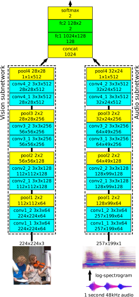
Figure 2: $L^{3}$-Net architecture. Each blocks represents a single layer with text providing more information – first row: layer name and parameters, second row: output feature map size. Layers with a name prefix conv, pool, fc, concat, softmax are convolutional, max-pooling, fully connected, concatenation and softmax layers, respectively. The listed parameters are: conv – kernel size and number of channels, pooling – kernel size, fc – size of the weight matrix. The stride of pool layers is equal to the kernel size and there is no padding. Each convolutional layer is followed by batch normalization [12] and a ReLU nonlinearity, and the first fully connected layer (fc1) is followed by ReLU.

To tackle the AVC task, we propose the network structure shown in Figure 2. It has three distinct parts: the vision and the audio subnetworks which extract visual and audio features, respectively, and the fusion network which takes these features into account to produce the final decision on whether the visual and audio signals correspond. Here we describe the three parts in more detail.

Vision subnetwork.

The input to the vision subnetwork is a $224\times 224$ colour image. We follow the VGG-network [30] design style, with $3\times 3$ convolutional filters, and $2\times 2$ max-pooling layers with stride $2$ and no padding. The network can be segmented into four blocks of conv+conv+pool layers such that inside each block the two conv layers have the same number of filters, while consecutive blocks have doubling filter numbers: 64, 128, 256 and 512. At the very end, max-pooling is performed across all spatial locations to produce a single 512-D feature vector. Each conv layer is followed by batch normalization [12] and a ReLU nonlinearity.

Audio subnetwork.

The input to the audio subnetwork is a 1 second sound clip converted into a log-spectrogram (more details are provided later in this section), which is thereafter treated as a greyscale $257\times 199$ image. The architecture of the audio subnetwork is identical to the vision one with the exception that input pixels are 1-D intensities instead of 3-D colours and therefore the conv1_1 filter sizes are $3\times$ smaller compared to the vision subnetwork. The final audio feature is also 512-D.

Fusion network.

The two 512-D visual and audio features are concatenated into a 1024-D vector which is passed through the fusion network to produce a 2-way classification output, namely, whether the vision and audio correspond or not. It consists of two fully connected layers, with ReLU in between them, and the intermediate feature size of 128-D.

2.2 Implementation details

Training data sampling.

A non-corresponding frame-audio pair is compiled by randomly sampling two different videos and picking a random frame from one and a random 1 second audio clip from the other. A corresponding frame-audio pair is created by sampling a random video, picking a random frame in that video, and then picking a random 1 second audio clip that overlaps in time with the sampled frame. This provides additional training samples compared to simply sampling the 1 second audio with the frame at its mid-point. We use standard data augmentation techniques for images: each training image is uniformly scaled such that the smallest dimension is equal to 256, followed by random cropping into $224\times 224$, random horizontal flipping, and brightness and saturation jittering. Audio is only augmented by changing the volume up to 10% randomly but consistently across the sample.

Log-spectrogram computation.

The 1 second audio is resampled to 48 kHz, and a spectrogram is computed with window length of 0.01 seconds and a half-window overlap; this produces 199 windows with 257 frequency bands. The response map is passed through a logarithm before feeding it into the audio subnetwork.

Training procedure.

We use the Adam optimizer [15], weight decay $10^{-5}$, and perform a grid search on the learning rate, although $10^{-4}$ usually works well. The network was trained on 16 GPUs in parallel with synchronous training implemented in TensorFlow, where each worker processed a 16-element batch, thus making the effective batch size of 256. For a training set of 400k 10 second videos, the network is trained for two days, during which it has seen 60M frame-audio pairs.

3 Results and discussion

Our “look, listen and learn” network ($L^{3}$-Net) approach is evaluated and examined in multiple ways. First, the performance of the network on the audio-visual correspondence task itself is investigated, and compared to supervised baselines. Second, the quality of the learnt visual and audio features is tested in a transfer learning setting, on visual and audio classification tasks. Finally, we perform a qualitative analysis of what the network has learnt. We start by introducing the datasets used for training.

3.1 Datasets

Two video datasets are used for training the networks: Flickr-SoundNet and Kinetics-Sounds.

Flickr-SoundNet [2].

This is a large unlabelled dataset of completely unconstrained videos from Flickr, compiled by searching for popular tags, but no tags or any sort of additional information apart from the videos themselves are used. It contains over 2 million videos but for practical reasons we use a random subset of 500k videos (400k training, 50k validation and 50k test) and only use the first 10 seconds of each video. This is the dataset that is used for training the $L^{3}$-Net for the transfer learning experiments in Sections 3.3 and 3.4.

Kinetics-Sounds.

While our goal is to learn from completely unconstrained videos, having a labelled dataset is useful for quantitative evaluation. For this purpose we took a subset (much smaller than Flickr-SoundNet) of the Kinetics dataset [13], which contains YouTube videos manually annotated for human actions using Mechanical Turk, and cropped to 10 seconds around the action. The subset contains 19k 10 second video clips (15k training, 1.9k validation, 1.9k test) formed by filtering the Kinetics dataset for 34 human action classes, which have been chosen to be potentially manifested visually and aurally, such as playing various instruments (guitar, violin, xylophone, etc.), using tools (lawn mowing, shovelling snow, etc.), as well as performing miscellaneous actions (tap dancing, bowling, laughing, singing, blowing nose, etc.); the full list is given in appendix A. Although this dataset is fairly clean by construction, it still contains considerable noise, e.g. the bowling action is often accompanied by loud music at the bowling alley, human voices (camera operators or video narrations) often masks the sound of interest, and many videos contain sound tracks that are completely unrelated to the visual content (e.g. music montage for a snow shovelling video).

3.2 Audio-visual correspondence

First we evaluate the performance of our method on the task it was trained to solve – deciding whether a frame and a 1 second audio clip correspond (Section 2). For the Kinetics-Sounds dataset which contains labelled videos, we also evaluate two supervised baselines in order to gauge how well the AVC training compares to supervised training.

Supervised baselines.

For both baselines we first train vision and audio networks independently on the action classification task, and then combine them in two different ways. The vision network has an identical feature extraction trunk as our vision subnetwork (Section 2.1), on top of which two fully connected layers are attached (sizes: $512\times 128$ and $128\times 34$) to perform classification into the 34 Kinetics-Sounds classes. The audio classification network is constructed analogously. The direct combination baseline computes the audio-video correspondence score as the similarity of class score distributions of the two networks, computed as the scalar product between the 34-D network softmax outputs, and decides that audio and video are in correspondence if the score is larger than a threshold. The motivation behind this baseline is that if the vision network believes the frame contains a dog while the audio network is confident it hears a violin, then the (frame, audio) pair is unlikely to be in correspondence. The supervised pretraining baseline takes the feature extraction trunks from the two trained networks, assembles them into our network architecture by concatenating the features and adding two fully connected layers (Section 2.1). The weights of the feature extractors are frozen and the fully connected layers are trained on the AVC task in the same manner as our network. This is the strongest baseline as it directly corresponds to our method, but with features learnt in a fully supervised manner.

Method	Flickr-SoundNet	Kinetics-Sounds
Supervised direct	–	65%
Supervised pretraining	–	74%
$L^{3}$-Net	78%	74%

Table 1: Audio-visual correspondence (AVC) results. Test set accuracy on the AVC task for the $L^{3}$-Net, and the two supervised baselines on the labelled Kinetics-Sounds dataset. The number of positives and negatives is the same, so chance gets 50%. All methods are trained on the training set of the respective datasets.

Results and discussion.

Table 1 shows the results on the AVC task. The $L^{3}$-Net achieves 74% and 78% on the two datasets, where chance is 50%. It should be noted that the task itself is quite hard due to the unconstrained nature of the videos (Section 2), as well as due to the very local input data which lacks context – even humans find it hard to judge whether an isolated frame and an isolated single second of audio correspond; informal human tests indicated that humans are only a few percent better than the $L^{3}$-Net. Furthermore, the supervised baselines do not beat the $L^{3}$-Net as “supervised pretraining” performs on par with it, while “supervised direct combination” works significantly worse as, unlike “supervised pretraining”, it has not been trained for the AVC task.

3.3 Audio features

In this section we evaluate the power of the audio representation that emerges from the $L^{3}$-Net approach. Namely, the $L^{3}$-Net audio subnetwork trained on Flickr-SoundNet is used to extract features from 1 second audio clips, and the effectiveness of these features is evaluated on two standard sound classification benchmarks: ESC-50 and DCASE.

Environmental sound classification (ESC-50) [26].

This dataset contains 2000 audio clips, 5 seconds each, equally balanced between 50 classes. These include animal sounds, natural soundscapes, human non-speech sounds, interior/domestic sounds, and exterior/urban noises. The data is split into 5 predefined folds and performance is measured in terms of mean accuracy over 5 leave-one-fold-out evaluations.

Detection and classification of acoustic scenes and events (DCASE) [32].

We consider the scene classification task of the challenge which contains 10 classes (bus, busy street, office, open air market, park, quiet street, restaurant, supermarket, tube, tube station), with 10 training and 100 test clips per class, where each clip is 30 seconds long.

(a) ESC-50	(b) DCASE
Method Accuracy SVM-MFCC [26] 39.6% Autoencoder [2] 39.9% Random Forest [26] 44.3% Piczak ConvNet [25] 64.5% SoundNet [2] 74.2% Ours random 62.5% Ours 79.3% Human perf. [26] 81.3%	Method Accuracy RG [27] 69% LTT [19] 72% RNH [28] 77% Ensemble [32] 78% SoundNet [2] 88% Ours random 85% Ours 93%

Table 2: Sound classification. “Ours random” is an additional baseline which shows the performance of our network without $L^{3}$-training. Our $L^{3}$-training sets the new state-of-the-art by a large margin on both benchmarks.

Method	Top 1 accuracy
Random	18.3%
Pathak et al. [24]	22.3%
Krähenbühl et al. [16]	24.5%
Donahue et al. [7]	31.0%
Doersch et al. [6]	31.7%
Zhang et al. [36] (init: [16])	32.6%
Noroozi and Favaro [21]	34.7%
Ours random	12.9%
Ours	32.3%

Table 3: Visual classification on ImageNet. Following [36], our features are evaluated by training a linear classifier on the ImageNet training set and measuring the classification accuracy on the validation set. For more details and discussions see Section 3.4. All performance numbers apart from ours are provided by authors of [36], showing only the best performance for each method over all parameter choices (e.g. Donahue et al. [7] achieve 27.1% instead of 31.0% when taking features from pool5 instead of conv3).

Experimental procedure.

To enable a fair direct comparison with the current state-of-the-art, Aytar et al. [2], we follow the same experimental setup. Multiple overlapping subclips are extracted from each recording and described using our features. For 5 second recordings from ESC-50 we extract 10 equally spaced 1 second subclips, while for the 6 times longer DCASE recordings, 60 subclips are extracted per clip. The audio features are obtained by max-pooling the last convolutional layer of the audio subnetwork (conv4_2), before the ReLU, into a $4\times 3\times 512=6144$ dimensional representation (the conv4_2 outputs are originally $16\times 12\times 512$). The features are preprocessed using z-score normalization, i.e. shifted and scaled to have a zero mean and unit variance. A multi-class one-vs-all linear SVM is trained, and at test time the class scores for a recording are computed as the mean over the class scores for its subclips.

Results and discussion.

Table 2 shows the results on ESC-50 and DCASE. On both benchmarks we convincingly beat the previous state-of-the-art, SoundNet [2], by 5.1% and 5% absolute. For ESC-50 we reduce the gap between the previous best result and the human performance by 72% while for DCASE we reduce the error by 42%. The results are especially impressive as SoundNet uses two vision networks trained in a fully supervised manner on ImageNet and Places2 as teachers for the audio network, while we learn both the vision and the audio networks without any supervision whatsoever. Note that we train our networks with a random subset of the SoundNet videos for efficiency purposes, so it is possible that further gains can be achieved by using all the available training data.

3.4 Visual features

In this section we evaluate the power of the visual representation that emerges from the $L^{3}$-Net approach. Namely, the $L^{3}$-Net vision subnetwork trained on Flickr-SoundNet is used to extract features from images, and the effectiveness of these features is evaluated on the ImageNet large scale visual recognition challenge 2012 [29].

Experimental procedure.

We follow the experimental setup of Zhang et al. [36] where features are extracted from $256\times 256$ images and used to perform linear classification on ImageNet. As in [36], we take conv4_2 features after ReLU and perform max-pooling with equal kernel and stride sizes until feature dimensionality is below 10k; in our case this results in $4\times 4\times 512=8192$-D features. A single fully connected layer is added to perform linear classification into the 1000 ImageNet classes. All the weights are frozen to their $L^{3}$-Net-trained values, apart from the final classification layer which is trained with cross-entropy loss on the ImageNet training set. The training procedure (data augmentation, learning rate schedule, label smoothing) is identical to [33], the only differences being that we use the Adam optimizer instead of RMSprop, and a $256\times 256$ input image instead of $299\times 299$ as it fits our architecture better and to be consistent with [36].

Fingerpicking	Lawn mowing	P. accordion	P. bass guitar	P. saxophone	Typing	Bowling	P. clarinet	P. organ

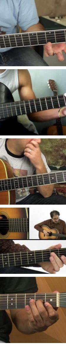
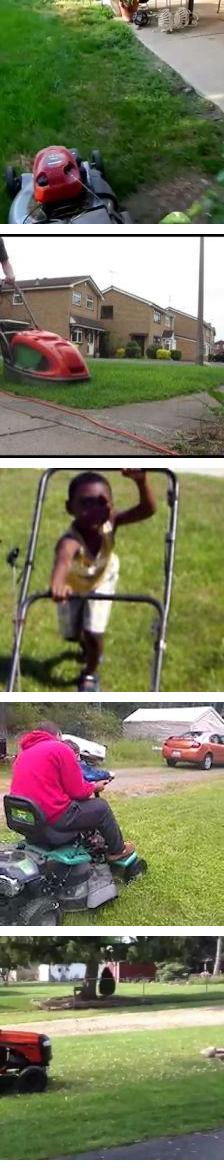
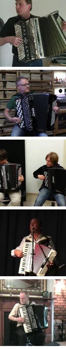
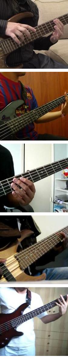
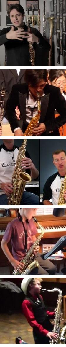
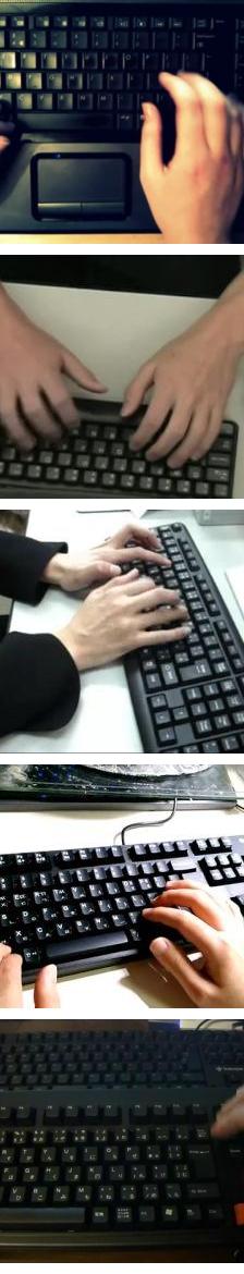
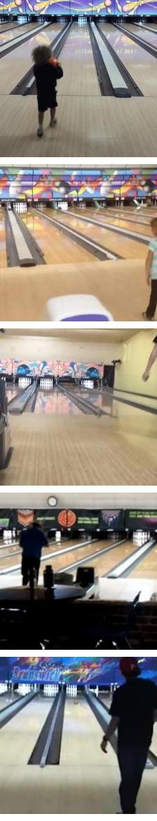
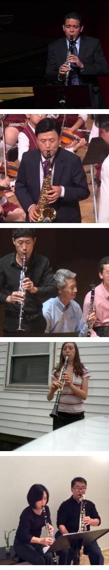
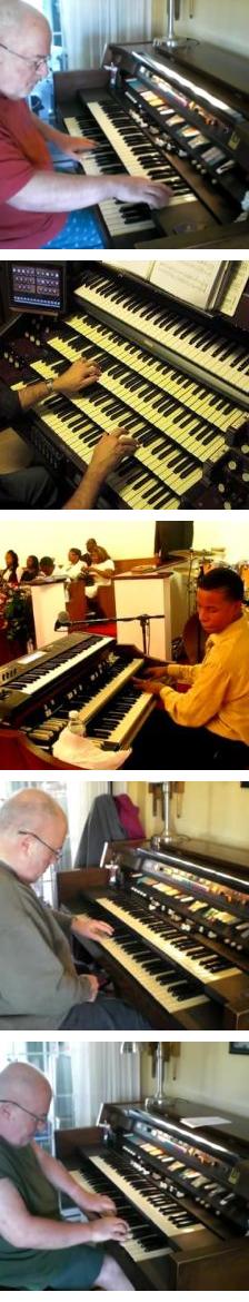
Figure 3: Learnt visual concepts (Kinetics-Sounds). Each column shows five images that most activate a particular unit of the 512 in pool4 for the vision subnetwork. Note that these features do not take sound as input. Videos come from the Kinetics-Sounds test set and the network was trained on the Kinetics-Sounds train set. The top row shows the dominant action label for the unit (“P.” stands for “playing”).

Fingerpicking	Lawn mowing	P. accordion	P. bass guitar	P. saxophone	Typing	Bowling	P. clarinet	P. organ

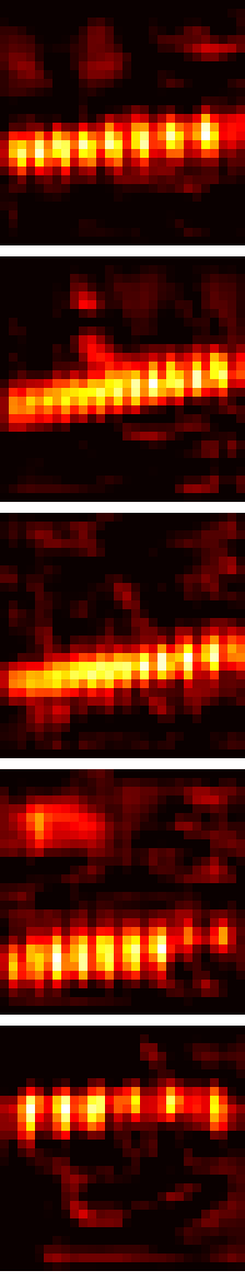
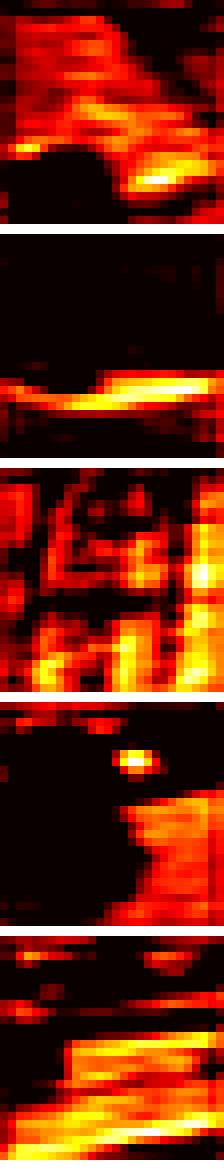
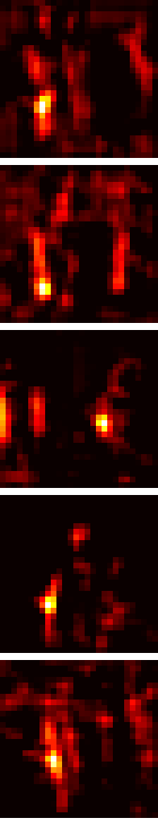
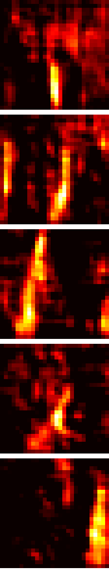
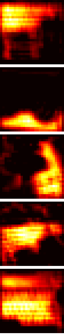
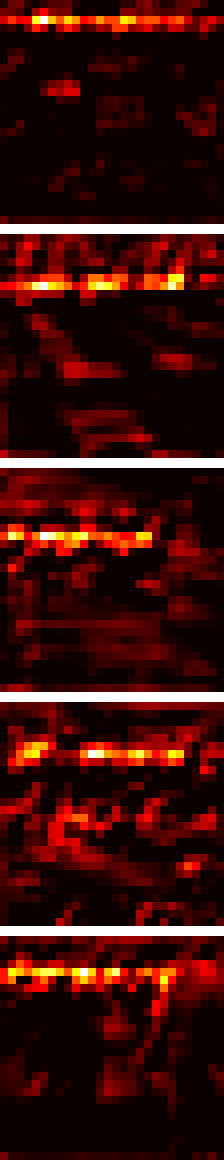
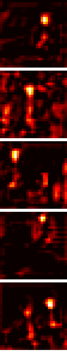
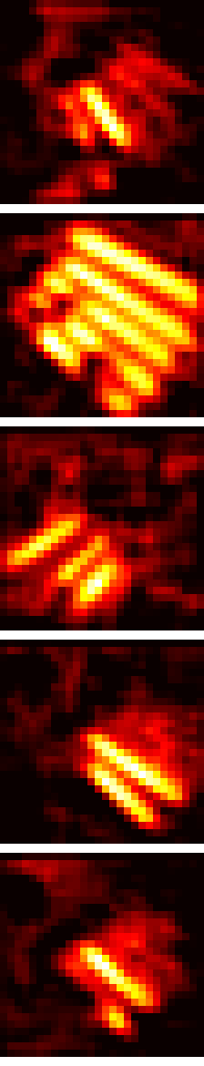
Figure 4: Visual semantic heatmap (Kinetics-Sounds). Examples correspond to the ones in Figure 3. A semantic heatmap is obtained as a slice of activations from conv4_2 of the vision subnetwork that corresponds to the same unit from pool4 as in Figure 3, i.e. the unit that responds highly to the class in question.

Results and discussion.

Classification accuracy on the ImageNet validation set is shown in Table 3 and contrasted with other unsupervised and self-supervised methods. We also test the performance of random features, i.e. our $L^{3}$-Net architecture without AVC training but with a trained classification layer.

Our $L^{3}$-Net-trained features achieve 32.3% accuracy which is on par with other state-of-the-art self-supervised methods of [6, 36, 7, 21], while convincingly beating random initialization, data-dependent initialization [16], and Context Encoders [24]. It should be noted that these methods use the AlexNet [17] architecture which is different to ours, so the results are not fully comparable. On the one hand, our architecture when trained from scratch in its entirety achieves a higher performance (59.2% vs AlexNet’s 51.0%). On the other hand, it is deeper which makes it harder to train as can be seen from the fact that our random features perform worse than theirs (12.9% vs AlexNet’s 18.3%), and that all competing methods hit peak performance when they use earlier layers (e.g. [7] drops from 31.0% to 27.1% when going from conv3 to pool5). In fact, when measuring the improvement achieved due to AVC or self-supervised training versus the performance of the network with random initialization, our AVC training beats all competitors.

Another important fact to consider is that all competing methods actually use ImageNet images when training. Although they do not make use of the labels, the underlying image statistics are the same: objects are fairly central in the image, and the networks have seen, for example, abundant images of 120 breads of dogs and thus potentially learnt their distinguishing features. In contrast, we use a completely separate source of training data in the form of frames from Flickr videos – here the objects are in general not centred, it is likely that the network has never seen a “Tibetan terrier” nor the majority of other fine-grained categories. Furthermore, video frames have vastly different low-level statistics to still images, with strong artefacts such as motion blur. With these factors hampering our network, it is impressive that our visual features $L^{3}$-Net-trained on Flickr videos perform on par with self-supervised state-of-the-art trained on ImageNet.

3.5 Qualitative analysis

In this section we analyse what is it that the network has learnt. We visualize the results on the test set of the Kinetics-Sounds and Flickr-SoundNet datasets, so the network has not seen the videos during training.

3.5.1 Vision features

To probe what the vision subnetwork has learnt, we pick a particular ‘unit’ in pool4 (i.e. a component of the 512 dimensional pool4 vector) and rank the test images by its magnitude. Figure 3 shows the images from Kinetics-Sounds that activate particular units in pool4 the most (i.e. are ranked highest by its magnitude). As can be seen, the vision subnetwork has automatically learnt, without any explicit supervision, to recognize semantic entities such as guitars, accordions, keyboards, clarinets, bowling alleys, lawns or lawnmowers, etc. Furthermore, it has learnt finer-grained categories as well as it is able to distinguish between acoustic and bass guitars (“fingerpicking” is mostly associated with acoustic guitars).

Figure 4 shows heatmaps for the Kinetics-Sounds images in Figure 3, obtained by simply displaying the spatial activations of the corresponding vision unit (i.e. if the $k$ component of pool4 is chosen, then the $k$ channel of conv4_2 is displayed – since the $k$ component is just the spatial max over this channel (after ReLU)). Objects are successfully detected despite significant clutter and occlusions. It is interesting to observe the type of cues that the network decides to use, e.g. the “playing clarinet” unit, instead of trying to detect the entire clarinet, seems to mostly activate on the interface between the player’s face and the clarinet.

Figures 5 and 6 show visual concepts learnt by the $L^{3}$-Net on the Flickr-SoundNet dataset. It can be seen that the network learns to recognize many scene categories (Figure 5), such as outdoors, concert, water, sky, crowd, text, railway, etc. These are useful for the AVC task as, for example, crowds indicate a large event that is associated with a distinctive sound as well (e.g. a football game), text indicates narration, and outdoors scenes are likely to be accompanied with wind sounds. It should be noted that though at first sight some categories seem trivially detectable, it is not the case; for example, “sky” detector is not equivalent to the “blueness” detector as it only fires on “sky” and not on “water”, and furthermore there are separate units sensitive to “water surface” and to “underwater” scenes. The network also learns to detect people as user uploaded content is substantially people-oriented – Figure 6 shows the network has learnt to distinguish between babies, adults and crowds.

Outdoor		Concert		Outdoor sport
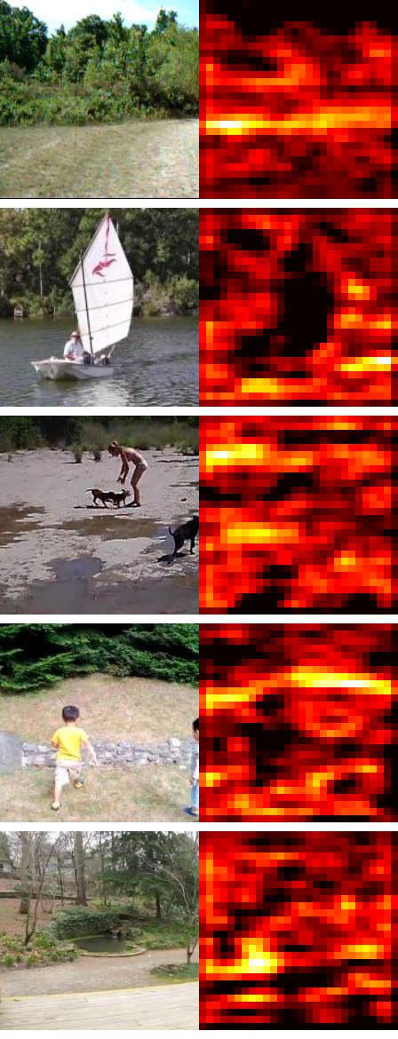
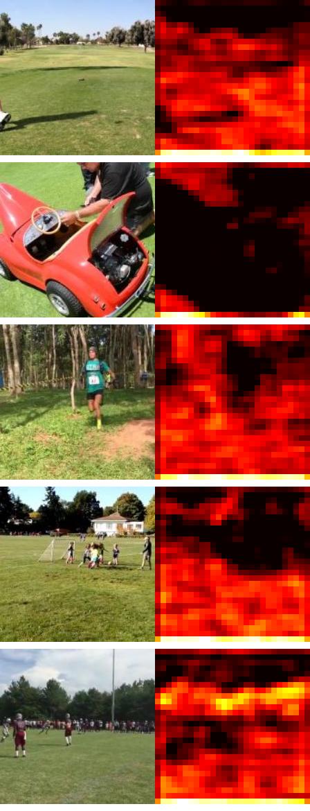
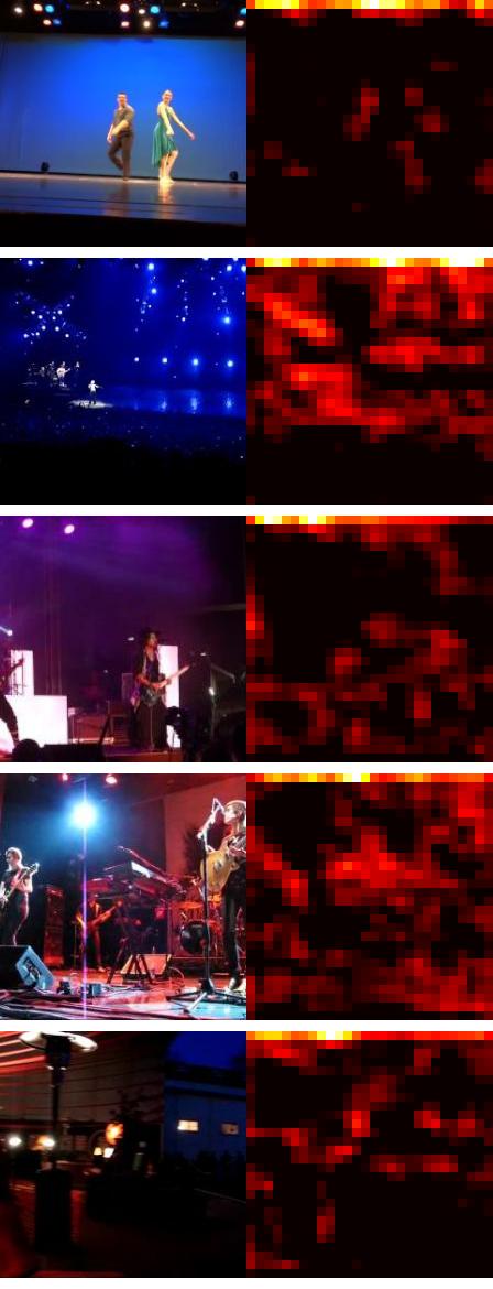
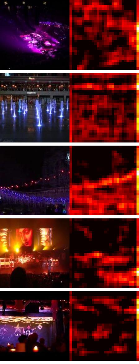
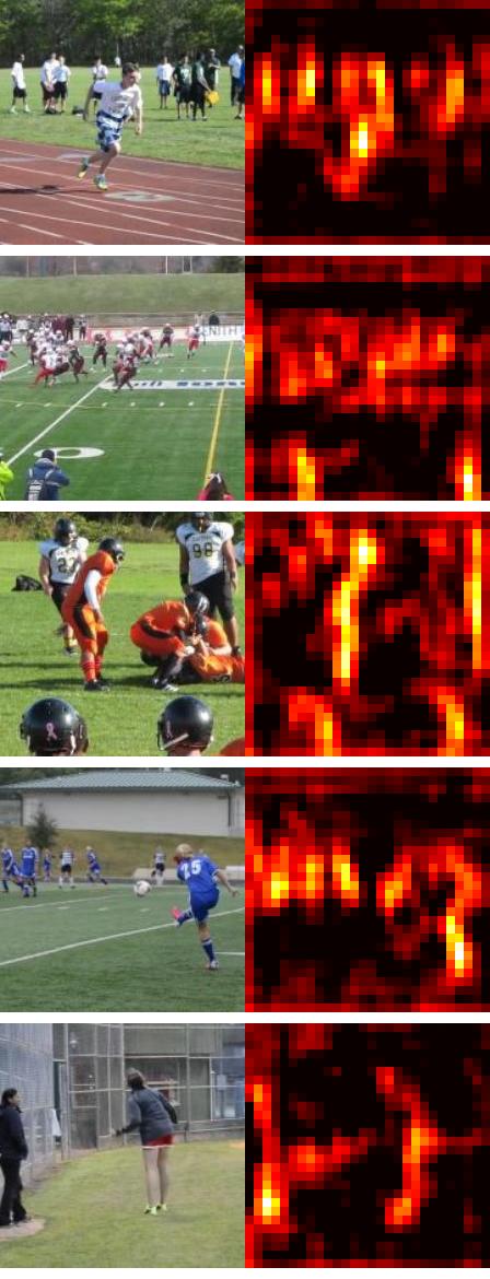
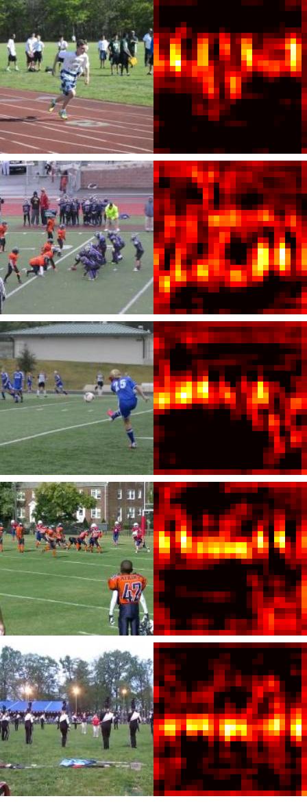
Cloudy sky	Sky		Water surface		Underwater
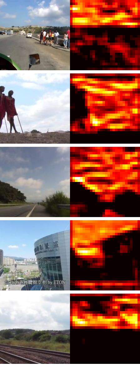
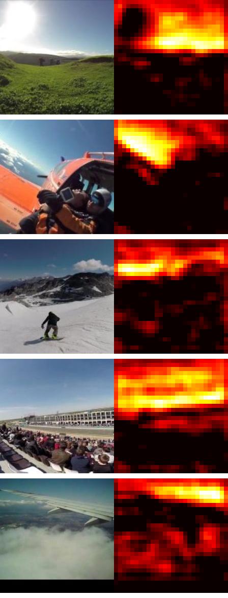
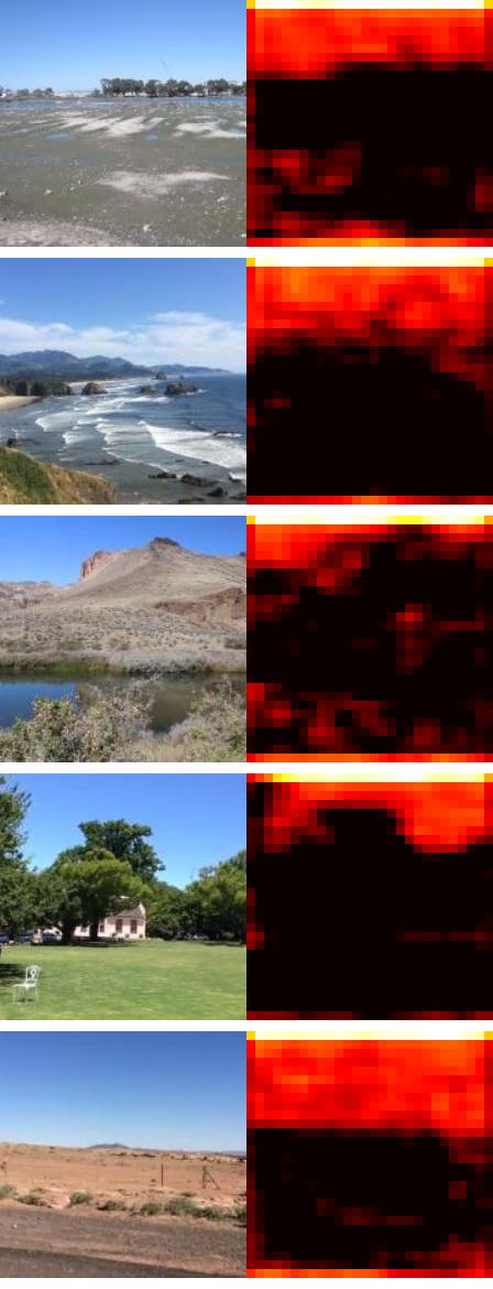
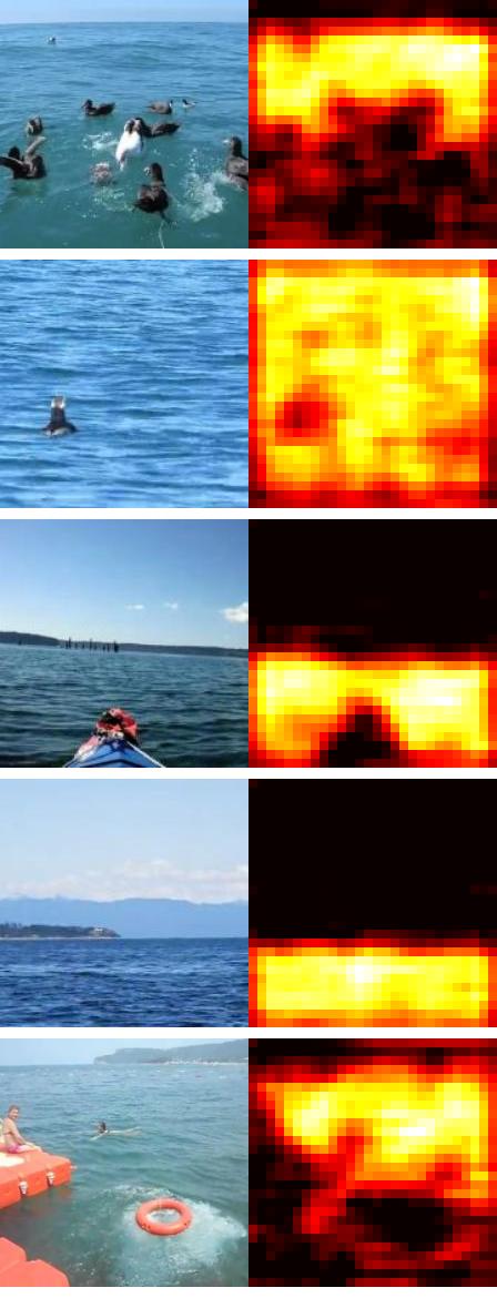
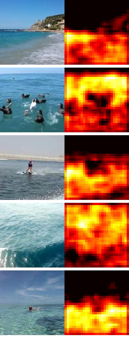
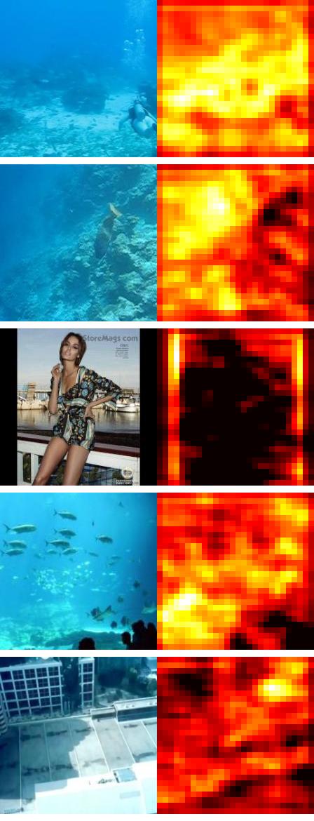
Horizon	Railway	Crowd		Text

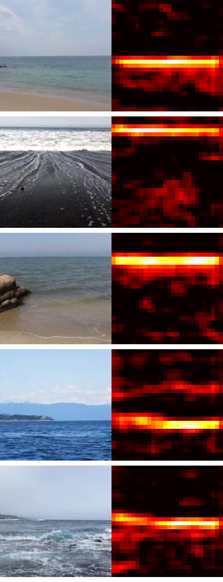
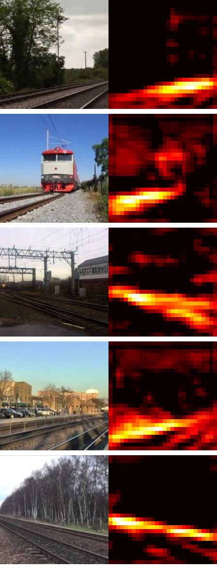
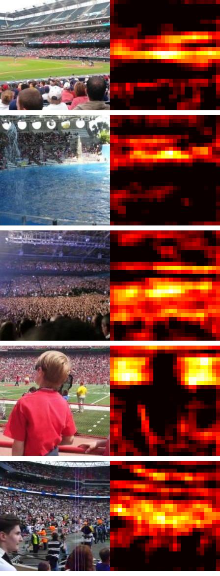
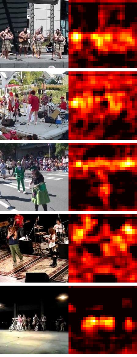
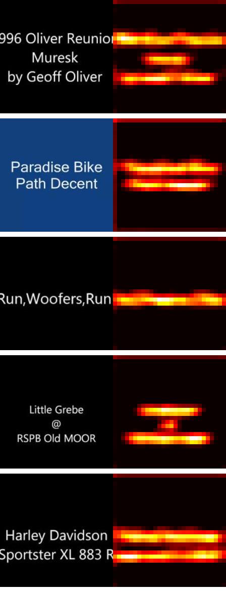
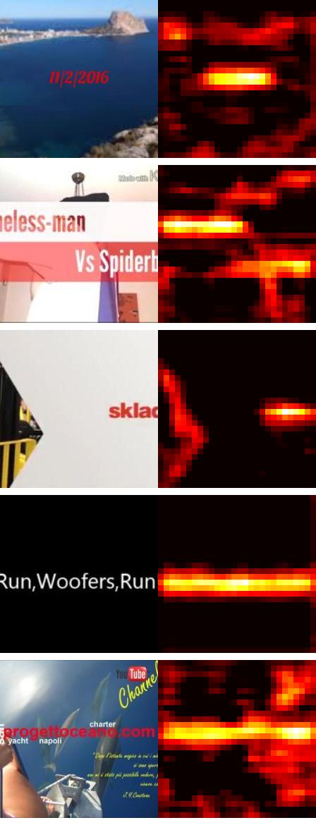
Figure 5: Learnt visual concepts and semantic heatmaps (Flickr-SoundNet). Each mini-column shows five images that most activate a particular unit of the 512 in pool4 of the vision subnetwork, and the corresponding heatmap (for more details see Figures 3 and 4). Column titles are a subjective names of concepts the units respond to.

3.5.2 Audio features

Figure 7 shows what particular audio units are sensitive to in the Kinetics-Sounds dataset. For visualization purposes, instead of showing the sound form, we display the video frame that corresponds to the sound. It can be seen that the audio subnetwork, again without any supervision, manages to learn various semantic entities, as well as perform fine-grained classification (“fingerpicking” vs “playing bass guitar”). Note that some units are naturally confused – the “tap dancing” unit also responds to “pen tapping”, while the “saxophone” unit is sometimes confused with a “trombone”. These are reasonable mistakes, especially when taking into account that the sound input is only one second in length. The audio concepts learnt on the Flickr-SoundNet dataset (Figure 8) follow the same pattern as the visual ones – the network learns to distinguish various scene categories such as water, underwater, outdoors and windy scenes, as well as human-related concepts like baby and human voices, crowds, etc.

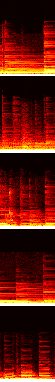
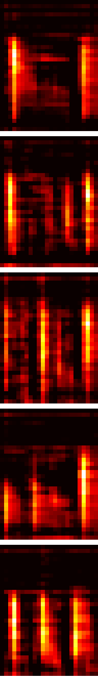
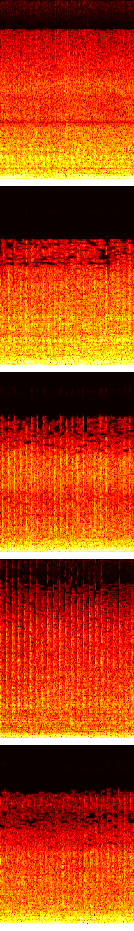
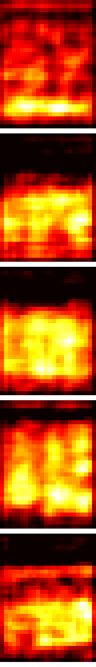
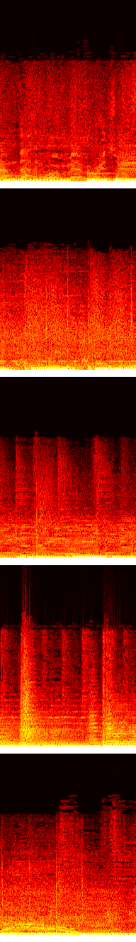
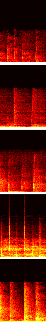
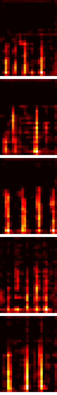
Figure 9: Audio semantic heatmaps (Kinetics-Sounds). Each pair of columns shows a single action class (top, “P.” stands for “playing”), five log-spectrograms (left) and spectrogram semantic heatmaps (right) for the class. Horizontal and vertical axes correspond to the time and frequency dimensions, respectively. A semantic heatmap is obtained as a slice of activations of the unit from conv4_2 of the audio subnetwork which shows preference for the considered class.

Figure 9 shows spectrograms and their semantic heatmaps, illustrating that our $L^{3}$-Net learns to detect audio events. For example, it shows clear preference for low frequencies when detecting bass guitars, attention to wide frequency range when detecting lawnmowers, and temporal ‘steps’ when detecting fingerpicking and tap dancing.

Baby	Face	Head		Crowd

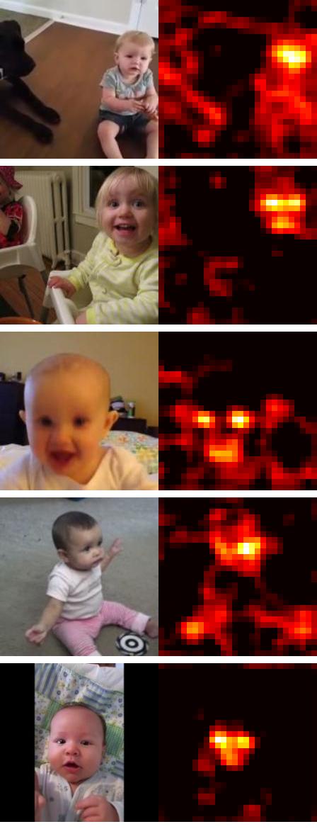
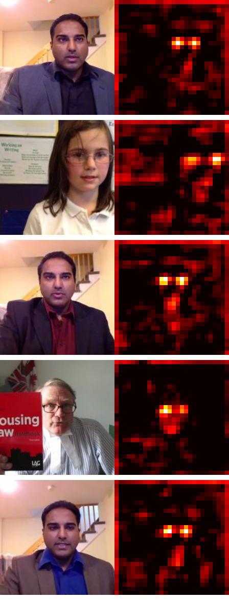
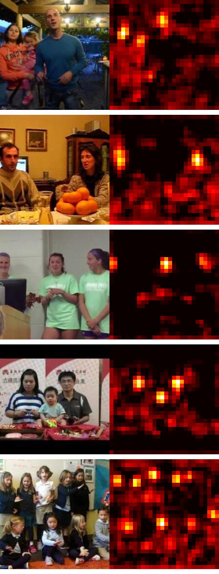
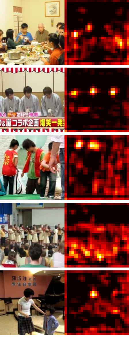
Figure 6: Learnt human-related visual concepts and semantic heatmaps (Flickr-SoundNet). Each mini-column shows five images that most activate a particular unit of the 512 in pool4 of the vision subnetwork, and the corresponding heatmap (for more details see Figures 3 and 4). Column titles are a subjective names of concepts the units respond to.

Fingerpicking	Lawn mowing	P. accordion	P. bass guitar	P. saxophone	Typing	P. xylophone	Tap dancing	Tickling

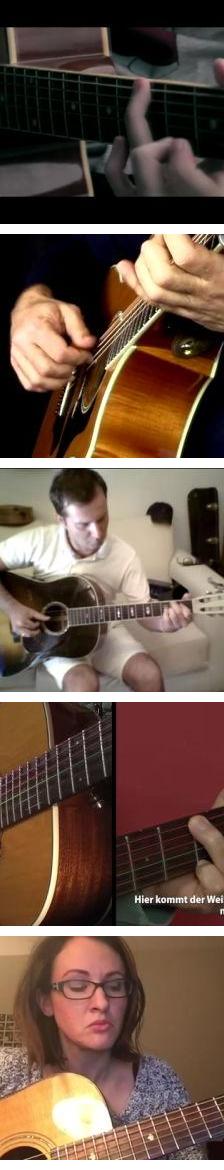
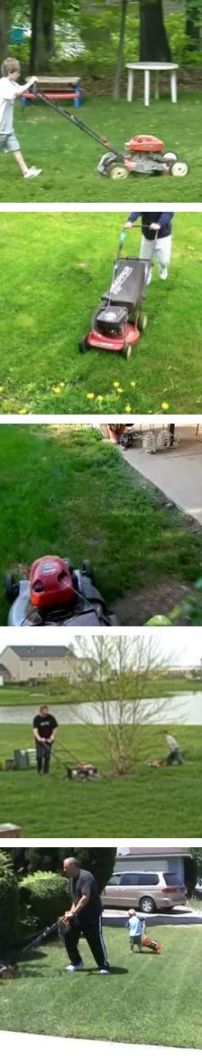
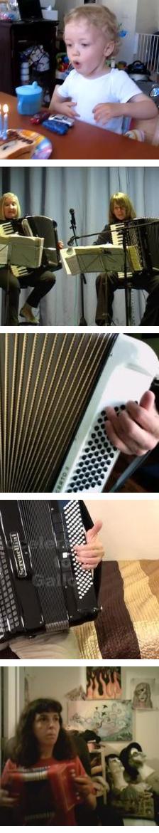
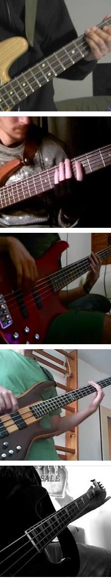
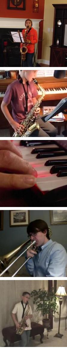
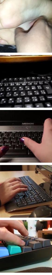
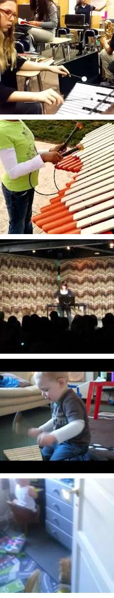
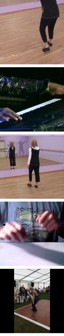
Figure 7: Learnt audio concepts (Kinetics-Sounds). Each column shows five sounds that most activate a particular unit in pool4 of the audio subnetwork. Purely for visualization purposes, as it is hard to display sound, the frame of the video that is aligned with the sound is shown instead of the actual sound form, but we stress that no vision is used in this experiment. Videos come from the Kinetics-Sounds test set and the network was trained on the Kinetics-Sounds train set. The top row shows the dominant action label for the unit (“P.” stands for “playing”).

Baby voice		Human voice		Male voice	People	Crowd
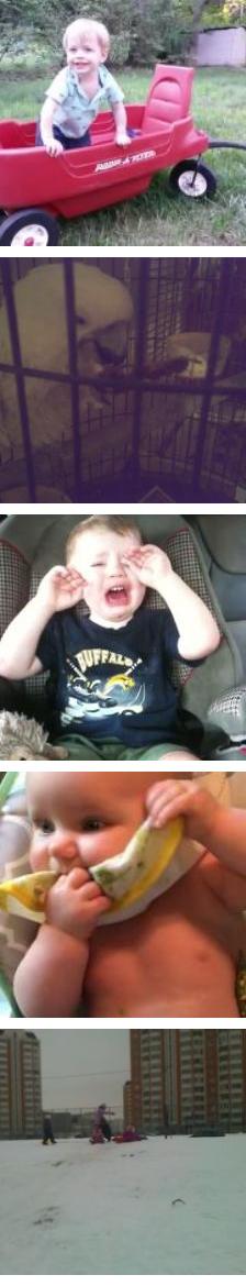
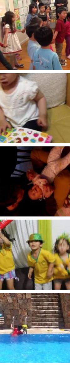
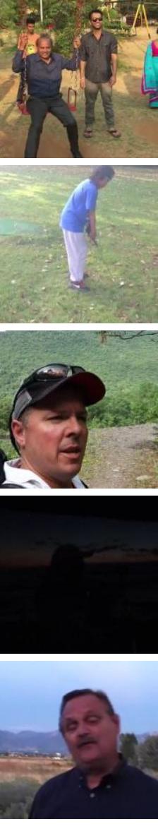
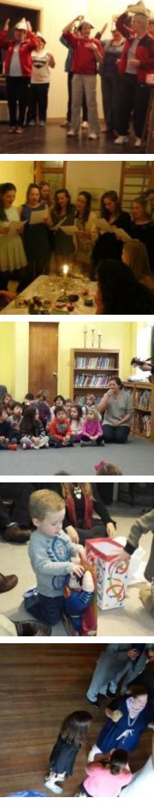
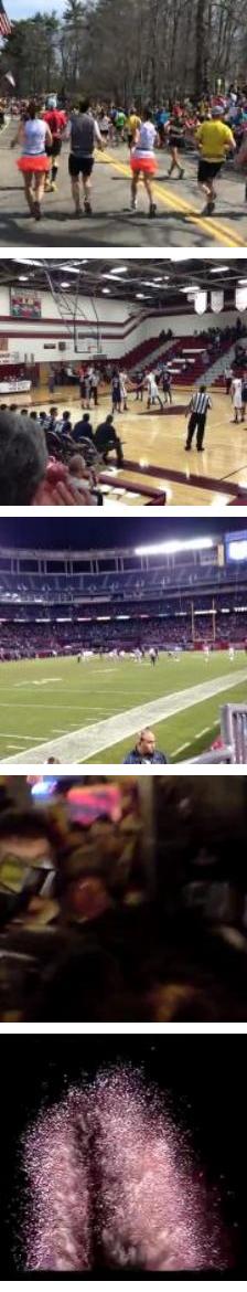
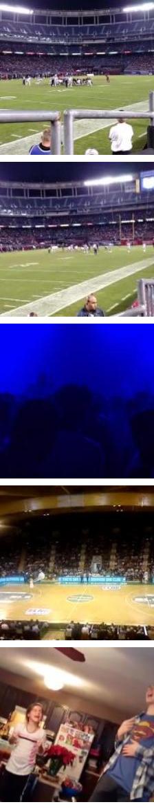
Music	Concert	Sport	Clapping	Water	Underwater	Windy	Outdoor

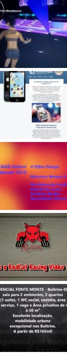
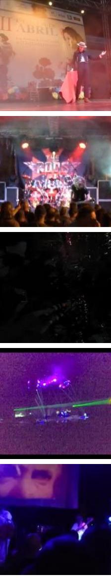
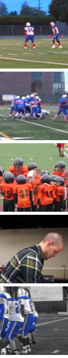
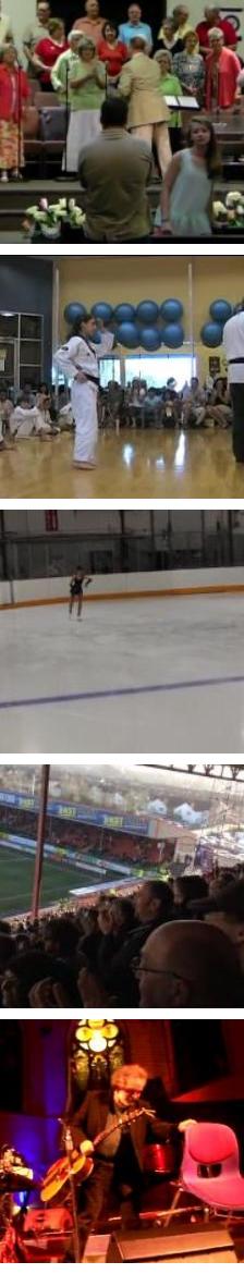
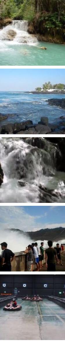
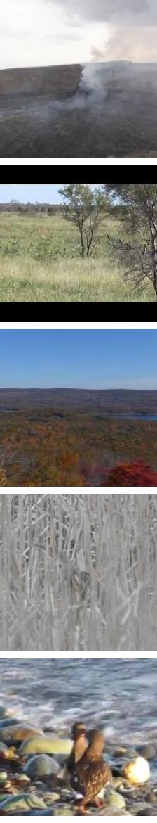
Figure 8: Learnt audio concepts (Flickr-SoundNet). Each mini-column shows sounds that most activate a particular unit of the 512 in pool4 of the audio subnetwork. Purely for visualization purposes, as it is hard to display sound, the frame of the video that is aligned with the sound is shown instead of the actual sound form, but we stress that no vision is used in this experiment. Column titles are a subjective names of concepts the units respond to. Note that for the “Human voice”, “Male voice”, “Crowd”, “Music” and “Concert” examples, the respective clips do contain the relevant audio despite the frame looking as if it is unrelated, e.g. the third example in the “Concert” column does contain loud music sounds. Audio clips containing the five concatenated 1s samples corresponding to each mini-column are hosted on YouTube and can be reached by clicking on the respective mini-columns; this YouTube playlist (https://goo.gl/ohDGtJ) contains all 16 examples.

3.5.3 Versus random features

Could the results in Figures 3, 4, 5, 6, 7 8, and 9 simply be obtained by chance due to examining a large number of units, as colourfully illustrated by the dead salmon experiment [3]? It is unlikely as there are only 512 units in pool4 to choose from, and many of those were found to be highly correlated with a semantic concept. Nevertheless, we repeated the same experiment with a random network (i.e. a network that has not been trained), and have failed to find such correlation. In more detail, we examined how many out of the action classes in Kinetics-Sounds have a unit in pool4 which shows high preference for the class. For the vision subnetwork the preference is determined by ranking all images by their unit activation, and retaining the top 5; if 4 out of these 5 images correspond to one class, then that class is deemed to have a high-preference for the unit (a similar procedure is carried out for the audio subnetwork using spectrograms). Our trained vision and audio networks have high-preference units for 10 and 11 out of a possible 34 action classes, respectively, compared to 1 and 1 for the random vision and audio networks. Furthermore, if the threshold for deeming a unit to be high-preference is reduced to 3, our trained vision and audio subnetworks cover 23 and 20 classes, respectively, compared to the 4 and 3 of a random network, respectively. These results confirm that our network has indeed learnt semantic features.

Furthermore, Figure 10 shows the comparison between the trained and the non-trained (i.e. network with random weights) $L^{3}$-Net representations for the visual and the audio modalities, on the Kinetics-Sounds dataset, using the t-SNE visualization [34]. It is clear that training for the audio-visual correspondence task produces representations that have a semantic meaning, as videos containing the same action classes often cluster together, while the random network’s representations do not exhibit any clustering. There is still a fair amount of confusion in the representations, but this is expected as no class-level supervision is provided and classes can be very alike. For example, an organ and a piano are quite visually similar as they contain keyboards, and the visual difference between a bass guitar and an acoustic guitar is also quite fine; these similarities are reflected in the closeness or overlap of respective clusters in Figure 10(c) (e.g. as noted earlier, “fingerpicking” is mostly associated with acoustic guitars).

Method	Vision	Audio
Random assignments	0.165	0.165
Ours random ($L^{3}$-Net without training)	0.204	0.219
Ours ($L^{3}$-Net self-supervised training)	0.409	0.330

Table 4: Clustering quality. Normalized Mutual Information (NMI) score between the unsupervised clusterings of feature embeddings and the Kinetics-Sounds labels.

We also evaluate the quality of the $L^{3}$-Net embeddings by clustering them with k-means into 64 clusters and reporting the Normalized Mutual Information (NMI) score between the clusters and the ground truth action classes. Results in Table 4 confirm the emergence of semantics as the $L^{3}$-Net embeddings outperform the best random baselines by 50-100%.

The t-SNE visualization also shows some interesting features, such as the “typing” class being divided into two clusters in the visual domain. Further investigation reveals that all frames in one cluster show both a keyboard and hands, while the second cluster contains much fewer hands. Separating these two cases can be a good indication of whether the typing action is happening at the moment captured by the (frame, 1 second sound clip) pair, and thus whether the typing sound is expected to be heard. Furthermore, we found that the “typing” audio samples appear in three clusters – the two fairly pure clusters (outlined in Figure 10(a)) correspond to strong typing sounds and talking while typing, respectively, and the remaining cluster, which is very impure and intermingled with other action classes, mostly corresponds to silence and background noise.

Fingerpicking		Lawn mowing		P. bass guitar		Tap dancing

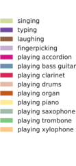
(a) Audio Learnt		(b) Audio Random
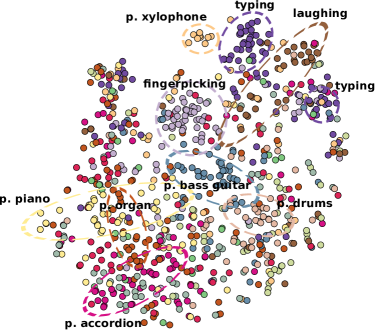
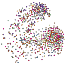
(c) Visual Learnt		(d) Visual Random

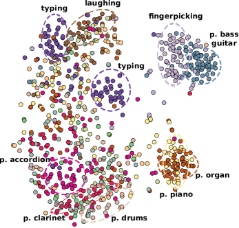
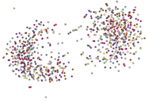
Figure 10: t-SNE visualization [34] of learnt representations (Kinetics-Sounds). The (a,c) and (b,d) show the two-dimensional t-SNE embeddings for the trained versus non-trained (i.e. network with random weights) $L^{3}$-Net, respectively. For visualization purposes only, we colour the t-SNE embeddings using the Kinetics-Sounds labels, but no labels were used for training the $L^{3}$-Net. For clarity and reduced clutter, only a subset of actions (13 classes out of 34) is shown. Some clearly noticeable clusters are manually highlighted by enclosing them with ellipses. Best viewed in colour.

4 Discussion

We have shown that the network trained for the AVC task achieves superior results on sound classification to recent methods that pre-train and fix the visual networks (one each for ImageNet and Scenes), and we conjecture that the reason for this is that the additional freedom of the visual network allows the learning to better take advantage of the opportunities offered by the variety of visual information in the video (rather than be restricted to seeing only through the eyes of the pre-trained network). Also, the visual features that emerge from the $L^{3}$-Net are on par with the state-of-the-art among self-supervised approaches. Furthermore, it has been demonstrated that the network automatically learns, in both modalities, fine-grained distinctions such as bass versus acoustic guitar or saxophone versus clarinet.

The localization visualization results are reminiscent of the classic highlighted pixels in [14], except in our case we do not just learn the few pixels that move (concurrent with the sound) but instead are able to learn extended regions corresponding to the instrument.

We motivated this work by considering correlation of video and audio events. However, we believe there is additional information in concurrency of the two streams, as concurrency is stronger than correlation because the events need to be synchronised (of course, if events are concurrent then they will correlate, but not vice versa). Training for concurrency will require video (multiple frames) as input, rather than a single video frame, but it would be interesting to explore what more is gained from this stronger condition.

In the future, it would be interesting to learn from the recently released large dataset of videos curated according to audio, rather than visual, events [10] and see what subtle visual semantic categories are discovered.

Appendix A Kinetics-Sounds

The 34 action classes taken from the Kinetics dataset [13] to form the Kinetics-Sounds dataset 3.1 are: blowing nose, bowling, chopping wood, ripping paper, shuffling cards, singing, tapping pen, typing, blowing out, dribbling ball, laughing, mowing the lawn by pushing lawnmower, shoveling snow, stomping, tap dancing, tapping guitar, tickling, fingerpicking, patting, playing accordion, playing bagpipes, playing bass guitar, playing clarinet, playing drums, playing guitar, playing harmonica, playing keyboard, playing organ, playing piano, playing saxophone, playing trombone, playing trumpet, playing violin, playing xylophone.

References

- [1] P. Agrawal, J. Carreira, and J. Malik. Learning to see by moving. In Proc. ICCV, 2015.
- [2] Y. Aytar, C. Vondrick, and A. Torralba. SoundNet: Learning sound representations from unlabeled video. In NIPS, 2016.
- [3] C. M. Bennett, M. B. Miller, and G. L. Wolford. Neural correlates of interspecies perspective taking in the post-mortem Atlantic salmon: An argument for multiple comparisons correction. NeuroImage, 2009.
- [4] A. Blum and T. Mitchell. Combining labeled and unlabeled data with co-training. In Computational learning theory, 1998.
- [5] J. S. Chung and A. Zisserman. Out of time: Automated lip sync in the wild. In Workshop on Multi-view Lip-reading, ACCV, 2016.
- [6] C. Doersch, A. Gupta, and A. A. Efros. Unsupervised visual representation learning by context prediction. In Proc. CVPR, 2015.
- [7] J. Donahue, P. Krähenbühl, and T. Darrell. Adversarial feature learning. In Proc. ICLR, 2017.
- [8] A. Dosovitskiy, J. T. Springenberg, M. Riedmiller, and T. Brox. Discriminative unsupervised feature learning with convolutional neural networks. In NIPS, 2014.
- [9] A. Frome, G. S. Corrado, J. Shlens, S. Bengio, J. Dean, M. A. Ranzato, and T. Mikolov. Devise: A deep visual-semantic embedding model. In NIPS, 2013.
- [10] J. F. Gemmeke, D. P. W. Ellis, D. Freedman, A. Jansen, W. Lawrence, R. C. Moore, M. Plakal, and M. Ritter. Audio Set: An ontology and human-labeled dataset for audio events. In ICASSP, 2017.
- [11] D. Harwath, A. Torralba, and J. R. Glass. Unsupervised learning of spoken language with visual context. In NIPS, 2016.
- [12] S. Ioffe and C. Szegedy. Batch normalization: Accelerating deep network training by reducing internal covariate shift. In Proc. ICML, 2015.
- [13] W. Kay, J. Carreira, K. Simonyan, B. Zhang, C. Hillier, S. Vijayanarasimhan, F. Viola, T. Green, T. Back, P. Natsev, M. Suleyman, and A. Zisserman. The Kinetics human action video dataset. CoRR, abs/1705.06950, 2017.
- [14] E. Kidron, Y. Y. Schechner, and M. Elad. Pixels that sound. In Proc. CVPR, 2005.
- [15] D. P. Kingma and J. Ba. Adam: A method for stochastic optimization. In Proc. ICLR, 2015.
- [16] P. Krähenbühl, C. Doersch, J. Donahue, and T. Darrell. Data-dependent initializations of convolutional neural networks. In Proc. ICLR, 2015.
- [17] A. Krizhevsky, I. Sutskever, and G. E. Hinton. ImageNet classification with deep convolutional neural networks. In NIPS, pages 1106–1114, 2012.
- [18] J. Lei Ba, K. Swersky, S. Fidler, and R. Salakhutdinov. Predicting deep zero-shot convolutional neural networks using textual descriptions. In Proc. ICCV, 2015.
- [19] D. Li, J. Tam, and D. Toub. Auditory scene classification using machine learning techniques. IEEE AASP Challenge on Detection and Classification of Acoustic Scenes and Events, 2013.
- [20] I. Misra, C. L. Zitnick, and M. Herbert. Shuffle and learn: Unsupervised learning using temporal order verification. In Proc. ECCV, 2016.
- [21] M. Noroozi and P. Favaro. Unsupervised learning of visual representations by solving jigsaw puzzles. In Proc. ECCV, 2016.
- [22] A. Owens, P. Isola, J. McDermott, A. Torralba, E. Adelson, and W. Freeman. Visually indicated sounds. In Proc. CVPR, 2016.
- [23] A. Owens, W. Jiajun, J. McDermott, W. Freeman, and A. Torralba. Ambient sound provides supervision for visual learning. In Proc. ECCV, 2016.
- [24] D. Pathak, P. Krähenbühl, J. Donahue, T. Darrell, and A. A. Efros. Context encoders: Feature learning by inpainting. In Proc. CVPR, 2016.
- [25] K. J. Piczak. Environmental sound classification with convolutional neural networks. In IEEE Workshop on Machine Learning for Signal processing, 2015.
- [26] K. J. Piczak. ESC: Dataset for environmental sound classification. In Proc. ACMM, 2015.
- [27] A. Rakotomamonjy and G. Gasso. Histogram of gradients of time-frequency representations for audio scene classification. IEEE/ACM Transactions on Audio, Speech, and Language Processing, 2015.
- [28] G. Roma, W. Nogueira, and P. Herrera. Recurrence quantification analysis features for environmental sound recognition. In IEEE Workshop on Applications of Signal Processing to Audio and Acoustics (WASPAA), 2013.
- [29] O. Russakovsky, J. Deng, H. Su, J. Krause, S. Satheesh, S. Ma, S. Huang, A. Karpathy, A. Khosla, M. Bernstein, A. Berg, and F. Li. Imagenet large scale visual recognition challenge. IJCV, 2015.
- [30] K. Simonyan and A. Zisserman. Very deep convolutional networks for large-scale image recognition. In Proc. ICLR, 2015.
- [31] R. Socher, M. Ganjoo, C. D. Manning, and A. Ng. Zero-shot learning through cross-modal transfer. In NIPS, 2013.
- [32] D. Stowell, D. Giannoulis, E. Benetos, M. Lagrange, and M. D. Plumbley. Detection and classification of acoustic scenes and events. In IEEE Transactions on Multimedia, 2015.
- [33] C. Szegedy, V. Vanhoucke, S. Ioffe, J. Shlens, and Z. Wojna. Rethinking the Inception architecture for computer vision. In Proc. CVPR, 2016.
- [34] L. Van der Maaten and G. Hinton. Visualizing data using t-SNE. Journal of Machine Learning Research, 2008.
- [35] X. Wang and A. Gupta. Unsupervised learning of visual representations using videos. In Proc. ICCV, 2015.
- [36] R. Zhang, P. Isola, and A. A. Efros. Colorful image colorization. In Proc. ECCV, 2016.