Combinatorial Semi-Bandits with Knapsacks††thanks: Extended abstract appears in the 21st International Conference on Artificial Intelligence and Statistics (AIStats 2018).
Abstract
We unify two prominent lines of work on multi-armed bandits: bandits with knapsacks and combinatorial semi-bandits. The former concerns limited “resources” consumed by the algorithm, e.g., limited supply in dynamic pricing. The latter allows a huge number of actions but assumes combinatorial structure and additional feedback to make the problem tractable. We define a common generalization, support it with several motivating examples, and design an algorithm for it. Our regret bounds are comparable with those for and combinatorial semi-bandits.
1 Introduction
Multi-armed bandits (MAB) is an elegant model for studying the tradeoff between acquisition and usage of information, a.k.a. explore-exploit tradeoff (Robbins, 1952; Thompson, 1933). In each round an algorithm sequentially chooses from a fixed set of alternatives (sometimes known as actions or arms), and receives reward for the chosen action. Crucially, the algorithm does not have enough information to answer all “counterfactual” questions about what would have happened if a different action was chosen in this round. MAB problems have been studied steadily since 1930-ies, with a huge surge of interest in the last decade.
This paper combines two lines of work related to bandits: on bandits with knapsacks () (Badanidiyuru et al., 2013a) and on combinatorial semi-bandits (György et al., 2007). concern scenarios with limited “resources” consumed by the algorithm, e.g., limited inventory in a dynamic pricing problem. In combinatorial semi-bandits, actions correspond to subsets of some “ground set”, rewards are additive across the elements of this ground set (atoms), and the reward for each chosen atom is revealed (semi-bandit feedback). A paradigmatic example is an online routing problem, where atoms are edges in a graph, and actions are paths. Both lines of work have received much recent attention and are supported by numerous examples.
Our contributions. We define a common generalization of combinatorial semi-bandits and , termed Combinatorial Semi-Bandits with Knapsacks (). Following all prior work on , we focus on an i.i.d. environment: in each round, the “outcome” is drawn independently from a fixed distribution over the possible outcomes. Here the “outcome” of a round is the matrix of reward and resource consumption for all atoms.111Our model allows arbitrary correlations within a given round, both across rewards and consumption for the same atom and across multiple atoms. Such correlations are essential in applications such as dynamic pricing and dynamic assortment. E.g., customers’ valuations can be correlated across products, and algorithm earns only if it sells; see Section 5 for details. We design an algorithm for , achieving regret rates that are comparable with those for and combinatorial semi-bandits.
Specifics are as follows. As usual, we assume “bounded outcomes”: for each atom and each round, rewards and consumption of each resource is non-negative and at most . Regret is relative to the expected total reward of the best all-knowing policy, denoted . For problems, this is known to be a much stronger benchmark than the traditional best-fixed-arm benchmark. We upper-bound the regret in terms of the relevant parameters: time horizon , (smallest) budget , number of atoms , and itself (which may be as large as ). We obtain
| (1.1) |
The “shape” of the regret bound is consistent with prior work: the additive term appears in the optimal regret bound for , and the and additive terms are very common in regret bounds for MAB. The per-round running time is polynomial in , and near-linear in for some important special cases.
Our regret bound is optimal up to factors for paradigmatic special cases. is a special case when actions are atoms. For , the regret bound becomes , where is the number of actions, which coincides with the lower bound from (Badanidiyuru et al., 2013a). Combinatorial semi-bandits is a special case with . If all feasible subsets contain at most atoms, we have , and the regret bound becomes . This coincides with the lower bound from (Kveton et al., 2014).
Our main result assumes that the action set, i.e., the family of feasible subsets of atoms, is described by a matroid constraint.222Matroid is a standard notion in combinatorial optimization which abstracts and generalizes linear independence. This is a rather general scenario which includes many paradigmatic special cases of combinatorial semi-bandits such as cardinality constraints, partition matroid constraints, and spanning tree constraints. We also assume that .
Our model captures several application scenarios, incl. dynamic pricing, dynamic assortment, repeated auctions, and repeated bidding. We work out these applications, and explain how our regret bounds improve over prior work.
Challenges and techniques. problems are challenging compared to traditional MAB problems with i.i.d. rewards because it no longer suffices to look for the best action and/or optimize expected per-round rewards; instead, one essentially needs to look for a distribution over actions with optimal expected total reward across all rounds. Generic challenges in combinatorial semi-bandits concern handling exponentially many actions (both in terms of regret and in terms of the running time), and taking advantage of the additional feedback. And in , one needs to deal with distributions over subsets of atoms, rather than “just” with distributions over actions.
Our algorithm connects a technique from and a randomized rounding technique from combinatorial optimization. (With five existing algorithms and a wealth of approaches for combinatorial optimization, choosing the techniques is a part of the challenge.)
We build on a algorithm from Agrawal and Devanur (2014a), which combines linear relaxations and a well-known ”optimism-under-uncertainty” paradigm. A generalization of this algorithm to results in a fractional solution , a vector over atoms. Randomized rounding converts into a distribution over feasible subsets of atoms that equals in expectation. It is crucial (and challenging) to ensure that this distribution contains enough randomness so as to admit concentration bounds not only across rounds, but also across atoms. Our analysis ”opens up” a fairly technical proof from prior work and intertwines it with a new argument based on negative correlation.
We present our algorithm and analysis so as to ”plug in” any suitable randomized rounding technique. This makes our presentation more lucid, and also leads to faster running times for important special cases.
Solving using prior work. Solving using an algorithm for would result in a regret bound like (1.1) with replaced with the number of actions. The latter could be on the order of if each action can consist of at most atoms, or perhaps even exponential in .
can be solved as a special case of a much more general linear-contextual extension of from Agrawal and Devanur (2014a, 2016). In their model, an algorithm takes advantage of the combinatorial structure of actions, yet it ignores the additional feedback from the atoms. Their regret bounds have a worse dependence on the parameters, and apply for a much more limited range of parameters. Further, their per-round running time is linear in the number of actions, which is often prohibitively large.
To compare the regret bounds, let us focus on instances of in which at most one unit of each resource is consumed in each round. (This is the case in all our motivating applications, except repeated bidding.) Then Agrawal and Devanur (2014a, 2016) assume , and achieve regret . 333Agrawal and Devanur (2014a, 2016) state regret bound with term rather than , but they assume that per-round rewards lie in . Since per-round rewards can be as large as in our setting, we need to scale down all rewards by a factor of , apply their regret bound, and then scale back, which results in the regret bound with . When per-round consumption can be as large as , regret bound from Agrawal and Devanur (2014a, 2016) becomes due to rescaling. It is easy to see that we improve upon the range and upon both summands. In particular, we improve both summands by the factor of in a lucid special case when and .444 In prior work on combinatorial bandits (without constraints), semi-bandit feedback improves regret bound by a factor of , see the discussion in Kveton et al. (2015b).
We run simulations to compare our algorithm against prior work on and combinatorial semi-bandits.
Related work. Multi-armed bandits have been studied since Thompson (1933) in Operations Research, Economics, and several branches of Computer Science, see (Gittins et al., 2011; Bubeck and Cesa-Bianchi, 2012) for background. Among broad directions in MAB, most relevant is MAB with i.i.d. rewards, starting from (Lai and Robbins, 1985; Auer et al., 2002).
Bandits with Knapsacks () were first introduced by Badanidiyuru et al. (2013a) as a common generalization of several models from prior work and many other motivating examples. Subsequent papers extended to “smoother” resource constraints and introduced several new algorithms (Agrawal and Devanur, 2014a), and generalized to contextual bandits (Badanidiyuru et al., 2014; Agrawal et al., 2016; Agrawal and Devanur, 2016). All prior work on and special cases thereof assumed i.i.d. outcomes.
Special cases of include dynamic pricing with limited supply (Babaioff et al., 2015; Besbes and Zeevi, 2009, 2012; Wang et al., 2014), dynamic procurement on a budget (Badanidiyuru et al., 2012; Singla and Krause, 2013; Slivkins and Vaughan, 2013), dynamic ad allocation with advertiser budgets (Slivkins, 2013), and bandits with a single deterministic resource (Guha and Munagala, 2007; Gupta et al., 2011; Tran-Thanh et al., 2010, 2012). Some special cases admit instance-dependent logarithmic regret bounds (Xia et al., 2016b, a; Combes et al., 2015a; Slivkins, 2013) when there is only one bounded resource and unbounded time, or when resource constraints do not bind across arms.
Combinatorial semi-bandits were studied by György et al. (2007), in the adversarial setting. In the i.i.d. setting, in a series of works by (Anantharam et al., 1987; Gai et al., 2010, 2012; Chen et al., 2013; Kveton et al., 2015b; Combes et al., 2015b), an optimal algorithm was achieved. This result was then extended to atoms with linear rewards by Wen et al. (2015). Kveton et al. (2014) obtained improved results for the special case when action set is described by a matroid. Some other works studied a closely related “cascade model”, where the ordering of atoms matters (Kveton et al., 2015a; Katariya et al., 2016; Zong et al., 2016). Contextual semi-bandits have been studied in (Wen et al., 2015; Krishnamurthy et al., 2016).
Randomized rounding schemes (RRS) come from the literature on approximation algorithms in combinatorial optimization (see Williamson and Shmoys (2011); Papadimitriou and Steiglitz (1982) for background). RRS were introduced in Raghavan and Tompson (1987). Subsequent work (Gandhi et al., 2006; Asadpour et al., 2010; Chekuri et al., 2010, 2011) developed RRS which correlate the rounded random variables so as to guarantee sharp concentration bounds.
Discussion. The basic model of multi-armed bandits can be extended in many distinct directions: what auxiliary information, if any, is revealed to the algorithm before it needs to make a decision, which feedback is revealed afterwards, which “process” are the rewards coming from, do they have some known structure that can be leveraged, are there global constraints on the algorithm, etc. While many real-life scenarios combine several directions, most existing work proceeds along only one or two. We believe it is important (and often quite challenging) to unify these lines of work. For example, an important recent result of Syrgkanis et al. (2016); Rakhlin and Sridharan (2016) combined “contextual” and “adversarial” bandits.
2 Our model and preliminaries
Our model, called Semi-Bandits with Knapsacks () is a generalization of multi-armed bandits (henceforth, MAB) with i.i.d. rewards. As such, in each round , an algorithm chooses an action from a fixed set of actions , and receives a reward for this action which is drawn independently from a fixed distribution that depends only on the chosen action. The number of rounds , a.k.a. the time horizon, is known.
There are resources being consumed by the algorithm. The algorithm starts out with budget of each resource . All budgets are known to the algorithm. If in round action is chosen, the outcome of this round is not only the reward but the consumption of each resource . We refer to as the consumption vector.555We use bold font to indicate vectors and matrices. Following prior work on , we assume that all budgets are the same: for all resources .666This is w.l.o.g. because we can divide all consumption of each resource by . Effectively, is the smallest budget in the original problem instance. Algorithm stops as soon as any one of the resources goes strictly below 0. The round in which this happens is called the stopping time and denoted . The reward collected in this last round does not count; so the total reward of the algorithm is .
Actions correspond to subsets of a finite ground set , with ; we refer to elements of as atoms. Thus, the set of actions corresponds to the family of “feasible subsets” of . The rewards and resource consumption is additive over the atoms: for each round and each atom there is a reward and consumption vector such that for each action it holds that and .
We assume the i.i.d. property across rounds, but allow arbitrary correlations within the same round. Formally, for a given round we consider the “outcome matrix” , which specifies rewards and resource consumption for all resources and all atoms. We assume that the outcome matrix is chosen independently from a fixed distribution over such matrices. The distribution is not revealed to the algorithm. The mean rewards and mean consumption is denoted and . We extend the notation to actions, i.e., to subsets of atoms: and .
An instance of consists of the action set , the budgets , and the distribution . The and are known to the algorithm, and is not. As explained in the introduction, subsumes Bandits with Knapsacks () and semi-bandits. is the special case when consists of singletons, and semi-bandits is the special case when all budgets are equal to (so that the resource consumption is irrelevant).
Following the prior work on , we compete against the “optimal all-knowing algorithm”: an algorithm that optimizes the expected total reward for a given problem instance; its expected total reward is denoted by . As observed in Badanidiyuru et al. (2013a), can be much larger (e.g., factor of 2 larger) than the expected cumulative reward of the best action, for a variety of important special cases of . Our goal is to minimize regret, defined as minus algorithm’s total reward.
Combinatorial constraints. Action set is given by a combinatorial constraint, i.e., a family of subsets. Treating subsets of atoms as -dimensional binary vectors, corresponds to a finite set of points in . We assume that the convex hull of forms a polytope in . In other words, there exists a set of linear constraints over whose set of feasible integral solutions is . We call such linearizable; the convex hull is called the polytope induced by .
Our main result is for matroid constraints, a family of linearizable combinatorial constraints which subsumes several important special cases such as cardinality constraints, partition matroid constraints, spanning tree constraints and transversal constraints. Formally, is a matroid if it contains the empty set, and satisfies two properties: (i) if contains a subset , then it also contains every subset of , and (ii) for any two subsets with it holds that for each atom . See Appendix B for more background and examples.
We incorporate prior work on randomized rounding for linear programs. Consider a linearizable action set with induced polytope . The randomized rounding scheme (henceforth, ) for is an algorithm which inputs a feasible fractional solution and the linear equations describing , and produces a random vector over . We consider ’s such that and is negatively correlated (see below for definition); we call such ’s negatively correlated. Several such are known: e.g., for cardinality constraints and bipartite matching (Gandhi et al., 2006), for spanning trees (Asadpour et al., 2010), and for matroids (Chekuri et al., 2010).
Negative correlation. Let denote a family of random variables which take values in . Let be the average, and .
Family is called negatively correlated if
| (2.1) | |||
| (2.2) |
Independent random variables satisfy both properties with equality. For intuition: if are Bernoulli and (2.1) is strict, then is more likely to be if .
Negative correlation is a generalization of independence that allows for similar concentration bounds, i.e., high-probability upper bounds on . However, our analysis does not invoke them directly. Instead, we use a concentration bound given a closely related property:
| (2.3) |
Theorem 2.1.
If (2.3), then for some absolute constant ,
| (2.4) |
Confidence radius. We bound deviations in a way that gets sharper when is small, without knowing in advance. (We use the notation as above.) To this end, we use the notion of confidence radius from (Kleinberg et al., 2015; Babaioff et al., 2015; Badanidiyuru et al., 2013a; Agrawal and Devanur, 2014b)777For instance Theorem 2.1 in (Badanidiyuru et al., 2013b):
| (2.5) |
If random variables are independent, then event
| (2.6) |
happens with probability at least , for any given . We use this notion to define upper/lower confidence bounds on the mean rewards and mean resource consumption. Fix round , atom , and resource . Let and denote the empirical average of the rewards and resource- consumption, resp., between rounds and . Let be the number of times atom has been chosen in these rounds (i.e., included in the chosen actions). The confidence bounds are defined as
| (2.7) |
where denotes the projection into . We always use the same parameter , for an appropriately chosen absolute constant . We suppress and from the notation. We use a vector notation and to denote the corresponding -dimensional vectors over all atoms .
By (2.6), with probability the following hold.
3 Main algorithm
Let us define our main algorithm, called . The algorithm builds on an arbitrary for the action set . It is parameterized by this , the polytope induced by (represented as a collection of linear constraints), and a number . In each round , it recomputes the upper/lower confidence bounds, as defined in (2.7), and solves the following linear program:
| () |
This linear program defines a linear relaxation of the original problem which is “optimistic” in the sense that it uses upper confidence bounds for rewards and lower confidence bounds for consumption. The linear relaxation is also “conservative” in the sense that it rescales the budget by . Essentially, this is to ensure that the algorithm does not run out of budget with high probability. Parameter will be fixed throughout. For ease of notation, we will denote henceforth. The LP solution can be seen as a probability vector over the atoms. Finally, the algorithm uses the to convert the LP solution into a feasible action. The pseudocode is given as Algorithm 1.
-
1.
Recompute Confidence Bounds as in (2.7)
Obtain a feasible action by invoking the on vector .
Semi-bandit Feedback: observe the rewards/consumption for all atoms .
If action set is described by a matroid constraint, we can use the negatively correlated from Chekuri et al. (2010). In particular, we obtain a complete algorithm for several combinatorial constraints commonly used in the literature on semi-bandits, such as partition matroid constraints, spanning trees. More background on matroid constraints can be found in the Appendix B.
Theorem 3.1.
Consider the problem with a linearizable action set that admits a negatively correlated . Then algorithm with this achieves expected regret bound at most
| (3.1) |
Here is the time horizon, is the number of atoms, and is the budget. We require , where is the parameter in confidence radius. Parameter in the algorithm is set to .
Corollary 3.2.
Running time of the algorithm. The algorithm does two computationally intensive steps in each round: solves the linear program () and runs the . For matroid constraints, the from Chekuri et al. (2010) has running time. Hence, in the general case the computational bottleneck is solving the LP, which has variables and constraints. Matroids are known to admit a polynomial-time seperation oracle (e.g., see Schrijver, 2002). It follows that the entire set of constraints in admits a polynomial-time separation oracle, and therefore we can use the Ellipsoid algorithm to solve in polynomial time. For some classes of matroid constraints the LP is much smaller: e.g., for cardinality constraints (just constraints) and for traversal matroids on bipartite graphs (just constraints). Then near-linear-time algorithms can be used.
Our algorithm works under any negatively correlated RRS. We can use this flexibility to improve the per-round running time for some special cases. (Making decisions extremely fast is often critical in practical applications of bandits (e.g., see Agarwal et al., 2016).) We obtain near-linear per-round running times for cardinality constraints and partition matroid constraints. Indeed, can be solved in near-linear time, as mentioned above, and we can use a negatively correlated RRS from (Gandhi et al., 2006) which runs in linear time. These classes of matroid constraints are important in our applications (see Section 5).
4 Proof of Theorem 3.1
Proof overview. First, we argue that provides a good benchmark that we can use instead of . Specifically, at any given round, the optimal value for in each round is at least with high probability. We prove this by constructing a series of LPs, starting with a generic linear relaxation for and ending with , and showing that the optimal value does not decrease along the series.
Next we define an event that occur with high probability, henceforth called clean event. This event concerns total rewards, and compares our algorithm against :
| (4.1) |
We prove that it is indeed a high-probability event in three steps. First, we relate the algorithm’s reward to its expected reward , where we interpret the chosen action , a subset of atoms, as a binary vector over the atoms. Then we relate to , replacing expected rewards with the upper confidence bounds. Finally, we relate to , replacing the output of the RRS with the corresponding expectations. Putting it together, we relate algorithm’s reward to , as needed. It is essential to bound the deviations in the sharpest way possible; in particular, the naive bounds are not good enough. To this end, we use several tools: the confidence radius from (2.5), the negative correlation property of the RRS, and another concentration bound from prior work.
A similar “clean event” (with a similar proof) concerns the total resource consumption of the algorithm. We condition on both clean events, and perform the rest of the analysis via a “deterministic” argument not involving probabilities. In particular, we use the second “clean event” to guarantee that the algorithm never runs out of resources.
We use negative correlation via a rather delicate argument. We extend the concentration bound in Theorem 2.1 to a random process that evolves over time, and only assumes that property (2.3) holds within each round conditional on the history. For a given round, we start with a negative correlation property of and construct another family of random variables that conditionally satisfies (2.3). The extended concentration bound is then applied to this family. The net result is a concentration bound for as if we had independent random variables there.
The rest of the section contains the full proof.
4.1 Linear programs
We argue that provides a good benchmark that we can use instead of . Fix round and let denote the optimal value for in this round. Then:
Lemma 4.1.
with probability at least .
We will prove this by constructing a series of LP’s, starting with a generic linear relaxation for and ending with . We show that along the series the optimal value does not decrease with high probability.
The first LP, adapted from Badanidiyuru et al. (2013a), has one decision variable for each action, and applies generically to any problem.
| () |
Let denote the optimal value of this LP with a given budget . Then:
Claim 4.2.
.
Proof.
The second inequality in Claim 4.2 follows from (Lemma 3.1 in Badanidiyuru et al., 2013a). We will prove the first inequality as follows. Let denote an optimal solution to (B). Consider ; this is feasible to (), since for every ,
Hence, this is a feasible solution. Now, consider the objective function. Let denote an optimal solution to (). We have that
Now consider a simpler LP where the decision variables correspond to atoms. As before, denotes the polytope induced by action set .
| () |
Here is the matrix of expected consumption, and denotes its transpose. The notation means that the inequality holds for for each coordinate.
Claim 4.3.
With probability at least we have, .
Proof.
We will first prove the second inequality.
We will now map this to a feasible solution to and show that the objective value does not decrease. This will then complete the claim. Consider the following solution defined as follows.
We will now show that is a feasible solution to the polytope . From the definition of , we can write it as . Here, is a binary vector, such that it has at position if and only if atom is present in set . Hence, is a point in the polytope since it can be written as convex combination of its vertices.
Now, we will show that, also satisfies the resource consumption constraint.
The last inequality is because in the optimal solution, the x value corresponding to subset is 1 while rest all are 0. We will now show that produces an objective value at least as large as .
Now we will prove the first inequality. We will assume the “clean event” that and for all . Hence, the inequality holds with probability at least .
Consider a time . Given an optimal solution to we will show that this is feasible to . Note that, satisfies the constraint set since that is same for both and . Now consider the constraint . Note that . Hence, we have that . The last inequality is because is a feasible solution to .
Now consider the objective function. Let denote the optimal solution to .
.
∎
4.2 Negative correlation and concentration bounds
Our analysis relies on several facts about negative correlation and concentration bounds. First, we argue that property (2.1) in the definition of negative correlation is preserved under a specific linear transformation:
Claim 4.4.
Suppose is a family of negatively correlated random variables with support . Fix numbers . Consider two families of random variables:
Then both families satisfy property (2.1).
Proof.
Let us focus on family ; the proof for family is very similar.
Denote and and for all . Note that and . Fix a subset . We have,
| by Binomial Theorem | ||||
| (2.1) invariant under non-negative scaling, neg. correlated | ||||
| by Binomial Theorem | ||||
Second, we extend Theorem 2.1 to a random process that evolves over time, and only assumes that property (2.3) holds within each round conditional on the history.
Theorem 4.5.
Let be a family of random variables taking values in . Assume random variables satisfy property (2.1) given and have expectation given , for each round . Let be the average. Then for some absolute constant ,
| (4.2) |
Proof.
We prove that family satisfies property (2.3), and then invoke Theorem 2.1. Let us restate property (2.3) for the sake of completeness:
| (4.3) |
Fix subset . Partition into subsets , for each round . Fix round and denote
We will now prove the following statement by induction on :
| (4.4) |
The base case is when . Note that is just the product of elements in set and they are negatively correlated from the premise. Therefore we are done. Now for the inductive case of ,
| From property (2.1) in the conditional space | (4.5) | ||||
| From assumption in Lemma 4.5 | (4.6) |
Third, we invoke Eq. 2.6 for rewards and resource consumptions:
Lemma 4.6.
With probability at least , we have the following:
| (4.7) | ||||
Fourth, we use a concentration bound from prior work which gets sharper when the expected sum is very small, and does not rely on independent random variables:
Theorem 4.7 (Babaioff et al. (2015)).
Let denote a set of random variables. For each , let denote the multiplier determined by random variables . Let where . Then for any , we have the following with probability at least :
4.3 Analysis of the “clean event”
Let us set up several events, henceforth called clean events, and prove that they hold with high probability. Then the remainder of the analysis can proceed conditional on the intersection of these events. The clean events are similar to the ones in Agrawal and Devanur (2014b), but are somewhat “stronger”, essentially because our algorithm has access to per-atom feedback and our analysis can use the negative correlation property of the .
In what follows, it is convenient to consider a version of in which the algorithm does not stop, so that we can argue about what happens w.h.p. if our algorithm runs for the full rounds. Then we show that our algorithm does indeed run for the full rounds w.h.p.
Recall that be the optimal fractional solution obtained by solving the LP in round . Let be the random binary vector obtained by invoking the (so that the chosen action corresponds to a particular realization of , interpreted as a subset). Let denote the family of RRS realizations up to round .
4.3.1 “Clean event” for rewards
For brevity, for each round let be the vector of realized rewards, and let be the algorithm’s reward at this round.
Lemma 4.8.
Consider without stopping. Then with probability at least :
Proof.
We prove the Lemma by proving the following three high-probability inequalities.
With probability at least : the following holds:
| (4.8) | ||||
| (4.9) | ||||
| (4.10) |
We will use the properties of to prove Eq. 4.10. Proof of Eq. 4.9 is similar to Agrawal and Devanur (2014b), while proof of Eq. 4.8 follows immediately from the setup of the model. Using the parts (4.8) and (4.10) we can now find an appropriate upper bound on and using this upper bound, we prove Lemma 4.8.
Proof of Eq. 4.8. Recall that . Note that, when the expectation is taken over just the independent samples of . By Theorem 4.7, with probability we have:
Proof of Eq. 4.9. For this part, the arguments similar to Agrawal and Devanur (2014b) follow with some minor adaptations. For sake of completeness we describe the full proof. Note that we have,
Now, using Lemma 4.6 in Appendix, we have that with probability
Hence, we have
The last inequality is from the definition of function and using the Cauchy-Swartz inequality. Note that . Also, since we have with probability , , we have,
Finally note that is a feasible solution to the semi-bandit polytope . Hence, we have that
Hence,
Proof of Eq. 4.10: Recall that for each round , the UCB vector is determined by the random variables . Further, conditional on a realization of , the random variables are negatively correlated from the property of RRS. Let , . Note that we have . Define
From Claim 4.4, we have that conditioned on satisfy (2.1). Further, . Therefore, the family satisfies the assumptions in Theorem 4.5 and hence satisfies Eq. 4.2 for some absolute constant . Plugging back the ’s, we obtain an upper-tail concentration bound:
To obtain a corresponding concentration bound for the lower tail, we apply a similar argument to
Once again from Claim 4.4, we have that conditioned on satisfy (2.1). The family satisfies the assumptions in Theorem 4.5 and hence satisfies Eq. 4.2. Plugging back the ’s, we obtain a lower-tail concentration bound:
Combining these two we have,
| (4.11) |
Hence setting , we obtain Eq. 4.10 with probability at least .
Rearranging and solving for , we have
4.3.2 “Clean event” for resource consumption
We define a similar “clean event” for consumption of each resource . By a slight abuse of notation, for each round let be the vector of realized consumption of resource . Let denote algorithm’s consumption for resource at round (i.e., ).
Lemma 4.9.
Consider without stopping. Then with probability at least :
Proof.
The proof is similar to Lemma 4.8. We will split the proof into following three equations. Fix an arbitrary resource . With probability at least the following holds:
| (4.13) |
| (4.14) |
| (4.15) |
Using the parts 4.13, 4.14 and 4.15 we can find an upper bound on . Hence, combining Lemmas 4.13, 4.14 and 4.15 with this bound and taking an Union Bound over all the resources, we get Lemma 4.9.
Proof of Eq. 4.13. We have that is a set of independent random variables over a probability spacee . Note that, . Hence, we can invoke Theorem 4.7 on independent random variables to get with probability
Proof of Eq. 4.14. This is very similar to proof of 4.9 and we will skip the repetitive parts. Hence, we have with probability
Proof of Eq. 4.15. Recall that for each round and each resource , the LCB vector is determined by the random variables . Similar to the proof of Eq. 4.10, random variables obtained from the RRS are negatively correlated given . As before define , . We have that .
By Claim 4.4, random variables
satisfy (2.1), given . We conclude that family satisfies the assumptions in Theorem 4.5, and therefore satisfies Eq. 4.2 for some absolute constant . Therefore, we obtain an upper-tail concentration bound for ’s:
To obtain a corresponding concentration bound for the lower tail, we apply a similar argument to
Once again, invoking Claim 4.4 we have that conditioned on satisfy (2.1). Thus, family satisfies the assumptions in Theorem 4.5, and therefore satisfies Eq. 4.2. We obtain:
Combing the two tails we have,
| (4.16) |
Once again, setting , we obtain Eq. 4.15 with probability at least .
Proof of Lemma 4.9. Denote . From Equation 4.13, 4.14 and 4.15, we have that . Note that . Hence, . Hence, re-arranging this gives us . Plugging this back in Equations 4.13, 4.14 and 4.15, we get Lemma 4.9.
∎
4.4 Putting it all together
Similar to Agrawal and Devanur (2014b), we will handle the hard constraint on budget, by choosing an appropriate value of . We then combine the above Lemma on ”rewards” clean event to compare the reward of the algorithm with that of the optimal value of LP to obtain the regret bound in Theorem 3.1. Additionally, we use the Lemma on ”consumption” clean event to argue that the algorithm doesn’t exhaust the resource budget before round . Formally, consider the following.
Recall that from Lemma 4.1, we have . Let us define the performance of the algorithm as . From Lemma 4.8, that with probability at least
Choosing and using the assumption that , we derive Eq. 3.1. For any given , we set to obtain a success probability of at least .
Now we will argue that the algorithm does not exhaust the resource budget before round with probability at least . Note that for every resource ,
Hence, combining this with Lemma 4.9, we have
5 Applications and special cases
Let us discuss some notable examples of (which generalize some of the numerous applications listed in Badanidiyuru et al. (2013a)). Our results for these examples improve exponentially over a naive application of the framework. Compared to what can be derived from (Agrawal and Devanur, 2014a, 2016), our results feature a substantially better dependence on parameters, a much better per-round running time, and apply to a wider range of parameters. However, we leave open the possibility that the regret bounds can be improved for some special cases.
Dynamic pricing. The dynamic pricing application is as follows. The algorithm has products on sale with limited supply: for simplicity, units of each. Following Besbes and Zeevi (2012), we allow supply constraints across products, e.g., a “gadget” that goes into multiple products. In each round , an agent arrives (who can buy any subset of the products), the algorithm chooses a vector of prices to offer the agent, and the agent chooses what to buy at these prices. For simplicity, the agent is interested in buying (or is only allowed to buy) at most one item of each product. The agent has a valuation vector over products, so that the agent buys a given product if and only if her valuation for this product is at least as high as the offered price. The entire valuation vector is drawn as an independent sample from a fixed and unknown distribution (but valuations may be correlated across products). The algorithm maximizes the total revenue from sales.
To side-step discretization issues, we assume that prices are restricted to a known finite subset . Achieving general regret bounds without such restriction appears beyond reach of the current techniques for .888Prior work on dynamic pricing with limited supply (e.g., Besbes and Zeevi, 2009; Babaioff et al., 2015; Badanidiyuru et al., 2013a) achieves regret bounds without restricting itself to a particular finite set of prices, but only for a simple special case of (essentially) a single product.
To model it as a problem, the set of atoms is all price-product pairs. The combinatorial constraint is that at most one price is chosen for each product. (If an action does not specify a price for some product, the default price is used.) This is a “partition matroid” constraint, see Appendix B. Rewards correspond to revenue from sales, and resources correspond to inventory constraints.
We obtain regret using Corollary 3.2, whenever . This is because , since that is the maximum number of products available, and the number of atoms is .
For comparison, results of (Agrawal and Devanur, 2014a, 2016) apply only when , and yield regret bound of .999We obtain this by plugging in and into their regret bound. For dynamic pricing the total per-resource consumption is bounded by , so we can apply their results without rescaling the consumption. Thus, our regret bounds feature a better dependence on the number of allowed prices (which can be very large) and the number of products . Further, our regret bounds hold in a meaningful way for the much larger range of values for budget .
For a naive application of the framework, arms correspond to every possible realization of prices for the products. Thus, we have arms, with a corresponding exponential blow-up in regret.
Dynamic assortment. The dynamic assortment problem is similar to dynamic pricing in that the algorithm is selling products to an agent, with a limited inventory of each product, and is interested in maximizing the total revenue from sales. As before, agents can have arbitrary valuation vectors, drawn from a fixed but unknown distribution. However, the algorithm chooses which products to offer, whereas all prices are fixed externally. There is a large number of products to choose from, and any subset of of them can be offered in any given round.
To model this as , atoms correspond to products, and actions correspond to subsets of at most atoms. The combinatorial constraint forms a matroid (see Appendix B). Rewards correspond to sales, and resources correspond to products, as in dynamic pricing. Since , Corollary 3.2 yields regret when , and regret in general.
In a naive application of , arms are subsets of products. Hence, we have arms. The other parameters of the problem remain the same. This leads to regret bound , with an exponential dependence on .
Repeated auctions. Consider a repeated auction with adjustable parameters, e.g., repeated second-price auction with reserve price that can be adjusted from one round to another. While prior work (Cesa-Bianchi et al., 2013; Badanidiyuru et al., 2013a) concerned running one repeated auction, we generalize this scenario to multiple repeated auctions with shared inventory (e.g., the same inventory may be sold via multiple channels to different audiences).
More formally, the auctioneer is running simultaneous repeated auctions to sell a shared inventory of products, with limited supply of each product (e.g., different auctions can cater to different audiences). Each auction has a parameter which the algorithm can adjust over time. We assume that this parameter comes from a finite domain . For simplicity, assume the auctions are synchronized with one another. As in prior work, we assume that in every round of each auction a fresh set of participants arrives, sampled independently from a fixed joint distribution, and only a minimal feedback is observed: the products sold and the combined revenue.
Following prior work (Cesa-Bianchi et al., 2013; Badanidiyuru et al., 2013a), we only assume minimal feedback: for each auction, what were the products sold and what was the combined revenue from this auction. In particular, we do not assume that the algorithm has access to participants’ bids. Not using participants’ bids is desirable for privacy considerations, and in order to reduce the participants’ incentives to game the learning algorithm.
To model this problem as , atoms are all auction-parameter pairs. The combinatorial constraint is that an action must specify at most one parameter value for each auction. This corresponds to partition matroid constraints, see Appendix B. There is a “default parameter” for each auction, in case an action does not specify the parameter. We have a resource for each product being auctioned. For simplicity, each product has supply of . Note that and number of atoms is . Hence, our main result yields regret .
A naive application of the framework would have arms that correspond to all possible combinations of parameters, for the total of arms. Again, we have an exponential blow-up in regret. Alternatively, one may try running seperate instances of BwK, one for each auction, but that may result result in budgets being violated since the items are shared across the auctions and it is unclear a priori how much of each item will be sold in each auction.
One can also consider a “flipped” version of the previous example, where the algorithm is a bidder rather than the auction maker. The bidder participates in repeated auctions, e.g., ad auctions for different keywords. We assume a stationary environment: bidder’s utility from a given bid in a given round of a given auction is an independent sample from a fixed but unknown distribution. The only limited resource here is the bidder’s budget . Bids are constrained to lie in a finite subset .
To model this as , atoms correspond to the auction-bid pairs. The combinatorial constraint is that each action must specify at most one bid for each auction. (There is a “default bid” for each auction in case an action does not specify the bid for this auction.) There is exactly one resource, which is money and the total budget is . Note that the number of atoms is . Hence, our main result yields regret .
A naive application of would have arms that correspond to all possible combinations of bids, for the total of arms; so we have an exponential blow-up in regret.
6 Numerical Simulations


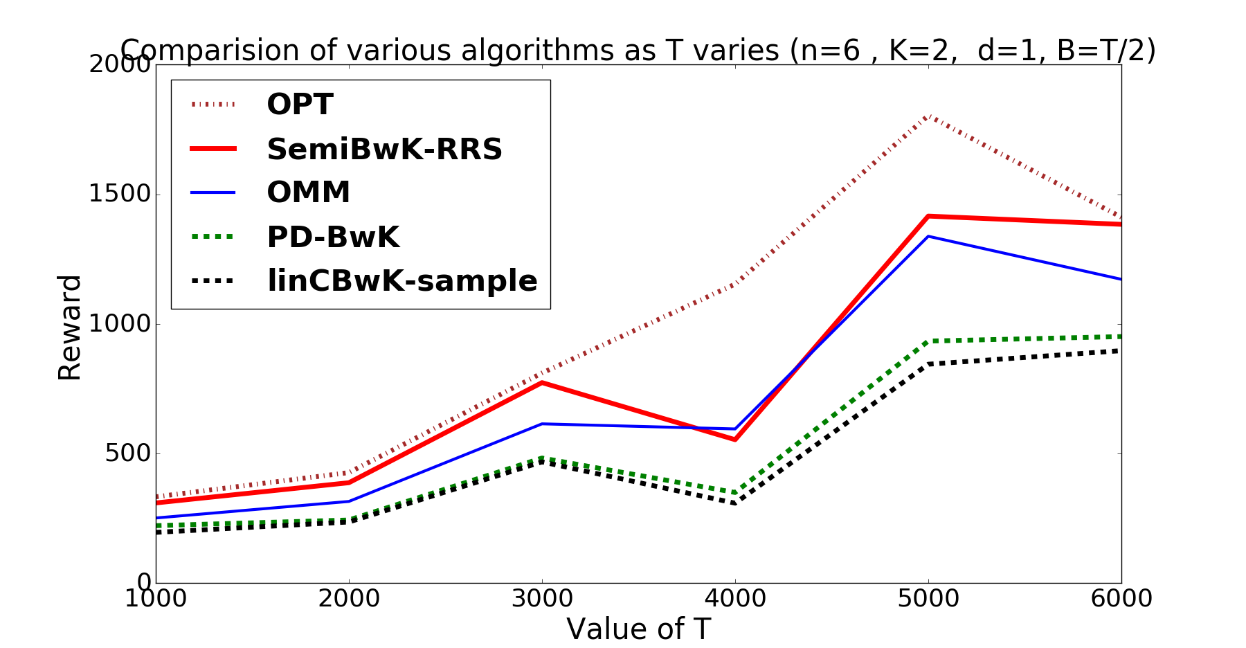
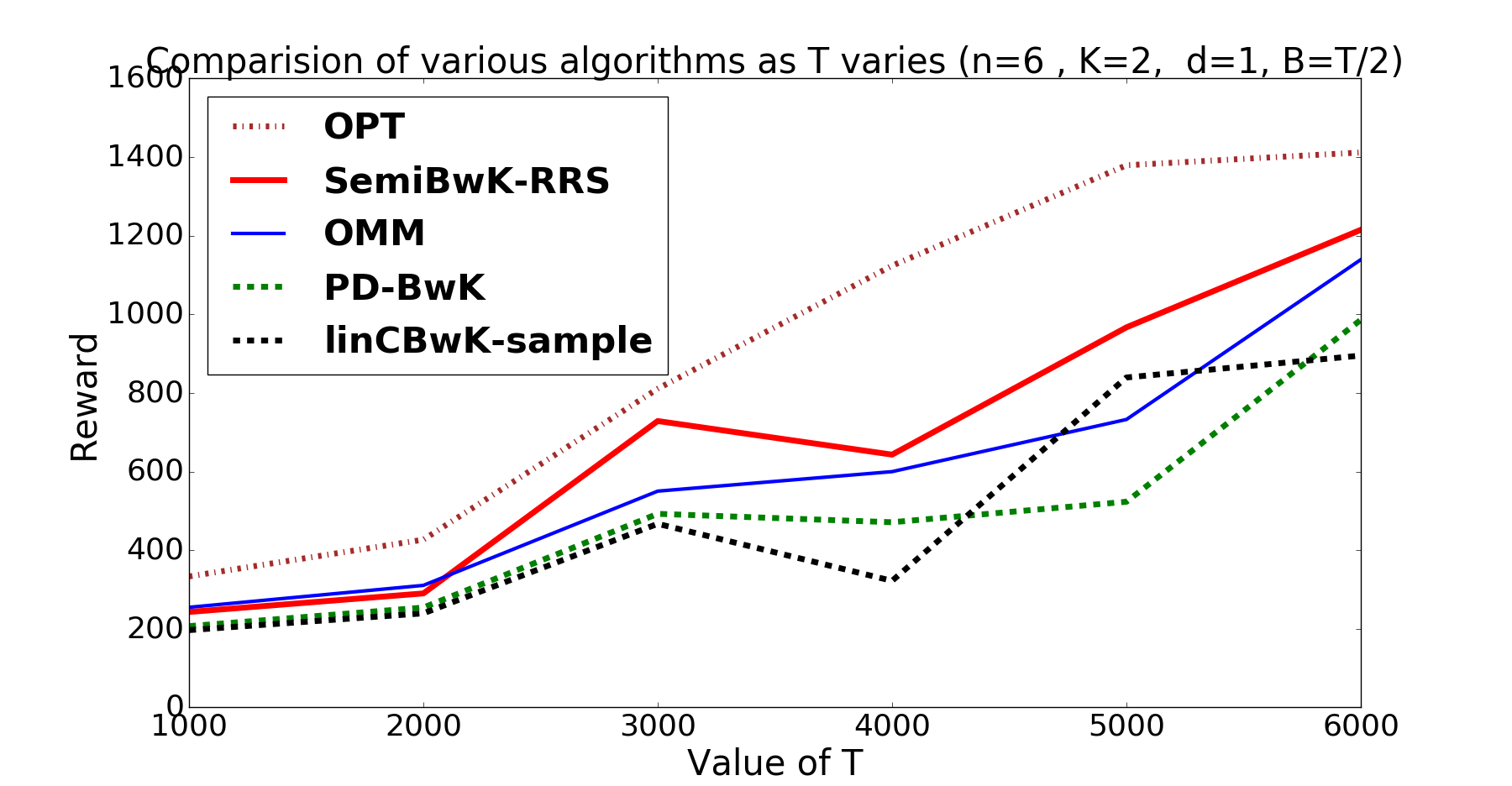
We ran some experiments on simulated datasets in order to compare our algorithm, , with some prior work that can be used to solve :
-
•
the primal-dual algorithm for from Badanidiyuru et al. (2013a), denoted .
-
•
an algorithm for combinatorial semi-bandits with a matroid constraint: “Optimistic Matroid Maximization” from Kveton et al. (2014), denoted .
-
•
the linear-contextual algorithm from Agrawal and Devanur (2016), discussed in the Introduction, denoted .
To speed up the computation in , we used a heuristic modification suggested by the authors in a private communication. This modification did not substantially affect average rewards in our preliminary experiments. We also made a heuristic improvement to our algorithm, setting and . We use the same value of for the algorithm as well.
Problem instances. We did not attempt to comprehensively cover the huge variety of problem instances in . Instead, we focus on two representative applications from Section 5.
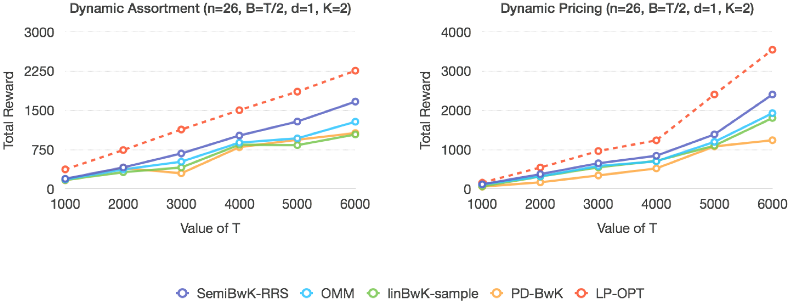
The first experiment is on dynamic assortment. We have products, and for each product there is an atom and a resource . The (fixed) price for each product is generated as an independent sample from , a uniform distribution on . At each round, we sample the buyers’s valuation from , independently for each product. If the valuation for a given product is greater than the price, one item of this product is sold (and then the reward for atom is the price, and consumption of resource is ). Else, we set reward for atom and consumption for resource to be .
The second experiment is on dynamic pricing with two products. We have allowed prices, uniformly spaced in the interval. Recall that atoms correspond to price-product pairs, for the total of atoms. In each round , the valuation for each product is chosen independently from a normal distribution truncated on . The mean valuation is drawn (once for all rounds) from . If is greater than the offered price , one item of this product is sold. Then reward for the corresponding atom is the price , and consumption of product is . If there is no sale for this product, the reward and consumption for each atom is set to .
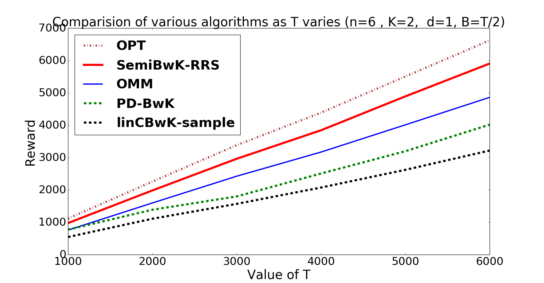
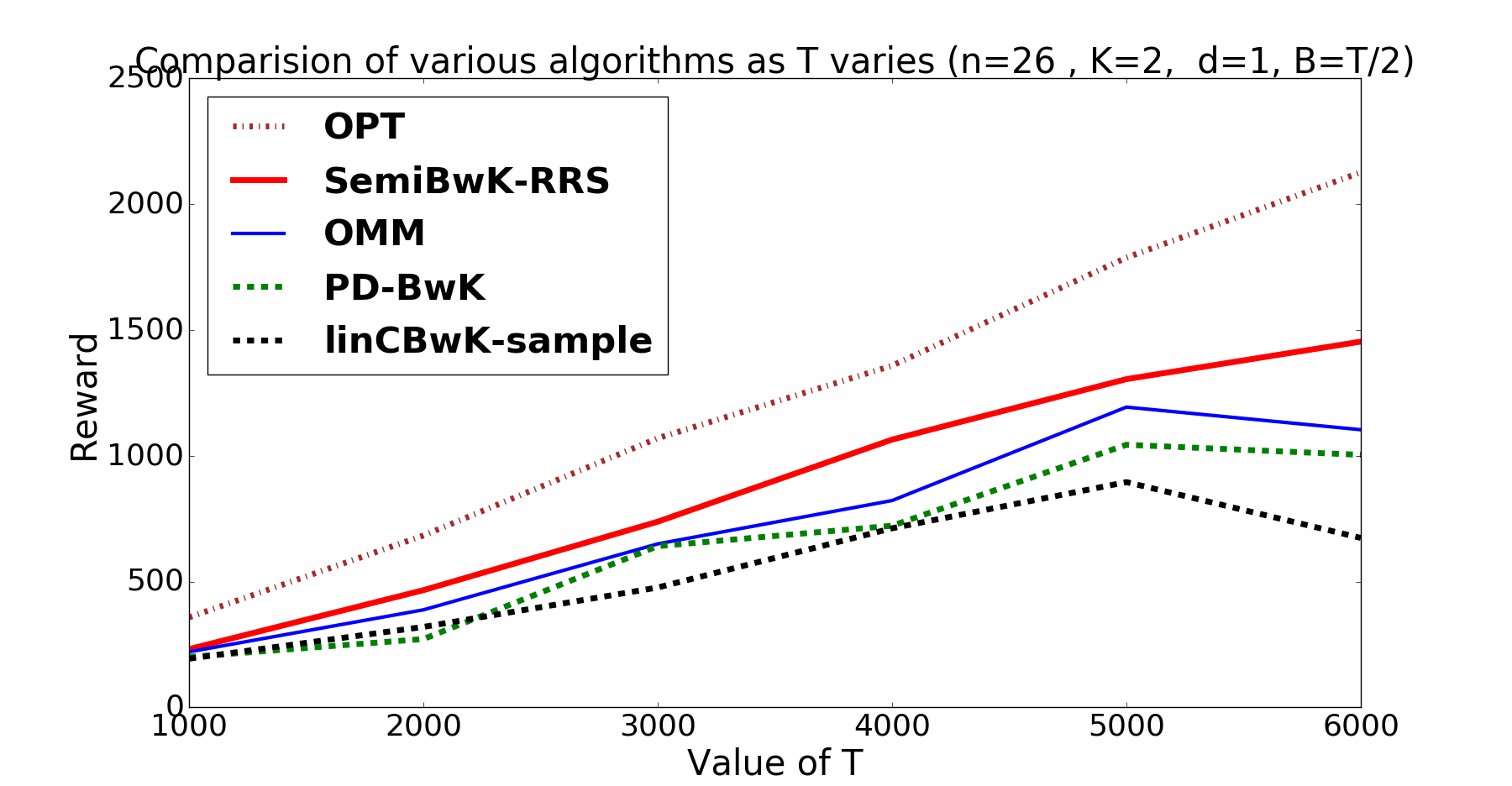
The third experiment is a modification of the dynamic assortment example, in which we ensure that even “non-action” (e.g., no sale) exhausts resources other than time. As in dynamic assortment, we have products, and for each product there is an atom and a resource . The (fixed) price for each product is generated as an independent sample from , a uniform distribution on . At each round, we sample the buyers’s valuation from , independently for each product. If the valuation for a given product is greater than the price, one item of this product is sold (and then the reward for atom is the price, and consumption of resource is ). Else, we do something different from dynamic assortment: we set reward for atom and consumption for resource to be the buyer’s valuation.
The fourth experiment is a similar modification of the dynamic pricing example. We have allowed prices, uniformly spaced in the interval. Recall that atoms correspond to price-product pairs, for the total of atoms. In each round , the valuation for each product is chosen independently from a normal distribution truncated on . The mean valuation is drawn (once for all rounds) from . If the valuation for a given product is greater than the offered price , one item of this product is sold (and then reward for the corresponding atom is the price, and consumption of product is ). If there is no sale for this product, we do something different from dynamic pricing. For each atom , if then the reward for atom is drawn independently from and resource consumption is ; else, reward is and consumption is . While dynamic assortment is modeled with a uniform matroid, and dynamic pricing is modeled with a partition matroid, we tried both matroids on each family.
Experimental setup and results. We choose various values of , and and run our algorithms on the above two datasets assuming both a uniform matroid constraint and a partition matroid constraint. We choose , and . The maximum number of atoms in any action is set to . For a given algorithm, dataset and configuration of and , we simulate each algorithm for independent runs and take the average. We calculate the total reward obtained by the algorithm at the end of time-steps.
Figure 1 shows results for the first two experiments. Figures 2 and 3 show the results on the third and fourth experiments. Our algorithm achieves the best regret among the competitors. As a benchmark, we included the performance of the fractional allocation in , denoted .

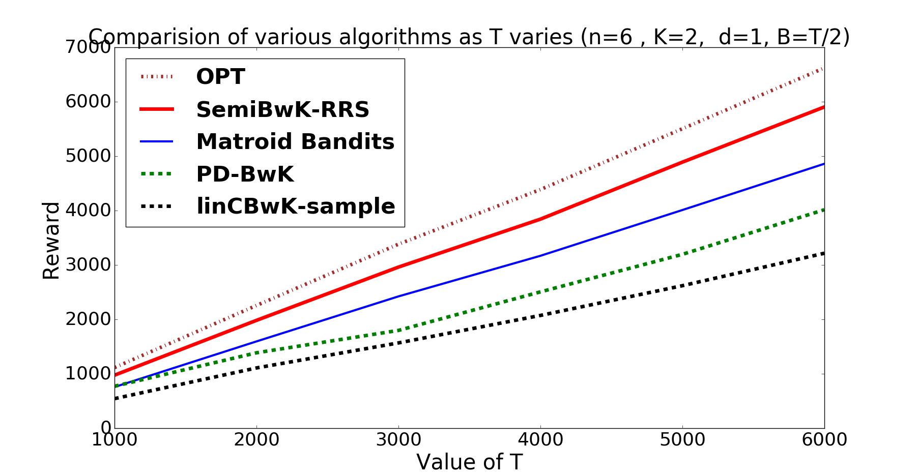
Additional experiment. and have running times proportional to the number of actions. We ran an additional experiment which compared per-step running times. We first calculate the average running time for every steps and take the median of such runs. For both Uniform matroid and Partition matroid, we run the faster RRS due to Gandhi et al. (2006). See Figure 4 for results.
Details of heuristic implementation of . We now briefly describe the heuristic we use to simulate the algorithm. Note that even though the per-time-step running time of is reasonable, it takes a significant time when we want to perform simulations for many time-steps. The time-consuming step in the algorithm is the solution to a convex program for computing the optimistic estimates (namely and ). Hence, the heuristic gives a faster way to obtain this estimate. We sample multiple times from a multi-variate Gaussian with mean and covariance (to obtain estimate ) and with mean and covariance (to obtain estimate for each resource ). We use these samples to compute the objective to choose the action at time-step . For each sample, we compute the best action based on the objective in . We finally choose the action that occurs majority number of times in these samples. The number of samples we choose is set to 30.
Language Details of algorithms. All algorithms except were implemented in Python. The algorithm was implemented in MATLAB. This difference is crucial when we compare running times since language construct can speed-up or slow down algorithms in practice. However, it is known that 101010https://www.mathworks.com/products/matlab/matlab-vs-python.html for matrix operations commonly encountered in engineering and statistics, MATLAB implementations runs several orders of magnitude faster than the corresponding python implementation. Since is the slowest of the four algorithms, our comparison of running times across languages is justified.
Acknowledgements. Karthik would like to thank Aravind Srinivasan for some useful discussions.
References
- Agarwal et al. [2016] A. Agarwal, S. Bird, M. Cozowicz, M. Dudik, J. Langford, L. Li, L. Hoang, D. Melamed, S. Sen, R. Schapire, and A. Slivkins. Multiworld testing: A system for experimentation, learning, and decision-making, 2016. A white paper, available at https://github.com/Microsoft/mwt-ds/raw/master/images/MWT-WhitePaper.pdf.
- Agrawal and Devanur [2014a] S. Agrawal and N. R. Devanur. Bandits with concave rewards and convex knapsacks. In 15th ACM Conf. on Economics and Computation (ACM EC), 2014a.
- Agrawal and Devanur [2014b] S. Agrawal and N. R. Devanur. Bandits with concave rewards and convex knapsacks. In Proceedings of the fifteenth ACM conference on Economics and computation, pages 989–1006. ACM, 2014b.
- Agrawal and Devanur [2016] S. Agrawal and N. R. Devanur. Linear contextual bandits with knapsacks. In 29th Advances in Neural Information Processing Systems (NIPS), 2016.
- Agrawal et al. [2016] S. Agrawal, N. R. Devanur, and L. Li. An efficient algorithm for contextual bandits with knapsacks, and an extension to concave objectives. In 29th Conf. on Learning Theory (COLT), 2016.
- Anantharam et al. [1987] V. Anantharam, P. Varaiya, and J. Walrand. Asymptotically efficient allocation rules for the multiarmed bandit problem with multiple plays-part i: Iid rewards. IEEE Transactions on Automatic Control, 32(11):968–976, 1987.
- Asadpour et al. [2010] A. Asadpour, M. X. Goemans, A. Madry, S. O. Gharan, and A. Saberi. An o (log n/log log n)-approximation algorithm for the asymmetric traveling salesman problem. In SODA, volume 10, pages 379–389. SIAM, 2010.
- Auer et al. [2002] P. Auer, N. Cesa-Bianchi, and P. Fischer. Finite-time analysis of the multiarmed bandit problem. Machine Learning, 47(2-3):235–256, 2002.
- Babaioff et al. [2015] M. Babaioff, S. Dughmi, R. D. Kleinberg, and A. Slivkins. Dynamic pricing with limited supply. ACM Trans. on Economics and Computation, 3(1):4, 2015. Special issue for 13th ACM EC, 2012.
- Badanidiyuru et al. [2012] A. Badanidiyuru, R. Kleinberg, and Y. Singer. Learning on a budget: posted price mechanisms for online procurement. In 13th ACM Conf. on Electronic Commerce (EC), pages 128–145, 2012.
- Badanidiyuru et al. [2013a] A. Badanidiyuru, R. Kleinberg, and A. Slivkins. Bandits with knapsacks. In 54th IEEE Symp. on Foundations of Computer Science (FOCS), 2013a.
- Badanidiyuru et al. [2013b] A. Badanidiyuru, R. Kleinberg, and A. Slivkins. Bandits with knapsacks. A technical report on arxiv.org., May 2013b.
- Badanidiyuru et al. [2014] A. Badanidiyuru, J. Langford, and A. Slivkins. Resourceful contextual bandits. In 27th Conf. on Learning Theory (COLT), 2014.
- Besbes and Zeevi [2009] O. Besbes and A. Zeevi. Dynamic pricing without knowing the demand function: Risk bounds and near-optimal algorithms. Operations Research, 57:1407–1420, 2009.
- Besbes and Zeevi [2012] O. Besbes and A. J. Zeevi. Blind network revenue management. Operations Research, 60(6):1537–1550, 2012.
- Bubeck and Cesa-Bianchi [2012] S. Bubeck and N. Cesa-Bianchi. Regret Analysis of Stochastic and Nonstochastic Multi-armed Bandit Problems. Foundations and Trends in Machine Learning, 5(1), 2012.
- Cesa-Bianchi et al. [2013] N. Cesa-Bianchi, C. Gentile, and Y. Mansour. Regret minimization for reserve prices in second-price auctions. In ACM-SIAM Symp. on Discrete Algorithms (SODA), 2013.
- Chekuri et al. [2010] C. Chekuri, J. Vondrak, and R. Zenklusen. Dependent randomized rounding via exchange properties of combinatorial structures. In Foundations of Computer Science (FOCS), 2010 51st Annual IEEE Symposium on, pages 575–584. IEEE, 2010.
- Chekuri et al. [2011] C. Chekuri, J. Vondrák, and R. Zenklusen. Multi-budgeted matchings and matroid intersection via dependent rounding. In Proceedings of the twenty-second annual ACM-SIAM symposium on Discrete Algorithms, pages 1080–1097. SIAM, 2011.
- Chen et al. [2013] W. Chen, Y. Wang, and Y. Yuan. Combinatorial multi-armed bandit: General framework and applications. In S. Dasgupta and D. Mcallester, editors, Proceedings of the 30th International Conference on Machine Learning (ICML-13), volume 28, pages 151–159. JMLR Workshop and Conference Proceedings, 2013.
- Combes et al. [2015a] R. Combes, C. Jiang, and R. Srikant. Bandits with budgets: Regret lower bounds and optimal algorithms. ACM SIGMETRICS Performance Evaluation Review, 43(1):245–257, 2015a.
- Combes et al. [2015b] R. Combes, M. S. T. M. Shahi, A. Proutiere, et al. Combinatorial bandits revisited. In Advances in Neural Information Processing Systems, pages 2116–2124, 2015b.
- Gai et al. [2010] Y. Gai, B. Krishnamachari, and R. Jain. Learning multiuser channel allocations in cognitive radio networks: A combinatorial multi-armed bandit formulation. In New Frontiers in Dynamic Spectrum, 2010 IEEE Symposium on, pages 1–9. IEEE, 2010.
- Gai et al. [2012] Y. Gai, B. Krishnamachari, and R. Jain. Combinatorial network optimization with unknown variables: Multi-armed bandits with linear rewards and individual observations, Oct. 2012.
- Gandhi et al. [2006] R. Gandhi, S. Khuller, S. Parthasarathy, and A. Srinivasan. Dependent rounding and its applications to approximation algorithms. Journal of the ACM (JACM), 53(3):324–360, 2006.
- Gittins et al. [2011] J. Gittins, K. Glazebrook, and R. Weber. Multi-Armed Bandit Allocation Indices. John Wiley & Sons, 2011.
- Guha and Munagala [2007] S. Guha and K. Munagala. Multi-armed Bandits with Metric Switching Costs. In 36th Intl. Colloquium on Automata, Languages and Programming (ICALP), pages 496–507, 2007.
- Gupta et al. [2011] A. Gupta, R. Krishnaswamy, M. Molinaro, and R. Ravi. Approximation algorithms for correlated knapsacks and non-martingale bandits. In 52nd IEEE Symp. on Foundations of Computer Science (FOCS), pages 827–836, 2011.
- György et al. [2007] A. György, T. Linder, G. Lugosi, and G. Ottucsák. The on-line shortest path problem under partial monitoring. J. of Machine Learning Research (JMLR), 8:2369–2403, 2007.
- Impagliazzo and Kabanets [2010] R. Impagliazzo and V. Kabanets. Constructive proofs of concentration bounds. In Approximation, Randomization, and Combinatorial Optimization. Algorithms and Techniques, pages 617–631. Springer, 2010.
- Katariya et al. [2016] S. Katariya, B. Kveton, C. Szepesvári, and Z. Wen. DCM bandits: Learning to rank with multiple clicks. In Proceedings of the 33nd International Conference on Machine Learning, ICML 2016, New York City, NY, USA, June 19-24, 2016, pages 1215–1224, 2016.
- Kleinberg et al. [2015] R. Kleinberg, A. Slivkins, and E. Upfal. Bandits and experts in metric spaces. Working paper, published at http://arxiv.org/abs/1312.1277, 2015. Merged and revised version of conference papers in ACM STOC 2008 and ACM-SIAM SODA 2010.
- Krishnamurthy et al. [2016] A. Krishnamurthy, A. Agarwal, and M. Dudík. Contextual semibandits via supervised learning oracles. In 29th Advances in Neural Information Processing Systems (NIPS), 2016.
- Kveton et al. [2014] B. Kveton, Z. Wen, A. Ashkan, H. Eydgahi, and B. Eriksson. Matroid bandits: Fast combinatorial optimization with learning. In N. L. Zhang and J. Tian, editors, UAI, pages 420–429. AUAI Press, 2014.
- Kveton et al. [2015a] B. Kveton, C. Szepesvari, Z. Wen, and A. Ashkan. Cascading bandits: Learning to rank in the cascade model. In D. Blei and F. Bach, editors, Proceedings of the 32nd International Conference on Machine Learning (ICML-15), pages 767–776. JMLR Workshop and Conference Proceedings, 2015a.
- Kveton et al. [2015b] B. Kveton, Z. Wen, A. Ashkan, and C. Szepesvári. Tight regret bounds for stochastic combinatorial semi-bandits. In G. Lebanon and S. V. N. Vishwanathan, editors, AISTATS, JMLR Workshop and Conference Proceedings. JMLR.org, 2015b.
- Lai and Robbins [1985] T. L. Lai and H. Robbins. Asymptotically efficient Adaptive Allocation Rules. Advances in Applied Mathematics, 6:4–22, 1985.
- Papadimitriou and Steiglitz [1982] C. H. Papadimitriou and K. Steiglitz. Combinatorial optimization: algorithms and complexity. Courier Corporation, 1982.
- Raghavan and Tompson [1987] P. Raghavan and C. D. Tompson. Randomized rounding: a technique for provably good algorithms and algorithmic proofs. Combinatorica, 7(4):365–374, 1987.
- Rakhlin and Sridharan [2016] A. Rakhlin and K. Sridharan. BISTRO: an efficient relaxation-based method for contextual bandits. In 33nd Intl. Conf. on Machine Learning (ICML), 2016.
- Robbins [1952] H. Robbins. Some Aspects of the Sequential Design of Experiments. Bull. Amer. Math. Soc., 58:527–535, 1952.
- Schrijver [2002] A. Schrijver. Combinatorial optimization: polyhedra and efficiency, volume 24. Springer Science & Business Media, 2002.
- Singla and Krause [2013] A. Singla and A. Krause. Truthful incentives in crowdsourcing tasks using regret minimization mechanisms. In 22nd Intl. World Wide Web Conf. (WWW), pages 1167–1178, 2013.
- Slivkins [2013] A. Slivkins. Dynamic ad allocation: Bandits with budgets. A technical report on arxiv.org/abs/1306.0155, June 2013.
- Slivkins and Vaughan [2013] A. Slivkins and J. W. Vaughan. Online decision making in crowdsourcing markets: Theoretical challenges. SIGecom Exchanges, 12(2), December 2013.
- Syrgkanis et al. [2016] V. Syrgkanis, A. Krishnamurthy, and R. E. Schapire. Efficient algorithms for adversarial contextual learning. In 33nd Intl. Conf. on Machine Learning (ICML), 2016.
- Thompson [1933] W. R. Thompson. On the likelihood that one unknown probability exceeds another in view of the evidence of two samples. Biometrika, 25(3-4):285 294, 1933.
- Tran-Thanh et al. [2010] L. Tran-Thanh, A. Chapman, E. M. de Cote, A. Rogers, and N. R. Jennings. -first policies for budget-limited multi-armed bandits. In 24th AAAI Conference on Artificial Intelligence (AAAI), pages 1211–1216, 2010.
- Tran-Thanh et al. [2012] L. Tran-Thanh, A. Chapman, A. Rogers, and N. R. Jennings. Knapsack based optimal policies for budget-limited multi-armed bandits. In 26th AAAI Conference on Artificial Intelligence (AAAI), pages 1134–1140, 2012.
- Wang et al. [2014] Z. Wang, S. Deng, and Y. Ye. Close the gaps: A learning-while-doing algorithm for single-product revenue management problems. Operations Research, 62(2):318–331, 2014.
- Wen et al. [2015] Z. Wen, B. Kveton, and A. Ashkan. Efficient learning in large-scale combinatorial semi-bandits. In F. R. Bach and D. M. Blei, editors, ICML, JMLR Workshop and Conference Proceedings, pages 1113–1122. JMLR.org, 2015.
- Williamson and Shmoys [2011] D. P. Williamson and D. B. Shmoys. The design of approximation algorithms. Cambridge university press, 2011.
- Xia et al. [2016a] Y. Xia, W. Ding, X.-D. Zhang, N. Yu, and T. Qin. Budgeted bandit problems with continuous random costs. In Asian Conference on Machine Learning, pages 317–332, 2016a.
- Xia et al. [2016b] Y. Xia, T. Qin, W. Ma, N. Yu, and T.-Y. Liu. Budgeted multi-armed bandits with multiple plays. In Proceedings of the Twenty-Fifth International Joint Conference on Artificial Intelligence, IJCAI’16, pages 2210–2216. AAAI Press, 2016b. ISBN 978-1-57735-770-4. URL http://dl.acm.org/citation.cfm?id=3060832.3060930.
- Zong et al. [2016] S. Zong, H. Ni, K. Sung, N. R. Ke, Z. Wen, and B. Kveton. Cascading bandits for large-scale recommendation problems. 2016.
Appendix A Proof of Theorem in Preliminaries
Appendix B Matroid constraints
To make this paper more self-contained, we provide more background on matroid constraints and special cases thereof.
Recall that in , we have a finite ground set whose elements are called “atoms”, and a family of “feasible subsets” of the ground set which are the actions. To be consistent with the literature on matroids, the ground set will be denoted . Family of subsets of is called a matroid if it satisfies the following properties:
-
•
Empty set: The empty set is present in
-
•
Hereditary property: For two subsets such that , we have that
-
•
Exchange property: For and , we have that
Matroids are linearizable, i.e., the convex hull of forms a polytope in . (Here subsets of are intepreted as binary vectors in .) In other words, there exists a set of linear constraints whose set of feasible integral solutions is . In fact, the convex hull of , a.k.a. the matroid polytope, can be represented via the following linear system:
| (LP-Matroid) |
Here , and is the “rank function” for .
is indeed the set of all feasible integral solutions of the above system. This is a standard fact in combinatorial optimization, e.g., see Theorem 40.2 and its corollaries in Schrijver [2002].
We will now describe some well-studied special cases of matroids. That they indeed are special cases of matroids is well-known, we will not present the corresponding proofs here.
In all LPs presented below, we have variables for each arom , and we use shorthand for .
Cardinality constraints. Cardinality constraint is defined as follows: a subset of atoms belongs to if and only if for some fixed . This is perhaps the simplest constraint that our results are applicable to. In the context of , each action selects at most atoms.
The corresponding induced polytope is as follows:
| (LP-Cardinality) |
Partition matroid constraints. A generalization of cardinality constraints, called partition matroid constraints, is defined as follows. Suppose we have a collection of disjoint subsets of , and numbers . A subset of atoms belongs to if and only if for every . Partition matroid constraints appear in several applications of such as dynamic pricing, adjusting repeated auctions, and repeated bidding. In these applications, each action selects one price/bid for each offered product. Also, partition matroid constraints can model clusters of mutually exclusive products in dynamic assortment application.
The induced polytope is as follows:
| (LP-PartitionMatroid) |
Spanning tree constraints. Spanning tree constraints describe spanning trees in a given undirected graph , where the atoms correspond to edges in the graph. A spanning tree in is a subset of edges such that is a tree. Action set consists of all spanning trees of .
The induced polytope is as follows:
| (LP-SpanningTree) |
Here, denotes the edge set in subgraph induced by node set .