\pkgFRK: An \proglangR Package for Spatial and Spatio-Temporal Prediction with Large Datasets
Andrew Zammit-Mangion, Noel Cressie \PlaintitleFRK: An R package for spatial and spatio-temporal prediction with large datasets \Shorttitle\pkgFRK: An \proglangR package for spatial and spatio-temporal prediction with large datasets \Abstract
\pkgFRK is an \proglangR software package for spatial/spatio-temporal modelling and prediction with large datasets. It facilitates optimal spatial prediction (kriging) on the most commonly used manifolds (in Euclidean space and on the surface of the sphere), for both spatial and spatio-temporal fields. It differs from many of the packages for spatial modelling and prediction by avoiding stationary and isotropic covariance and variogram models, instead constructing a spatial random effects (SRE) model on a fine-resolution discretised spatial domain. The discrete element is known as a basic areal unit (BAU), whose introduction in the software leads to several practical advantages. The software can be used to (i) integrate multiple observations with different supports with relative ease; (ii) obtain exact predictions at millions of prediction locations (without conditional simulation); and (iii) distinguish between measurement error and fine-scale variation at the resolution of the BAU, thereby allowing for reliable uncertainty quantification. The temporal component is included by adding another dimension. A key component of the SRE model is the specification of spatial or spatio-temporal basis functions; in the package, they can be generated automatically or by the user. The package also offers automatic BAU construction, an expectation-maximisation (EM) algorithm for parameter estimation, and functionality for prediction over any user-specified polygons or BAUs. Use of the package is illustrated on several spatial and spatio-temporal datasets, and its predictions and the model it implements are extensively compared to others commonly used for spatial prediction and modelling.
\Keywordsbasic areal units, EM algorithm, fixed rank kriging, spatial random effects model, spatial prediction
\PlainkeywordsFixed rank kriging, basic areal units, EM algorithm, spatial prediction, spatial random effects model \Address
Andrew Zammit-Mangion
National Institute for Applied Statistics Research Australia (NIASRA)
School of Mathematics and Applied Statistics
University of Wollongong
Wollongong, Australia
E-mail:
URL: https://andrewzm.wordpress.com
1 Introduction
Fixed rank kriging (FRK) is a spatial/spatio-temporal modelling and prediction framework that is scaleable, works well with large datasets, and can deal easily with data that have different spatial supports. FRK hinges on the use of a spatial random effects (SRE) model, in which a spatially correlated mean-zero random process is decomposed using a linear combination of spatial basis functions with random coefficients plus a term that captures the random process’ fine-scale variation. Dimensionality reduction through a relatively small number of basis functions ensures computationally efficient prediction, while the reconstructed spatial process is, in general, non-stationary. The SRE model has a spatial covariance function that is always nonnegative-definite and, because any (possibly non-orthogonal) basis functions can be used, it can be constructed so as to approximate standard families of covariance functions (Kang_2011). For a detailed treatment of FRK, see Cressie_2006; Cressie_2008, Shi_2007, and Nguyen_2012.
There are numerous \proglangR (R) packages available for modelling and prediction with spatial or spatio-temporal data,111see https://cran.r-project.org/web/views/Spatial.html. although relatively few of these make use of a model with spatial basis functions. A few variants of FRK have been developed to date, and the one that comes closest to the present software is \pkgLatticeKrig (Nychka_2015; LatticeKrig). \pkgLatticeKrig implements what we call a LatticeKrig model, which is made up of Wendland basis functions (that have compact support) decomposing a spatially correlated process. LatticeKrig models use a Markov assumption to construct a precision matrix (the matrix in Section 2.1) to describe the dependence between the coefficients of these basis functions. This, in turn, results in efficient computations and the potential use of a large number () of basis functions. LatticeKrig models do not cater for what we term fine-scale-process variation and, instead, the finest scale of the process is limited to the finest resolution of the basis functions used.
The package \pkgINLA (Lindgren_2015) is a general-purpose package for model fitting and prediction. One advantage of \pkgINLA is that it contains functionality for fitting Gaussian processes that have covariance functions from the Matérn class (see Lindgren_2015, for details on software interface) by approximating a stochastic partial differential equation (SPDE) using a Gaussian Markov random field (GMRF). Specifically, the process is decomposed using basis functions that are triangular ‘tent’ functions, and the coefficients of these basis functions are normally distributed with a sparse precision matrix. Thus, these models, which we term SPDE–GMRF models, share many of the features of LatticeKrig models. A key advantage of \pkgINLA over \pkgLatticeKrig is that once the spatial or spatio-temporal model is constructed, one has access to all the approximate-inference machinery and likelihood models available within the package.
Kang_2011 develop Bayesian FRK; they keep the spatial basis functions fixed and put a prior distribution on K. The predictive-process approach of Banerjee_2008 can also be seen as a type of Bayesian FRK, where the basis functions are constructed from the postulated covariance function of the spatial random effects and hence depend on parameters (see Katzfuss_2014, for an equivalence argument). An \proglangR package that implements predictive processes is \pkgspBayes (Finley_2007). It allows for multivariate spatial or spatio-temporal processes, and Bayesian inference is carried out using Markov chain Monte Carlo (MCMC), thus allowing for a variety of likelihood models. Because the implied basis functions are constructed based on a parametric covariance model, a prior distribution on parameters results in new basis functions generated at each MCMC iteration. Since this can slow down the computation, the number of knots used in predictive processes is usually chosen to be small, which has the effect of limiting their ability to model finer scales.
Our software package \pkgFRK differs from spatial prediction packages currently available by constructing an SRE model on a discretised domain, where the discrete element is known as a basic areal unit (BAU; see, e.g., Nguyen_2012). The BAU can be viewed as the smallest spatial area or spatio-temporal volume that can be resolved by the process and, to reflect this, the process itself is assumed to be piecewise constant over the set of BAUs. The BAUs serve many purposes in FRK: They define a fine grid over which to do numerical integrations for change-of-support problems; a fine lattice of discrete points over which to predict (although \pkgFRK implements functions to predict over any arbitrary user-defined polygons); and a set of bins within which to average large spatio-temporal datasets, if so desired, for computational efficiency. BAUs do not need to be square or all equal in size, but they do need to be ‘small,’ in the sense that they should be able to reconstruct the (undiscretised) process with minimal error.
In the standard ‘flavour’ of FRK (Cressie_2008), which we term vanilla FRK (FRK-V), there is an explicit reliance on multi-resolution basis functions to give complex non-stationary spatial patterns at the cost of not imposing any structure on K, the covariance matrix of the basis function weights. This can result in identifiability issues and hence in over-fitting the data when K is estimated using standard likelihood methods (e.g., Nguyen_2014), especially in regions of data paucity. Therefore, in \pkgFRK we also implement a model (FRK-M) where a parametric structure is imposed on K (e.g., Stein_2008; Nychka_2015). The main aim of the package \pkgFRK is to facilitate spatial and spatio-temporal analysis and prediction for large datasets, where multiple observatons come with different spatial supports. We see that in ‘big data’ scenarios, lack of consideration of fine-scale variation may lead to over-confident predictions, irrespective of the number of basis functions adopted.
In Section 2, we describe the modelling, estimation, and prediction approach we adopt in \pkgFRK. In Section 3, we discuss further details of the package and provide a simple example on the classic \codemeuse dataset. In Section 4, we evaluate the SRE model implemented in \pkgFRK in controlled cases, against LatticeKrig models and SPDE–GMRF models through use of the packages \pkgLatticeKrig and \pkgINLA. In Section 5, we show its capability to deal with change-of-support issues and anisotropic processes. In Section 6, we show how to use \pkgFRK with spatio-temporal data and illustrate its use on the modelling and prediction of column-averaged carbon dioxide on the globe from remote sensing data produced by NASA’s OCO-2 mission. The spatio-temporal dataset contains millions of observations. Finally, Section 7 discusses future work.
2 Outline of \pkgFRK: Modelling, estimation and prediction
In this section we present the theory behind the operations implemented in \pkgFRK. In Section 2.1 we introduce the SRE model, in Section 2.2 we discuss the EM algorithm for parameter estimation, and in Section 2.3 we present the spatial prediction equations.
2.1 The SRE model
Denote the spatial process of interest as , where s indexes the location of in our domain of interest . In what follows, we assume that is a spatial domain but extensions to spatio-temporal domains are natural within the framework (Section LABEL:sec:ST). Consider the classical spatial statistical model,
where, for , is a vector of spatially referenced covariates, is a vector of regression coefficients, is a small-scale, spatially correlated random effect, and is a fine-scale random effect that is ‘almost’ spatially uncorrelated. It is natural to let . Define , so that . It is the structure of the process in terms of a linear combination of a fixed number of spatial basis functions that defines the SRE model for :
where is an -variate random vector, and is an -dimensional vector of pre-specified spatial basis functions. Sometimes, contains basis functions of multiple resolutions (e.g., wavelets), they may or may not be orthogonal, and they may or may not have compact support. The basis functions chosen should be able to adequately reconstruct realisations of ; an empirical spectral-based approach that can ensure this is discussed in Zammit_2012.
In order to cater for different observation supports (defined below), it is convenient to assume a discretised domain of interest that is made up of small, non-overlapping basic areal units or BAUs (Nguyen_2012), and . The set of BAUs is a discretisation, or ‘tiling,’ of the original domain , and typically . The process is then averaged over the BAUs, giving the vector , where
| (1) |
and is the number of BAUs. At this BAU level,
| (2) |
where for , , and is specified below. The SRE model specifies that the small-scale random variation is and hence in terms of the discretisation onto ,
so that , where S is the matrix defined as follows:
| (3) |
In \pkgFRK, we assume that is an -dimensional Gaussian vector with mean zero and covariance matrix K, and estimation of K is based on likelihood methods; we denote this variant of FRK as FRK-V (where recall that ‘V’ stands for ‘vanilla’). If some structure is imposed on in terms of parameters , then and needs to be estimated; we denote this variant as FRK-M (where recall that ‘M’ stands for ‘model’). Frequently, the resolution of the BAUs is sufficiently fine, and the basis functions are sufficiently smooth, so that S can be approximated:
| (4) |
where are the centroids of the BAUs. Since small BAUs are always assumed, this approximation is used throughout \pkgFRK.
In \pkgFRK, we do not directly model , since we are only interested in its discretised version. Rather, we assume that has a Gaussian distribution with mean zero and variance
where is a parameter to be estimated, and the weights are known and represent heteroscedasticity. These weights are typically generated from domain knowledge; they may, for example, correspond to topographical features such as terrain roughness (Zammit_2015). Since we specified to be ‘almost’ spatially uncorrelated, it is reasonable to assume that the variables representing the discretised fine-scale variation, , are uncorrelated. From (2), we can write
| (5) |
where , , and , for known .
We now assume that the hidden (or latent) process, , is observed with footprints (possibly overlapping) spanning one or more BAUs, where typically (note that both and are possible). We thus define the observation domain as , where is a non-empty set in , the power set of , and . For illustration, consider the simple case of the discretised domain being made up of three BAUs. Then and, for example, , where (i.e., ) and (i.e., ). Catering for different footprints is important for remote sensing applications in which satellite-instrument footprints can widely differ (e.g., Zammit_2015).
Each is either a BAU or a union of BAUs. Measurement of is imperfect: We define the measurement process as noisy measurements of the process averaged over the footprints
| (6) |
where the weights,
depend on the areas of the BAUs, and is the indicator function. Currently, in \pkgFRK, BAUs of equal area are assumed, but we give (6) in its most general form. The random quantities and capture the imperfections of the measurement. Better known is the measurement-error component , which is assumed to be mean-zero Gaussian distributed. The component captures any bias in the measurement at the BAU level, which has the interpretation of an intra-BAU systematic error. These systematic errors are BAU-specific, that is, the are uncorrelated with mean zero and variance
where is a parameter to be estimated, and represent known heteroscedasticity.
We assume that and are independent. We also assume that the observations are conditionally independent, when conditioned on and . Equivalently, we assume that the measurement errors are independent with .
We represent the data as . Then, since each element in is the union of subsets of , one can construct a matrix
such that
where the three components are independent, , and is an diagonal covariance matrix. The matrix is assumed known from the properties of the measurement. If it is not known, is fixed to I and is estimated using variogram techniques (Kang_2009). Notice that the rows of the matrix sum to 1.
It will be convenient to re-write
| (7) |
where , , , , , , and where is known. Then, recalling that and ,
In practice, it is not always possible for each to include entire BAUs. For simplicity, in \pkgFRK we assume that the observation footprint overlaps a BAU if and only if the BAU centroid lies within the footprint. Frequently, point-referenced data is included in . In this case, each data point is attributed to a specific BAU and it is possible to have multiple observations of the process defined on the same BAU.
We collect the unknown parameters in the set for FRK-V and for FRK-M for which ; their estimation is the subject of Section 2.2. If the parameters in or are known, an inversion that uses the Sherman–Woodbury identity (Henderson_1981) allows spatial prediction at any BAU in . Estimates of are substituted into these spatial predictors to yield FRK-V. Similarly, estimates of substituted into the spatial-prediction equations yield FRK-M.
In \pkgFRK, we allow the prediction set to be as flexible as ; specifically, , where is a non-empty set in and is the number of prediction areas. We can thus predict both at the individual BAU level or averages over an area spanning multiple BAUs, and these prediction regions may overlap. This is an important change-of-support feature of \pkgFRK. We provide the FRK equations in Section 2.3.
2.2 Parameter estimation using an EM algorithm
In all its generality, parameter estimation with the model of Section 2.1 is problematic due to confounding between and . In \pkgFRK, the user thus needs to choose between modelling the intra-BAU systematic errors (in which case is fixed to 0) or the process’ fine-scale variation (in which case is fixed to 0). We describe below the estimation procedure for the latter case; due to symmetry, the estimation equations of the former case can be simply obtained by replacing the subscript with . However, which case is chosen by the user has a considerable impact on the prediction equations for (Section 2.3). Recall that the measurement-error covariance matrix is assumed known from measurement characteristics, or estimated using variogram techniques prior to estimating the remaining parameters described below. For conciseness, in this section we use to denote the parameters in both FRK-V and FRK-M, only distinguishing when necessary.
We carry out parameter estimation using an expectation maximisation (EM) algorithm (similar to Katzfuss_2011; Nguyen_2014) with (7) as our model. Define the complete-data likelihood (with integrated out), where denotes the probability distribution of its argument. The EM algorithm proceeds by first computing the conditional expectation (conditional on the data) of the complete-data log-likelihood at the current parameter estimates (the E-step) and, second, maximising this function with respect to the parameters (the M-step). In mathematical notation, in the E-step the function
is found for some current estimate . In the M-step, the updated parameter estimates
are found.
The E-step boils down to finding the conditional distribution of at the current parameter estimates. One can use standard results in Gaussian conditioning (e.g., Rasmussen_2006, Appendix A) to show from the joint distribution, , that
where
where and where is defined below.
The update for is
| (8) |
In FRK-V, the update for is
while in FRK-M, where recall that , the update is
which is numerically optimised using the function \codeoptim with as the initial vector.
The update for requires the solution to
| (9) |
where
| (10) |
The solution to (9), namely , is found numerically using \codeuniroot after (8) is substituted into (10). Then is found by substituting into (8). Computational simplifications are possible when and are diagonal, since then only the diagonal of needs to be computed. Further simplifications are possible when and are proportional to the identity matrix, with constants of proportionality and , respectively. In this case,
where recall that is the dimension of the data vector and is, in this special case, the ordinary-least-squares estimate given (see (8)). These simplifications are used by \pkgFRK whenever possible.
Convergence of the EM algorithm is assessed using the (incomplete-data) log-likelihood function at each iteration,
where
and recall that . Efficient computation of the log-likelihood is facilitated through the use of the Sherman–Morrison–Woodbury matrix identity and a matrix-determinant lemma (e.g., Henderson_1981). Specifically, the operations
ensure that we only deal with vectors of length and matrices of size , where typically the fixed rank the dataset size.
2.3 Prediction
The prediction task is to make inference on the hidden -process over a set of prediction regions . Consider the process , which is derived from the process and, similar to the observations, is constructed using the BAUs . Here, is the number of areas at which spatial prediction takes place, and is equal to . Then,
where the weights are
Define . Then, since each element in is the union of subsets of , one can construct a matrix,
| (11) |
the rows of which sum to 1, such that
where , , and . As with the observations, the prediction regions may overlap. In practice, it may not always be possible for each to include entire BAUs. In this case, we assume that a prediction region contains a BAU if and only if the BAU centroid lies within the region.
Let denote the EM iteration number at which convergence is deemed to have been reached. The final estimates are then
Recall from Section 2.2 that the user needs to attribute fine-scale variation at the BAU level to either the measurement process or the hidden process . This leads to the following two cases.
Case 1: and estimate . The prediction vector and covariance matrix , corresponding to the first two moments from the predictive distribution when are
Under the assumptions taken, is a distribution. Note that all calculations are made after substituting in the EM-estimated parameters, and that is present in the estimated parameters.
Case 2: and estimate (Default). To cater for arbitrary observation and prediction support, we predict by first carrying out prediction over the full vector , that is, at the BAU level, and then transforming linearly to obtain through the use of the matrix . It is easy to see that if is an optimal (squared-error-loss matrix criterion) predictor of , then is an optimal predictor of , where A is any matrix with columns.
Let and . Then (5) can be re-written as , and
| (12) |
for
and the block-diagonal matrix , where returns a block diagonal matrix of its matrix arguments. Note that all calculations are made after substituting in the EM-estimated parameters.
For both Cases 1 and 2 it follows that and
| (13) |
3 \pkgFRK-package structure and usage
In this section we discuss the layout and the interface of the package, and we show its use on the \codemeuse dataset under ‘simple usage’ and ‘advanced usage.’ The former attempts to construct the SRE model automatically from characteristics of the data, while the latter gives the user more control through use of additional commands. The \codemeuse dataset is not large and contains 155 readings of heavy-metal abundance in a region of The Netherlands along the river Meuse. For more details on the dataset see the vignette titled ‘gstat’ in the package \pkggstat.
3.1 Usage overview
By leveraging the flexibility of the spatial and spatio-temporal objects in the \pkgsp (Bivand_2013) and \pkgspacetime (Pebesma_2012) packages, \pkgFRK provides a consistent, easy-to-use interface for the user, irrespective of whether the datasets have different spatial supports, irrespective of the manifold being used, irrespective of whether or not a temporal dimension needs to be included, and irrespective of the ‘prediction resolution.’
In Figure 1 we provide a partial unified modelling language (UML) diagram summarising the important package classes and their interaction with the packages \pkgsp and \pkgspacetime, while in Table 1 we provide a brief summary of these classes. BAUs should be \codeSpatial or \codeST pixel or polygon objects, while the data can also be point objects (although they are subsequently mapped to BAUs by \pkgFRK). Each \codeSpatial and \codeST object is equipped with a coordinate reference system (CRS), which needs to be identical across objects. The main class is the \codeSRE class, the object of which incorporates all information about fitting and prediction using the data, BAUs, and basis functions.
| Class | Description |
|---|---|
| \codeBasis | Defines basis functions on a specified manifold. |
| \codeBasis_obj | A virtual class that other basis classes inherit from. |
| \codemanifold | A virtual class that other manifold classes inherit from. |
| \codemeasure | Defines objects that compute distances on a specified manifold. |
| \codeplane, real_line, sphere, STplane, STsphere, STmanifold | Subclasses that inherit from the virtual class manifold. |
| \codeSRE | Defines the spatial-random-effects model, which is used to do FRK. |
| \codeTensorP_Basis | Tensor product of two basis functions. |
The basis functions are constructed on a manifold which, at the time of writing, can be (\codereal_line), (\codeplane), (surface of \codesphere), and their spatio-temporal counterparts (\codeSTplane and \codeSTsphere). Some consistency checks are made to ensure that the CRS in the BAUs and the data objects are compatible with the manifold on which the basis functions are constructed. As with \codespDists in the \pkgsp package, distances on the manifold are either Euclidean or great-circle. The function \codespDists in \pkgsp is not used, rather a function in an object of class \codemeasure is used for abstraction – this redundant structure is intended to facilitate future implementation of \pkgFRK on arbitrary manifolds and with arbitrary distance functions. The package \pkgFRK has support for spatio-temporal data (see Section LABEL:sec:ST); in this case, basis functions are of class \codeTensorP_Basis and, as the name implies, are constructed through the tensor product of spatial and temporal basis functions.
The package is built around a straightforward model (outlined in Section 2) and has the capability of handling large datasets (up to a few hundred thousand data points on a standard desktop machine, and a few million on a big memory machine). For linear algebraic calculations, it leverages routines from the \pkgsparseinv package (sparseinv_2018, which is built from C code written by Sparseinv) and the \proglangR package \pkgMatrix (Matrix_2015). The package \pkgINLA (Lindgren_2015) is used for finding a non-convex hull of the data points and for placing basis functions irregularly in the domain (if desired).
The user has two levels of control; for simple problems one can call the function \codeFRK, in which case basis-function construction and BAU generation is done automatically based on characteristics of the data. Alternatively, for more (advanced) control, the user can follow the following six steps.
-
•
Step 1: Place the data into an object with class defined in \pkgsp or \pkgspacetime, specifically either \codeSpatialPointsDataFrame or \codeSTIDF for point-referenced data, and either
\codeSpatialPolygonsDataFrame or \codeSTFDF for polygon-referenced data (Pebesma_2012). -
•
Step 2: Construct a prediction grid of BAUs using \codeauto_BAUs, where each BAU is representative of the finest scale upon which we wish to carry out inference (the process is discretised at the BAU level). The BAUs are usually of class \codeSpatialPixelsDataFrame for spatial problems (or they could also be of class \codeSpatialPolygonsDataFrame), and they are of class \codeSTFDF for spatio-temporal problems.
-
•
Step 3: Construct a set of regularly or irregularly spaced basis functions using \codeauto_basis. The basis functions can be of various types (e.g., bisquare, Gaussian, or exponential functions).
-
•
Step 4: Construct an SRE model using \codeSRE from an \proglangR formula that identifies the response variable, the covariates, the data, the BAUs, and the basis functions.
-
•
Step 5: Estimate the parameters within the SRE model using \codeSRE.fit. Estimation is carried out using the EM algorithm described in Section 2.2.
-
•
Step 6: Predict either at the BAU level or over arbitrary polygons specified as \codeSpatialPolygons or \codeSpatialPolygonDataFrames in the spatial case, or as \codeSTFDFs in the spatio-temporal case, using \codepredict.
In Table 2 we provide some of the important methods and functions, together with brief descriptions, available to the user of \pkgFRK.
| Group | Method/Function | Use |
|---|---|---|
| Basis functions | \codeauto_basis | Automatically constructs a set of basis functions on a given manifold based on a supplied dataset. |
| \codelocal_basis | Manually constructs a set of ‘local’ basis functions from a set of centroids and scale parameters. | |
| \codeeval_basis | Evaluates basis functions over arbitrary points or polygons. | |
| \coderemove_basis | Removes basis functions from an object of class \codeBasis. | |
| \codeshow_basis | Visualises basis functions. | |
| BAUs | \codeauto_BAUs | Automatically constructs a set of BAUs on a given manifold around a supplied dataset. |
| \codeBAUs_from_points | Constructs BAUs from point-level data. | |
| Information | \codecoef | Returns regression coefficients from a fitted SRE model. |
| \codeinfo_fit | Returns information from the EM algorithm (e.g., information on convergence). | |
| \codenbasis | Returns the number of basis functions in a \codeBasis or \codeSRE object. | |
| \codenres | Returns the number of basis-function resolutions in a \codeBasis or \codeSRE object. | |
| \codeopts_FRK$get | Returns current option settings. | |
| \codeopts_FRK$set | Sets an option. | |
| \codesummary | Returns information on the \codeBasis or \codeSRE object. | |
| FRK operations | \codeFRK | Constructs and fits an SRE model from a supplied \proglangR formula and dataset. |
| \codepredict | Predicts over BAUs or at \codenewdata using a fitted SRE model. | |
| \codeSRE | Constructs an SRE model from an \proglangR formula, data, BAUs, and basis functions. | |
| \codeSRE.fit | Fits (estimates parameters in) an SRE model. |
3.2 Simple usage
In simple cases, the user constructs and fits the SRE model using the function \codeFRK, and then prediction is carried out using the function \codepredict. The main function \codeFRK takes two compulsory arguments: A standard \proglangR formula \codef and a list of data objects \codedata, and it returns an object of class \codeSRE. Each of the data objects in the list must be of class \codeSpatialPointsDataFrame, \codeSpatialPolygonsDataFrame, \codeSTIDF, or \codeSTFDF, and each must contain the dependent variable defined in \codef. If there are covariates, then the user must supply the covariate data with all the BAUs, that is, at both the BAU measurement locations and at the BAU prediction locations. The BAUs should be of class \codeSpatialPolygonsDataFrame or \codeSpatialPixelsDataFrame (in the spatial case) or \codeSTFDF (in the spatio-temporal case). Note that, unlike conventional spatial modelling tools, covariate information should not be supplied with the data, but with the BAUs. Also note that the intersection of the data support and that of the BAUs should never be null.
When no basis functions or BAUs are supplied, then these are elicited automatically based on characteristics of the supplied dataset(s). The number of basis functions used depends on whether K is unstructered or not, on whether the data are spatial only or are spatio-temporal, and on the number of data points. For details, see the package’s manual (FRK). The number of BAUs depends on the domain boundary and on whether the dataset is spatial or spatio-temporal. Domain construction and basis-function placement may make use of geometric functions available in \pkgINLA. If \pkgINLA is unavailable, simple geometric methods are used instead.
FRK was not built for small datasets, for which standard exact kriging is fast and memory efficient. However, to illustrate the utility of \pkgFRK, we consider the \codemeuse dataset in the package \pkgsp. We first consider a simple model with no covariates, in which we model the logarithm of zinc concentrations. Basis functions can either be arranged on a grid by setting \coderegular = 1 or as a function of data density (using the \pkgINLA mesher) by setting \coderegular = 0.
The \codemeuse dataset is first loaded and cast into a \codeSpatialPointsDataFrame. {Schunk} {Sinput} R> library("sp") R> data("meuse") R> coordinates(meuse) <- x + y
Then, \codeFRK is invoked as follows.
R> library("FRK") R> f <- log(zinc) 1 R> S <- FRK(f = f, data = list(meuse), regular = 0)
The returned \codeSRE object \codeS contains all the information about the fitted SRE model, which can be displayed using the \codesummary command.
If we wish to use covariate information, we need to consider BAUs that have covariate information attached to them. Such BAUs are available for this problem in the package \pkgsp in \codemeuse.grid, which we first cast into a \codeSpatialPixelsDataFrame using the function \codegridded before using them in the SRE model.
R> data("meuse.grid") R> coordinates(meuse.grid) <- x + y R> gridded(meuse.grid) <- TRUE
In this example, based on prior exploratory data analysis (see the vignette ‘gstat’ in the package \pkggstat), we consider the square root of the distance from the centroid of a BAU to the nearest point on the river Meuse as the covariate. Recall that all covariates need to be supplied with the BAUs and not with the data, and \pkgFRK will throw an error if the data and BAUs have fields in common. In the code below, we first set any common fields to \codeNULL in the data object, before running \codeFRK using the user-specified BAUs.
R> meusedist <- meuseσ^2_ξ= 0σ^2_δ= 0σ^2_ξ
Point-level data and predictions
In many cases, the user has one data object or data frame containing both observations and prediction locations with accompanying covariates. Missing observations are then usually denoted as NA. Since in \pkgFRK all covariates are associated with the BAUs and not the data, that one data object needs to be used to construct (i) a second data object where no data are missing and that does not contain missing covariates, and (ii) BAUs at both the observation and prediction locations supplied with their associated covariate data.
For example, assume that the first 10 log-zinc concentrations are missing in the meuse dataset.
R> data("meuse") R> meuse[1:10, "zinc"] <- NA
Once the data frame is appropriately subsetted, it is then cast as a \codeSpatialPointsDataFrame as usual.
R> meuse2 <- subset(meuse, !is.na(zinc)) R> meuse2 <- meuse2[, c("x", "y", "zinc")] R> coordinates(meuse2) <- x + y
The BAUs, on the other hand, should contain all the data and prediction locations, but not the response variable itself. Their construction is facilitated by the function \codeBAUs_from_points which constructs tiny BAUs around the data and prediction locations.
R> meuse
3.3 Advanced usage
The package \pkgFRK provides several helper functions for facilitating basis-function construction and BAU construction when more control is needed. Harnessing the extra functionality requires following the six steps outlined in Section 3.1.
Step 1: As before, we first load the data and cast it into a \codeSpatialPointsDataFrame.
R> data("meuse") R> coordinates(meuse) <- x + y
Step 2: Based on the geometry of the data we now generate BAUs. For this, we use the helper function \codeauto_BAUs, which takes several arguments (see \codehelp(auto_BAUs) for details). In the code below, we instruct the helper function to construct BAUs on the plane, centred around the data in \codemeuse with each BAU of size 100 100 m. The \codetype = "grid" input indicates that we want a rectangular grid and not a hexagonal lattice (\codetype = "hex") and \codeconvex = -0.05 is a parameter controlling the shape of the domain boundary when \codenonconvex_hull = TRUE (see the help file of \codeINLA::inla.nonconvex.hull and Lindgren_2015 for more details), and the extension of the convex hull of the data when \codenonconvex_hull = FALSE (default).
R> GridBAUs1 <- auto_BAUs(manifold = plane(), type = "grid", cellsize = c(100, + 100), data = meuse, nonconvex_hull = TRUE, convex = -0.05)
For the th BAU, we also need to supply the element (or ) that describes the hetereoscedascity of the fine-scale variation for that BAU. As described in Section 2.1, this component encompasses all process variation that occurs at the BAU scale and only needs to be known up to a constant of proportionality, or (depending on the chosen model); this constant is estimated using maximum likelihood with \codeSRE.fit, which uses the EM algorithm of Section 2.2. Typically, geographic features such as altitude are appropriate, but in this illustration of the package we just set this value to be 1 for all BAUs. This field is labelled \codefs, and \codeSRE will throw an error if it is not set.
R> GridBAUs1ArS_Zηd_ijnijnr_nnn = 1,…,n_res,n_resϑ_1nnϑ_2n1/enK_∘(ϑ) = bdiag({K_n(ϑ) : n = 1,…,n_res})ϑ≡(ϑ_11,ϑ_21, ϑ_12, …, ϑ_2n_res)^⊤bdiag(⋅)σ^2_ϵΣ_ϵ≡σ^2_ϵIV_ξ,ZV_δ,ZC_Z
Predicting over larger polygons/areas
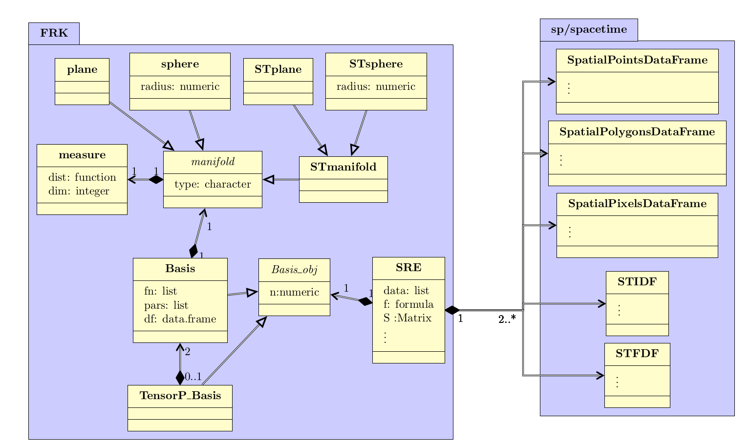
Now, assume that we wish to predict over regions encompassing several BAUs such that the matrix in (11) contains multiple non-zeros per row. We can create this larger regionalisation by using the function \codeauto_BAUs and specifying the cell size. This gives a ‘super-grid’ shown in Figure 6.
R> Pred_regions <- auto_BAUs(manifold = plane(), cellsize = c(600, + 600), type = "grid", data = meuse, convex = -0.05)
We carry out prediction on the super-grid by setting the \codenewdata argument in the function \codepredict, as given below.
R> Pred <- predict(S, newdata = Pred_regions, obs_fs = FALSE)
The predictions and the corresponding prediction standard errors on this super-grid are shown in Figure 6.
3.4 Computational considerations
While FRK beats the curse of ‘data dimensionality’ by dealing with matrices of size instead of matrices of size , one must ensure that the number of basis functions, , remains reasonably small. The reasons are two-fold. First, the computational time required to invert an matrix increases cubicly with , and several such inversions are required when running the EM algorithm. Second, it is likely that more EM-algorithm iterations are required when is large. In practice, should not exceed a few thousand. The number of basis functions can usually be controlled through the argument \codenres. The function \codeauto_basis also takes an argument \codemax_basis that automatically finds the number of resolutions required to not exceed the desired maximum number of basis functions.
The fitting and prediction algorithms scale linearly with the number of data points and the number of BAUs . However, if one has millions of data points, then the number of BAUs must exceed this and a big-memory machine will probably be required. Irrespective of problem size, we have noted considerable improvements in speed when using the OpenBLAS libraries (Wang_2013).
Some of the operations in \pkgFRK can be run in parallel. To use a parallel back-end, one needs to set an option as follows: {Schunk} {Sinput} R> opts_FRK
4 Comparison studies
In this section we compare the utility of the SRE model in \pkgFRK to standard kriging using \pkggstat (Pebesma_2004), and to two other popular models for modelling and predicting with large datasets in \proglangR: the LatticeKrig model that can be implemented with the package \pkgLatticeKrig (LatticeKrig), and the SPDE–GMRF model that can be implemented with the package \pkgINLA (Lindgren_2015). In both these models the spatial field is decomposed as
and is modelled in such a way that it is sparse. These two models allow for feasible computation with large , however neither includes an extra fine-scale effect . The SPDE–GMRF model has the added interpretable feature that, for a given set of basis functions, is such that the resulting field approximates a Gaussian process with a stationary covariance function from the Matérn class.
In Section 4.1, we first analyse a 2D simulated dataset. We shall see that while \pkgFRK may sometimes perform less well in terms of prediction accuracy due to the practical limit on the number of basis functions it uses, it does not under-fit (i.e., it gives valid results) since fine-scale variation is taken into account. In fact, we see that the SRE model in \pkgFRK provides better coverage in terms of prediction intervals, even with large datasets, when compared to other models that use considerably more basis functions but that do not account for fine-scale variation. In the second case study (Section 4.2), we consider three days of column-averaged carbon dioxide data from the Atmospheric InfraRed Sounder instrument on board the Aqua satellite .
4.1 A 2D simulated dataset
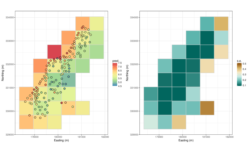
Let , and consider a process with covariance function , where is the marginal variance of the process and is the e-folding length-scale. Further, let be the number of observations and SNR be the signal-to-noise ratio, defined as the ratio of the marginal variance to that of the measurement-error process, . In the inter-comparison, we consider cases where is either or , SNR is 0.2, 1, or 5, and is either 0.015 or 0.15. These choices of parameters help highlight the strengths and weaknesses of FRK with respect to the other approaches. For example, due to the relatively small number of basis functions employed, we expect FRK to have lower prediction precision when the SNR is high and is low, but we expect the prediction intervals to be valid. We further split the domain into two side-by-side partitions, and we placed 95% of the observations in the left half (LH) and 5% in the right half (RH). This partitioning helps identify the different methods’ capability of borrowing strength from a region with dense measurements to a region with sparse measurements. The measurement locations for the case are shown in Figure 7, left panel.
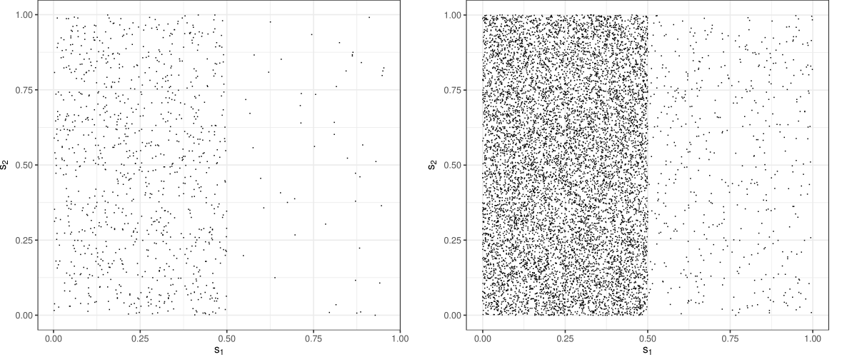
We simulated the process on a 1,000 1,000 grid using the package \pkgRandomFields (Schlather_2015). We used the cells of the grid as our set of BAUs, , and therefore each BAU was of size 0.001 0.001. One such spatial-process realisation for and is shown in Figure 8, left panel, while one with and is shown in Figure 8, right panel. With \pkggstat, which we used to implement simple kriging (denoted gstat), we assumed the true underlying covariance function was known. Hence, when available (for the case), the results of \pkggstat should be taken as the gold standard. As gets larger, simple kriging quickly becomes infeasible, since it is in computational complexity.
We implemented the LatticeKrig model (denoted LTK) using the package \pkgLatticeKrig. We used \codenlevel = 3 resolutions of Wendland basis functions, set the smoothness parameter \codenu = 0.5, and the number of grid points per spatial dimension at the coarsest resolution to \codeNC = 33. The first resolution contained 1,849 basis functions, the second resolution contained 5,625, and the third resolution contained 19,321. In the case where , we set \codefindAwght = TRUE for the effective process range to be estimated by maximum likelihood methods. Setting \codefindAwght = TRUE was prohibitive for , but separate experiments showed that predictions from LTK were largely insensitive to this option for this value of .
We implemented and fit the SPDE–GMRF model (denoted SPDE) using the package \pkgINLA. We constructed a triangular mesh using \codeinla.mesh.2d with \codemax.edge = c(0.05, 0.05) and \codecutoff = 0.012. This gave a mesh with a higher density of basis function on the left-hand side of the domain and (as with the LatticeKrig model) a buffer to reduce edge effects. The basis functions are defined by the triangles, and their number was around 2,500 for , and 5,000 for , while the parameter was used to reproduce Gaussian fields with a Matérn covariance function with smoothness parameter of 1/2 (i.e., an exponential covariance function). Unlike \pkgLatticeKrig and \pkgFRK, \pkgINLA uses an approximate Bayesian method for inference, and thus it requires the specification of prior distributions of the parameters, for which we use penalised complexity priors (Fuglstad_2017). For these simulation settings and our choice of prior distributions, we do not expect the inferential method to be a factor that largely influences the prediction and prediction errors.
For the SRE model implemented in \pkgFRK (denoted FRK) we put a block-exponential covariance structure on (\codeK_type = "block-exponential"), and we set \codenres = 3, yielding, in total, 819 basis functions regularly distributed in the domain . In this study we used \pkgLatticeKrig v6.4, \pkgINLA v17.06.20, and \pkgFRK v0.2.1.
For each configuration in the simulation experiment (i.e., the factorial design defined by and ), we simulated datasets. For prediction locations we took locations at random on the left-hand side of the gridded domain that coincided with measurement locations, and another that did not; and we did the same for the right-hand side. When there were less than 1,000 measurement locations on a given side, all measurement locations were chosen as prediction locations for that side. The sets of locations are denoted as , , , and , respectively. These locations were kept constant across all simulation experiments for a given .
In addition to the stationary, exponential, Gaussian process, we also simulated from the nonstationary process , where
| (14) |
with and . For this additional experiment, we set , , and and we used all configurations in the original experiment as described above. The measurement locations for this case are shown in Figure 7, right panel.
As prediction-performance measures (‘responses’ of the experiment), we considered the following:
-
•
Root mean-squared prediction error: Let denote the ‘model-’ predictor of , where is the th simulated process evaluated at location s and , LTK, SPDE, FRK. Then the model- predictor root-mean-squared prediction error for the th simulation is
(15) where or . Since we are interested in benchmarking the model we use in \pkgFRK, we considered a measure of relative skill (RS), relative to FRK:
where . Hence, indicates that FRK has better (worse) prediction accuracy.
-
•
Ninety-percent coverage: Let denote the prediction variance under model . Then, the ninety-percent coverage, , denotes the percentage of times lies in the interval over . For the 90% coverage measure, is the standard normal’s inverse cumulative distribution function evaluated at , which is 1.64 (rounded to two decimal places). That is,
(16) where , and where .
We intentionally focus on coverage in order to highlight the strengths and weaknesses of the models in terms of uncertainty quantification. Other related measures, such as the Interval Score (Gneiting_2007b), penalise for both prediction interval width and poor coverage and are thus less suited to assess the issue of validity (i.e., whether the prediction intervals are correct, on average). The measures and were considered for simulated from the stationary process with exponential covariance function and from the nonstationary process in (14).
Distributions of for the original experiment with and are shown in Figures 9 and 10, respectively. While it is possible to proceed with an analysis of variance to analyse these results (e.g., Zhuang_2014), here we discuss their most prominent features. First, when there are few () data points (Figure 9), there is little difference between the methods for low SNR but, for high SNR, SPDE and LTK perform better in terms of RS when is small (; see, for example, the bottom left two panels of Figure 9). This was expected since the number of basis functions used begins to play an important role as the SNR increases (Zammit_2018). As expected, all prediction methods perform worse than or as well as, simple kriging with \pkggstat (under a known covariance function).
The comparison in terms of RS is less clear when (Figure 10). First, at unobserved locations, FRK is frequently outperformed in terms of RS by the other methods, since the relatively small number of basis functions is unable to adequately reconstruct the optimal (simple-kriging) predictor. On the other hand, at observed locations, the performance is SNR dependent and data-density dependent. In much of the design space, FRK performs worse (in terms of RS) than the other predictors at the measurement locations, but it begins to outperform SPDE and LTK as the SNR increases and when is small (). Now we turn to the question of ‘validity’ of the predictors.
An equally important performance measure to RMSPE is coverage. Distributions of for and are shown in Figures 11 and 12, respectively. In the small-data case , all methods are over-confident (more so in the left-hand part of the domain) and by varying degrees. In the large-data case , both SPDE and LTK perform poorly in terms of coverage, providing over-confident predictions, especially when the SNR is large (). This is a result of these models relying on basis functions to reproduce the fine-scale variation and not attempting to separate out fine-scale variation from measurement error. The model implemented in \pkgFRK places a white-noise process at the BAU level to capture the fine-scale variation and can thus yield good coverage despite the use of a relatively low-dimensional manifold. It is worth nothing that it is straightforward in \pkgINLA to include an extra fine-scale-variation term and fix the standard deviation of the measurement error to some pre-specified value, although this is rarely done. Here we are illustrating that not doing this may lead to severe deleterious effects on coverage. The model used in \pkgFRK was also found to yield 90% Interval Scores that were at least as good as, or better than, the other two models for the case with (results not shown).
To further investigate this issue, we re-ran the simulations and generated coverage diagnostics for predicted data, , rather than for just . The coverage for all methods was very good (results not shown), indicating that all methods are able to correctly apportion total variability. Consequently, these results show that inclusion of the fine-scale variation term is critical in reduced-rank approaches (irrespective of the number of basis functions) with large datasets when predicting the hidden process. (It is not critical when predicting missing data). The simple semivariogram method employed by \pkgFRK for estimating the measurement-error variance is a step in the right direction, and it appears to yield good results in the first instance. However, ideally, the standard deviation of the measurement error is known from the application and fixed a priori.
Overall, all models have their own relative strengths and weaknesses, largely arising from the differences in (i) the type and number of basis functions employed, and (ii) the presence or otherwise of a fine-scale-process term. In this experiment we saw that the model employed by \pkgFRK produces predictions that are valid, on average. However for large-data situations, our experiment shows FRK predictions to be less efficient, as expected due to the restriction on the number of basis functions that can be used.
In the nonstationary case (14), all methods performed similarly, with LTK being slightly overconfident and FRK being slightly underconfident; see Table 3. This similarity is not surprising since in (14) we set , which results in a process that is highly spatially correlated as well as rather smooth. The resulting process has a similar overall length scale and SNR to that simulated in the original experiment that yielded the results shown in the second row () of the third (LH, ‘10’), fourth (LH, ‘11’), seventh (RH, ‘10’), and eighth (RH, ‘11’) columns of Figures 9 and 11. We see that all three methods performed similarly, and satisfactorily, in this case.
| RMSPE (LH obs) | RMSPE (LH unobs) | RMSPE (RH obs) | RMSPE (RH unobs) | 90% cover. (LH obs) | 90% cover. (LH unobs) | 90% cover. (RH obs) | 90% cover. (RH unobs) | |
| LTK | 0.13 | 0.12 | 0.24 | 0.25 | 0.86 | 0.87 | 0.88 | 0.87 |
| SPDE | 0.13 | 0.12 | 0.24 | 0.25 | 0.90 | 0.89 | 0.91 | 0.88 |
| FRK | 0.13 | 0.13 | 0.24 | 0.25 | 0.92 | 0.92 | 0.91 | 0.91 |
4.2 Modelling and prediction with data from the AIRS instrument
The US National Aeronautics and Space Administration (NASA) launched the Aqua satellite on May 04 2002, with several instruments on board, including the Atmospheric Infrared Sounder (AIRS). AIRS retrieves column-averaged CO2 mole fraction (in units of parts per million), denoted XCO2 (with particular sensitivity in the mid-troposphere), amongst other geophysical quantities (Chahine_2006). The data we shall use consists of XCO2 measurements taken between May 01 2003 and May 03 2003 (inclusive). These data are a subset of those available with \pkgFRK. We compare , and FRK on the three-day AIRS dataset, and we assess the utility of the methods on a validation dataset that we hold out.
Modelling on the sphere with \pkgFRK proceeds in a very similar fashion to the plane, except that a coordinate reference system (CRS) on the surface of the sphere needs to be declared for the data. This is implemented using a \codeCRS object with string \code"+proj=longlat +ellps=sphere". We next outline the six steps required to fit these data using \pkgFRK.
Step 1: Fifteen days of XCO2 data from AIRS (in May 2003) are loaded by using the command \codedata("AIRS_05_2003"). In this case study, we subset the data to include only the first three days, which contains 43,059 observations of XCO2 in parts per million (ppm). We subsequently divide the data into a training dataset of 30,000 observations, chosen at random (\codeAIRS_05_2003_t), and a validation dataset (\codeAIRS_05_2003_v) containing the remaining observations. To instruct \pkgFRK to fit the SRE model on the surface of a sphere, we assign the appropriate \codeCRS object to the data as follows:
R> coordinates(AIRS_05_2003) <- lon + lat R> proj4string(AIRS_05_2003) <- CRS("+proj=longlat +ellps=sphere")
Step 2: The next step is to create BAUs. This is done using the \codeauto_BAUs function but this time with the manifold specified to be the surface of a sphere with radius equal to that of Earth. We also specify that we wish the BAUs to form an ISEA Aperture 3 Hexagon (ISEA3H) discrete global grid (DGG) at resolution 9 (for a total of 186,978 BAUs). Resolutions 0–6 are included with \pkgFRK; higher resolutions are available in the package \pkgdggrids available from \codehttps://github.com/andrewzm/dggrids. By default, this will create a hexagonal grid on the surface of the sphere, however it is also possible to have the more traditional lon-lat grid by specifying \codetype = "grid" and declaring a \codecellsize in units of degrees. An example of an ISEA3H grid, at resolution 5 (which would yield a total of 6,910 BAUs), is shown in Figure 13, left panel, while a lon-lat grid using \codetype = "grid" is shown in Figure 13, right panel.
R> isea3h_sp_poldf <- auto_BAUs(manifold = sphere(), isea3h_res = 9, + type = "hex", data = AIRS_05_2003) R> isea3h_sp_poldf_2_2V_ξ,ZV_δ,Zσ^2_δ= 0σ^2_ξ\VAR(η) = K