Model of a fluxtube with a twisted magnetic field in the stratified solar atmosphere

Abstract

We build a single vertical straight magnetic fluxtube spanning the solar photosphere and the transition region which does not expand with height. We assume that the fluxtube containing twisted magnetic fields is in magnetohydrostatic equilibrium within a realistic stratified atmosphere subject to solar gravity. Incorporating specific forms of current density and gas pressure in the Grad–Shafranov equation, we solve the magnetic flux function, and find it to be separable with a Coulomb wave function in radial direction while the vertical part of the solution decreases exponentially. We employ improved fluxtube boundary conditions and take a realistic ambient external pressure for the photosphere to transition region, to derive a family of solutions for reasonable values of the fluxtube radius and magnetic field strength at the base of the axis that are the free parameters in our model. We find that our model estimates are consistent with the magnetic field strength and the radii of Magnetic bright points (MBPs) as estimated from observations. We also derive thermodynamic quantities inside the fluxtube.

1 Introduction

The study of small scale magnetic structures in the solar photosphere is important because they play a crucial role in the evolution of active regions and sunspots (Muller and Mena, 1987; Centeno et al., 2007). Magnetic bright points (MBPs) are likely to be the fluxtubes observed in the photosphere (Berger et al., 1995; Centeno et al., 2007; Lagg et al., 2010). The topological rearrangement of these magnetic fluxtubes due to the motion of the photospheric foot points or magnetic reconnections, contribute to the coronal heating (Muller et al., 1994; van Ballegooijen, 1986). A three dimensional (3D) single fluxtube model with untwisted magnetic field has been studied by solving linear elliptic partial differential equation by numerical iterative process (Steiner et al., 1986). Schlüter and Temesváry (1958) and Osherovich (1984) studied a 3D fluxtube for sunspots using a self–similar model. The magnetic and thermodynamic structure inside fluxtube with untwisted magnetic field which spans from photosphere to the lower part of the solar corona is studied by Gent et al. (2013). Both 2D and 3D numerical models of fluxtubes with the energy propagation through the torsional Alfven waves have been studied by Murawski et al. (2015a, b), where an empirical form of magnetic flux function was assumed. Vigeesh et al. (2009) assumed an empirical form of gas pressure to investigate the wave propagation and energy transport through a fluxtube. Several interesting results of wave behavior in the solar photosphere and chromosphere have been presented by several authors (Bogdan et al., 2003; Fedun et al., 2009; Shelyag et al., 2010).
In this work, we construct a 3D single cylindrical vertical straight magnetic fluxtube semi-analytically with a twisted magnetic field by obtaining a new solution of poloidal flux function by solving Grad–Shafranov equation (GSE; Grad and Rubin (1958); Shafranov (1958)). We assume a specific form of gas pressure and poloidal current, which has been used to study the equilibrium solution of terrestrial plasma (Atanasiu et al., 2004). An equilibrium solution near the magnetic axis of the plasma torus has been reported previously, using a plasma pressure and poloidal current profile that varies linearly with the poloidal flux function (Solov’ev, 1968). We obtain an analytic solution by assuming a form that is quadratic in the poloidal flux function, and derive the magnetic field structure and thermodynamic quantities inside the fluxtube using the solution that represents an ideal MHS equilibrium. In the future, we will look to explore fully the profile functions that will improve the solution set.
The overview of the paper is as follows. In section 2, the GSE has been derived assuming a specific form of the profile function of gas pressure and poloidal current and the solution of the equation is presented. In section 3, we discuss the boundary condition that is physically acceptable, and can be used for realistic modelling of a fluxtube. In section 4, the mode wise variation of the profile functions are presented and in section 5, we compare the model with the observations. Finally, we conclude with a comparison with other existing models.

2 Solution of Grad-Shafranov equation

We assume an axisymmetric cylindrical geometry, with gas pressure $p$ and take the poloidal current $I_{p}$ constant along a magnetic field line. We express $p(\Psi,z)$ and $I_{p}(\Psi)$ in terms of the poloidal flux function $\Psi(r,z)$ and $z$ and consider a straight vertical axisymmetric fluxtube that spans the altitude from photosphere ($z=0$) to the transition region ($z=2.15$ Mm) that is in equilibrium with the atmosphere outside with the uniform gravity ${\bf g}(=-g\hat{z})$ acting vertically downward. The force balance equation in MHS equilibrium takes the form

$$-\nabla p+\frac{1}{4\pi}(\nabla\times{\bf B})\times{\bf B}+\rho{\bf g}=0,$$ (1)

where $\rho$ denotes the mass density and ${\bf B}$ is the magnetic field associated with the poloidal flux function $\displaystyle{\Psi(r,z)=\int_{0}^{r}B_{z}(r^{\prime},z)r^{\prime}{\rm d}r^{\prime}}$ (scaled by the factor $\frac{1}{2\pi}$) in the following form

$$B_{r}=-\frac{1}{r}\frac{\partial\Psi}{\partial z};\quad B_{z}=\frac{1}{r}\frac{\partial\Psi}{\partial r};\quad B_{\phi}=\frac{I_{p}}{r}.$$ (2)

This form of $B_{r},B_{\phi}$ and $B_{z}$ ensures the solenoidal condition of magnetic field. Now splitting the MHS force balance equation (1) into $r$ and $z$ directions, we find two different scalar partial differential equations

$$-\frac{\partial p}{\partial r}+\frac{1}{4\pi}\bigg{(}B_{r}\frac{\partial B_{r}}{\partial r}+B_{z}\frac{\partial B_{r}}{\partial z}-\frac{1}{2}\frac{\partial B^{2}}{\partial r}\bigg{)}=0$$ (3a)

$$-\frac{\partial p}{\partial z}+\frac{1}{4\pi}\bigg{[}\frac{1}{r}\frac{\partial\Psi}{\partial z}\bigg{(}\frac{1}{r^{2}}\frac{\partial\Psi}{\partial r}-\frac{1}{r}\frac{\partial^{2}\Psi}{\partial r^{2}}\bigg{)}-\frac{1}{r^{2}}\frac{\partial\Psi}{\partial z}\frac{\partial^{2}\Psi}{\partial z^{2}}-\frac{1}{2r^{2}}\frac{\partial}{\partial z}(I_{p}^{2})\bigg{]}-\rho g=0.$$ (3b)

If the gas pressure and poloidal current are functions of $\Psi$ alone i.e., $p_{1}(\Psi)$ and $I_{p}(\Psi)$ respectively, then from the (3a, 2) it follows that

$$\frac{\partial^{2}\Psi}{\partial r^{2}}-\frac{1}{r}\frac{\partial\Psi}{\partial r}+\frac{\partial^{2}\Psi}{\partial z^{2}}=-\frac{1}{2}\frac{\partial I_{p}^{2}(\Psi)}{\partial\Psi}-4\pi r^{2}\frac{\partial p_{1}(\Psi)}{\partial\Psi}.$$ (4)

Plugging in $p_{1}$ and $I_{p}^{2}$ in (3b), we find

$$-\frac{\partial p_{1}(\Psi)}{\partial z}+\frac{1}{4\pi}\bigg{[}\frac{1}{r^{2}}\frac{\partial\Psi}{\partial z}\bigg{(}\frac{1}{r}\frac{\partial\Psi}{\partial r}-\frac{\partial^{2}\Psi}{\partial r^{2}}\bigg{)}-\frac{1}{r^{2}}\frac{\partial\Psi}{\partial z}\frac{\partial^{2}\Psi}{\partial z^{2}}-\frac{1}{2r^{2}}\frac{\partial I_{p}^{2}(\Psi)}{\partial z}\bigg{]}-\rho g=0.$$ (5)

By multiplying both sides of (5) by $\displaystyle{4\pi r^{2}\frac{\partial z}{\partial\Psi}}$ and using (4), we obtain $\displaystyle{g\rho\frac{\partial z}{\partial\Psi}=0}$ which implies that $\rho$ is zero, which means that the vertical hydrostatic pressure balance will not be maintained. Therefore, to balance the vertical hydrostatic pressure inside the fluxtube, we introduce a new function, $p_{2}(z)$ such that,

$$p(r,z)=p_{1}(\Psi)+p_{2}(z).$$

We assume $p_{1}(\Psi)$ and $I_{p}^{2}(\Psi)$ to be second order polynomials of $\Psi$

$$p(r,z)=p_{1}(\Psi)+p_{2}(z)$$ (6a)

$$I_{p}^{2}(r,z)=\tilde{\alpha}\Psi^{2}+\tilde{\beta}\Psi+I_{0}^{2}$$ (6b)

where

$$p_{1}(\Psi)=\tilde{a}\Psi^{2}+\tilde{b}\Psi,$$

and the parameters $\tilde{a},\tilde{b},\tilde{\alpha},\tilde{\beta}$ and $I_{0}^{2}$ are to be determined by appropriate boundary conditions. The function $p_{2}(z)$ is to be evaluated later. The substitution of $p$ given by (6a) in (3a) gives (4) and we obtain the following second order scalar partial linear inhomogeneous differential equation

$$\frac{\partial^{2}\Psi}{\partial r^{2}}-\frac{1}{r}\frac{\partial\Psi}{\partial r}+\frac{\partial^{2}\Psi}{\partial z^{2}}=-(ar^{2}+\alpha)\Psi-(br^{2}+\beta),$$ (7)

with the rescaled parameters, $\displaystyle{a=8\pi\tilde{a};\alpha=\tilde{\alpha};b=4\pi\tilde{b};\beta=\tilde{\beta}/2}$. To solve (7), we split $\Psi$ in two parts: a homogeneous part, $\Psi_{h}(r,z)$ and an inhomogeneous part $\Psi_{p}(r)$, i.e. $\Psi(r,z)=\Psi_{h}(r,z)+\Psi_{p}(r)$. Using this form in (7), we separate the homogeneous and the inhomogeneous parts to obtain the following expressions:

$$\frac{\partial^{2}\Psi_{h}}{\partial r^{2}}-\frac{1}{r}\frac{\partial\Psi_{h}}{\partial r}+\frac{\partial^{2}\Psi_{h}}{\partial z^{2}}=-(ar^{2}+\alpha)\Psi_{h}$$ (8a)

$$\frac{\partial^{2}\Psi_{p}}{\partial r^{2}}-\frac{1}{r}\frac{\partial\Psi_{p}}{\partial r}=-(ar^{2}+\alpha)\Psi_{p}-(br^{2}+\beta).$$ (8b)

To solve the homogeneous part, we seek a solution of the form $\Psi_{h}(r,z)=S(r)Z(z)$. Then we separate out the $r$ and $z$ part in (8a) as follows

$$\frac{S^{\prime\prime}}{S}-\frac{1}{r}\frac{S^{\prime}}{S}+ar^{2}+\alpha=-\frac{Z^{\prime\prime}}{Z}=-k^{2},$$ (9)

where $k$ is an arbitrary real constant. Motivated by the fact that the poloidal flux function $\Psi(r,z)$ decreases with $z$, we assume that the solution of the $z$-part of (9) takes the form

$$Z(z)=Ce^{-kz},$$ (10)

where $C$ is an arbitrary constant. To solve the $r$–part of (9), we substitute $x=\frac{\sqrt{a}r^{2}}{2}$ (where $a>0$) and insert it in (9) to find

$$\frac{{\rm d}^{2}S}{{\rm d}x^{2}}+\bigg{(}1+\frac{2\eta}{x}\bigg{)}S=0,$$ (11)

whose solutions are given by Coulomb wave functions $F_{L}(-\eta,x)$ and $G_{L}(-\eta,x)$ (Abramowitz and Stegun, 1972) (page $537-544$) with $L=0$ and $\displaystyle{\eta=\frac{\alpha+k^{2}}{4\sqrt{a}}}$. The solution of (11) takes the following form

$$S(r)=C_{1}F_{0}\big{(}-\eta,\frac{\sqrt{a}r^{2}}{2}\big{)}+C_{2}G_{0}\big{(}-\eta,\frac{\sqrt{a}r^{2}}{2}\big{)}.$$ (12)

Here $F_{0}\big{(}-\eta,\frac{\sqrt{a}r^{2}}{2}\big{)}$ and $G_{0}\big{(}-\eta,\frac{\sqrt{a}r^{2}}{2}\big{)}$ are called the regular and irregular Coulomb wave functions respectively which are complex quantities with real arguments (Boersma, 1968), given by

$$F_{0}(-\eta,\frac{\sqrt{a}r^{2}}{2})=C_{0}(\eta)M_{-i\eta,1/2}(i\sqrt{a}r^{2}),$$ (13)

$$G_{0}(-\eta,\frac{\sqrt{a}r^{2}}{2})=iC_{0}(\eta)M_{-i\eta,1/2}(i\sqrt{a}r^{2})+D_{0}(\eta)W_{-i\eta,1/2}(i\sqrt{a}r^{2}),$$ (14)

where $M_{-i\eta,1/2}(i\sqrt{a}r^{2})$ and $W_{-i\eta,1/2}(i\sqrt{a}r^{2})$ are called the Whittaker-M and Whittaker-W function (see Figure 3 below) and the constants $C_{0}(\eta)$ and $D_{0}(\eta)$ are defined by

$$C_{0}(\eta)=\frac{1}{2}|\Gamma(1-i\eta)|e^{-\frac{\pi}{2}(i-\eta)}$$ (15)

and

$$D_{0}(\eta)=\frac{\Gamma(1-i\eta)}{|\Gamma(1-i\eta)|}e^{-\frac{\pi\eta}{2}}.$$ (16)

The Whittaker function has been used by several authors in their models of the solar atmosphere albeit in different physical problems (eg. Tsinganos (1979) in the context of inviscid flows, and also in the context of MHD waves by Hindman and Jain (2008) and Erdélyi and Fedun (2010)). Now $B_{z}(r,z)$ has to be a finite quantity that varies linearly with the term $\displaystyle{\frac{1}{r}\frac{\mathrm{d}S}{\mathrm{d}r}}$ but $\displaystyle{\frac{1}{r}\frac{\mathrm{d}}{\mathrm{d}r}[G_{0}(-\eta,\frac{\sqrt{a}r^{2}}{2})]}$ blows up at $r=0$; therefore for $B_{z}$ to be finite on the axis of the fluxtube $C_{2}$ in (12) must vanish. As a result $S(r)$ takes the form

$$S(r)=C_{1}F_{0}\big{(}-\eta,\frac{\sqrt{a}r^{2}}{2}\big{)},$$ (17)

and the homogeneous part of the solution is given by

$$\Psi_{h}(r,z)=Ce^{-kz}F_{0}\big{(}-\eta,\frac{\sqrt{a}r^{2}}{2}\big{)}.$$ (18)

A similar but a different solution, which is oscillatory in $z$ is used for laboratory plasma for both a $D$-shaped plasma and toroidally diverted plasma (Atanasiu et al., 2004). The general solution of (7) is given by the sum of the homogeneous part $\Psi_{h}(r,z)$ given above and an inhomogeneous part $\Psi_{p}(r)$ which will be presented in a paper in preparation. We have found that the presence of $\Psi_{p}(r)$ term in the poloidal flux function $\Psi(r,z)$, implies that $p$ and $I_{p}^{2}$ cannot be simultaneously positive for any combination of $b$ and $\beta$ in the physical parameter domain space for all $r$ and $z$. For avoiding these unphysical effects we present the case of $\Psi=\Psi_{h}$ and an exploration of the general solution $\Psi=\Psi_{h}+\Psi_{p}$ will be studied later. Since $\Psi(r,z)$ and its complex conjugate function, $\Psi^{*}(r,z)$ are the valid solutions of (7), we construct a solution of (7) by redefining $\displaystyle{\frac{\Psi(r,z)+\Psi^{*}(r,z)}{2}\rightarrow\Psi(r,z)}\equiv\varsigma(r)Z(z)$.

3 Boundary conditions and the reduced form of $p$ and $I_{p}$

The ideal magnetic fluxtube is embedded in a magnetic field free region with no current outside the fluxtube boundary. We make the following standard assumptions $B_{r}(r=R,z)=0$ and $B_{\phi}(r=R,z)=0$ to ensure that there is no net current $I_{p}$ at the fluxtube boundary. The pressure at the photosphere ($z=0$) outside the fluxtube is $p_{0}=1.228\times 10^{5}$ dyne cm^-2 and at the transition region ($z_{tr}=2.15$ Mm) is $p_{tr}=0.1058$ dyne cm^-2 and is taken from Avrett-Loeser model (Avrett and Loeser, 2008). We summarize the boundary conditions below

$$B_{r}(R,z)=0$$ (19a)

$$B_{\phi}(R,z)=0$$ (19b)

$$p(R,0)=p_{0}$$ (19c)

$$p(R,z_{tr})=p_{tr}$$ (19d)

Assuming that pressure decreases exponentially from photosphere to transition region, we use the following expression for the external pressure

$$p_{ex}(z)=p_{0}\exp(-2kz),$$ (20)

where $\displaystyle{k=\frac{1}{2\times 2.15}\ln\big{(}\frac{p_{0}}{p_{tr}}\big{)}}$ Mm${}^{-1}=3.248$ Mm${}^{-1}.$ Matching the pressure scale heights, we see that $p_{2}(z)$ (6a) also decreases exponentially with $z$ as

$$p_{2}(z)=p_{20}\exp(-2kz),$$ (21)

where $p_{20}$ will need to be calculated. Taking $\Psi(r,z)=\Psi_{h}(r,z),$ the reduced forms of $p$ and $I_{p}^{2}$ are given by

$$p(\Psi,z) =\frac{a}{8\pi}\Psi^{2}+p_{2}(z)\quad(a>0)$$ (22)

and

$$I_{p}^{2}(\Psi) =\alpha\Psi^{2}\quad(\alpha>0).$$ (23)

Taking the radial component of the MHS force balance equation (1) and adding the contribution of the radial force due to the presence of sheet current $j_{\phi}$ at the boundary we write the force balance equation

$$-\frac{\partial p}{\partial r}\bigg{|}_{r=R}+\frac{1}{4\pi}\bigg{(}B_{r}\frac{\partial B_{r}}{\partial r}+B_{z}\frac{\partial B_{r}}{\partial z}\bigg{)}\bigg{|}_{r=R}-\frac{\partial}{\partial r}\bigg{(}\frac{B^{2}}{8\pi}\bigg{)}\bigg{|}_{r=R}+j_{\phi}(r)B_{z}(r)\bigg{|}_{r=R}=0.$$ (24)

Now the sheet current $j_{\phi}$ can be expressed as a delta function $j_{\phi}(r)=j_{\phi s}\delta(r-R)$ which is non zero only at the boundary. Integrating (24) w.r.t. $r$ from $r=R-\epsilon$ to $r=R+\epsilon$ where $\epsilon$ is an infinitesimal positive quantity we obtain

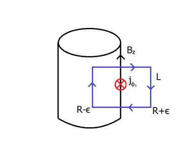
Figure 1: Fluxtube geometry at the boundary showing the sheet current.

$$-\int_{R-\epsilon}^{R+\epsilon}\frac{\partial p}{\partial r}dr+\frac{1}{4\pi}\bigg{(}\int_{R-\epsilon}^{R+\epsilon}B_{r}\frac{\partial B_{r}}{\partial r}dr+\int_{R-\epsilon}^{R+\epsilon}B_{z}\frac{\partial B_{r}}{\partial z}dr\bigg{)}$$ (25)

$$-\int_{R-\epsilon}^{R+\epsilon}\frac{\partial}{\partial r}\bigg{(}\frac{B^{2}}{8\pi}\bigg{)}dr+\int_{R-\epsilon}^{R+\epsilon}j_{\phi}(r)B_{z}(r){\rm d}r=0,$$

which leads to the MHS force balance at the boundary to be given by

$$p_{in}-p_{ex}+j_{\phi s}B_{z}(R)+\frac{1}{4\pi}\bigg{[}B_{r}\frac{\partial B_{r}}{\partial r}+B_{z}\frac{\partial B_{r}}{\partial z}\bigg{]}_{R}+\frac{B_{i}^{2}-B_{e}^{2}}{8\pi}=0,$$ (26)

where $[...]_{R}$ denotes the jump condition at the boundary and $B_{i}$ and $B_{e}$ are the magnetic fields inside and outside the fluxtube boundary. This is an improved boundary pressure condition for a magnetic fluxtube, as previous studies have ignored the sheet current. Now to calculate $j_{\phi s}$, we assume an infinitesimal current loop at the boundary which has a vertical height of length $L$ and radial extent from $R-\epsilon$ to $R+\epsilon$. Using Stokes line integral theorem along the closed loop (see Fig.1), we see that

$$B_{z}L=4\pi L\int_{R-\epsilon}^{R+\epsilon}j_{\phi s}\delta(r-R){\rm d}r,$$ (27)

which implies $\displaystyle{j_{\phi s}=\frac{B_{z}}{4\pi}}$. Since $B_{r}(R)=B_{\phi}(R)=B_{e}(R)=0$ for any height $z$ and $p_{in}(R,z)=p_{2}(z)$, from (26), the total pressure at the boundary inside the fluxtube is $\displaystyle{p_{2}(z)+\frac{3B_{z}^{2}(R)}{8\pi}}$ and matching the pressures gives

$$p_{2}(z)=p_{ex}(z)-\frac{3B_{z}^{2}(R,z)}{8\pi}.$$ (28)

The mass density inside the fluxtube obtained from (3b) is

$$\rho(z)=-\frac{1}{g}\frac{\mathrm{d}p_{2}(z)}{\mathrm{d}z},$$ (29)

and the density inside the fluxtube varies only with $z$ and at the transition region ($z_{tr}=2.15$ Mm), which should match with the external density which is typically $\rho_{tr}=2.77\times 10^{-14}$ g cm^-3 (Avrett and Loeser, 2008). From (28) and (20) we see that

$$p_{20}=\frac{g}{2k}e^{2kz_{tr}}\rho_{tr}.$$ (30)

In our model $g$ is assumed not to vary much from photosphere to the transition region and its value is taken to be $g=274$ m s^-2, the value at the solar surface and that determines $p_{20}=1.36\times 10^{4}$ dyne cm^-2. Using the forms of $B_{z}(r,z)$ from (2, 18) we obtain $B_{z}(0,0)=4\sqrt{a}C\equiv B_{z0}$, and the relation between $C,B_{z0}$ and $a$ is derived in the following.
The real component of $\Psi$ is given by,

$${\rm Re}(\Psi)=\frac{\Psi+\Psi*}{2}$$

and by using (13) and (18) we can express the flux function in the form of Whittaker–M functions as

$$\Psi(r,z)=Ce^{-kz}\bigg{[}M_{-i\eta,1/2}(i\sqrt{a}r^{2})+M_{i\eta,1/2}(-i\sqrt{a}r^{2})\bigg{]}.$$ (31)

Whittaker–M function can be expressed in terms of hypergeometric function by the standard relation (Dixit and Moll, 2015)

$$M_{t,m}(z)=e^{-z/2}z^{m+1/2}F_{1}^{1}(1/2+m-t,1+2m,z).$$ (32)

Here $F_{1}^{1}$ represents the hypergeometric functions with the parameters $t,m$ and argument $z$. Therefore (31) takes the form

$$\Psi(r,z)=Ce^{-kz}\sqrt{a}r^{2}\bigg{[}e^{-i\sqrt{a}r^{2}/2}F_{1}^{1}(1+i\eta,2,i\sqrt{a}r^{2})+e^{i\sqrt{a}r^{2}/2}F_{1}^{1}(1-i\eta,2,-i\sqrt{a}r^{2})\bigg{]}.$$ (33)

It follows from (2) that $B_{z}$ takes the form

$$B_{z}(r,z)=\frac{\sqrt{a}C}{2}e^{-kz}e^{-i\sqrt{a}r^{2}/2}\bigg{[}(8+4i\sqrt{a}r^{2})F_{1}^{1}\bigg{(}\frac{4\sqrt{a}+i(k^{2}+\alpha)}{4\sqrt{a}},2,i\sqrt{a}r^{2}\bigg{)}-$$ (34)

$$r^{2}(4i\sqrt{a}+k^{2}+\alpha)F_{1}^{1}\bigg{(}\frac{4\sqrt{a}+i(k^{2}+\alpha)}{4\sqrt{a}},3,i\sqrt{a}r^{2}\bigg{)}\bigg{]}.$$

So, $B_{z}(r,z)$ at $r=z=0$ is by definition $B_{z0}$ takes the form from (34) as,

$$B_{z0}=4\sqrt{a}CF_{1}^{1}\bigg{(}\frac{4\sqrt{a}+i(k^{2}+\alpha)}{4\sqrt{a}},2,0\bigg{)}.$$ (35)

But $F_{1}^{1}\bigg{(}\frac{4\sqrt{a}+i(k^{2}+\alpha)}{4\sqrt{a}},2,0\bigg{)}=1$ is an identity and therefore we finally have

$$C=\frac{B_{z0}}{4\sqrt{a}}.$$ (36)

We define a physical observable $B_{0}$ which is the average magnetic field strength at the base within the fluxtube as

$$B_{0}=\frac{1}{R}\int_{0}^{R}\sqrt{B_{r}^{2}(r,0)+B_{z}^{2}(r,0)+B_{\phi}^{2}(r,0)}{\rm d}r$$ (37)

where $R$ is the radius of the fluxtube. Therefore we have two free parameters $R$ and $B_{0}$ that we can tune to fit our model with the observations. At $z=0$, from (28), we get

$$\frac{3B_{z}^{2}(R,0)}{8\pi}=p_{0}-p_{20}.$$ (38)

Therefore, from (19a, 19b, 19c) we determine $a$, $\alpha$ and $C$ in terms of the free parameters $R$ and $B_{0}$ and hence the thermodynamic quantities within fluxtube. The temperature within the fluxtube is calculated by the ideal gas law according to the following form

$$T(r,z)=\frac{\bar{\mu}p(r,z)}{\rho(z)R_{g}},$$ (39)

where $R_{g}=8.314$ J mol^-1 K^-1 is the universal gas constant and

$$\bar{\mu}=\frac{1}{z_{max}}\int_{0}^{z_{max}}\mu_{eff}(z)\mathrm{d}z=1.116,$$

is the average value of the mean effective molar mass from photosphere to transition region given by an empirical formula $\displaystyle{\mu_{eff}(z)=1.288\big{[}1-0.535\big{(}\frac{z}{2.152}\big{)}^{3}\big{]}}$ (Solov’ev and Kirichek, 2015) in the domain of $0<z<2.152$ Mm. A formulary of the different quantities are listed in Table 1.

Functions	$r$–part	$z$–part
$\Psi(r,z)$	$\varsigma(r)$	$Z(z)$
$B_{r}(r,z)$	$\frac{3.248\times 10^{-8}}{r}\varsigma(r)$	$Z(z)$
$B_{\phi}(r,z)$	$\sqrt{\alpha}\frac{\varsigma(r)}{r}$	$Z(z)$
$B_{z}(r,z)$	$\frac{\varsigma^{\prime}(r)}{r}$	$Z(z)$
$p(r,z)$	$\frac{a}{8\pi}\varsigma^{2}(r)+p_{20}$	$Z^{2}(z)$
$\rho(r,z)$	$1$	$(3.22\times 10^{-8})Z^{2}(z)$
$T(r,z)$	$0.0416\big{(}\frac{a}{8\pi}\varsigma^{2}(r)+p_{20}\big{)}$	1

Table 1: A formulary of the derived functions obtained from the solution of GSE. Here, $\varsigma(r)=C\big{[}F_{0}\big{(}-\eta,\frac{\sqrt{a}r^{2}}{2}\big{)}+F^{*}_{0}\big{(}-\eta,\frac{\sqrt{a}r^{2}}{2}\big{)}\big{]}$ and $Z(z)=e^{-kz}$. The value of the constants are $\bar{\mu}=1.116$, $g=2.74\times 10^{4}$ cm s^-2, $k=3.248\times 10^{-8}$ cm^-1, $p_{20}=1.36\times 10^{4}$ dyne cm${}^{-2}.$ All the quantities in the table are in cgs units.

4 Mode analysis of different profile functions

The quantities $a,\alpha$ and $C$ are functions of the free parameters $R$, $B_{0}$ and the mode number $n$ whose values are given in Table 2 for a sample set of the free parameters.

$R$ (km)	$B_{0}$ (kG)	mode no.	C ($10^{17}$ Mx)	$\alpha$ ($10^{-14}$ cm-2)	a ($10^{-28}$ cm-4)
100	1	1	0.335061	7.50448	20.0417
100	1	2	0.144828	15.6546	107.27
100	1	3	0.0915463	24.0161	268.473

Table 2: Values of the quantities $a,\alpha$ and $C$ for $R=100$ km and $B_{0}=1$ kG for three different modes.

The solutions to $\Psi,B,p$ and $T$ are shown for different mode numbers, in Figs. 2–5 respectively.

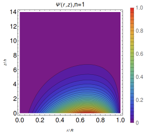
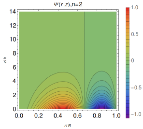
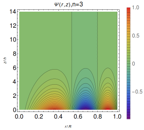
Figure 2: The vertical cross–sections of normalized poloidal flux function for three different modes $n$ for $R=100$ km and $B_{0}=1$ kG are shown. The contours represent the magnetic lines of force in the $r-z$ plane. The amplitude of the flux function, normalized to the peak value, is represented by a colour bar. The horizontal axis is scaled to the radius of the fluxtube $R$ and the vertical axis is scaled with the pressure scale height, $h=162$ km.

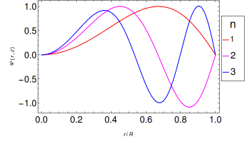
Figure 3: The radial variations of the normalized poloidal flux function for three different modes for $R=100$ km and $B_{0}=1$ kG are shown.

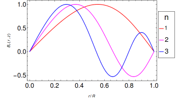
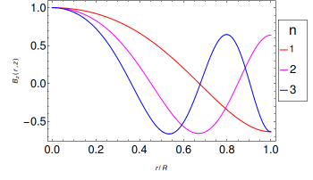
Figure 4: The radial variations of the normalized $B_{r}$, $B_{\phi}$ and $B_{z}$ fields for different modes for $R=100$ km and $B_{0}=1$ kG are shown.

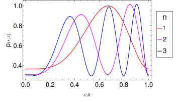
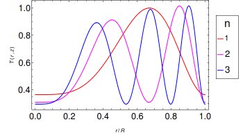
Figure 5: Left: The radial variations of normalized gas pressure within the fluxtube are shown for three different modes $n$, Right: The radial variations of normalized temperature profile inside the fluxtube are shown for three different modes $n$. Both the plots are for $R=100$ km and $B_{0}=1$ kG.

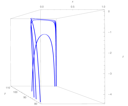
Figure 9: The figure shows the $3$D topology of the magnetic field lines inside the fluxtube. The scales are in arbitrary units.

All the profile functions are normalized to their peak values and the radial distance to the total radius of the fluxtube $R$. As per the boundary conditions, the flux function, $\Psi$ vanishes both at the axis and at the boundary of the fluxtube, where the the total gas pressure is $p_{2}(z)$. The solutions of higher modes have, the profile functions with higher frequency along the radial direction and realistically we may not have such reversible fields, as they are unstable. Therefore, we use the fundamental mode ($n=1$) for further analysis in the paper. The $3$D topology of the magnetic field lines inside the fluxtube for the fundamental mode is shown in Fig. 9.

5 Comparing the model with observations

Now we compare our model with the observations reported from high resolution and high cadence instruments. Small scale magnetic structures, i.e., MBPs, are the best candidates for comparison because such structures can be assumed to consist of fluxtubes. MBPs are seen in G-band filtergrams or are identified by making spectro-polarimetric measurements (Utz et al., 2009, 2013; Yang et al., 2016). The radial variation of the profile functions $p,\rho$ and $T$ and the magnetic components $B_{r},B_{\phi}$ and $B_{z}$ are independent of $z$, but the amplitude decreases exponentially with $z$ except for $T$. In the following, we validate the model by comparing the observed magnetic field strengths and radius of MBPs with those calculated in our model, and estimate the magnetic field strength and thermodynamic quantities at the transition region which may be verified by future observations.

The MBPs number distribution, magnetic field strength and size distribution has been reported by Utz et al. (2009, 2013) at photosphere. The size distribution of MBPs peaks around $200$ km and $160$ km for low and high spatial sampling rates, respectively (Utz et al., 2009). The magnetic field strength distribution is bimodal with two peaks at $\sim 1400$ G and $\sim 200$ G (Utz et al., 2013). Since MBPs are observed as the region of unipolar flux concentrations, we construct a cylindrical boundary inside the simulation domain where the vertical magnetic field $B_{z}$ is positive. We call this cut–off radius as $r_{0}$, where the line of sight magnetic field $B_{z}$ vanishes. The value of $B_{z}$ after this grid line becomes negative. In Fig. 6, the vertical grid line denotes the boundary radius $r_{0}$. We study two different cases for $r_{0}=80$ and $100$ km which corresponds to the peak values for the MBP size distribution, for which $R$ is found to be $127$ and $159$ km respectively.

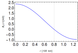
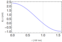
Figure 6: The radial variations of the magnetic field strength at the photosphere ($z=0$) within the fluxtube for $R=127$ km (top) and $159$ km (bottom) are shown. The vertical grid line denotes the radius ($r_{0}$) beyond which $B_{z}$ becomes negative. The values of $r_{0}$ are $80$ km and $100$ km for the top and bottom panels respectively. The horizontal axes are scaled in units of $100$ km and the vertical axes are scaled in units of kG for both top and bottom panels. The mean value of $B_{z}$ up to $r_{0}$ is $1.42$ kG in both panels.

For both cases, we calculate $B_{0}$ and the mean value of $B_{z}$, $\bar{B_{z}}$ in the radial direction up to $r_{0}$ and find that for realistic values of the thermodynamic quantities inside the fluxtube, the upper limit of the vertical magnetic field strength $B_{z0}$ is $2.37$ kG. Beyond this value of $B_{z0}$, the viable solutions will shift to the higher modes. The temperature inside the fluxtube increases as the value of $B_{z0}$ decreases and temperature inside the fluxtube becomes greater than the typical photospheric temperature when $B_{z0}<2.31$ kG. Thus it can be considered as the lower cut off limit of the magnetic field strength. The $\bar{B_{z}}$ value is only sensitive to $B_{z0}$ but not on $r_{0}$, and the thermodynamic quantities inside the fluxtube remain the same for both $r_{0}=80$ and $100$ km. We found $\bar{B_{z}}=1.42$ and $1.4$ kG for $B_{z0}=2.37$ and $2.31$ kG respectively. The radial and vertical variations of the vertical magnetic field strength, gas pressure, density and temperature inside the fluxtube are shown in Figs. 7 and 8. We see that the vertical magnetic field strength decreases from $2.37$ kG (on the axis at $z=0$) to zero at the MBP boundary ($r_{0}$, see Fig. 6). The variation of gas pressure and temperature from axis to the MBP boundary is very small; at the photosphere the gas pressure changes $1.358\times 10^{4}$ (on the axis at $z=0$) to $1.373\times 10^{4}$ dyne cm^-2 (at MBP boundary) and it decreases with $z$ to $3.12\times 10^{-2}$ dyne cm^-2 (at MBP boundary) at the transition region ($z=2$ Mm). The temperature changes from $5656$ K (on the axis) to $5718$ K (at MBP boundary) which is small compared to the outside photosphere temperature ($6583$ K) (Avrett and Loeser, 2008). The average temperature inside fluxtube has been calculated by integrating the temperature from axis to the MBP boundary and is found to be $5679$ K. The density distribution is constant along the radius of the fluxtube at a given height which decreases with height from $3.22\times 10^{-8}$ g cm^-3 at the photosphere to $7.33\times 10^{-14}$ g cm^-3 at the transition region. The values of the quantities estimated from our modelled are summarized in Table 3.

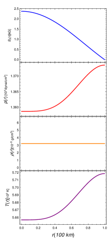
Figure 7: From top to bottom: Predicted radial variation of vertical magnetic field strength, gas pressure, density and temperature from the axis to the boundary of the fluxtube for two different sizes of MBPs ($80$ km radius in the left panel and $100$ km radius in the right panel). The horizontal axis is scaled in units of $100$ km and the vertical axes of $B_{z},p,\rho,T$ are scaled in units of kG, $10^{4}$ dyne cm^-2, $10^{-8}$ g cm^-3 and $10^{3}$ K respectively.

Figure 8: The figure shows the variation of gas pressure, density and temperature at the BP boundary along $z$. The horizontal axis represents the height from the photosphere scaled with the pressure scale height $h=162$ km, and the vertical axes represents pressure, density and temperature from top to bottom respectively.

$r$	$z$ (Mm)	$B_{z}$ (G)	$p$ (dyne cm-2)	$\rho$ (g cm-3)	$T$ (K)
0	0	2370	$1.358\times 10^{4}$	$3.22\times 10^{-8}$	5656
0	2	2.19	$3.09\times 10^{-2}$	$7.33\times 10^{-14}$	5656
$r_{0}$	0	0	$1.373\times 10^{4}$	$3.22\times 10^{-8}$	5718
$r_{0}$	2	0	$3.12\times 10^{-2}$	$7.33\times 10^{-14}$	5718

Table 3: Table of the results obtained from our model for $r_{0}=80$ and $100$ km

6 Conclusions and discussion

In this paper, we constructed a single fluxtube with twisted magnetic field by solving GSE analytically. We summarize our results below:

1. We have an improved boundary condition by incorporating the sheet current as compared to the previous studies e.g. Solov’ev and Kirichek (2016).

2. Our model depends on the form of the external pressure distribution which is assumed as an exponentially decreasing function with $z$. Future observations leading to the more accurate form of pressure distribution from photosphere to transition region can be used to improve our model. The plasma $\beta$ parameter inside the fluxtube remains constant with $z$ but it varies along $r$; $\beta<1$ is obeyed from the chromosphere to the transition region but not in the photosphere and lower atmosphere. Therefore the magnetic effects will dominate the gas dynamics throughout the simulation domain.

3. In our model, the temperature varies along the radial direction, but it is constant along the vertical direction $z$. In other models e.g. Gent et al. (2013) the temperature rises with height from photosphere to the transition region and in Vigeesh et al. (2011) the temperature decreases from $6300$ K at surface to $4000$ K (at $z=600$ km) and then it remains the same up to $1200$ km.

4. The effects of shock wave dissipation and magnetic reconnection starts to dominate in the corona which causes the coronal heating. We have not considered these mechanisms in our model and therefore, we have not model the region in the corona or higher and have restricted our simulation domain to end at the transition region.

5. Recently Hewitt et al. (2014); Uitenbroek and Criscuoli (2013); Riethmüller and Solanki (2016), have simulated bright points using MuRAM and Copenhagen-Stagger code. We find that the magnitude of magnetic field strengths, pressure and densities reported in these studies are in fair agreement with our predictions but the temperature distribution along $z$ is in variance with the results of the numerical simulations.

The fluxtube model gives values of magnetic field and thermodynamic quantities consistent with observations and compares well with simulations. We plan to present a more detailed study of the model in a paper in preparation.

We thank Prof. P. Venkatakrishnan for useful discussions and the anonymous reviewers for insightful comments and helpful suggestions. We also thank the support staff of the IIA HPC facility and Sandra Rajiva for proofreading the manuscript.

References

- Abramowitz and Stegun (1972) Abramowitz, M., Stegun, I.A., 1972. Handbook of Mathematical Functions with Formulas, Graphs, and Mathematical Tables. ninth dover printing, tenth gpo printing ed., Dover, New York City.
- Atanasiu et al. (2004) Atanasiu, C.V., Günter, S., Lackner, K., Miron, I.G., 2004. Analytical solutions to the grad–shafranov equation. Physics of Plasmas 11, 3510–3518. URL: http://aip.scitation.org/doi/abs/10.1063/1.1756167, doi:10.1063/1.1756167, arXiv:http://aip.scitation.org/doi/pdf/10.1063/1.1756167.
- Avrett and Loeser (2008) Avrett, E.H., Loeser, R., 2008. Models of the Solar Chromosphere and Transition Region from SUMER and HRTS Observations: Formation of the Extreme-Ultraviolet Spectrum of Hydrogen, Carbon, and Oxygen. ApJS 175, 229--276. doi:10.1086/523671.
- Berger et al. (1995) Berger, T.E., Schrijver, C.J., Shine, R.A., Tarbell, T.D., Title, A.M., Scharmer, G., 1995. New Observations of Subarcsecond Photospheric Bright Points. ApJ 454, 531--544. doi:10.1086/176504.
- Boersma (1968) Boersma, J., 1968. Expansions of Coulomb Wave Functions. American Mathematical Society 23, 51--59.
- Bogdan et al. (2003) Bogdan, T.J., Carlsson, M., Hansteen, V.H., McMurry, A., Rosenthal, C.S., Johnson, M., Petty-Powell, S., Zita, E.J., Stein, R.F., McIntosh, S.W., Nordlund, Å., 2003. Waves in the Magnetized Solar Atmosphere. II. Waves from Localized Sources in Magnetic Flux Concentrations. ApJ 599, 626--660. doi:10.1086/378512.
- Centeno et al. (2007) Centeno, R., Socas-Navarro, H., Lites, B., Kubo, M., Frank, Z., Shine, R., Tarbell, T., Title, A., Ichimoto, K., Tsuneta, S., Katsukawa, Y., Suematsu, Y., Shimizu, T., Nagata, S., 2007. Emergence of Small-Scale Magnetic Loops in the Quiet-Sun Internetwork. ApJ 666, L137--L140. doi:10.1086/521726, arXiv:0708.0844.
- Dixit and Moll (2015) Dixit, A., Moll, V., 2015. The confluent hypergeometric function and Whittaker functions. Scientia Series A 26, 49--61.
- Erdélyi and Fedun (2010) Erdélyi, R., Fedun, V., 2010. Magneto-Acoustic Waves in Compressible Magnetically Twisted Flux Tubes. Sol. Phys. 263, 63--85. doi:10.1007/s11207-010-9534-3.
- Fedun et al. (2009) Fedun, V., Erdélyi, R., Shelyag, S., 2009. Oscillatory Response of the 3D Solar Atmosphere to the Leakage of Photospheric Motion. Sol. Phys. 258, 219--241. doi:10.1007/s11207-009-9407-9.
- Gent et al. (2013) Gent, F.A., Fedun, V., Mumford, S.J., Erdélyi, R., 2013. Magnetohydrostatic equilibrium - I. Three-dimensional open magnetic flux tube in the stratified solar atmosphere. MNRAS 435, 689--697. doi:10.1093/mnras/stt1328, arXiv:1305.4788.
- Grad and Rubin (1958) Grad, H., Rubin, H., 1958. Hydromagnetic Equlibria and Force-Free Fields. U.S. Government Printing Office, International Conference on the Peaceful Uses of Atomic Energy, Geneva, 31, 190-197.
- Hewitt et al. (2014) Hewitt, R.L., Shelyag, S., Mathioudakis, M., Keenan, F.P., 2014. Plasma properties and Stokes profiles during the lifetime of a photospheric magnetic bright point. A&A 565, A84. doi:10.1051/0004-6361/201322882, arXiv:1404.0132.
- Hindman and Jain (2008) Hindman, B.W., Jain, R., 2008. The Generation of Coronal Loop Waves below the Photosphere by p-Mode Forcing. ApJ 677, 769--780. doi:10.1086/528956, arXiv:0805.1942.
- Lagg et al. (2010) Lagg, A., Solanki, S.K., Riethmüller, T.L., Martínez Pillet, V., Schüssler, M., Hirzberger, J., Feller, A., Borrero, J.M., Schmidt, W., del Toro Iniesta, J.C., Bonet, J.A., Barthol, P., Berkefeld, T., Domingo, V., Gandorfer, A., Knölker, M., Title, A.M., 2010. Fully Resolved Quiet-Sun Magnetic flux Tube Observed with the SUNRISE/IMAX Instrument. ApJ 723, L164--L168. doi:10.1088/2041-8205/723/2/L164, arXiv:1009.0996.
- Muller and Mena (1987) Muller, R., Mena, B., 1987. Motions around a decaying sunspot. Sol. Phys. 112, 295--303. doi:10.1007/BF00148783.
- Muller et al. (1994) Muller, R., Roudier, T., Vigneau, J., Auffret, H., 1994. The proper motion of network bright points and the heating of the solar corona. A&A 283, 232--240.
- Murawski et al. (2015a) Murawski, K., Solov’ev, A., Kraśkiewicz, J., 2015a. A Numerical Model of MHD Waves in a 3D Twisted Solar Flux Tube. Sol. Phys. 290, 1909--1922. doi:10.1007/s11207-015-0740-x.
- Murawski et al. (2015b) Murawski, K., Solov’ev, A., Musielak, Z.E., Srivastava, A.K., Kraśkiewicz, J., 2015b. Torsional Alfvén waves in solar magnetic flux tubes of axial symmetry. A&A 577, A126. doi:10.1051/0004-6361/201424545, arXiv:1501.00252.
- Osherovich (1984) Osherovich, V.A., 1984. Magnetic flux tube in a stratified atmosphere under the influence of the vertical magnetic field. Sol. Phys. 94, 207--217. doi:10.1007/BF00151313.
- Riethmüller and Solanki (2016) Riethmüller, T.L., Solanki, S.K., 2016. The dark side of solar photospheric G-band bright points. ArXiv e-prints arXiv:1612.07887.
- Schlüter and Temesváry (1958) Schlüter, A., Temesváry, S., 1958. The internal constitution of sunspots. Symposium - International Astronomical Union, Cambridge: Cambridge University Press 6, 263--274. doi:10.1017/S0074180900237856.
- Shafranov (1958) Shafranov, V., 1958. Zh. Eksp. Teor. Fiz. Journal of Theoretical and experimental physics 33, 710--722.
- Shelyag et al. (2010) Shelyag, S., Mathioudakis, M., Keenan, F.P., Jess, D.B., 2010. A photospheric bright point model. A&A 515, A107. doi:10.1051/0004-6361/200913846, arXiv:1003.1653.
- Solov’ev and Kirichek (2015) Solov’ev, A.A., Kirichek, E.A., 2015. Magnetohydrostatics of a vertical flux tube in the solar atmosphere: Coronal loops, a model of a ring flare filament. Astronomy Letters 41, 211--224. doi:10.1134/S1063773715050072.
- Solov’ev and Kirichek (2016) Solov’ev, A.A., Kirichek, E.A., 2016. Analytical Model of an Asymmetric Sunspot with a Steady Plasma Flow in its Penumbra. Sol. Phys. 291, 1647--1663. doi:10.1007/s11207-016-0922-1.
- Solov’ev (1968) Solov’ev, L., 1968. THE THEORY OF HYDROMAGNETIC STABILITY OF TOROIDAL PLASMA CONFIGURATIONS. Journal of Experimental and Theoretical Physics 26, 626--643.
- Steiner et al. (1986) Steiner, O., Pneuman, G.W., Stenflo, J.O., 1986. Numerical models for solar magnetic fluxtubes. A&A 170, 126--137.
- Tsinganos (1979) Tsinganos, K.C., 1979. Sunspots and the physics of magnetic flux tubes. IV - Aerodynamic lift on a thin cylinder in convective flows. ApJ 231, 260--269. doi:10.1086/157188.
- Uitenbroek and Criscuoli (2013) Uitenbroek, H., Criscuoli, S., 2013. A novel method to estimate temperature gradients in stellar photospheres. Mem. Soc. Astron. Italiana 84, 369--374.
- Utz et al. (2009) Utz, D., Hanslmeier, A., Möstl, C., Muller, R., Veronig, A., Muthsam, H., 2009. The size distribution of magnetic bright points derived from Hinode/SOT observations. A&A 498, 289--293. doi:10.1051/0004-6361/200810867, arXiv:0912.2637.
- Utz et al. (2013) Utz, D., Jurčák, J., Hanslmeier, A., Muller, R., Veronig, A., Kühner, O., 2013. Magnetic field strength distribution of magnetic bright points inferred from filtergrams and spectro-polarimetric data. A&A 554, A65. doi:10.1051/0004-6361/201116894, arXiv:1304.5508.
- van Ballegooijen (1986) van Ballegooijen, A.A., 1986. Cascade of magnetic energy as a mechanism of coronal heating. ApJ 311, 1001--1014. doi:10.1086/164837.
- Vigeesh et al. (2009) Vigeesh, G., Hasan, S.S., Steiner, O., 2009. Wave propagation and energy transport in the magnetic network of the Sun. A&A 508, 951--962. doi:10.1051/0004-6361/200912450, arXiv:0909.2325.
- Vigeesh et al. (2011) Vigeesh, G., Steiner, O., Hasan, S.S., 2011. Stokes Diagnostics of Magneto-Acoustic Wave Propagation in the Magnetic Network on the Sun. Sol. Phys. 273, 15--38. doi:10.1007/s11207-011-9851-1, arXiv:1104.4069.
- Yang et al. (2016) Yang, Y., Li, Q., Ji, K., Feng, S., Deng, H., Wang, F., Lin, J., 2016. On the Relationship Between G-Band Bright Point Dynamics and Their Magnetic Field Strengths. Sol. Phys. 291, 1089--1105. doi:10.1007/s11207-016-0889-y, arXiv:1604.00152.