A divide and conquer method for symbolic regression

Abstract

Symbolic regression aims to find a function that best explains the relationship between independent variables and the objective value based on a given set of sample data. Genetic programming (GP) is usually considered as an appropriate method for the problem since it can optimize functional structure and coefficients simultaneously. However, the convergence speed of GP might be too slow for large scale problems that involve a large number of variables. Fortunately, in many applications, the target function is separable or partially separable. This feature motivated us to develop a new method, divide and conquer (D&C), for symbolic regression, in which the target function is divided into a number of sub-functions and the sub-functions are then determined by any of a GP algorithm. The separability is probed by a new proposed technique, Bi-Correlation test (BiCT). D&C powered GP has been tested on some real-world applications, and the study shows that D&C can help GP to get the target function much more rapidly.

1 Introduction

Symbolic regression (SR) is a data-driven modeling method which aims to find a function that best explains the relationship between independent variables and the objective value based on a given set of sample data (Schmidt and Lipson, 2009). Genetic programming (GP) is usually considered as a good candidate for SR since it does not impose a priori assumptions and can optimize function structure and coefficients simultaneously. However, the convergence speed of GP might be too slow for large scale problems that involve a large number of variables.

Many efforts have been devoted trying to improve the original GP (Koza, 2008) in several ways. Some works suggest replacing its tree-based method, with an integer string (Grammar Evolution) (O’Neill and Ryan, 2001), or a parse matrix (Parse-Matrix Evolution) (Luo and Zhang, 2012). These techniques can simplify the coding and decoding process but help little on improving the convergence speed. Some other works suggest confining its search space to generalized linear space, for example, Fast Function eXtraction (McConaghy, 2011), and Elite Bases Regression (Chen et al., 2017). These techniques can accelerate the convergence speed of GP, even by orders of magnitude. However, the speed is gained at the sacrifice of losing the generality, that is, the result might be only a linear approximation of the target function.

Fortunately, in many applications, the target function is separable or partially separable (see section 2 for definitions). For example, in gas dynamics (Anderson, 2006), the heat flux coefficient $S_{t}$ of a flat plate could be formulated as

$$S_{t}=2.274\sin(\theta)\sqrt{\cos(\theta)}/\sqrt{Re_{x}},$$ (1)

and the heat flux $q_{s}$ at the stagnation point of a sphere as

$$q_{s}=1.83\times 10^{-4}v^{3}\sqrt{\rho/R}(1-h_{w}/h_{s}).$$ (2)

In equation (1), the two independent variables, $\theta$ and $Re_{x}$, are both separable. In equation (2), the first three variables $v$, $\rho$, and $R$ are all separable, and the last two variables, $h_{w}$ and $h_{s}$, are not separable, but their combination ($h_{w}$, $h_{s}$) is separable. The function in equation (2) is considered partially separable in this paper.

The feature of separability will be used in this paper to accelerate the optimization process of symbolic regression. Some basic concepts on function separability are defined in Section 2. Section 3 describes the overall work flow of the proposed method, divide and conquer. Section 4 presents a special technique, bi-correlation test (BiCT), to determine the separability of a function. Numerical results are given in Section 5, and the concluding remarks are drawn in Section 6.

2 Basic concepts

The proposed method in this paper is based on a new concept referred to as partial separability. It has something in common with existing separability definitions such as reference (Berenguel et al., 2013) and (d’Avezac et al., 2011), but is not exactly the same. To make it clear and easy to understand, we begin with some illustrative examples. The functions as follows could all be regarded as partially separable:

$$z=0.8+0.6*(\boxed{u^{2}+\cos(u)})+\boxed{\sin(v+w)*(v-w)};$$ (3)

$$z=0.8+0.6*(\boxed{u^{2}+\cos(u)})-\boxed{\sin(v+w)*(v-w)};$$ (4)

$$z=0.8+0.6*(\boxed{u^{2}+\cos(u)})*\boxed{\sin(v+w)*(v-w)};$$ (5)

where the boxed frames are used to indicate sub-functions, $u$ is separable with respect to $z$, while $v$ and $w$ themselves are not separable, but their combination $(v,w)$ is considered separable. A simple example of non-separable function is $f(\boldsymbol{x})=\sin(x_{1}+x_{2}+x_{3})$.

More precisely, the separability could be defined as follows.

Definition 1.

A scalar function with $n$ continuous variables $f(\boldsymbol{x})$ ($f:{\mathbb{R}^{n}}\mapsto\mathbb{R}$, $\boldsymbol{x}\in{\mathbb{R}^{n}}$) is said to be partially separable if and only if it can be rewritten as

$$f(\boldsymbol{x})={c_{0}}\otimes_{1}{\varphi_{1}}({I_{1}}x)\otimes_{2}{\varphi_{2}}({I_{2}}x)\otimes_{3}\cdots\otimes_{m}{\varphi_{m}}({I_{m}}x)$$ (6)

where the binary operator $\otimes_{i}$ could be plus ($+$), minus ($-$), times($\times$). ${I_{i}}$ is a sub-matrix of the identity matrix, and ${I_{i}}\in{\mathbb{R}^{{n_{i}}\times n}}$. The set ${\text{\{ }}{I_{1}},{I_{2}},\cdots,{I_{m}}{\text{\} }}$ is a partition of the identity matrix $I\in{\mathbb{R}^{n\times n}}$, $\sum\limits_{i=1}^{m}{{n_{i}}}=n$. The sub-function ${\varphi_{i}}$ is a scalar function such that ${\varphi_{i}}:{\mathbb{R}^{{n_{i}}}}\mapsto\mathbb{R}$. Otherwise the function is said to be non-separable.

In this definition, the binary operator, division ($/$), is not included in $\otimes$ for simplicity. However, this does not affect much of its generality, since the sub-functions are not preset, and can be transformed as $\tilde{\varphi}_{i}(\cdot)$= $1/\varphi_{i}(\cdot)$ if only $\varphi_{i}(\cdot)\neq 0$.

A special case is that all variables are separable, which could be defined as follows.

Definition 2.

A scalar function with $n$ continuous variables $f(\boldsymbol{x})$ ($f:{\mathbb{R}^{n}}\mapsto\mathbb{R}$, $\boldsymbol{x}\in{\mathbb{R}^{n}}$) is said to be completely separable if and only if it can be rewritten as equation (6) and $n_{i}=1$ for all $i=1,2,\cdots,m$.

3 Divide and conquer method

As above mentioned, many practical problems have the feature of separability. To make use of this feature to accelerate the optimization process of genetic programming, a new method, divide and conquer (D&C), is proposed. It works as follows.

First, a separability detection process is carried out to find out whether the concerned problem is separable (at least partial separable) or not. The variables are identified one by one, and then their combinations. Once it (or the variable combination) is identified as separable, a sub-function $\varphi_{i}(x_{i})$ (or $\varphi_{i}(I_{i}{\boldsymbol{x}})$ for variable combinations) will be assigned. In this way, the structure of target function $f(\boldsymbol{x})$ could be divided into a set of sub-functions based on the separability information: $\varphi_{i}(I_{i}\boldsymbol{x})$, $i=1,2,\cdots,m$.

Then, the sub-functions $\varphi_{i}(I_{i}\boldsymbol{x})$ ($i=1,2,\cdots,m$) are optimized and determined one by one, using any of genetic programming algorithms, including classical GP, Grammatical Evolution (O’Neill and Ryan, 2001) and Parse-Matrix Evolution (Luo and Zhang, 2012). When optimizing one sub-function, variables not involved ($(I-I_{i})\boldsymbol{x}$) are fixed as constants. That is, only a small number of variables ($I_{i}\boldsymbol{x}$, which is only a subset of $\{x_{1},x_{2},\cdots,x_{n}\}$) need be considered. This means the sub-function determination should be much easier than evolving the target function $f(\boldsymbol{x})$ directly.

For example, in Equation (3), Equation (4), or Equation (5), the sub-function $\varphi_{1}(u)=u^{2}+\cos(u)$ (or $\varphi_{2}(v,w)=\sin(v+w)*(v-w)$) has less number of variables and complexity than the original function. Thus, optimizing them one by one is much easier for GP.

Finally, these sub-functions are properly combined to form the target function, which is referred to as a function recover process. This process is rather simple, and all traditional regression algorithms are qualified to accomplish this mission.

The work flow of D&C could be described in Figure 1.

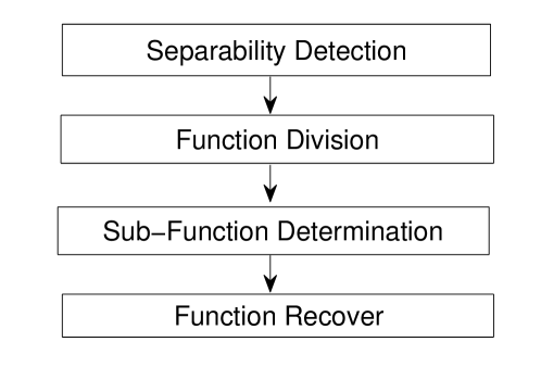
Figure 1: Work flow of divide and conquer for symbolic regression

4 Bi-correlation test

4.1 Description

The main idea of the proposed divide and conquer (D&C) method is to make use of the separability feature to simplify the search process. Therefore, the most important and fundamental step (the separability detection process in Fig. 1) is to determine whether the concerned problem is separable (at least partial separable) or not. To fulfill this task, a special technique, Bi-correlation test (BiCT), is provided in this section.

Consider independent variables $x_{1},x_{2},\cdots,x_{n}$ and the dependent $f$ as n+1 random variables, and the known data as sample points. Recall that the linear relation and correlation coefficient of two random variables has the following relations.

Lemma 1.

The two random variables $\xi$ and $\eta$ are linearly related with correlation coefficient 1 (i.e., $\rho_{\xi\eta}=1$) if and only if there exists two constants $a$, $b$ ($b\neq 0$), such that $P\{\eta=a+b\xi\}=1$.

The correlation coefficient $\rho$ could be estimated by the sample correlation coefficient $r$, which is defined as follows.

$$r=\frac{1}{n-1}\sum\limits_{i=1}^{N}\frac{(\xi_{i}-\bar{\xi})}{\sigma_{\xi}}\cdot\frac{(\eta_{i}-\bar{\eta})}{\sigma_{\eta}}$$

where $N$ is the number of observations in the sample set, $\sum$ is the summation symbol, $\xi_{i}$ is the $\xi$ value for observation i, $\bar{\xi}$ is the sample mean of $\xi$, $\eta_{i}$ is the $\eta$ value for observation i, $\bar{\eta}$ is the sample mean of $\eta$, $\sigma_{\xi}$ is the sample standard deviation of $\xi$, and $\sigma_{\eta}$ is the sample standard deviation of $\eta$.

Only continuous model functions are considered in this paper. As a result, the conclusion of Lemma 1 could be simplified as follows.

• The two random variables ${\boldsymbol{f}}_{A}$ and ${\boldsymbol{f}}_{B}$ are linearly related (${\boldsymbol{f}}_{B}=a+b{\boldsymbol{f}}_{A}$) if and only if the sample correlation coefficient $r=1$ for any given sample set.

Studies shows that the functional separability defined in the above section (See equation 6) could be observed with random sampling and linear correlation techniques.

Without the loss of generality, a simple function with three variables ($f(\boldsymbol{x})=f(x_{1},x_{2},x_{3}),x_{i}\in[a_{i},b_{i}],i=1,2,3$) is considered to illustrate the implementation of the bi-correlation test. To find out whether the first variable $x_{1}$ is separable, two correlation tests are needed.

The first correlation test is carried out as follows. A set of random sample points in $[a_{1},b_{1}]$ are generated, then these points are extended to three dimensional space with the rest variables ($x_{2}$ and $x_{3}$) fixed to a point $A$. We get a vector of function values ${\boldsymbol{f}}^{(A)}={\boldsymbol{f}}{(x_{1},A)}=(f_{1}^{A},f_{2}^{A},\cdots,f_{N}^{A})$, where $N$ is the number of sample points. Then these points are extended to three dimensional space with fixed $x_{2}$ and $x_{3}$ to another point $B$, We get another vector ${\boldsymbol{f}}^{(B)}={\boldsymbol{f}}{(x_{1},B)}=(f_{1}^{B},f_{2}^{B},\cdots,f_{N}^{B})$. It is obviously that the two vectors $f^{(A)}$ and $f^{(B)}$ will be linearly related if $x_{1}$ is separable. However, it is easy to show that this linear relation could NOT ensure its separability.

Then it comes to the second correlation test. Another set of random sample points in $[a_{2},b_{2}]\times[a_{3},b_{3}]$ are generated, then these points are extended to three dimensional space with the rest variable(s) ($x_{1}$ in this case) fixed to a point $C$, and get a vector ${\boldsymbol{f}}^{(C)}={\boldsymbol{f}}{(C,x_{2},x_{3})}$. Similarly, another vector ${\boldsymbol{f}}^{(D)}={\boldsymbol{f}}{(D,x_{2},x_{3})}$ is obtained. Again, the two vectors ${\boldsymbol{f}}^{(C)}$ and ${\boldsymbol{f}}^{(D)}$ needs to be linearly related to ensure the separability of $x_{1}$.

4.2 Proposition

Without the loss of generality, suppose we have a scalar function ${f}(\boldsymbol{x})$ with $n$ continuous variables (${f}:{\mathbb{R}^{n}}\mapsto\mathbb{R}$, $\boldsymbol{x}\in\Omega\subset{\mathbb{R}^{n}}$, and $\Omega=[a_{1},b_{1}]\times[a_{2},b_{2}]\times\cdots\times[a_{n},b_{n}]$), and need to find out whether the first $m$ variable combination $(x_{1},x_{2},\cdots,x_{m})$ are separable. Let the matrix $X_{1}$ be a set of $N$ random sample points from the subset $[a_{1},b_{1}]\times[a_{2},b_{2}]\times\cdots\times[a_{m},b_{m}]\subset\mathbb{R}^{m}$, and

$${X_{1}}=\left[{\begin{array}[]{*{20}{c}}{{x_{1}^{(1)}}}&{{x_{2}^{(1)}}}&\cdots&{{x_{m}^{(1)}}}\\ {{x_{1}^{(2)}}}&{{x_{2}^{(2)}}}&\cdots&{{x_{m}^{(2)}}}\\ \cdots&\cdots&\cdots&\cdots\\ {{x_{1}^{(N)}}}&{{x_{2}^{(N)}}}&\cdots&{{x_{m}^{(N)}}}\end{array}}\right].$$

The rest variables $x_{m+1},x_{m+2},\cdots,x_{n}$ are fixed to two given points A and B in the subset $[a_{m+1},b_{m+1}]\times[a_{m+2},b_{m+2}]\times\cdots\times[a_{n},b_{n}]\subset\mathbb{R}^{n-m}$, i.e., $\boldsymbol{x}_{A}=({{x_{m+1}}^{(A)}},{{x_{m+2}}^{(A)}},\cdots,{{x_{n}}^{(A)}})$, $\boldsymbol{x}_{B}=({{x_{m+1}}^{(B)}},{{x_{m+2}}^{(B)}},\cdots,{{x_{n}}^{(B)}})$.
Let the matrix ${X_{2}}^{(A)}=\left[\begin{gathered}1\hfill\\ 1\hfill\\ \cdots\hfill\\ 1\hfill\\ \end{gathered}\right]\boldsymbol{x}_{A}=\left[{\begin{array}[]{*{20}{c}}{{x_{m+1}}^{(A)}}&{{x_{m+2}}^{(A)}}&\cdots&{{x_{n}}^{(A)}}\\ {{x_{m+1}}^{(A)}}&{{x_{m+2}}^{(A)}}&\cdots&{{x_{n}}^{(A)}}\\ \cdots&\cdots&\cdots&\cdots\\ {{x_{m+1}}^{(A)}}&{{x_{m+2}}^{(A)}}&\cdots&{{x_{n}}^{(A)}}\end{array}}\right]$, and ${X_{2}}^{(B)}=\left[\begin{gathered}1\hfill\\ 1\hfill\\ \cdots\hfill\\ 1\hfill\\ \end{gathered}\right]\boldsymbol{x}_{B}$.
Let the extended matrix ${X_{A}}=\left[{\begin{array}[]{*{20}{c}}{{X_{1}}}&{{X_{2}}^{(A)}}\end{array}}\right]$, and ${X_{B}}=\left[{\begin{array}[]{*{20}{c}}{{X_{1}}}&{{X_{2}}^{(B)}}\end{array}}\right]$.
Let ${\boldsymbol{f}_{A}}$ be the vector of which the $i$-th element is the function value of the $i$-th row of matrix ${X_{A}}$, i.e., ${\boldsymbol{f}_{A}}=f({X_{A}})$, and ${\boldsymbol{f}_{B}}$ is similarly defined, ${\boldsymbol{f}_{B}}=f({X_{B}})$.

Lemma 2.

The two vectors ${\boldsymbol{f}_{A}}$ and ${\boldsymbol{f}_{B}}$ are linearly related if the function $f(\boldsymbol{x})$ is separable with respect to the first $m$ variable combination $(x_{1},x_{2},\cdots,x_{m})$.

Proof.

Since the first $m$ variable combination $(x_{1},x_{2},\cdots,x_{m})$ are separable, from definition 1, we have $f(\boldsymbol{x})=\varphi_{1}(x_{1},x_{2},\cdots,x_{m})\otimes\varphi_{2}(x_{m+1},x_{m+2},\cdots,x_{n})$. Accordingly, the vector ${\boldsymbol{f}_{A}}=f({X_{A}})=\varphi_{1}(X_{1})\otimes\varphi_{2}({X_{2}^{A}})=\varphi_{1}(X_{1})\otimes k_{A}$, where $\otimes$ is a component-wise binary operation, and $k_{A}=\varphi_{2}(\boldsymbol{x}_{A})$ is a scalar. Similarly, the vector ${\boldsymbol{f}_{B}}=\varphi_{1}(X_{1})\otimes k_{B}$. As a result,

$${\boldsymbol{f}}_{A}=\left\{{\begin{array}[]{*{20}{l}}{{k_{A}}/{k_{B}}\cdot{{\boldsymbol{f}}_{B}}}&{{\text{if }}\otimes{\text{ is times}}}\\ {{k_{A}}-{k_{B}}+{{\boldsymbol{f}}_{B}}}&{{\text{if }}\otimes{\text{ is plus}}}\\ {{k_{B}}-{k_{A}}+{{\boldsymbol{f}}_{B}}}&{{\text{if }}\otimes{\text{ is minus}}}\end{array}}\right.$$

which means the two vectors ${\boldsymbol{f}_{A}}$ and ${\boldsymbol{f}_{B}}$ are linearly related. ∎

On the other hand, if the first $m$ variables are fixed to two given points C and D, and the rest of $n-m$ variables are randomly sampled. A similar proposition could be concluded as follows. Let
${X_{1}}^{(C)}=\left[\begin{gathered}1\hfill\\ 1\hfill\\ \cdots\hfill\\ 1\hfill\\ \end{gathered}\right]\left[{\begin{array}[]{*{20}{c}}{{x_{1}}^{(C)}}&{{x_{2}}^{(C)}}&\cdots&{{x_{m}}^{(C)}}\end{array}}\right]=\left[{\begin{array}[]{*{20}{c}}{{x_{1}}^{(C)}}&{{x_{2}}^{(C)}}&\cdots&{{x_{m}}^{(C)}}\\ {{x_{1}}^{(C)}}&{{x_{2}}^{(C)}}&\cdots&{{x_{m}}^{(C)}}\\ \cdots&\cdots&\cdots&\cdots\\ {{x_{1}}^{(C)}}&{{x_{2}}^{(C)}}&\cdots&{{x_{m}}^{(C)}}\end{array}}\right]$,
${X_{1}}^{(D)}=\left[\begin{gathered}1\hfill\\ 1\hfill\\ \cdots\hfill\\ 1\hfill\\ \end{gathered}\right]\left[{\begin{array}[]{*{20}{c}}{{x_{1}}^{(D)}}&{{x_{2}}^{(D)}}&\cdots&{{x_{m}}^{(D)}}\end{array}}\right]$,
${X_{2}}=\left[{\begin{array}[]{*{20}{c}}{{x_{m+1}^{(1)}}}&{{x_{m+2}^{(1)}}}&\cdots&{{x_{n}^{(1)}}}\\ {{x_{m+1}^{(2)}}}&{{x_{m+2}^{(2)}}}&\cdots&{{x_{n}^{(2)}}}\\ \cdots&\cdots&\cdots&\cdots\\ {{x_{m+1}^{(N)}}}&{{x_{m+2}^{(N)}}}&\cdots&{{x_{n}^{(N)}}}\end{array}}\right],$ the $N\times n$ matrix ${X_{C}}=\left[{\begin{array}[]{*{20}{c}}{{X_{1}}^{(C)}}&{{X_{2}}}\end{array}}\right]$, and ${X_{D}}=\left[{\begin{array}[]{*{20}{c}}{{X_{1}}^{(D)}}&{{X_{2}}}\end{array}}\right]$. Let ${\boldsymbol{f}_{C}}$ be the vector of which the $i$-th element is the function value of the $i$-th row of matrix ${X_{C}}$, i.e., ${\boldsymbol{f}_{C}}=f({X_{C}})$, and ${\boldsymbol{f}_{D}}$ is similarly defined, ${\boldsymbol{f}_{D}}=f({X_{D}})$.

Lemma 3.

The two vectors ${\boldsymbol{f}_{C}}$ and ${\boldsymbol{f}_{D}}$ are linearly related if the function $f(\boldsymbol{x})$ is separable with respect to the first $m$ variable combination $(x_{1},x_{2},\cdots,x_{m})$.

Proof.

Since the first $m$ variable combination $(x_{1},x_{2},\cdots,x_{m})$ are separable, from definition 1, we have $f(\boldsymbol{x})=\varphi_{1}(x_{1},x_{2},\cdots,x_{m})\otimes\varphi_{2}(x_{m+1},x_{m+2},\cdots,x_{n})$. Accordingly, the vector ${\boldsymbol{f}_{C}}=f({X_{C}})=\varphi_{1}(X_{1}^{C})\otimes\varphi_{2}({X_{2}})=k_{C}\otimes\varphi_{2}(X_{2})$, where $\otimes$ is a component-wise binary operation, and the scalar $k_{C}=\varphi_{1}(\boldsymbol{x}_{C})$. Similarly, the vector ${\boldsymbol{f}_{D}}=k_{D}\otimes\varphi_{2}(X_{2})$. As a result,

$${\boldsymbol{f}}_{C}=\left\{{\begin{array}[]{*{20}{l}}{{k_{C}}/{k_{D}}\cdot{{\boldsymbol{f}}_{D}}}&{{\text{if }}\otimes{\text{ is times}}}\\ {{k_{C}}-{k_{D}}+{{\boldsymbol{f}}_{D}}}&{{\text{if }}\otimes{\text{ is plus or minus}}}\end{array}}\right.$$

which means the two vectors ${\boldsymbol{f}_{C}}$ and ${\boldsymbol{f}_{D}}$ are linearly related. ∎

The above lemmas show that two function-value vectors must be linearly related if the target function has the separability feature, while the separable variables (or their complement variables) are fixed. These are necessary conditions for the separability identification of target function. The sufficient and necessary conditions are given as follows.

Theorem 1.

The function $f(\boldsymbol{x})$ is separable with respect to the first $m$ variable combination $(x_{1},x_{2},\cdots,x_{m})$ if and only if both of the flowing statements are true.
(1) Any two function-value vectors with fixed $(x_{1},x_{2},\cdots,x_{m})$ are linearly related;
(2) Any two function-value vectors with fixed $(x_{m+1},x_{m+2},\cdots,x_{n})$ are linearly related.

Proof.

From Lemma 2, and Lemma 3, we can conclude that the necessary conditions of the theorem hold. The sufficient conditions can be proved by contradiction. Suppose the separable form $f\left(\boldsymbol{x}\right)={\varphi_{1}}\left({{x_{1}},{x_{2}},\cdots,{x_{m}}}\right)\otimes{\varphi_{2}}\left({{x_{m+1}},{x_{m+2}}\cdots,{x_{n}}}\right)$ can not be derived from the above two conditions. Thus, there is at least one non-separable variable presented in both sub-functions, ${\varphi_{1}}$ and ${\varphi_{2}}$. Without loss of generality, we assume ${x_{m}}$ to be this non-separable variable. That is,

$$f\left(\boldsymbol{x}\right)={\varphi_{1}}\left({{x_{1}},{x_{2}},\cdots,{x_{m}}}\right)\otimes{\varphi_{2}}\left({{x_{m}},{x_{m+1}},{x_{m+2}}\cdots,{x_{n}}}\right).$$ (7)

Similarly, the process of sampling for the first correlation test can be given as

$${X_{1}}=\left[{\begin{array}[]{*{20}{c}}{x_{1}^{\left(1\right)}}&{x_{2}^{\left(1\right)}}&\cdots&{x_{m}^{\left(1\right)}}\\ {x_{1}^{\left(2\right)}}&{x_{2}^{\left(2\right)}}&\cdots&{x_{m}^{\left(2\right)}}\\ \vdots&\vdots&{}\hfil&\vdots\\ {x_{1}^{\left(N\right)}}&{x_{2}^{\left(N\right)}}&\cdots&{x_{m}^{\left(N\right)}}\end{array}}\right],$$ (8)

$$\tilde{X}_{2}^{\left(A\right)}=\left[{\begin{array}[]{*{20}{c}}{x_{m}^{\left(1\right)}}&{x_{m+1}^{\left(A\right)}}&{x_{m+2}^{\left(A\right)}}&\cdots&{x_{n}^{\left(A\right)}}\\ {x_{m}^{\left(2\right)}}&{x_{m+1}^{\left(A\right)}}&{x_{m+2}^{\left(A\right)}}&\cdots&{x_{m}^{\left(A\right)}}\\ \vdots&\vdots&\vdots&{}\hfil&\vdots\\ {x_{m}^{\left(N\right)}}&{x_{m+1}^{\left(A\right)}}&{x_{m+2}^{\left(A\right)}}&\cdots&{x_{m}^{\left(A\right)}}\end{array}}\right],$$ (9)

and

$$\tilde{X}_{2}^{\left(B\right)}=\left[{\begin{array}[]{*{20}{c}}{x_{m}^{\left(1\right)}}&{x_{m+1}^{\left(B\right)}}&{x_{m+2}^{\left(B\right)}}&\cdots&{x_{n}^{\left(B\right)}}\\ {x_{m}^{\left(2\right)}}&{x_{m+1}^{\left(B\right)}}&{x_{m+2}^{\left(B\right)}}&\cdots&{x_{m}^{\left(B\right)}}\\ \vdots&\vdots&\vdots&{}\hfil&\vdots\\ {x_{m}^{\left(N\right)}}&{x_{m+1}^{\left(B\right)}}&{x_{m+2}^{\left(B\right)}}&\cdots&{x_{m}^{\left(B\right)}}\end{array}}\right].$$ (10)

Let the extended matrix ${X^{\prime}_{A}}=\left[{\begin{array}[]{*{20}{c}}{{X_{1}}}&{\tilde{X}_{2}^{\left(A\right)}}\end{array}}\right]$, and ${X^{\prime}_{B}}=\left[{\begin{array}[]{*{20}{c}}{{X_{1}}}&{\tilde{X}_{2}^{\left(B\right)}}\end{array}}\right]$. Thus,

$${\boldsymbol{f}^{\prime}_{A}}{\text{ = }}f\left({{{X^{\prime}}_{A}}}\right){\text{ = }}{\varphi_{1}}\left({{X_{1}}}\right)\otimes{\varphi_{2}}\left({\tilde{X}_{2}^{\left(A\right)}}\right){\text{ = }}{\varphi_{1}}\left({{X_{1}}}\right)\otimes\boldsymbol{\alpha},$$ (11)

and

$${\boldsymbol{f}^{\prime}_{B}}{\text{ = }}f\left({{{X^{\prime}}_{B}}}\right){\text{ = }}{\varphi_{1}}\left({{X_{1}}}\right)\otimes{\varphi_{2}}\left({\tilde{X}_{2}^{\left(B\right)}}\right){\text{ = }}{\varphi_{1}}\left({{X_{1}}}\right)\otimes\boldsymbol{\beta}$$ (12)

are defined, where $\boldsymbol{\alpha}$ and $\boldsymbol{\beta}$ are function-value vectors of ${\varphi_{2}}\left({\tilde{X}_{2}^{\left(A\right)}}\right)$ and ${\varphi_{2}}\left({\tilde{X}_{2}^{\left(B\right)}}\right)$ respectively. As a result,

$${\boldsymbol{f}^{\prime}_{A}}{\text{ = }}\left\{{\begin{array}[]{*{20}{l}}\boldsymbol{\gamma}\cdot{{\boldsymbol{f}^{\prime}}_{B}}&{\text{ if }\otimes\text{ is times}}\\ \boldsymbol{\alpha}-\boldsymbol{\beta}+{{\boldsymbol{f}^{\prime}}_{B}}&{\text{ if }\otimes\text{ is plus}}\\ \boldsymbol{\beta}-\boldsymbol{\alpha}+{{\boldsymbol{f}^{\prime}}_{B}}&{\text{ if }\otimes\text{ is minus}}\\ \end{array}}\right.$$ (13)

where $\boldsymbol{\gamma}=\left({{{{\alpha_{1}}}\mathord{\left/{\vphantom{{{\alpha_{1}}}{{\beta_{1}}}}}\right.\kern-1.2pt}{{\beta_{1}}}},{{{\alpha_{2}}}\mathord{\left/{\vphantom{{{\alpha_{2}}}{{\beta_{2}}}}}\right.\kern-1.2pt}{{\beta_{2}}}},\cdots,{{{\alpha_{N}}}\mathord{\left/{\vphantom{{{\alpha_{N}}}{{\beta_{N}}}}}\right.\kern-1.2pt}{{\beta_{N}}}}}\right)$. From the lemmas, we know that, two vectors $\boldsymbol{f}^{\prime}_{A}$ and ${\boldsymbol{f}^{\prime}}_{B}$ are linearly related if they are in the relation of $\boldsymbol{f}^{\prime}_{A}=k_{1}\cdot{\boldsymbol{f}^{\prime}}_{B}+k_{2}$, where $k_{1}$ and $k_{2}$ are constant scalars, $k_{1}\neq 0$. But, from the above discussion, the components of all the three vectors, $\boldsymbol{\gamma}$, $\boldsymbol{\alpha}-\boldsymbol{\beta}$ and $\boldsymbol{\beta}-\boldsymbol{\alpha}$, are not constant, due to the randomness of sample points $\left({x_{m}^{\left(1\right)},x_{m}^{\left(2\right)},\;\cdots,x_{m}^{\left(N\right)}}\right)$. This contradicts the supposition that the two vectors $\boldsymbol{f}^{\prime}_{A}$ and ${\boldsymbol{f}^{\prime}}_{B}$ are linearly related, and so Equation (7) cannot hold. ∎

4.3 Notes on BiCT

The proposed technique is called bi-correlation test (BiCT) since two complementary correlation tests are simultaneously carried out to determine whether a variable or a variable-combination is separable.

The above process is illustrated with two sub-functions, and it could be extended to determine the separability of a function with more sub-functions. However, if the binary operators $\otimes_{1},\otimes_{2},\cdots,\otimes_{m}$ in equation (6) are mutually different with mixed times and plus or minus, the extension might be a little difficult. This issue will be left for the future work. Hereafter, we assume that the binary operators in equation (6) are the same, i.e, $\otimes_{i}$= times or $\otimes_{i}$= plus or minus for all $i=1,2,\cdots,m$, for simplicity. In this case, the extension process is very easy and omitted here.

To enhance the stability and efficiency of the algorithm, the distribution of sample points should be as uniform as possible. Therefore, controlled sampling methods such as Latin hypercube sampling (Beachkofski and Grandhi, 2002) and orthogonal sampling (Steinberg and Lin, 2006) are preferred for sample generation.

For the correlation test, any of correlation methods could be used. That is, Pearson’s r method, Spearman’s rank order correlation, and Kendall’s $\tau$ correlation are all effective for BiCT.

Take the function $f(\boldsymbol{x})=0.8+0.6*(x_{1}^{2}+\cos(x_{1}))*\sin(x_{2}+x_{3})*(x_{2}-x_{3}),x\in[-3,3]^{3}$, as an example, the first sample set consists of 13 uniformly distributed points in $[-3,3]$, and the second sample set consists of 169 uniformly distributed points in $[-3,3]^{2}$. The correlation tests could be illustrated as in Fig. 2. As can be seen that the function-value vectors $\boldsymbol{f}^{A}$ and $\boldsymbol{f}^{B}$ are linearly related (Fig. 2(b)), in which the variable $x_{2}$ and $x_{3}$ are fixed when considering the first variable $x_{1}$ (Fig. 2(a)). Similarly, to find out the separability of variable combination ($x_{2},x_{3}$), the first variable $x_{1}$ is fixed (Fig. 2(c)). The corresponding function-value vectors $\boldsymbol{f}^{C}$ and $\boldsymbol{f}^{D}$ are linearly related (Fig. 2(d))

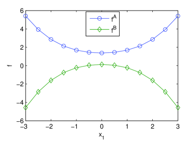
(a) ($x_{2},x_{3}$) are fixed

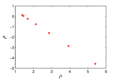
(b) $\boldsymbol{f}^{A}\leftrightarrow\boldsymbol{f}^{B}$

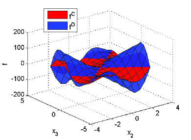
(c) $x_{1}$ are fixed

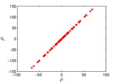
(d) $\boldsymbol{f}^{C}\leftrightarrow\boldsymbol{f}^{D}$

Figure 2: Demo of separability detection process of BiCT

The D&C method with BiCT technique is described with functions of explicit expressions. While in practical applications, no explicit expression is available. In this case, some modifications need to adapt for D&C method. In fact, for data-driven modeling problems, a surrogate model of black-box type could be established as the underlying target function (Forrester et al., 2008) in advance. Then the rest steps are the same as above discussions.

5 Numerical results

5.1 Analysis on Computing time

The computing time ($t$) of a genetic programming with the proposed divide and conquer (D&C) method consists three parts:

$$t=t_{1}+t_{2}+t_{3}$$ (14)

where $t_{1}$ is for the separability detection, $t_{2}$ for sub-function determination, and $t_{3}$ for function recover. Note that both the separability detection and function recover processes are double-precision operations and thus cost much less time than the sub-function determination process. That is, $t\approx t_{2}$.

It is obviously that the CPU time for determining all sub-functions ($t_{2}$) is much less than that of determining the target function directly ($t_{d}$). Next, a typical genetic programming, parse matrix evolution (PME), is taken as the optimization driver (other GP algorithms should also work) to show the performance of D&C.

Table 1: A mapping table for parse-matrix evolution

$a_{\cdot 1}$	-5	-4	-3	-2	-1	0	1	2	3	4	5
T	$\sqrt{\cdot}$	ln	cos	/	-	skip	+	*	sin	exp	$(\cdot)^{2}$
$a_{\cdot 2},a_{\cdot 3}$	-5	-4	-3	-2	-1	0	1	2	$\cdots$	d
expr	$\lambda_{2}$	$\lambda_{1}$	$f$	$f_{2}$	$f_{1}$	1.0	$x_{1}$	$x_{2}$	$\cdots$	$x_{d}$
$a_{\cdot 4}$	-1	0	1
$f\rightarrow f_{k}$	skip	$f_{1}$	$f_{2}$

Suppose that the dimension of the target function is $d$, the height of the parse-matrix $h$, and the mapping Table as in Table 1, then the parse-matrix entries $a_{\cdot 1}\in{-5,-4,...,4,5}$, $a_{\cdot j}\in{-5,-4,\cdots,d}$, ($j=1,2$), and $a_{\cdot 4}\in{-1,0,1}$. Thus the parse-matrix $(a_{ij})_{h\times 4}$ have as many as $(11*(6+d)*(6+d)*3)^{h}$ possible combinations. Thus the CPU time of determining the target function directly satisfies

$$t_{d}\sim(11*(6+d)*(6+d)*3)^{h}.$$ (15)

This means that the searching time of determining a target function will increase exponentially with model complexity. Using D&C, only the sub-functions are needed to determinate, and each sub-function has less dimension $d$ and less complexity $h$. Therefore, it will cost much less CPU time. In fact, by D&C powered GP, the CPU time will increase only linearly with dimensions, provided that the target function is completely separable.

Take equation (2) in Section 1 as an example. Without D&C, to search directly, the control parameters of PME should be set as follows: $d=5$, $h\geq 9$. From equation (15), the order of required CPU time $t_{d}=O(2.58\cdot 10^{32})$.

Using D&C powered PME, the required CPU time will be much less. In fact, after the separation detection, the function is divided into for sub-functions as follows.

$${q_{s}}=1.83\times{10^{-4}}\boxed{{v^{3}}}\cdot\boxed{\sqrt{\rho}}\cdot\boxed{1/\sqrt{R}}\cdot\boxed{(1-{h_{w}}/{h_{s}})}$$

For the sub-function $v^{3}$, $1/\sqrt{R}$, and $1-h_{w}/h_{s}$, the control parameters of PME should be set as $d=1$, $h\geq 2$. For the sub-function $\sqrt{\rho}$, $d=1$, $h\geq 1$. As a result, $t_{2}\approx 4*O(2.61\cdot 10^{6})=O(10^{7})$ by equation (15), which means the D&C method could reduce the computational effort by orders of magnitude.

5.2 Program timing

Next, two illustrative examples are presented to show how much time the D&C technique could save in practical applications.

Again, equation (1) and equation (2) are set as the target function, respectively. For equation (1), the sample set consists 100 observations uniformly distributed in [1,10] degree and [1000, 10000] (i.e., $\theta$=1:10; $Re_{x}$ = 1000:1000:10000). The angle $\theta$ is fixed to 5 degree while detecting the sub-function $f_{1}(Re_{x})$, and the Renold number $Re_{x}$ is fixed to 5000 while detecting the sub-function $f_{2}(\theta)$.

For equation (2), the sample set consists 30000 observations uniformly distributed in a box in $R^{5}$ (i.e., $v=500:100:1000;\rho=0.0001:0.0001:0.001;R=0.01:0.01:0.1;h_{w}=10000:10000:50000;h_{s}=100000:100000:1000000$). The velocity of free-stream $v$, density of air $\rho$, radius of nose $R$, Wall enthalpy $h_{w}$, and total enthalpy $h_{s}$ are fixed to 800 $m/s^{2}$, 0.0005 kg/$m^{3}$, 0.05 m, 20000 J/kg, and 200000 J/kg, respectively, while detecting the sub-functions.

In both tests, the program stops when the current model is believed good enough: $1-R^{2}<1.0\cdot 10^{-10}$, where $R^{2}=1-\frac{SSE}{SST}$ can be regarded as the fraction of the total sum of squares that has ‘explained by’ the model. To suppress the affect of randomness of PME, 10 runs are carried out for each target function, and the averaged CPU time on a PC using a single CPU core (Intel(R) Core (TM) i7-4790 CPU @3.60GHz) is recorded to show its performance. The test results (see Table 2, and Table 3) show that D&C technique can save CPU time remarkably. For equation (1), PME needs about 12 minutes and 26 seconds to get an alternative of the target function without D&C technique, while the D&C powered PME needs only about 11.2 seconds, which is much faster than the original algorithm. Similar conclusion could also seen from the test results of equation (2) (see Table 3). Note that the total time of D&C powered PME includes $t_{1}$, $t_{2}$ and $t_{3}$ (See Equ. 14), and $t_{1}+t_{3}\approx 0.2$ for Equ. (1), 0.3 for Equ. (2).

Table 2: Performance of PME on detecting Equ. (1) (with and without D&C)

Target Function	CPU time	Result Expression
For D&C powered PME
$f_{1}(Re_{x})$	3s	$St=0.1978/\sqrt{Re_{x}}$
$f_{2}(\theta)$	8s∗	$St=0.03215*\theta-0.01319*\theta^{3}$
Total time	11.2s
PME without D&C
$f(Re_{x},\theta)$	12m26s∗	$St=2.274*\theta*\cos(0.9116*\theta)/\sqrt{Re_{x}}$
Total time	746s

^∗ PME failed to get the exact result, but always result in an alternative function with fitting error of zero in double precision (i.e., $1-R^{2}=0.0$).

Table 3: Performance of PME on detecting target Equ. (2)(with and without D&C)

Target Function	CPU time	Result Expression
For D&C powered PME
$f_{1}(v)$	3s	$q_{s}=1.647\cdot 10^{-5}*v^{3}$
$f_{2}(\rho)$	2s	$q_{s}=3.77\cdot 10^{5}*\sqrt{\rho}$
$f_{3}(R)$	4s	$q_{s}=6.49\cdot 10^{3}*\sqrt{0.08442/R}$
$f_{4}(h_{w},h_{s})$	9s	$q_{s}=9370-9370*h_{w}/h_{s}$
Total time	18.3s
PME without D&C
$f(v,\rho,R,hw,hs)$	85m43s	$q_{s}=0.000183*v^{3}*\sqrt{\rho/R}*(1-h_{w}/h_{s})$
Total time	5143s

6 Conclusion

The divide and conquer (D&C) method for symbolic regression has been presented. The main idea is to make use of the separability feature of the underling target function to simplify the search process. In D&C, the target function is divided into a number of sub-functions based on the information of separability detection, and the sub-functions are then determined by any of a genetic programming (GP) algorithms.

The most important and fundamental step in D&C is to identify the separability feather of the concerned system. To fulfill this task, a special algorithm, bi-correlation test (BiCT), is also provided for separability detection in this paper.

The study shows that D&C can accelerate the convergence speed of GP by orders of magnitude without losing the generality, provided that the target function has the feature of separability, which is usually the case in practical engineering applications.

References

References

- Anderson (2006) Anderson, J., 2006. Hypersonic and High-Temperature Gas Dynamics (2nd ed.). American Institute of Aeronautics and Astronautics, Inc., Virginia.
-
Beachkofski and Grandhi (2002)
Beachkofski, B., Grandhi, R., APRL 2002. Improved distributed hypercube
sampling. In: 43rd AIAA/ASME/ASCE/AHS/ASC Structures, Structural Dynamics,
and Materials Conference, Structures, Structural Dynamics, and Materials and
Co-located Conferences. AIAA paper no. 2002-1274. Denver, Colorado.
URL https://doi.org/10.2514/6.2002-1274 - Berenguel et al. (2013) Berenguel, L., Casado, L. G., García, I., Hendrix, E. M. T., Messine, F., 2013. On interval branch-and-bound for additively separable functions with common variables. Journal of Global Optimization 56 (3), 1101–1121.
-
Chen et al. (2017)
Chen, C., Luo, C., Jiang, Z., 2017. Elite bases regression: A real-time
algorithm for symbolic regression.
URL https://arxiv.org/abs/1704.07313 - d’Avezac et al. (2011) d’Avezac, M., Botts, R., Mohlenkamp, M. J., Zunger, A., 2011. Learning to predict physical properties using sums of separable functions. SIAM Journal on Scientific Computing 33 (6), 3381–3401.
- Forrester et al. (2008) Forrester, A., Sobester, A., Keane, A., 2008. Engineering design via surrogate modelling: a practical guide. John Wiley & Sons, Hoboken, New Jersey.
- Koza (2008) Koza, J. R., 2008. Genetic programming: on the programming of computers by means of natural selection. MIT Press, Cambridge, MA.
- Luo and Zhang (2012) Luo, C., Zhang, S.-L., 2012. Parse-matrix evolution for symbolic regression. Engineering Applications of Artificial Intelligence 25 (6), 1182–1193.
- McConaghy (2011) McConaghy, T., 2011. FFX: Fast, Scalable, Deterministic Symbolic Regression Technology. Springer New York, New York, NY, pp. 235–260.
-
O’Neill and Ryan (2001)
O’Neill, M., Ryan, C., Aug. 2001. Grammatical evolution. IEEE Trans. Evol. Comp
5 (4), 349–358.
URL http://dx.doi.org/10.1109/4235.942529 - Schmidt and Lipson (2009) Schmidt, M., Lipson, H., 2009. Distilling free-form natural laws from experimental data. Science 324 (59236), 81–85.
- Steinberg and Lin (2006) Steinberg, D. M., Lin, D. K. J., 2006. A construction method for orthogonal latin hypercube designs. Biometrika 93 (2), 279–288.