Permutation Tests for Infection Graphs

Justin Khim Machine Learning Department, Carnegie Mellon University, Pittsburgh, PA 15213.    Po-Ling Loh Department of Statistics, University of Wisconsin, Madison, WI 53706 and Department of Statistics, Columbia University, New York, NY 10027.
(December 16, 2019)
Abstract

We formulate and analyze a novel hypothesis testing problem for inferring the edge structure of an infection graph. In our model, a disease spreads over a network via contagion or random infection, where the times between successive contagion events are independent exponential random variables with unknown rate parameters. A subset of nodes is also censored uniformly at random. Given the observed infection statuses of nodes in the network, the goal is to determine the underlying graph. We present a procedure based on permutation testing, and we derive sufficient conditions for the validity of our test in terms of automorphism groups of the graphs corresponding to the null and alternative hypotheses. Our test is easy to compute and does not involve estimating unknown parameters governing the process. We also derive risk bounds for our permutation test in a variety of settings, and relate our test statistic to approximate likelihood ratio testing and maximin tests. For graphs not satisfying the necessary symmetries, we provide an additional method for testing the significance of the graph structure, albeit at a higher computational cost. We conclude with an application to real data from an HIV infection network.

1 Introduction

Information, diseases, and the adoption of certain behaviors may spread according to a network of relationships connecting susceptible individuals [2, 12, 28, 40, 43]. Natural questions to address include (a) predicting the pathway or scope of a disease; (b) inferring the source; and (c) identifying optimal interventions to slow the spread of the epidemic. The answers to these questions may vary depending on the stochastic mechanism governing the spread of disease between individuals, and/or the rate of recovery.

Algorithms for addressing such questions often assume knowledge of the underlying graph structure [6, 8, 9]. For instance, in the influence maximization problem, the goal is to identify an optimal set of nodes to initially infect in order to propagate a certain behavior as widely as possible [16, 31]. Due to submodularity of the influence function, one may obtain a constant factor approximation to the influence-maximizing subset using a simple greedy algorithm. However, both the connectivity of the network and edge transmission parameters must be known in order to successfully execute the algorithm [11]. Similarly, algorithms for network immunization, which aim to eliminate an epidemic by performing targeted interventions, assume knowledge of the graph [1, 13, 44]. In real-world applications, however, prior knowledge of the edge structure of the underlying network or parameters of the infection spreading mechanism may be unavailable.

Accordingly, the focus of our paper is the inference problem of identifying the underlying network based on observed infection data. One approach involves employing tools from graphical model estimation, since the graphical model corresponding to joint vectors of infection times coincides with the unknown network [24, 42]. However, these methods critically leverage the availability of time-stamped data and observations of multiple (i.i.d.) infection processes spreading over the same graph. Another line of work concerns reconstructing an infection graph based on the order in which nodes are infected over multiple infection processes, and provides bounds on the number of distinct observations required to recover the edge structure of the graph. These methods are attractive in that they do not assume a particular stochastic spreading model, and are even guaranteed to reconstruct the true network when the observations are chosen adversarially [3, 27]. On the other hand, data from multiple infections are still assumed to be available.

In contrast to these papers, we are interested in studying scenarios where infection data are available for a single snapshot of a single epidemic outbreak. For instance, if the goal is to perform optimal interventions on a network of individuals during an outbreak such as Ebola [17], data may only be available about the infection status of individuals at a given point in time. Although historic data may have been collected concerning the spread of other epidemics on the same network, there is no guarantee that the other diseases will spread according to the same mechanisms, and the network may have changed over time. Instead of employing the aforementioned graph estimation procedures based on observation vectors, we cast the problem in the form of a hypothesis test: Given two candidate graphs, our goal is to identify the graph on which the infection has propagated. This type of problem was previously studied by [39], who proposed inference procedures for testing an empty graph versus graphs satisfying “speed and spread” conditions, and for testing two graphs against each other. However, we substantially generalize their approach, removing a restrictive “independent neighborhoods” assumption and allowing for exogenous sources of infection that are not captured by edgewise contagion [41]. A graph testing problem of a somewhat similar flavor may also be found in [10], but their goal is to identify the model of network formation for a random graph, rather than determine the network underlying an epidemic outbreak.

The crux of our approach lies in permutation testing, a notion which dates back to [19]. Permutation tests are classically applied when random variables are exchangeable under the null hypothesis. The test statistic is then computed with respect to random permutations of the observation vector, and the observed statistic is compared to quantiles of the simulated distribution [25]. We adapt this technique in a novel manner to the graph testing problem. The procedure is the same as in classical permutation testing, where we recompute a certain statistic on a set of randomly chosen permutations of the infection “vector” recording the observed statuses of the nodes in the graph. Based on quantiles of the empirical histogram, we calculate a rejection rule for the test.

The key idea is that if the null hypothesis corresponds to an empty or complete graph and edge transmission rates are homogeneous, the components of the infection vector are certainly exchangeable. This is an important setting in its own right, since it allows us to determine whether a network structure describes an infection better than random contagion. As derived in our paper, however, the permutation test succeeds more generally under appropriate assumptions incorporating symmetries of both the null graph and alternative graph. We develop a sufficient condition in terms of automorphism groups of the two graphs, which are the subsets of node permutations that map edges to edges in the corresponding graphs.

A scientific motivation for graph hypothesis testing is a case when a practitioner wants to decide whether a disease is spreading according to a fixed hypothesized graph structure (or a particular graph topology) versus completely random transmissions, which would correspond to an empty graph. Another plausible scenario is when a scientist wants to test a long-standing hypothesis that a genetic network follows a particular connectivity pattern, versus a proposed alternative involving the addition or removal of certain edges. In a third setting, one might encounter two distinct graphs representing connections between individuals on different social network platforms, and hypothesize that information diffusion is governed by one graph instead of the other.

Our work significantly broadens the scope of existing approaches, as follows: (i) we model information spreads more realistically by introducing random spreading external to the network; (ii) we drop the restrictive “independent neighborhoods” assumption, which masks any knowledge of the identity of specific individuals in the hypothesized graphs; and (iii) we provide novel algorithms for the graph testing problem in these settings. Our permutation test is attractive in that it is easy to compute and bypasses the need to estimate any model parameters involved in the spreading process. This also leads to a relatively simple analysis of risk bounds for concrete graph topologies, as developed in our examples. Notably, the numerical results illustrate settings in which our algorithms succeed, whereas previously existing tests do not lead to meaningful conclusions.

For general graphs, i.e., cases where these symmetries do not exist, we provide a computationally-intensive method for hypothesis testing based on a sufficiently fine discretization of the null hypothesis space using a simple data-processing inequality argument. Importantly, we can test slight differences in edge structure between graphs, which is not possible via permutation tests. This also allows us to a build confidence set for the underlying graph structure, but it is computationally feasible only for small graphs.

The remainder of the paper is organized as follows: In Section 2, we describe the infection spreading model and invariant statistics considered in our theory. In Section 3, we outline our graph testing procedure and state the corresponding theoretical guarantees. Section 4 discusses some illustrative special cases and provides explicit risk bounds. In Section 5, we analyze our test statistics more closely in relation to likelihood ratio tests and Hunt-Stein theory for maximin tests. In Section 6, we discuss our method for testing graphs based on discretization. Section 7 describes an application of our methods to an HIV infection graph. Section 8 concludes our discussion. Additional theory, simulations, and proofs are provided in the Appendices.

2 Problem setup

We begin by establishing the notation we will use for infections and graph-based hypothesis testing. We then describe two random infection models for which our main results are applicable, followed by terminology relevant to our invariant test statistics.

2.1 Infection notation

Let 𝒢0=(𝒱,0)subscript𝒢0𝒱subscript0\mathcal{G}_{0}=(\mathcal{V},\mathcal{E}_{0}) and 𝒢1=(𝒱,1)subscript𝒢1𝒱subscript1\mathcal{G}_{1}=(\mathcal{V},\mathcal{E}_{1}) denote two undirected graphs defined over a common set of vertices 𝒱={1,,n}.𝒱1𝑛\mathcal{V}=\{1,\ldots,n\}. A random vector of infection statuses :={v}v𝒱assignsubscriptsubscript𝑣𝑣𝒱\mathcal{I}:=\{\mathcal{I}_{v}\}_{v\in\mathcal{V}} consists of entries

v={1,if v is infected,0,if v is uninfected,,if v is censored.subscript𝑣cases1if v is infected,0if v is uninfected,if v is censored.\mathcal{I}_{v}=\begin{cases}1,&\text{if $v$ is infected,}\\ 0,&\text{if $v$ is uninfected,}\\ \star,&\text{if $v$ is censored.}\end{cases}

Let 1superscript1\mathcal{I}^{1} denote the set of infected vertices, and let 0superscript0\mathcal{I}^{0} and superscript\mathcal{I}^{\star} be defined analogously. We then define the space of possible infection status vectors involving exactly k𝑘k infected vertices, c𝑐c censored vertices, and nkc𝑛𝑘𝑐n-k-c uninfected vertices, as follows:

𝕀k,c={{0,1,}n:|1|=k,||=c}.subscript𝕀𝑘𝑐conditional-setsuperscript01𝑛formulae-sequencesuperscript1𝑘superscript𝑐\mathbb{I}_{k,c}=\left\{\mathcal{I}\in\{0,1,\star\}^{n}:|\mathcal{I}^{1}|=k,\;|\mathcal{I}^{\star}|=c\right\}.

2.2 Infection models

Next, we introduce two stochastic models for generating random infection vectors on a graph 𝒢𝒢\mathcal{G}. The first model is motivated by the infection literature and borrows elements from first-passage percolation. The second is a conditional Ising model. Although the Ising model is not designed for modeling disease propagation, the two models behave similarly for small values of the spreading parameter β𝛽\beta. After describing the method for generating infection vectors in both models, we explain the random censoring mechanism. We then briefly discuss the parameter spaces involved in our hypothesis test.

2.2.1 Stochastic spreading model

Our main infection model includes the following components: spreading by contagion along edges of the network, and spreading via factors external to the network. The rates of spreading are governed by nonnegative parameters λ,β+𝜆𝛽subscript\lambda,\beta\in\mathbb{R}_{+}. We assume that an infection spreads on 𝒢𝒢\mathcal{G}, beginning at time 0, as follows:

  • (i)

    For each vertex v𝑣v, generate an independent random variable TvExp(λ)similar-tosubscript𝑇𝑣Exp𝜆T_{v}\sim\text{Exp}(\lambda).

  • (ii)

    For each edge (u,v)𝑢𝑣(u,v)\in\mathcal{E}, generate an independent random variable TuvExp(β)similar-tosubscript𝑇𝑢𝑣Exp𝛽T_{uv}\sim\text{Exp}(\beta).

  • (iii)

    For each vertex v𝑣v, define the infection time tv:=minuN(v){tu+Tuv}Tvassignsubscript𝑡𝑣subscript𝑢𝑁𝑣subscript𝑡𝑢subscript𝑇𝑢𝑣subscript𝑇𝑣t_{v}:=\min_{u\in N(v)}\{t_{u}+T_{uv}\}\wedge T_{v}, where N(v)𝑁𝑣N(v) is the set of neighbors of v𝑣v.

In other words, each vertex contracts the disease via random infection according to an exponential random variable with rate λ𝜆\lambda, and contracts the disease from an infected neighbor at rate β𝛽\beta; in particular, when 𝒢𝒢\mathcal{G} is an empty graph, each successively infected node is chosen uniformly at random. The presence of the parameter λ𝜆\lambda has the interpretation that some factors involved in spreading the disease may not be fully accounted for in the hypothesized graphs. We define tksubscript𝑡𝑘t_{k} to be the time at which the kthsuperscript𝑘thk^{\text{th}} reporting node becomes infected, and we suppose we observe the state of the graph at some time t𝑡t such that tkttk+1subscript𝑡𝑘𝑡subscript𝑡𝑘1t_{k}\leq t\leq t_{k+1}. Note that this differs slightly from the setting of the papers [32, 39, 46], where the time t𝑡t at which the node infection statuses are observed is assumed to be a known constant.

In our analysis, we frequently use the notion of paths. A path P=(P1,,Pk)𝑃subscript𝑃1subscript𝑃𝑘P=(P_{1},\ldots,P_{k}) is an ordered set of vertices, where vertex Pisubscript𝑃𝑖P_{i} is the ithsuperscript𝑖thi^{\text{th}} vertex to be infected. A given infection J𝐽J in 𝕀k,0subscript𝕀𝑘0\mathbb{I}_{k,0} corresponds to k!𝑘k! possible paths, which we collect into a set 𝔓(J)𝔓𝐽\mathfrak{P}(J). We also refer to the path random vector as 𝒫𝒫\mathcal{P}. Thus, we have the relation

(=J)=P𝔓(J)(𝒫=P),𝐽subscript𝑃𝔓𝐽𝒫𝑃\mathbb{P}(\mathcal{I}=J)=\sum_{P\in\mathfrak{P}(J)}\mathbb{P}(\mathcal{P}=P),

which we will use repeatedly in our derivations.

Finally, note that without loss of generality, we can set λ=1𝜆1\lambda=1 by rescaling β𝛽\beta: Suppose k𝑘k vertices have been infected in running the process until time t𝑡t, and we want to determine the (k+1)thsuperscript𝑘1th(k+1)^{\text{th}} infected vertex. Since all of the Tvsubscript𝑇𝑣T_{v}’s and Tuvsubscript𝑇𝑢𝑣T_{uv}’s are independent exponential random variables, the probability that an uninfected vertex v𝑣v is infected next is

(v is infected next)=λ+βNt,vλ(nk)+βNt=1+(β/λ)Nt,v(nk)+(β/λ)Nt,𝑣 is infected next𝜆𝛽subscript𝑁𝑡𝑣𝜆𝑛𝑘𝛽subscript𝑁𝑡1𝛽𝜆subscript𝑁𝑡𝑣𝑛𝑘𝛽𝜆subscript𝑁𝑡\mathbb{P}\left(v\text{ is infected next}\right)=\frac{\lambda+\beta N_{t,v}}{\lambda(n-k)+\beta N_{t}}=\frac{1+(\beta/\lambda)N_{t,v}}{(n-k)+(\beta/\lambda)N_{t}},

where Ntsubscript𝑁𝑡N_{t} is the number of edges with one infected vertex at time t𝑡t, and Nt,vsubscript𝑁𝑡𝑣N_{t,v} is the number of infected neighbors of v𝑣v. This is equivalent to the parametrization (λ,β)=(1,β/λ)superscript𝜆superscript𝛽1𝛽𝜆(\lambda^{\prime},\beta^{\prime})=(1,\beta/\lambda).

2.2.2 Conditional Ising model

We now describe the second random infection model we will consider, which can also be parametrized by β+𝛽superscript\beta\in\mathbb{R}^{+}. Let the energy of an infection J𝐽J in 𝕀k,0subscript𝕀𝑘0\mathbb{I}_{k,0} be defined by

(J):=(u,v)JuJv.assign𝐽subscript𝑢𝑣subscript𝐽𝑢subscript𝐽𝑣\mathcal{H}(J):=-\sum_{(u,v)\in\mathcal{E}}J_{u}J_{v}.

We define the uncensored conditional 01-Ising model as

Isingu(=J):=exp(β(J))J𝕀k,0exp(β(J))=1ZIsing(β)exp(βH(J)).assignsuperscriptsubscriptIsing𝑢𝐽𝛽𝐽subscriptsuperscript𝐽subscript𝕀𝑘0𝛽superscript𝐽1subscript𝑍Ising𝛽𝛽𝐻𝐽\displaystyle\mathbb{P}_{\text{Ising}}^{u}\left(\mathcal{I}=J\right):=\frac{\exp(-\beta\mathcal{H}(J))}{\sum_{J^{\prime}\in\mathbb{I}_{k,0}}\exp(-\beta\mathcal{H}(J^{\prime}))}=\frac{1}{Z_{\text{Ising}}(\beta)}\exp(-\beta H(J)). (1)

Note that we use the term “conditional” because k𝑘k of the vertices are known to be in state 111. Furthermore, we use “010101” to denote the fact that the states are 00 and 111. We use the superscript u𝑢u to emphasize the fact that the infection is uncensored.

As we shall see, infections generated by the conditional 010101-Ising model share properties with the stochastic spreading model. However, note that unlike the stochastic spreading model, the conditional Ising model does not correspond to a simple procedure for generating successive infection events as a disease propagates over 𝒢𝒢\mathcal{G}. We discuss this model because it helps highlight the properties of the random infection distribution that allow our permutation test to succeed.

2.2.3 Censoring

We assume that censored nodes are selected uniformly at random among the nodes in the graph. Our hypothesis tests are designed to be valid, conditional on the fact that c𝑐c nodes are censored. In this subsection, we define some additional notation to express the probabilities of observing particular infection vectors, conditioned on the fact that c𝑐c nodes are censored.

Given an infection vector J𝐽J that may contain censored components, we define the set 𝒰(J)𝒰𝐽\mathcal{U}(J) to consist of all infection vectors Jsuperscript𝐽J^{\prime} such that Jsuperscript𝐽J^{\prime} has no censored vertices and Jv=Jvsubscript𝐽𝑣subscriptsuperscript𝐽𝑣J_{v}=J^{\prime}_{v} for each uncensored vertex v𝑣v. Thus, Jsuperscript𝐽J^{\prime} can have between k𝑘k and k+c𝑘𝑐k+c infected vertices. We then define the measure

μ(J;β)=J𝒰(J)1(nc)u(=J),𝜇𝐽𝛽subscriptsuperscript𝐽𝒰𝐽1binomial𝑛𝑐superscript𝑢superscript𝐽\mu(J;\beta)=\sum_{J^{\prime}\in\mathcal{U}(J)}\frac{1}{\binom{n}{c}}\mathbb{P}^{u}\left(\mathcal{I}=J^{\prime}\right), (2)

where u(=J)superscript𝑢superscript𝐽\mathbb{P}^{u}(\mathcal{I}=J^{\prime}) denotes the probability of an uncensored infection from either of the two models described above. In other words, μ𝜇\mu simply computes the probability of observing a vector J𝐽J after randomly censoring c𝑐c nodes. If we define the normalizing constant

Z(β):=J𝕀k,cμ(J;β)=J𝕀k,cJ𝒰(J)1(nc)u(=J),assign𝑍𝛽subscript𝐽subscript𝕀𝑘𝑐𝜇𝐽𝛽subscript𝐽subscript𝕀𝑘𝑐subscriptsuperscript𝐽𝒰𝐽1binomial𝑛𝑐superscript𝑢superscript𝐽Z(\beta):=\sum_{J\in\mathbb{I}_{k,c}}\mu(J;\beta)=\sum_{J\in\mathbb{I}_{k,c}}\sum_{J^{\prime}\in\mathcal{U}(J)}\frac{1}{\binom{n}{c}}\mathbb{P}^{u}(\mathcal{I}=J^{\prime}), (3)

which provides the probability of observing any vector with k𝑘k infected and c𝑐c censored nodes, we see that

(=J)=1Z(β)μ(J;β)𝐽1𝑍𝛽𝜇𝐽𝛽\mathbb{P}\left(\mathcal{I}=J\right)=\frac{1}{Z(\beta)}\mu(J;\beta) (4)

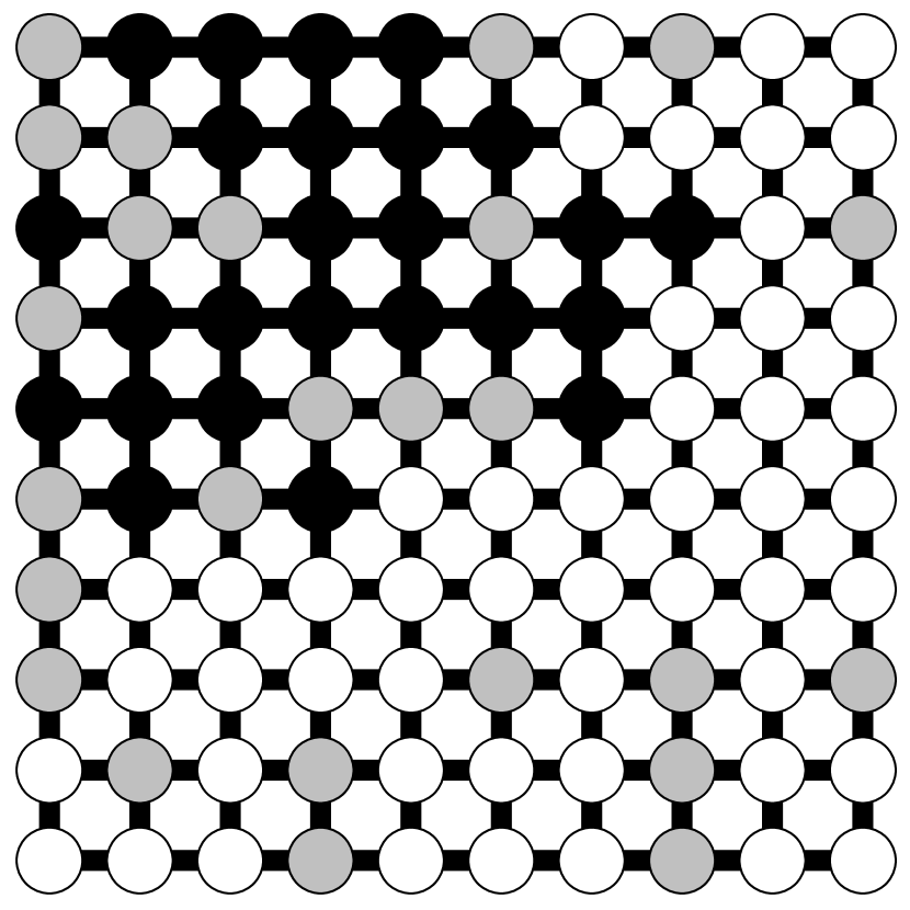
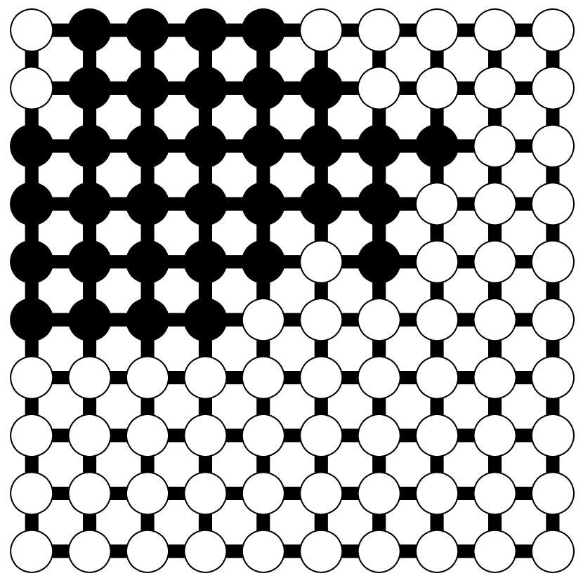
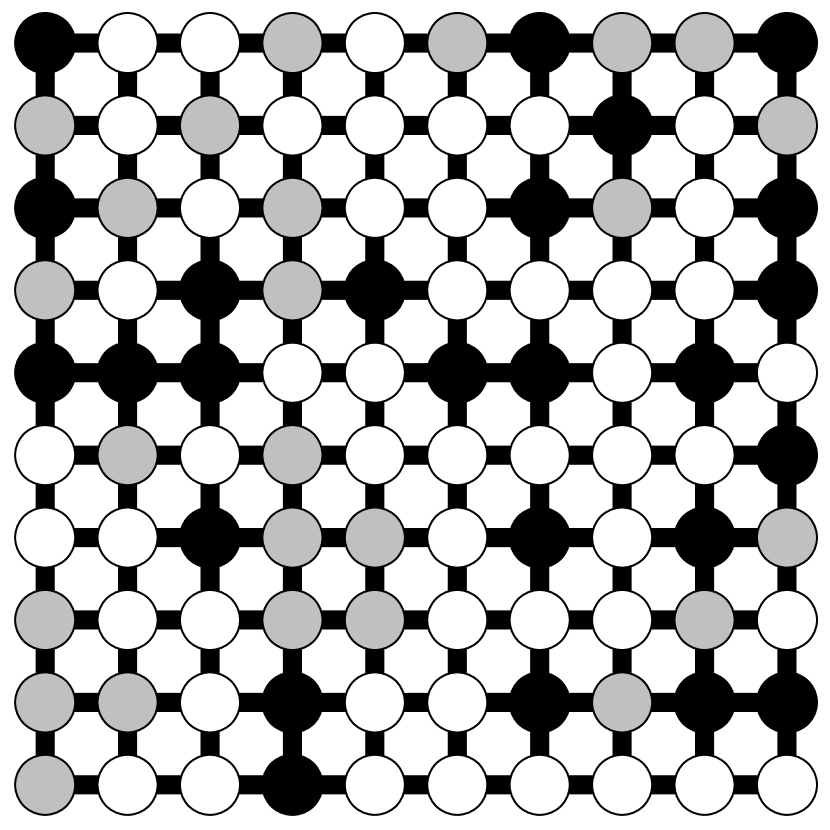
is the probability of observing infection vector J𝐽J, conditioned on c𝑐c nodes having been censored. Note that in the case when 𝒢𝒢\mathcal{G} is the empty graph, the values of μ(J;β)𝜇𝐽𝛽\mu(J;\beta) are the same for all values of J𝐽J, so ()=1/|𝕀k,c|=1/(nkc)1subscript𝕀𝑘𝑐1binomial𝑛𝑘𝑐\mathbb{P}\left(\mathcal{I}\right)=1/|\mathbb{I}_{k,c}|=1/\binom{n}{k\;\;c}, i.e., the inverse of the multinomial coefficient for choosing k𝑘k and c𝑐c items from a set of n𝑛n. Finally, now that we have a full model, a pictorial description of the stochastic spreading process is provided in Figure 1.
Refer to caption
Refer to caption
Refer to caption
Figure 1: Realizations of infection processes on the 10×10101010\times 10 grid. Uninfected vertices are white, censored vertices are gray, and infected vertices are black. The first panel corresponds to β=0𝛽0\beta=0, so the infection is equivalent to uniformly random spreading. The second and third panels depict the same infection with a large β𝛽\beta, with and without censoring.

2.2.4 Parameter space and hypothesis tests

We now describe the parameter space for our hypothesis tests in more detail. Suppose the null hypothesis corresponds to a spread over the graph 𝒢0subscript𝒢0\mathcal{G}_{0} and the alternative hypothesis corresponds to a spread over the graph 𝒢1subscript𝒢1\mathcal{G}_{1}. Let 𝔅0subscript𝔅0\mathfrak{B}_{0} and 𝔅1subscript𝔅1\mathfrak{B}_{1} be subsets of [0,)0[0,\infty), which are the sets of possible β𝛽\beta values in our null and alternative hypothesis classes. Stated differently, each graph-parameter pair (𝒢,β)𝒢𝛽(\mathcal{G},\beta) parametrizes a probability measure βsubscript𝛽\mathbb{P}_{\beta}, which can be thought of as an element of the probability simplex with entries indexed by the infections of 𝕀k,csubscript𝕀𝑘𝑐\mathbb{I}_{k,c}, as defined by equation (4). Note that we sometimes write our parameters as θ=(𝒢,β)𝜃𝒢𝛽\theta=(\mathcal{G},\beta), and the resulting parameter space is then ΘΘ\Theta.

In the case of the stochastic spreading model (SSM), we thus use the shorthand

H0:SSM(𝒢0,β0) for β0𝔅0,𝒢0𝔊0,H1:SSM(𝒢1,β1) for β1𝔅1,𝒢1𝔊1.\displaystyle\begin{aligned} H_{0}&:\mathcal{I}\sim\text{SSM}(\mathcal{G}_{0},\beta_{0})\text{ for }\beta_{0}\in\mathfrak{B}_{0},\;\mathcal{G}_{0}\in\mathfrak{G}_{0},\\ H_{1}&:\mathcal{I}\sim\text{SSM}(\mathcal{G}_{1},\beta_{1})\text{ for }\beta_{1}\in\mathfrak{B}_{1},\;\mathcal{G}_{1}\in\mathfrak{G}_{1}.\end{aligned}

Our core theory on permutation testing will focus on “simple” hypothesis tests, where 𝔊0subscript𝔊0\mathfrak{G}_{0} and 𝔊1subscript𝔊1\mathfrak{G}_{1} are singleton sets, and 𝔅0=𝔅1={β}subscript𝔅0subscript𝔅1𝛽\mathfrak{B}_{0}=\mathfrak{B}_{1}=\{\beta\}, for some β0𝛽0\beta\neq 0.

In general, a reasonable choice of parameter sets for distinguishing two graph structures 𝔊0={𝒢0}subscript𝔊0subscript𝒢0\mathfrak{G}_{0}=\{\mathcal{G}_{0}\} and 𝔊1={𝒢1}subscript𝔊1subscript𝒢1\mathfrak{G}_{1}=\{\mathcal{G}_{1}\} might be 𝔅0=[0,]subscript𝔅00\mathfrak{B}_{0}=[0,\infty] and 𝔅1=(0,]subscript𝔅10\mathfrak{B}_{1}=(0,\infty]. However, in order to provably obtain non-trivial power, one would need to designate an indifference region, e.g., 𝔅1=[c,]subscript𝔅1𝑐\mathfrak{B}_{1}=[c,\infty] for some c>0𝑐0c>0.

A critical function ψ:𝕀k,c{0,1}:𝜓subscript𝕀𝑘𝑐01\psi:\mathbb{I}_{k,c}\rightarrow\{0,1\} may be used to indicate the result of a test. We will be interested in bounding the risk, which is the sum of Type I and Type II errors:

Rk,c(ψ;β0,β1)=0,β0(ψ()=1)+1,β1(ψ()=0),subscript𝑅𝑘𝑐𝜓subscript𝛽0subscript𝛽1subscript0subscript𝛽0𝜓1subscript1subscript𝛽1𝜓0R_{k,c}(\psi;\beta_{0},\beta_{1})=\mathbb{P}_{0,\beta_{0}}\left(\psi(\mathcal{I})=1\right)+\mathbb{P}_{1,\beta_{1}}\left(\psi(\mathcal{I})=0\right),

defined for β0𝔅0subscript𝛽0subscript𝔅0\beta_{0}\in\mathfrak{B}_{0} and β1𝔅1subscript𝛽1subscript𝔅1\beta_{1}\in\mathfrak{B}_{1}, where 0,β0subscript0subscript𝛽0\mathbb{P}_{0,\beta_{0}} and 1,β1subscript1subscript𝛽1\mathbb{P}_{1,\beta_{1}} are the measures corresponding to (𝒢0,β0)subscript𝒢0subscript𝛽0(\mathcal{G}_{0},\beta_{0}) and (𝒢1,β1)subscript𝒢1subscript𝛽1(\mathcal{G}_{1},\beta_{1}), respectively.

2.3 Permutation-invariant statistics

A natural statistic to consider for the purpose of graph testing is the likelihood ratio. For the stochastic spreading model, the likelihood ratio is often difficult to compute and depends on β𝛽\beta in a nontrivial manner, making the theoretical derivations somewhat challenging. Our main focus will be on a class of statistics that are invariant under a group of permutations, which allow us to perform permutation testing based on symmetries in the graph sets. We first introduce some terminology regarding permutations and group actions, and then introduce a class of invariant statistics that will be central to our analysis.

2.3.1 Permutations and group actions

Recall that a graph automorphism 𝒢=(𝒱,)𝒢𝒱\mathcal{G}=(\mathcal{V},\mathcal{E}) is an element ϕitalic-ϕ\phi of the permutation group Snsubscript𝑆𝑛S_{n} such that (u,v)𝑢𝑣(u,v)\in\mathcal{E} if and only if (ϕ(u),ϕ(v))italic-ϕ𝑢italic-ϕ𝑣(\phi(u),\phi(v))\in\mathcal{E}. For simple hypotheses, we denote the automorphism groups of 𝒢0subscript𝒢0\mathcal{G}_{0} and 𝒢1subscript𝒢1\mathcal{G}_{1} by Π0=Aut(𝒢0)subscriptΠ0Autsubscript𝒢0\Pi_{0}=\operatorname{Aut}(\mathcal{G}_{0}) and Π1=Aut(𝒢1)subscriptΠ1Autsubscript𝒢1\Pi_{1}=\operatorname{Aut}(\mathcal{G}_{1}), respectively.

We also need to define the action of a permutation on vertices, graphs, and infections. The action of a permutation π𝜋\pi on a vertex u𝑢u is simply the image π(u)𝜋𝑢\pi(u). This is easily extended to tuples and subsets of vertices by applying π𝜋\pi to the underlying vertices. A specific example is the action on edges of the graph:

π={(π(u),π(v)):(u,v)}.𝜋conditional-set𝜋𝑢𝜋𝑣𝑢𝑣\pi\mathcal{E}=\left\{(\pi(u),\pi(v)):(u,v)\in\mathcal{E}\right\}.

The action of π𝜋\pi on a graph 𝒢=(𝒱,)𝒢𝒱\mathcal{G}=(\mathcal{V},\mathcal{E}) is then defined to be

π𝒢:=(π𝒱,π)=(𝒱,π).assign𝜋𝒢𝜋𝒱𝜋𝒱𝜋\pi\mathcal{G}:=(\pi\mathcal{V},\pi\mathcal{E})=(\mathcal{V},\pi\mathcal{E}).

Another natural extension is to define the action of a set of permutations on a set of graphs:

Π𝔊={π𝒢:πΠ and 𝒢𝔊}.Π𝔊conditional-set𝜋𝒢𝜋Π and 𝒢𝔊\Pi\mathfrak{G}=\left\{\pi\mathcal{G}:\pi\in\Pi\text{ and }\mathcal{G}\in\mathfrak{G}\right\}.

If 𝔊i=Sn{𝒢i}subscript𝔊𝑖subscript𝑆𝑛subscript𝒢𝑖\mathfrak{G}_{i}=S_{n}\{\mathcal{G}_{i}\}, we say that hypothesis i𝑖i corresponds to a hypothesis of a particular graph topology, since all node labelings are included in the set. We also define the action ΠΘi=Π𝔊i×AiΠsubscriptΘ𝑖Πsubscript𝔊𝑖subscript𝐴𝑖\Pi\Theta_{i}=\Pi\mathfrak{G}_{i}\times A_{i}. Finally, we define the action of a permutation π𝜋\pi on an infection J𝐽J:

πJ:=(Jπ1(1),,Jπ1(n)).assign𝜋𝐽subscript𝐽superscript𝜋11subscript𝐽superscript𝜋1𝑛\pi J:=\left(J_{\pi^{-1}(1)},\ldots,J_{\pi^{-1}(n)}\right).

In other words, the infection status of the image vertex π(u)𝜋𝑢\pi(u) is the infection status of u𝑢u under J𝐽J.

2.3.2 Invariant statistics

The theory presented in our paper applies to the following class of statistics:

Definition 1.

Suppose ΠΠ\Pi is a subgroup of Snsubscript𝑆𝑛S_{n}. A statistic S:𝕀k,c:𝑆subscript𝕀𝑘𝑐S:\mathbb{I}_{k,c}\rightarrow\mathbb{R} is ΠΠ\Pi-invariant if S(J)=S(πJ)𝑆𝐽𝑆𝜋𝐽S(J)=S(\pi J) for any J𝕀k,c𝐽subscript𝕀𝑘𝑐J\in\mathbb{I}_{k,c} and πΠ𝜋Π\pi\in\Pi.

We now describe some of the invariant statistics we use in our exposition. We first define the edges-within statistic, corresponding to the number of edges within the subgraph of 𝒢𝒢\mathcal{G} induced by infected vertices, as follows:

W𝒢(J):=(u,v)𝟏{Ju=Jv=1}.assignsubscript𝑊𝒢𝐽subscript𝑢𝑣1subscript𝐽𝑢subscript𝐽𝑣1W_{\mathcal{G}}(J):=\sum_{(u,v)\in\mathcal{E}}\mathbf{1}\{J_{u}=J_{v}=1\}.

Intuitively, the value of W𝒢(J)subscript𝑊𝒢𝐽W_{\mathcal{G}}(J) should be comparatively larger if 𝒢𝒢\mathcal{G} corresponds to the graph underlying the infection. In our permutation test, we will compute the edges-within statistic with respect to the graph 𝒢1subscript𝒢1\mathcal{G}_{1} appearing in the alternative hypothesis (in the case of a simple test), so we reject H0subscript𝐻0H_{0} when W1(J):=W𝒢1(J)assignsubscript𝑊1𝐽subscript𝑊subscript𝒢1𝐽W_{1}(J):=W_{\mathcal{G}_{1}}(J) exceeds a certain threshold.

For Ising models, note that (J)=W(J)𝐽𝑊𝐽\mathcal{H}(J)=-W(J), ignoring censored vertices. We derive the invariance of the statistics W𝑊W and \mathcal{H} under the permutation group Π=Aut(𝒢)ΠAut𝒢\Pi=\operatorname{Aut}(\mathcal{G}) in the Appendix.

2.4 Test statistics and thresholds

Finally, we provide some general notation for defining rejection regions. Consider a test statistic S:𝕀k,c:𝑆subscript𝕀𝑘𝑐S:\mathbb{I}_{k,c}\to\mathbb{R}. Without loss of generality, we reject the null hypothesis for large values of S𝑆S. For a fixed value of β𝛽\beta, we define the (1α)1𝛼(1-\alpha)-quantile of S()𝑆S(\mathcal{I}) to be

tα,β:=sup{tsupp(S):β(S()t)>α},assignsubscript𝑡𝛼𝛽supremumconditional-set𝑡supp𝑆subscript𝛽𝑆𝑡𝛼t_{\alpha,\beta}:=\sup\left\{t\in\text{supp}(S):\mathbb{P}_{\beta}\left(S(\mathcal{I})\geq t\right)>\alpha\right\},

where supp(S)supp𝑆\text{supp}(S) is the support of S𝑆S, i.e., the set of values that the discrete random variable S𝑆S takes with positive probability. Note that we have the two bounds

β(S()>tα,β)α,β(S()tα,β)>α,subscript𝛽𝑆subscript𝑡𝛼𝛽absent𝛼subscript𝛽𝑆subscript𝑡𝛼𝛽absent𝛼\displaystyle\begin{aligned} \mathbb{P}_{\beta}\left(S(\mathcal{I})>t_{\alpha,\beta}\right)&\leq\alpha,\\ \mathbb{P}_{\beta}\left(S(\mathcal{I})\geq t_{\alpha,\beta}\right)&>\alpha,\end{aligned} (5)

i.e., the strictness of the inequality in the event determines the direction of the inequality in the probability bound.

Our discretization-based tests employ simulated null distributions of the test statistic S𝑆S in order to approximate tα,βsubscript𝑡𝛼𝛽t_{\alpha,\beta}. To quantify the exact uncertainty introduced by the simulations, we define the empirical (1α)1𝛼(1-\alpha)-quantile t^α:𝕀k,cNsims:subscript^𝑡𝛼superscriptsubscript𝕀𝑘𝑐subscript𝑁sims\hat{t}_{\alpha}:\mathbb{I}_{k,c}^{N_{\text{sims}}}\to\mathbb{R} to be

t^α,β:=sup{tsupp(S):1Nsimsi=1Nsims𝟏{S(Ii)t}>α}.assignsubscript^𝑡𝛼𝛽supremumconditional-set𝑡supp𝑆1subscript𝑁simssuperscriptsubscript𝑖1subscript𝑁sims1𝑆subscript𝐼𝑖𝑡𝛼\hat{t}_{\alpha,\beta}:=\sup\left\{t\in\text{supp}(S):\frac{1}{N_{\text{sims}}}\sum_{i=1}^{N_{\text{sims}}}\mathbf{1}\{S(I_{i})\geq t\}>\alpha\right\}.

3 Main theoretical results

Our theoretical results for permutation testing are motivated by the following observation: When 𝒢0subscript𝒢0\mathcal{G}_{0} is the empty graph, the coordinates of the infection vector \mathcal{I} are exchangeable. Hence, we may conduct a valid permutation test based on any test statistic computed with respect to \mathcal{I}, where the rejection rule is given by the quantiles of the distribution of π𝜋\pi\mathcal{I}, with πUniform(Sn)similar-to𝜋Uniformsubscript𝑆𝑛\pi\sim\text{Uniform}(S_{n}). However, the permutation test remains valid in somewhat more general settings.

Throughout this section, we will assume the setting of simple hypothesis testing, where 𝔊0={𝒢0}subscript𝔊0subscript𝒢0\mathfrak{G}_{0}=\{\mathcal{G}_{0}\} and 𝔊1={𝒢1}subscript𝔊1subscript𝒢1\mathfrak{G}_{1}=\{\mathcal{G}_{1}\} are singleton sets and 𝔅0=𝔅1={β}subscript𝔅0subscript𝔅1𝛽\mathfrak{B}_{0}=\mathfrak{B}_{1}=\{\beta\}. We will develop a sufficient condition, stated in terms of the interplay between the automorphism groups Π0subscriptΠ0\Pi_{0} and Π1subscriptΠ1\Pi_{1}, which guarantees the validity of a permutation test applied to any Π1subscriptΠ1\Pi_{1}-invariant statistic. A generalization of these results to composite hypothesis testing is provided in Appendix B.

We let S𝑆S denote a Π1subscriptΠ1\Pi_{1}-invariant statistic, as defined in Section 2.3. We also define

Π10:=Π1Π0={π1π0:πiΠi}.assignsubscriptΠ10subscriptΠ1subscriptΠ0conditional-setsubscript𝜋1subscript𝜋0subscript𝜋𝑖subscriptΠ𝑖\Pi_{10}:=\Pi_{1}\Pi_{0}=\{\pi_{1}\pi_{0}:\pi_{i}\in\Pi_{i}\}.

The following key theorem shows that the distribution of the test statistic is the same when applied to a random permutation of the infection vector, provided Π10=SnsubscriptΠ10subscript𝑆𝑛\Pi_{10}=S_{n}:

Theorem 1.

Suppose that for any π0subscript𝜋0\pi_{0} in Π0subscriptΠ0\Pi_{0}, the distribution of \mathcal{I} satisfies

0(=J)=0(π0=J).subscript0𝐽subscript0subscript𝜋0𝐽\mathbb{P}_{0}(\mathcal{I}=J)=\mathbb{P}_{0}(\pi_{0}\mathcal{I}=J). (6)

Let π𝜋\pi be drawn uniformly from Snsubscript𝑆𝑛S_{n}. If Π10=SnsubscriptΠ10subscript𝑆𝑛\Pi_{10}=S_{n}, the statistics S()𝑆S(\mathcal{I}) and S(π)𝑆𝜋S(\pi\mathcal{I}) have the same distribution under the null hypothesis.

Showing that equation (6) holds for our models is straightforward, and we do this in the Appendix. In particular, the condition Π10=SnsubscriptΠ10subscript𝑆𝑛\Pi_{10}=S_{n} holds when 𝒢0subscript𝒢0\mathcal{G}_{0} is the empty graph, since Π0=SnsubscriptΠ0subscript𝑆𝑛\Pi_{0}=S_{n} in that case. The next result shows that the condition described in Theorem 1 is sufficient to guarantee the success of a straightforward permutation test, described in Algorithm 1:

Theorem 2.

Suppose equation (6) holds and Π10=SnsubscriptΠ10subscript𝑆𝑛\Pi_{10}=S_{n}. The permutation test described in Algorithm 1 controls Type I error at level α𝛼\alpha.

Input : Type I error tolerance α>0𝛼0\alpha>0, observed infection vector \mathcal{I}
1 For each πSn𝜋subscript𝑆𝑛\pi\in S_{n}, compute the statistic S(π)𝑆𝜋S(\pi\mathcal{I})
2Determine the threshold tαsubscript𝑡𝛼t_{\alpha} such that
tα=sup{tsupp(S):1n!πSn𝟏{S(π)t}>α}subscript𝑡𝛼supremumconditional-set𝑡supp𝑆1𝑛subscript𝜋subscript𝑆𝑛1𝑆𝜋𝑡𝛼t_{\alpha}=\sup\left\{t\in\text{supp}(S):\frac{1}{n!}\sum_{\pi\in S_{n}}\mathbf{1}\{S(\pi\mathcal{I})\geq t\}>\alpha\right\}
Reject H0subscript𝐻0H_{0} if and only if S()>tα𝑆subscript𝑡𝛼S(\mathcal{I})>t_{\alpha}
Algorithm 1 Permutation test (exact)
Remark 1.

The proof of Theorem 2 critically leverages the property

S()=dS(π),where πUniform(Sn).formulae-sequencesuperscript𝑑𝑆𝑆𝜋similar-towhere 𝜋Uniformsubscript𝑆𝑛S(\mathcal{I})\stackrel{{\scriptstyle d}}{{=}}S(\pi\mathcal{I}),\qquad\text{where }\pi\sim\text{Uniform}(S_{n}). (7)

Note that this property would clearly hold in the case when the components of \mathcal{I} are exchangeable, since we have S()=dS(π)superscript𝑑𝑆𝑆𝜋S(\mathcal{I})\stackrel{{\scriptstyle d}}{{=}}S(\pi\mathcal{I}) for any fixed πSn𝜋subscript𝑆𝑛\pi\in S_{n} in that case. Furthermore, under the “independent neighborhoods condition” invoked by [39], condition (7) holds, as well. However, the alternative graph 𝒢1subscript𝒢1\mathcal{G}_{1} is randomly generated in such settings, so the statistic S𝑆S is also random. We discuss this more precisely in the Appendix.

For large values of n𝑛n, it is undesirable to compute S(π)𝑆𝜋S(\pi\mathcal{I}) for all permutations πSn𝜋subscript𝑆𝑛\pi\in S_{n}. Instead, we may approximate the rejection threshold tαsubscript𝑡𝛼t_{\alpha} for the permutation test using Monte Carlo simulation, leading to Algorithm 2. As an immediate corollary to Theorem 2, Algorithm 2 is asymptotically accurate as Nsimssubscript𝑁simsN_{\text{sims}}\rightarrow\infty.

Input : Type I error tolerance α>0𝛼0\alpha>0, integer Nsims1subscript𝑁sims1N_{\text{sims}}\geq 1, observed infection vector \mathcal{I}
1 Draw π1,,πNsimsi.i.d.Uniform(Sn)\pi_{1},\dots,\pi_{N_{\text{sims}}}\stackrel{{\scriptstyle i.i.d.}}{{\sim}}\text{Uniform}(S_{n}) and compute the statistics S(πi)𝑆subscript𝜋𝑖S(\pi_{i}\mathcal{I})
2Determine a threshold t^αsubscript^𝑡𝛼\hat{t}_{\alpha} such that
t^α=sup{tsupp(S):1Nsimsi=1Nsims𝟏{S(πi)t}>α}subscript^𝑡𝛼supremumconditional-set𝑡supp𝑆1subscript𝑁simssuperscriptsubscript𝑖1subscript𝑁sims1𝑆subscript𝜋𝑖𝑡𝛼\hat{t}_{\alpha}=\sup\left\{t\in\text{supp}(S):\frac{1}{N_{\text{sims}}}\sum_{i=1}^{N_{\text{sims}}}\mathbf{1}\{S(\pi_{i}\mathcal{I})\geq t\}>\alpha\right\}
Reject H0subscript𝐻0H_{0} if and only if S()>t^α𝑆subscript^𝑡𝛼S(\mathcal{I})>\hat{t}_{\alpha}
Algorithm 2 Permutation test (approximate)
Remark 2.

Note that the permutation tests described in Algorithms 1 and 2 are very simple to execute and do not involve approximating the parameters λ𝜆\lambda or β𝛽\beta in any way. Rather, the algorithms exploit differences in the symmetry structures of 𝒢0subscript𝒢0\mathcal{G}_{0} and 𝒢1subscript𝒢1\mathcal{G}_{1}. As a caveat, the usefulness of the guarantee in Theorem 2 also depends on properties of the graphs 𝒢0subscript𝒢0\mathcal{G}_{0} and 𝒢1subscript𝒢1\mathcal{G}_{1} and their relationship to the test statistic S𝑆S. In particular, if S=W1𝑆subscript𝑊1S=W_{1} is the edges-within statistic and 𝒢1subscript𝒢1\mathcal{G}_{1} is the empty graph, we always have S=0𝑆0S=0. Thus, the threshold for the permutation test would be tα=0subscript𝑡𝛼0t_{\alpha}=0, and the test would never reject H0subscript𝐻0H_{0}. Of course, this is a valid level-α𝛼\alpha test, but it has power 00. As seen in the simulations of the Appendix, this may also be a pitfall of the algorithms suggested by [39]. However, we prove rigorously in Section 4 below that our permutation test results in meaningful hypothesis testing procedures with reasonable risk bounds for a variety of interesting scenarios.

4 Examples and risk bounds

We now provide several examples to illustrate the use of Theorem 2. We focus on the cases when one graph is the star graph and the other is a vertex-transitive graph. In these cases, we are able to compute interpretable risk bounds for our permutation test; our calculations are valid under the stochastic spreading model, which we assume to be the setting for all the risk bounds computed in this section. We also assume a simple hypothesis testing scenario, where we only specify the parameter β𝛽\beta for H1subscript𝐻1H_{1} and let β𝛽\beta be arbitrary for H0subscript𝐻0H_{0}. Also, we compute the risk for Algorithm 1, although a finite-simulation result could also be obtained for Algorithm 2 via a union bound argument.

The following corollary to Theorem 1 will be useful in our development. It implies that the risk incurred by testing 𝒢0subscript𝒢0\mathcal{G}_{0} against 𝒢1subscript𝒢1\mathcal{G}_{1} is exactly equal to the risk incurred by testing the empty graph against 𝒢1subscript𝒢1\mathcal{G}_{1}:

Corollary 1.

Suppose S𝑆S is a Π1subscriptΠ1\Pi_{1}-invariant statistic and Π10=SnsubscriptΠ10subscript𝑆𝑛\Pi_{10}=S_{n}. The risk of any test based on S𝑆S is equal to the risk of the same test computed with respect to the null hypothesis H0superscriptsubscript𝐻0H_{0}^{\prime} involving the empty graph.

In our examples, we analyze the simple case of a star graph versus a graph such that Π10=SnsubscriptΠ10subscript𝑆𝑛\Pi_{10}=S_{n}. These graphs are exactly the vertex transitive graphs. Recall the following definition [22]:

Definition 2.

A graph 𝒢𝒢\mathcal{G} is vertex-transitive if every pair of vertices is equivalent under some element of Aut(𝒢)Aut𝒢\operatorname{Aut}(\mathcal{G}); i.e., for any u,vV(𝒢)𝑢𝑣𝑉𝒢u,v\in V(\mathcal{G}), we have π(u)=v𝜋𝑢𝑣\pi(u)=v for some πAut(𝒢)𝜋Aut𝒢\pi\in\operatorname{Aut}(\mathcal{G}).

Basic examples of vertex-transitive graphs include the cycle graph and the toroidal grid.
Refer to caption
Refer to caption
Refer to caption
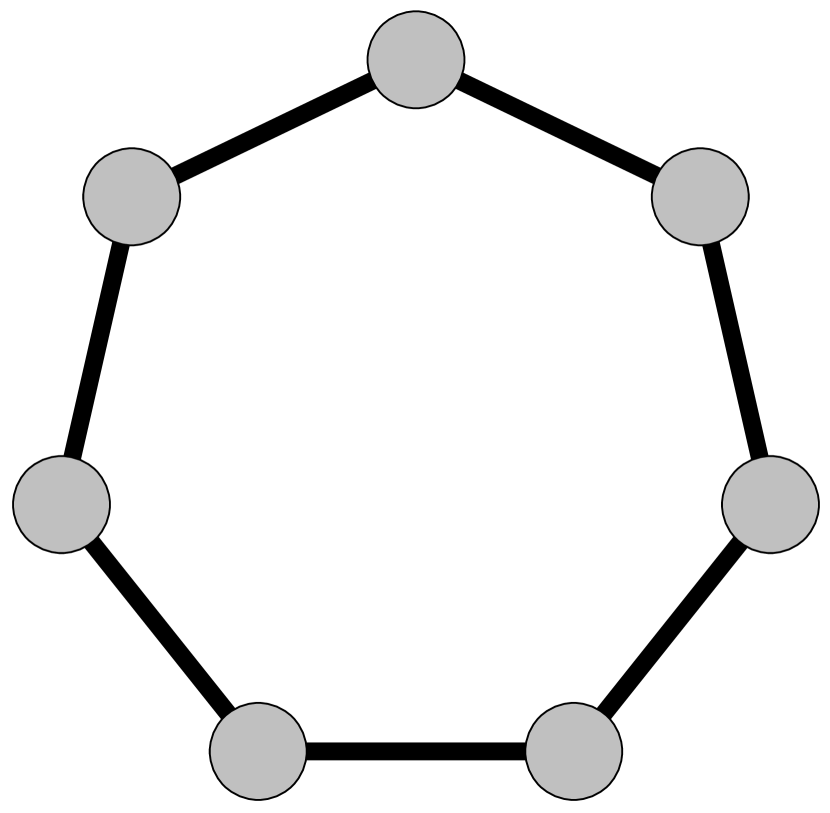
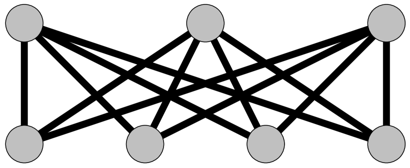
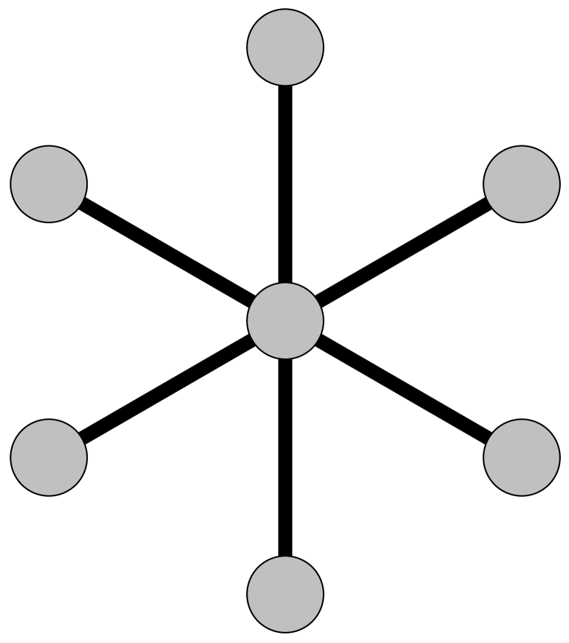
Figure 2: A 666-star, a 777-cycle, and the complete bipartite graph K3,4subscript𝐾34K_{3,4}. If 𝒢0subscript𝒢0\mathcal{G}_{0} is the 777-star and 𝒢1subscript𝒢1\mathcal{G}_{1} is the 777-cycle, then Π=S7Πsubscript𝑆7\Pi=S_{7}. If 𝒢0subscript𝒢0\mathcal{G}_{0} is the 7-star and 𝒢1=K3,4subscript𝒢1subscript𝐾34\mathcal{G}_{1}=K_{3,4}, then ΠS7Πsubscript𝑆7\Pi\neq S_{7}.

4.1 The star graph as 𝒢0subscript𝒢0\mathcal{G}_{0}

First, let 𝒢0subscript𝒢0\mathcal{G}_{0} be the star graph on n𝑛n vertices. Without loss of generality, let vertex 111 be the center vertex. Note that Π0Sn1subscriptΠ0subscript𝑆𝑛1\Pi_{0}\cong S_{n-1}. In fact, Π10=SnsubscriptΠ10subscript𝑆𝑛\Pi_{10}=S_{n} whenever Π1subscriptΠ1\Pi_{1} contains permutations mapping vertex 111 to any other vertex, which is equivalent to the definition of vertex transitivity. We summarize this observation in the following corollary:

Corollary 2.

Let 𝒢0subscript𝒢0\mathcal{G}_{0} be the star graph and suppose 𝒢1subscript𝒢1\mathcal{G}_{1} is vertex-transitive. Let πUniform(Sn)similar-to𝜋Uniformsubscript𝑆𝑛\pi\sim\text{Uniform}(S_{n}), and suppose S𝑆S is a Π1subscriptΠ1\Pi_{1}-invariant statistic. Then S()=dS(π)superscript𝑑𝑆𝑆𝜋S(\mathcal{I})\stackrel{{\scriptstyle d}}{{=}}S(\pi\mathcal{I}) under the null hypothesis, and the permutation test described in Algorithm 1 controls the Type I error at level α𝛼\alpha. A similar result holds when 𝒢1subscript𝒢1\mathcal{G}_{1} is the star graph and 𝒢0subscript𝒢0\mathcal{G}_{0} is vertex-transitive.

We now turn to risk bounds. Before we present the bounds, we provide some motivation. When β𝛽\beta is small, the two hypothesis spaces are close together, so the risk will be large; thus, we focus instead on the regime of moderate to large β𝛽\beta. When the null hypothesis is true, the infection still looks uniformly random when viewing 𝒢1subscript𝒢1\mathcal{G}_{1}, as stated in Corollary 1. Using a standard concentration bound, we then may verify that tαsubscript𝑡𝛼t_{\alpha} is O(k2/n+k)𝑂superscript𝑘2𝑛𝑘O(k^{2}/n+\sqrt{k}), where the two terms correspond to the expected value and the variance of W1()subscript𝑊1W_{1}(\mathcal{I}) under the null. When the alternative is true, the infected vertices should induce a connected subgraph of 𝒢1subscript𝒢1\mathcal{G}_{1}, with high probability. Thus, the expected value of W1()subscript𝑊1W_{1}(\mathcal{I}) is Ω(k)Ω𝑘\Omega(k). Finally, we use another standard concentration bound to obtain an upper bound on the probability that W1()tαsubscript𝑊1subscript𝑡𝛼W_{1}(\mathcal{I})\leq t_{\alpha} under the alternative.

Recall that all the vertices of a vertex-transitive graph have the same degree, which we denote by D𝐷D. It is natural that the risk depends on D𝐷D, since larger values of D𝐷D allow for more variation in W1()subscript𝑊1W_{1}(\mathcal{I}). Let Nt,minsubscript𝑁𝑡N_{t,\min} denote the minimum possible cut between the t𝑡t infected vertices and nt𝑛𝑡n-t uninfected vertices at time t𝑡t. We define the function

H(β)=m=1k1βnm+βNt,min.𝐻𝛽superscriptsubscriptproduct𝑚1𝑘1𝛽𝑛𝑚𝛽subscript𝑁𝑡H(\beta)=\prod_{m=1}^{k-1}\frac{\beta}{n-m+\beta N_{t,\min}}.

We also define a cascade on k𝑘k vertices to be a surjective map f:𝒱{0,,k}:𝑓𝒱0𝑘f:\mathcal{V}\to\{0,\ldots,k\}, such that

  • (i)

    v𝑣v is uninfected when f(v)=0𝑓𝑣0f(v)=0,

  • (ii)

    v𝑣v is the ithsuperscript𝑖thi^{\text{th}} vertex infected when f(v)=i𝑓𝑣𝑖f(v)=i, and

  • (iii)

    if f(v)=i𝑓𝑣𝑖f(v)=i, then v𝑣v must be adjacent to one of the first i1𝑖1i-1 infected nodes.

Let 𝒞k(u,v)subscript𝒞𝑘𝑢𝑣\mathcal{C}_{k}(u,v) denote the set of cascades on k𝑘k vertices such that both u𝑢u and v𝑣v are infected, and let Ck:=min(u,v)1|𝒞k(u,v)|assignsubscript𝐶𝑘subscript𝑢𝑣subscript1subscript𝒞𝑘𝑢𝑣C_{k}:=\min_{(u,v)\in\mathcal{E}_{1}}|\mathcal{C}_{k}(u,v)|. We have the following bound:

Proposition 1.

Suppose 𝒢1subscript𝒢1\mathcal{G}_{1} is a connected vertex-transitive graph with degree D𝐷D. Let ψW,αsubscript𝜓𝑊𝛼\psi_{W,\alpha} be the level-α𝛼\alpha permutation test based on the edges-within statistic W1subscript𝑊1W_{1}. Then

Rk,0(ψW,α,β)α+exp{2kD2(D2CkH(β)Dk(k1)2(n1)kD22log1α)2}.subscript𝑅𝑘0subscript𝜓𝑊𝛼𝛽𝛼2𝑘superscript𝐷2superscript𝐷2subscript𝐶𝑘𝐻𝛽𝐷𝑘𝑘12𝑛1𝑘superscript𝐷221𝛼2\displaystyle\begin{aligned} R_{k,0}(\psi_{W,\alpha},\beta)\leq\alpha+\exp\left\{-\frac{2}{kD^{2}}\left(\frac{D}{2}C_{k}H(\beta)-\frac{Dk(k-1)}{2(n-1)}-\sqrt{\frac{kD^{2}}{2}\log\frac{1}{\alpha}}\right)^{2}\right\}.\end{aligned}
Remark 3.

Note that H(β)𝐻𝛽H(\beta) is increasing in β𝛽\beta, so the risk bound in Proposition 1 decreases as β𝛽\beta increases. This agrees with intuition, since higher values of β𝛽\beta correspond to a higher chance that the infection propagates via edges rather than by random infections. Thus, the graphs 𝒢0subscript𝒢0\mathcal{G}_{0} and 𝒢1subscript𝒢1\mathcal{G}_{1} should be easier to distinguish.

For a cycle graph with k<n/2𝑘𝑛2k<n/2, we have the following result:

Corollary 3.

Let 𝒢1subscript𝒢1\mathcal{G}_{1} be the n𝑛n-cycle. Then Ck=(k1)2k1subscript𝐶𝑘𝑘1superscript2𝑘1C_{k}=(k-1)2^{k-1} and D=2𝐷2D=2, so

Rk,0(ψW,α,β)α+exp{12k((k1)2k1m=1k1βnm+2βk(k1)n12klog(1α))2}.\displaystyle\begin{aligned} R_{k,0}(\psi_{W,\alpha},\beta)&\leq\alpha+\exp\Bigg{\{}-\frac{1}{2k}\Bigg{(}(k-1)2^{k-1}\prod_{m=1}^{k-1}\frac{\beta}{n-m+2\beta}\\ &\qquad-\frac{k(k-1)}{n-1}-\sqrt{2k\log\left(\frac{1}{\alpha}\right)}\Bigg{)}^{2}\Bigg{\}}.\end{aligned}

In particular, if α=exp(Ck/2)𝛼𝐶𝑘2\alpha=\exp(-Ck/2) and k/n+C1ϵ𝑘𝑛𝐶1italic-ϵk/n+C\leq 1-\epsilon for some C>0𝐶0C>0 and ϵ>0italic-ϵ0\epsilon>0, then there exist C,C′′>0superscript𝐶superscript𝐶′′0C^{\prime},C^{\prime\prime}>0 such that

limβRk,0(ψW,α,β)Cexp(C′′k).subscript𝛽subscript𝑅𝑘0subscript𝜓𝑊𝛼𝛽superscript𝐶superscript𝐶′′𝑘\lim_{\beta\rightarrow\infty}R_{k,0}(\psi_{W,\alpha},\beta)\leq C^{\prime}\exp(-C^{\prime\prime}k).

The last statement reveals that as β𝛽\beta\to\infty, the risk will vanish for sufficiently large values of k𝑘k. However, if the fraction k/n𝑘𝑛k/n of infected nodes becomes too large, the two hypotheses are again difficult to distinguish.

4.2 The star graph as 𝒢1subscript𝒢1\mathcal{G}_{1}

We now consider the case when 𝒢1subscript𝒢1\mathcal{G}_{1} is the star graph on n𝑛n vertices. Again, let vertex 111 denote the center of the star. Perhaps unsurprisingly, it turns out that the maximum likelihood estimator and a test based on the edges-within statistic reduce to the same decision rule, depending on whether vertex 111 is included in the infected set:

Proposition 2.

Let c=0𝑐0c=0. Suppose 𝒢0subscript𝒢0\mathcal{G}_{0} is the empty graph. Maximum likelihood estimation is equivalent to the center indicator test C=𝟏{1=1}𝐶1subscript11C=\mathbf{1}\{\mathcal{I}_{1}=1\}, which is in turn equivalent to permutation testing at level α𝛼\alpha based on the edges-within statistic W1subscript𝑊1W_{1}, when αk/n𝛼𝑘𝑛\alpha\geq k/n.

Risk bounds for hypothesis testing based on C𝐶C are relatively easy to compute when 𝒢0subscript𝒢0\mathcal{G}_{0} is the empty graph. Corollary 1 implies that such bounds hold for permutation testing when 𝒢0subscript𝒢0\mathcal{G}_{0} is any vertex-transitive graph, from which we may derive the following result:

Proposition 3.

Suppose 𝒢0subscript𝒢0\mathcal{G}_{0} is a vertex-transitive graph. The risk of the center indicator test on the star graph on n𝑛n vertices satisfies the following bounds:

Rk,0(PC,β)kn+exp(k+βk(k1)/2nk),subscript𝑅𝑘0subscript𝑃𝐶𝛽𝑘𝑛𝑘𝛽𝑘𝑘12𝑛𝑘R_{k,0}(P_{C},\beta)\geq\frac{k}{n}+\exp\left(-\frac{k+\beta k(k-1)/2}{n-k}\right),

and

Rk,0(PC,β){kn+exp(k+βk(k1)/2(nk+1)+(k1)β),if β1,kn+exp(k+βk(k1)/2n),if β<1.subscript𝑅𝑘0subscript𝑃𝐶𝛽cases𝑘𝑛𝑘𝛽𝑘𝑘12𝑛𝑘1𝑘1𝛽if 𝛽1𝑘𝑛𝑘𝛽𝑘𝑘12𝑛if 𝛽1R_{k,0}(P_{C},\beta)\leq\begin{cases}\frac{k}{n}+\exp\left(-\frac{k+\beta k(k-1)/2}{(n-k+1)+(k-1)\beta}\right),&\text{if }\beta\geq 1,\\ \frac{k}{n}+\exp\left(-\frac{k+\beta k(k-1)/2}{n}\right),&\text{if }\beta<1.\end{cases}

Again, we can interpret the behavior of the risk bounds in terms of the fraction of infected vertices k/n𝑘𝑛k/n. When β𝛽\beta is fixed, the bound is k/n+exp(Θ(βk2/n))𝑘𝑛Θ𝛽superscript𝑘2𝑛k/n+\exp\left(\Theta\left(-\beta k^{2}/n\right)\right); thus, if we consider the size of the graph to be growing, we require k/n0𝑘𝑛0k/n\to 0 and k2/nsuperscript𝑘2𝑛k^{2}/n\to\infty in order to have vanishing risk. The first condition suggests that k𝑘k cannot be large enough to randomly infect the center of the star under the null. The intuition for the latter condition is that under the alternative, each infected leaf attempts to infect the center of the star at successive time steps. This leads to at most k(k1)/2𝑘𝑘12k(k-1)/2 infection attempts, and when the strength of these attempts is large enough, the center is infected with high probability.

5 A closer look at test statistics

It is natural to wonder which of the invariant statistics leads to the best statistical test, or even whether it is reasonable to focus our attention on invariant statistics. We address the first question by showing a rough equivalence of likelihood ratio testing to tests based on the edges-within statistic. For the second question, we derive some results motivated by the Hunt-Stein theory of hypothesis testing.

5.1 Likelihood ratio and edges-within

As noted earlier, the edges-within statistic appears in the probability density function of the 010101-Ising model: (J)=W(J)𝐽𝑊𝐽\mathcal{H}(J)=-W(J). Thus, a test based on a likelihood calculation may be equivalently expressed in terms of the edges-within statistic.

Turning to the stochastic spreading model, we now show that W1subscript𝑊1W_{1} arises as the first-order coefficient in the series expansion of the likelihood with respect to β𝛽\beta. This is somewhat reminiscent of the use of signed triangles in the random graph testing literature [4, 5, 10], which appears in the latter two cases as a first-order approximation to the asymptotic distribution of the log-likelihood. Furthermore, we will see that when considering the likelihood ratio of a test with a specific type of composite null hypothesis against the simple alternative 𝔊1={𝒢1}subscript𝔊1subscript𝒢1\mathfrak{G}_{1}=\{\mathcal{G}_{1}\}, the edges-within statistic W1subscript𝑊1W_{1} also appears as the first-order coefficient of the likelihood ratio. These approximations are quite attractive, since as noted earlier, computing the likelihood ratio would require summing over k!𝑘k! different infection paths and is itself intractable.

Before stating the main result, we introduce some additional notation. Let L(𝒢,β;J)𝐿𝒢𝛽𝐽L(\mathcal{G},\beta;J) denote the likelihood of infection J𝐽J under graph 𝒢𝒢\mathcal{G} and spreading parameter β𝛽\beta. Let

R(𝒢0,𝒢1,β;J)=L(𝒢1,β;J)L(𝒢0,β;J)𝑅subscript𝒢0subscript𝒢1𝛽𝐽𝐿subscript𝒢1𝛽𝐽𝐿subscript𝒢0𝛽𝐽R(\mathcal{G}_{0},\mathcal{G}_{1},\beta;J)=\frac{L(\mathcal{G}_{1},\beta;J)}{L(\mathcal{G}_{0},\beta;J)}

denote the likelihood ratio, and let 𝒢emptysubscript𝒢empty\mathcal{G}_{\text{empty}} denote the empty graph. Recall that Ntsubscript𝑁𝑡N_{t} denotes the number of edges connecting infected vertices to uninfected vertices at time t𝑡t.

Our main theorem shows the approximate equivalence between likelihood ratio tests and thresholding the edges-within statistic in the case of simple hypothesis testing when the null graph is empty.

Theorem 3.

Consider the hypothesis test of 𝒢emptysubscript𝒢empty\mathcal{G}_{\text{empty}} versus 𝒢1subscript𝒢1\mathcal{G}_{1}. For an uncensored P𝔓(J)𝑃𝔓𝐽P\in\mathfrak{P}(J) in which k+c𝑘superscript𝑐k+c^{\prime} vertices are infected, define the function

Q(P)=t=1k+cNtn+1t.𝑄𝑃superscriptsubscript𝑡1𝑘superscript𝑐subscript𝑁𝑡𝑛1𝑡Q(P)=\sum_{t=1}^{k+c^{\prime}}\frac{N_{t}}{n+1-t}.

If c=0𝑐0c=0, we have

R(𝒢empty,𝒢1,β;J)=(1+βW1(J)+O(β2W1(J)2))(11k!P𝔓(J)βQ(P)).𝑅subscript𝒢emptysubscript𝒢1𝛽𝐽absent1𝛽subscript𝑊1𝐽𝑂superscript𝛽2subscript𝑊1superscript𝐽211𝑘subscript𝑃𝔓𝐽𝛽𝑄𝑃\displaystyle\begin{aligned} R(\mathcal{G}_{\text{empty}},\mathcal{G}_{1},\beta;J)&=\left(1+\beta W_{1}(J)+O(\beta^{2}W_{1}(J)^{2})\right)\left(1-\frac{1}{k!}\sum_{P\in\mathfrak{P}(J)}\beta Q(P)\right).\end{aligned}

If c>0𝑐0c>0, we have

R(𝒢empty,𝒢1,β;J)=J𝒰(J)D(β,k,c,|J|)(1+βW1(J)+O(β2W1(J)2))×(11|J|!P𝔓(J)O(βQ(P))),𝑅subscript𝒢emptysubscript𝒢1𝛽𝐽absentsubscriptsuperscript𝐽𝒰𝐽𝐷𝛽𝑘𝑐superscript𝐽1𝛽subscript𝑊1superscript𝐽𝑂superscript𝛽2subscript𝑊1superscriptsuperscript𝐽2missing-subexpressionabsent11superscript𝐽subscript𝑃𝔓superscript𝐽𝑂𝛽𝑄𝑃\displaystyle\begin{aligned} R(\mathcal{G}_{\text{empty}},\mathcal{G}_{1},\beta;J)&=\sum_{J^{\prime}\in\mathcal{U}(J)}D(\beta,k,c,|J^{\prime}|)\left(1+\beta W_{1}(J^{\prime})+O(\beta^{2}W_{1}(J^{\prime})^{2})\right)\\ &\qquad\times\left(1-\frac{1}{|J^{\prime}|!}\sum_{P\in\mathfrak{P}(J^{\prime})}O(\beta Q(P))\right),\end{aligned}

where

D(β,k,c,r):=(nkc)(Z1(β)(nc)(nr))1.assign𝐷𝛽𝑘𝑐𝑟binomial𝑛𝑘𝑐superscriptsubscript𝑍1𝛽binomial𝑛𝑐binomial𝑛𝑟1D(\beta,k,c,r):=\binom{n}{k\;\;c}\left(Z_{1}(\beta)\binom{n}{c}\binom{n}{r}\right)^{-1}.

Thus, Theorem 3 shows that when c=0𝑐0c=0, the edges-within statistic W1()subscript𝑊1W_{1}(\mathcal{I}) is the leading term of the likelihood ratio expanded as a function of β𝛽\beta. When c>0𝑐0c>0, the expression is somewhat more complicated, since the number of edges within the (uncensored) infection subgraph may differ depending on the statuses of censored vertices. The first-order term then equals the value of the edges-within statistic averaged over all possible infection vectors giving rise to the censored vector J𝐽J.

Remark 4.

Note that even if the likelihood ratio converges to its first-order approximation 1+βW11𝛽subscript𝑊11+\beta W_{1} for some sequence of parameters, this does not ensure that W1subscript𝑊1W_{1} will always lead to a useful test. For instance, in the case that 𝒢1subscript𝒢1\mathcal{G}_{1} is a star graph, the condition βW10𝛽subscript𝑊10\beta W_{1}\to 0 and the conditions for asymptotically vanishing risk are incompatible. As discussed in Section 4.2, the latter conditions require k/n0𝑘𝑛0k/n\to 0 and βk2/n𝛽superscript𝑘2𝑛\beta k^{2}/n\to\infty. Since W1subscript𝑊1W_{1} may take on the value k1𝑘1k-1, requiring that βW1,k/n0𝛽subscript𝑊1𝑘𝑛0\beta W_{1},k/n\to 0 would imply that βk2/n0𝛽superscript𝑘2𝑛0\beta k^{2}/n\to 0, as well.

Finally, to obtain a test between two non-empty graphs, we use the simple relation

R(𝒢0,𝒢1,β;)=R(𝒢empty,𝒢1,β;)R(𝒢empty,𝒢0,β;).𝑅subscript𝒢0subscript𝒢1𝛽𝑅subscript𝒢emptysubscript𝒢1𝛽𝑅subscript𝒢emptysubscript𝒢0𝛽R(\mathcal{G}_{0},\mathcal{G}_{1},\beta;\mathcal{I})=\frac{R(\mathcal{G}_{\text{empty}},\mathcal{G}_{1},\beta;\mathcal{I})}{R(\mathcal{G}_{\text{empty}},\mathcal{G}_{0},\beta;\mathcal{I})}.

This expression depends on both W0subscript𝑊0W_{0} and W1subscript𝑊1W_{1}. However, cases exist where the expression only depends on W1subscript𝑊1W_{1}. For example, in the case of a composite null hypothesis involving testing a graph topology, we may derive the following theorem:

Theorem 4.

If 𝔊0=Sn𝔊0subscript𝔊0subscript𝑆𝑛subscript𝔊0\mathfrak{G}_{0}=S_{n}\mathfrak{G}_{0}, then supθΘ0L(θ;J)subscriptsupremum𝜃subscriptΘ0𝐿𝜃𝐽\sup_{\theta\in\Theta_{0}}L(\theta;J) is constant over J𝐽J in 𝕀k,csubscript𝕀𝑘𝑐\mathbb{I}_{k,c}. Consequently, if we denote this constant by Dsuperscript𝐷D^{\prime}, we have

R(𝔊0,𝒢1,β;J)=1DR(𝒢empty,𝒢1,β;J).𝑅subscript𝔊0subscript𝒢1𝛽𝐽1superscript𝐷𝑅subscript𝒢emptysubscript𝒢1𝛽𝐽R(\mathfrak{G}_{0},\mathcal{G}_{1},\beta;J)=\frac{1}{D^{\prime}}R(\mathcal{G}_{\text{empty}},\mathcal{G}_{1},\beta;J).

In conjunction with Theorem 3, Theorem 4 shows that we may again extract W1subscript𝑊1W_{1} as the leading term in the expansion for the likelihood ratio. Another immediate corollary is that it is not possible to directly test between two unlabeled topologies, since the likelihoods for both hypotheses would be constant.

5.2 Hunt-Stein theory for graph testing

When conducting hypothesis tests, it is natural to consider maximin tests, i.e., tests that maximize the minimum power over the space of alternative hypotheses. A standard way to do this for invariant tests is via the Hunt-Stein theorem [33]. The goal of this section is to demonstrate that a version of the Hunt-Stein theorem also holds for the graph testing problem, further motivating our use of hypothesis testing via Π1subscriptΠ1\Pi_{1}-invariant test statistics. The results in this subsection hold for general null and alternative parameter spaces Θ0=𝔊0×+subscriptΘ0subscript𝔊0subscript\Theta_{0}=\mathfrak{G}_{0}\times\mathbb{R}_{+} and Θ1=𝔊1×+subscriptΘ1subscript𝔊1subscript\Theta_{1}=\mathfrak{G}_{1}\times\mathbb{R}_{+}. Let Θ:=Θ0Θ1assignΘsubscriptΘ0subscriptΘ1\Theta:=\Theta_{0}\cup\Theta_{1}.

Recall that a critical function φ𝜑\varphi outputs a value in {0,1}01\{0,1\} for each observed infection vector \mathcal{I}, corresponding to the selected hypothesis. A test based on φ𝜑\varphi is ΠΠ\Pi-invariant if φ(π)=φ()𝜑𝜋𝜑\varphi(\pi\mathcal{I})=\varphi(\mathcal{I}) for all πΠ𝜋Π\pi\in\Pi. Furthermore, the test is maximin at level α𝛼\alpha if

maxθΘ0𝔼θ[φ()]α,subscript𝜃subscriptΘ0subscript𝔼𝜃delimited-[]𝜑𝛼\max_{\theta\in\Theta_{0}}\mathbb{E}_{\theta}[\varphi(\mathcal{I})]\leq\alpha, (8)

and the value of

minθΘ1𝔼θ[φ()]subscript𝜃subscriptΘ1subscript𝔼𝜃delimited-[]𝜑\min_{\theta\in\Theta_{1}}\mathbb{E}_{\theta}[\varphi(\mathcal{I})]

is maximized among all tests φsuperscript𝜑\varphi^{\prime} satisfying inequality (8).

Analogous to canonical Hunt-Stein results, we will assume that both 𝔊0subscript𝔊0\mathfrak{G}_{0} and 𝔊1subscript𝔊1\mathfrak{G}_{1} are invariant under the same group of transformations, which in our setting is Π1subscriptΠ1\Pi_{1}. A natural case where this condition is satisfied is when 𝔊1subscript𝔊1\mathfrak{G}_{1} consists of a single graph 𝒢1subscript𝒢1\mathcal{G}_{1} and 𝔊0subscript𝔊0\mathfrak{G}_{0} consists of all permutations of a graph 𝒢0subscript𝒢0\mathcal{G}_{0}. For instance, suppose 𝒢1subscript𝒢1\mathcal{G}_{1} is a cycle graph; if we wish to test a null hypothesis involving a star graph 𝒢0subscript𝒢0\mathcal{G}_{0}, we can define 𝔊0subscript𝔊0\mathfrak{G}_{0} to include all permutations of 𝒢0subscript𝒢0\mathcal{G}_{0} under Π1subscriptΠ1\Pi_{1}, as well, which yields n𝑛n stars with different center vertices.

Theorem 5 (Hunt-Stein for graph testing).

Let ΠΠ\Pi be a group of transformations on \mathcal{I}, and let Θ0subscriptΘ0\Theta_{0}, and Θ1subscriptΘ1\Theta_{1} be such that ΠΘ0=Θ0ΠsubscriptΘ0subscriptΘ0\Pi\Theta_{0}=\Theta_{0} and ΠΘ1=Θ1ΠsubscriptΘ1subscriptΘ1\Pi\Theta_{1}=\Theta_{1}. If there exists a level-α𝛼\alpha test φsuperscript𝜑\varphi^{*} maximizing infθΘ𝔼θ[φ()]subscriptinfimum𝜃Θsubscript𝔼𝜃delimited-[]𝜑\inf_{\theta\in\Theta}\mathbb{E}_{\theta}[\varphi(\mathcal{I})], then there also exists a ΠΠ\Pi-invariant test with this property, defined by

ψ(J)=1|Π|πΠφ(πJ).superscript𝜓𝐽1Πsubscript𝜋Πsuperscript𝜑𝜋𝐽\psi^{*}(J)=\frac{1}{|\Pi|}\sum_{\pi\in\Pi}\varphi^{*}(\pi J).

Thus, for composite tests in which Θ0subscriptΘ0\Theta_{0} and Θ1subscriptΘ1\Theta_{1} are both Π1subscriptΠ1\Pi_{1}-invariant, whenever we can find a maximin critical function φ𝜑\varphi, we can also find a maximin Π1subscriptΠ1\Pi_{1}-invariant critical function. Note, however, that one could likely do better than a Π1subscriptΠ1\Pi_{1}-invariant test when 𝔊0subscript𝔊0\mathfrak{G}_{0} is not Π1subscriptΠ1\Pi_{1}-invariant, such as in the case of a star with a fixed center.

6 General testing procedures

Our permutation testing procedure exploits graph symmetries to great effect; however, the strong symmetry assumptions may sometimes be prohibitive. One particular case would be testing a graph 𝒢𝒢\mathcal{G} against a “close” variant 𝒢superscript𝒢\mathcal{G}^{\prime}, such as a subgraph of 𝒢𝒢\mathcal{G} with a few edges removed.

Consider testing the hypotheses

H0:SSM(𝒢0,β0) for β0𝔅0,H1:SSM(𝒢1,β1) for β1𝔅1.subscript𝐻0:absentsimilar-toSSMsubscript𝒢0subscript𝛽0 for subscript𝛽0subscript𝔅0subscript𝐻1:absentsimilar-toSSMsubscript𝒢1subscript𝛽1 for subscript𝛽1subscript𝔅1\displaystyle\begin{aligned} H_{0}&:\mathcal{I}\sim\text{SSM}(\mathcal{G}_{0},\beta_{0})\text{ for }\beta_{0}\in\mathfrak{B}_{0},\\ H_{1}&:\mathcal{I}\sim\text{SSM}(\mathcal{G}_{1},\beta_{1})\text{ for }\beta_{1}\in\mathfrak{B}_{1}.\end{aligned}

We now propose and analyze a general testing procedure. The idea is straightforward: For a finite set Dsubscript𝐷\mathfrak{C}_{D}, define a discretization function FD:[0,)D:subscript𝐹𝐷0subscript𝐷F_{D}:[0,\infty)\to\mathfrak{C}_{D} such that

TV(0,β,0,FD(β))δ,TVsubscript0𝛽subscript0subscript𝐹𝐷𝛽𝛿\text{TV}\left(\mathbb{P}_{0,\beta},\mathbb{P}_{0,F_{D}(\beta)}\right)\leq\delta, (9)

and 𝔅0,Dsubscript𝔅0𝐷\mathfrak{B}_{0,D} = FD(𝔅0)subscript𝐹𝐷subscript𝔅0F_{D}(\mathfrak{B}_{0}). We then simulate a sufficient number of infection processes with the parameters (𝒢0,β0)subscript𝒢0subscript𝛽0(\mathcal{G}_{0},\beta_{0}) for β0subscript𝛽0\beta_{0} in 𝔅0,Dsubscript𝔅0𝐷\mathfrak{B}_{0,D} to approximate the distribution for all parameter values in the null hypothesis, which allows us to perform tests or, alternatively, form confidence sets for the underlying graph structure. Although the idea is fairly simple, the appropriate discretization is somewhat lengthy to state; therefore, we defer further details on the discretization to Appendix C. In the remainder of the section, we describe basic hypothesis tests and confidence interval algorithms.

6.1 Hypothesis testing algorithm

With a discretization satisfying equation (9) in hand, it is straightforward to devise a simulation-based algorithm that controls the Type I error. This is summarized in Algorithm 3. Further details on algorithm parameters may be found in Appendix C, but briefly, we note that decreasing ϵitalic-ϵ\epsilon, δ𝛿\delta, or ξ𝜉\xi increases the size of the discretization and therefore the computational burden, while increasing the statistical power.

Input : Type I error tolerance α>0𝛼0\alpha>0, approximation parameters ϵitalic-ϵ\epsilon, δ𝛿\delta, and ξ𝜉\xi, observed infection vector \mathcal{I}, null graph 𝒢0subscript𝒢0\mathcal{G}_{0}, statistic S𝑆S, discretization 𝔅0,Dsubscript𝔅0𝐷\mathfrak{B}_{0,D} of size N𝑁N, discretization function FDsubscript𝐹𝐷F_{D}
1
2Define Nsims(12ϵ2+83ϵ)log1ξsubscript𝑁sims12superscriptitalic-ϵ283italic-ϵ1𝜉N_{\text{sims}}\geq\left(\frac{1}{2\epsilon^{2}}+\frac{8}{3\epsilon}\right)\log\frac{1}{\xi}
3For each β𝛽\beta in 𝔅0,Dsubscript𝔅0𝐷\mathfrak{B}_{0,D}, simulate an infection Nsimssubscript𝑁simsN_{\text{sims}} times on 𝒢0subscript𝒢0\mathcal{G}_{0} to obtain the approximate 1(αγϵ)1𝛼𝛾italic-ϵ1-(\alpha-\gamma-\epsilon) quantile t^αδξϵ,βsubscript^𝑡𝛼𝛿𝜉italic-ϵ𝛽\hat{t}_{\alpha-\delta-\xi-\epsilon,\beta}
4Compute t^αδξϵ=maxβ𝔅0,Dt^αγϵ,βsubscript^𝑡𝛼𝛿𝜉italic-ϵsubscript𝛽subscript𝔅0𝐷subscript^𝑡𝛼𝛾italic-ϵ𝛽\hat{t}_{\alpha-\delta-\xi-\epsilon}=\max_{\beta\in\mathfrak{B}_{0,D}}\hat{t}_{\alpha-\gamma-\epsilon,\beta}
Reject the null hypothesis if S()>t^αδξϵ𝑆subscript^𝑡𝛼𝛿𝜉italic-ϵS(\mathcal{I})>\hat{t}_{\alpha-\delta-\xi-\epsilon}
Algorithm 3 One-Statistic Test
Theorem 6.

Let 𝒢0subscript𝒢0\mathcal{G}_{0} be a graph and S𝑆S be a statistic. Let α>0𝛼0\alpha>0 be given, and set ϵ<αδξitalic-ϵ𝛼𝛿𝜉\epsilon<\alpha-\delta-\xi. Then Algorithm 3 with a discretization function satisfying equation (9) controls the Type I error at level α𝛼\alpha.

We prove this result in Appendix H.

Remark 5.

While Theorem 6 proves the correctness of simulation tests, we still need to address further statistical and computational details. Statistically, we are interested in tests with good power. Since the test statistic S𝑆S may be arbitrary, we cannot make statements about the power of the procedure in general; for example, a constant statistic S𝑆S would have a Type I error of 00 and a Type II error of 111. Nonetheless, in addition to testing a broader class of graphs, we may also use many more statistics than the edges-within statistic. However, this does not include the likelihood ratio, even though the likelihood ratio suffers from the further problem of being generally uncomputable, because the likelihood statistic is usually a function of the parameters β0subscript𝛽0\beta_{0} and β1subscript𝛽1\beta_{1}, as well.

We also make one remark regarding the relation between Algorithm 2 and Algorithm 3. The question of how large to make Nsimssubscript𝑁simsN_{\text{sims}} is more important in the case of general graphs because the size of the discretization N𝑁N is usually quite large, making increasing Nsimssubscript𝑁simsN_{\text{sims}} costly. However, if we wished to be more precise for Algorithm 2, note that Theorem 6 provides the necessary error framework. To account for error properly in Algorithm 2, we would choose the parameters of Algorithm 3 with δ=0𝛿0\delta=0, 𝔅0,D={0}subscript𝔅0𝐷0\mathfrak{B}_{0,D}=\{0\}, and, consequently, N=1𝑁1N=1.

6.2 Confidence set algorithm

A convenient consequence of the general discretization procedure is that we can invert the tests to obtain confidence sets for both the graph and the parameter β𝛽\beta. To this end, we provide a slightly modified algorithm to compute confidence sets, matching the test that we have given. In analog with Algorithm 3, we provide the following confidence set algorithm in Algorithm 4.

Input : Type I error tolerance α>0𝛼0\alpha>0, approximation parameters ϵitalic-ϵ\epsilon, δ𝛿\delta, and ξ𝜉\xi, observed infection vector \mathcal{I}, set of graphs 𝔊𝔊\mathfrak{G}, statistic S𝑆S, discretization 𝔅𝒢,Dsubscript𝔅𝒢𝐷\mathfrak{B}_{\mathcal{G},D} of size N𝒢subscript𝑁𝒢N_{\mathcal{G}} for each 𝒢𝒢\mathcal{G} in 𝔊𝔊\mathfrak{G}, discretization functions F𝒢,Dsubscript𝐹𝒢𝐷F_{\mathcal{G},D}
1
2Define Nsims(12ϵ2+83ϵ)log1ξsubscript𝑁sims12superscriptitalic-ϵ283italic-ϵ1𝜉N_{\text{sims}}\geq\left(\frac{1}{2\epsilon^{2}}+\frac{8}{3\epsilon}\right)\log\frac{1}{\xi}
3For each β𝛽\beta in 𝔅𝒢,Dsubscript𝔅𝒢𝐷\mathfrak{B}_{\mathcal{G},D}, simulate an infection Nsimssubscript𝑁simsN_{\text{sims}} times on 𝒢𝒢\mathcal{G} to obtain the approximate 1(αδξϵ)1𝛼𝛿𝜉italic-ϵ1-(\alpha-\delta-\xi-\epsilon) quantile t^αδξϵ,βsubscript^𝑡𝛼𝛿𝜉italic-ϵ𝛽\hat{t}_{\alpha-\delta-\xi-\epsilon,\beta}
4Define the discrete confidence sets
C𝒢,D:={β𝔅D:S()t^αδξϵ,β}assignsubscript𝐶𝒢𝐷conditional-set𝛽subscript𝔅𝐷𝑆subscript^𝑡𝛼𝛿𝜉italic-ϵ𝛽C_{\mathcal{G},D}:=\left\{\beta\in\mathfrak{B}_{D}:S(\mathcal{I})\leq\hat{t}_{\alpha-\delta-\xi-\epsilon,\beta}\right\}
Return the confidence set C=𝒢𝔊(𝒢,F𝒢,D1(C𝒢,D))𝐶subscript𝒢𝔊𝒢superscriptsubscript𝐹𝒢𝐷1subscript𝐶𝒢𝐷C=\bigcup_{\mathcal{G}\in\mathfrak{G}}\left(\mathcal{G},F_{\mathcal{G},D}^{-1}(C_{\mathcal{G},D})\right)
Algorithm 4 One-Statistic Confidence Set
Corollary 4.

If for each 𝒢𝒢\mathcal{G} in 𝔊𝔊\mathfrak{G} the discretization 𝔅𝒢,Dsubscript𝔅𝒢𝐷\mathfrak{B}_{\mathcal{G},D} and discretization function F𝒢,Dsubscript𝐹𝒢𝐷F_{\mathcal{G},D} satisfy equation (9) and the approximation parameters are chosen as in Theorem 6, the set C𝐶C returned by Algorithm 4 is a (1α)1𝛼(1-\alpha)-confidence set.

7 Application to an HIV graph

Refer to caption
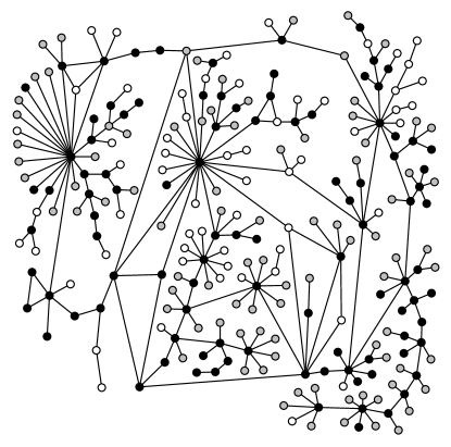
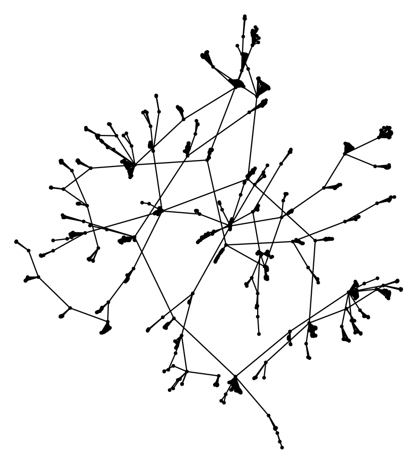
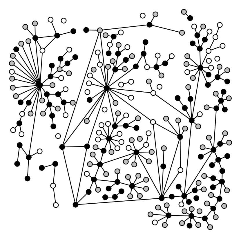
Figure 3: The HIV infection graph. Black vertices are infected, white vertices are uninfected, and gray vertices are censored. Edges represent sexual or injecting drug use relationships. Reproduced from Sexually Transmitted Infections, Potterat et al., 78, i159–i163, 2002, with permission from BMJ Publishing Group, Ltd.

Finally, we applied our permutation testing procedures to assess the explanatory power of an HIV network. We also examined two close variants of the network with our general graph methods. The network is constructed from the population of Colorado Springs from 1982–1989, and the observed infection statuses of individuals, obtained from the CDC and the HIV Counseling and Testing Center, is reported in [45]. For a visualization of the network, see Figure 3 above. The network was constructed from contact tracing for sexual and injecting drug partners; beginning in 1985, officials interviewed people testing positive for HIV for information to identify relevant partners.

7.1 Permutation results

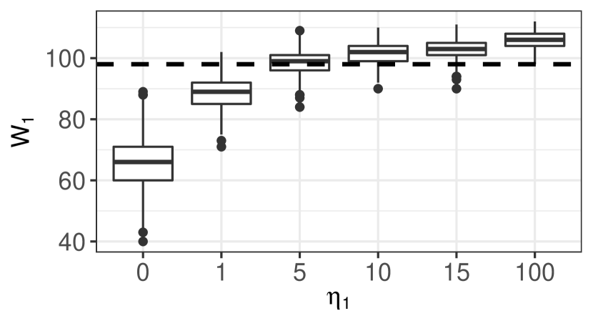
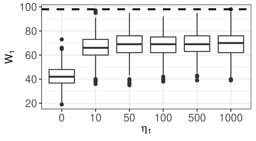
We first applied Algorithm 2 with the edges-within statistic W𝑊W, resulting in W()=98𝑊98W(\mathcal{I})=98. Based on Nsims=1000subscript𝑁sims1000N_{\text{sims}}=1000 randomly drawn permutations, we obtained an approximate p𝑝p-value of 0; i.e., none of the simulations yielded a value of W𝑊W of at least 989898. This should provide substantial evidence of the explanatory power of the graph. However, a closer examination of the network reveals that the censored nodes might not be chosen at random. To further validate this observation, we simulated our stochastic spreading model on the HIV graph, and computed W𝑊W for λ=1𝜆1\lambda=1 and various values of β𝛽\beta in [10,1000]101000[10,1000]. A boxplot is provided in Figure 4. In particular, none of the simulations produced a value of W𝑊W greater than or equal to 989898, and increasing β𝛽\beta even further seems to have little effect.
Refer to caption
Refer to caption
Figure 4: The distributions of W𝑊W for different values of β𝛽\beta on the HIV graph, based on 1000 simulations. The left plot corresponds to random censoring, whereas the right plot conditions on the censored nodes. The dashed line shows W1=98subscript𝑊198W_{1}=98, the value from the data. No β𝛽\beta appears to be consistent with the observed value W=98𝑊98W=98 in the randomized censoring model; such a value is more typical in the conditional censoring model.

Subsequently, we used Algorithm 7 of the Appendix with statistic W𝑊W, with the empty graph as the null. The approximate p𝑝p-value computed from 1000 simulations was again 0. However, simulating the stochastic spreading model on the HIV graph, conditioned on the censored nodes, leads to more reasonable values of W𝑊W. Boxplots for simulations corresponding to λ=1𝜆1\lambda=1 and β{0,1,5,10,15,100}𝛽0151015100\beta\in\{0,1,5,10,15,100\} are shown in the right-hand plot of Figure 4. Note that for moderate values of β𝛽\beta, the observed value 98 lies squarely within the range of the empirical distribution of W𝑊W. This suggests that the model which conditions on the censored nodes provides a better fit to the data.

Finally, note that neither of the algorithms from [39] produce meaningful conclusions. In the case of the TB algorithm, all positive integers d𝑑d lead to a threshold larger than the diameter of the graph, so the algorithm will always reject the null hypothesis. Similarly, the threshold for the TT algorithm is 779779779, which exceeds the weight of any spanning tree since the graph has only 250 vertices. The TB and TT algorithms both fail due to the closely-connected structure of HIV graph, which is a characteristic of many real-world networks, and the inability to select a good threshold.

7.2 General graph results

Here, we consider confidence sets for the pairs (𝒢,β)𝒢𝛽(\mathcal{G},\beta). Since our procedure relies on simulating a null distribution for a given pair of parameters, we cannot hope to construct the full confidence set, since enumerating all graphs for even small n𝑛n is difficult. However, we can use our procedure to test whether a particular graph lies in a given (1α)1𝛼(1-\alpha)-confidence set; we do this for a pair of graphs to demonstrate the applicability of the method.

For the confidence set algorithm, we use Algorithm 9. We set α=0.2𝛼0.2\alpha=0.2, with α0=α1=α/2subscript𝛼0subscript𝛼1𝛼2\alpha_{0}=\alpha_{1}=\alpha/2. We set the parameters ϵ=0.029italic-ϵ0.029\epsilon=0.029, ξ=0.001𝜉0.001\xi=0.001, and δ=0.02𝛿0.02\delta=0.02. For a discussion on choosing parameter values, see Appendix C. Our two statistics are W𝑊W and W𝑊-W, i.e., we wish to have two-sided confidence sets for the statistic W𝑊W. Finally, we restrict to the set 𝔅=[0,10]𝔅010\mathfrak{B}=[0,10] in computing the confidence set, since this leads to over 15,0001500015,000 values of β𝛽\beta for each of the two graphs we consider.

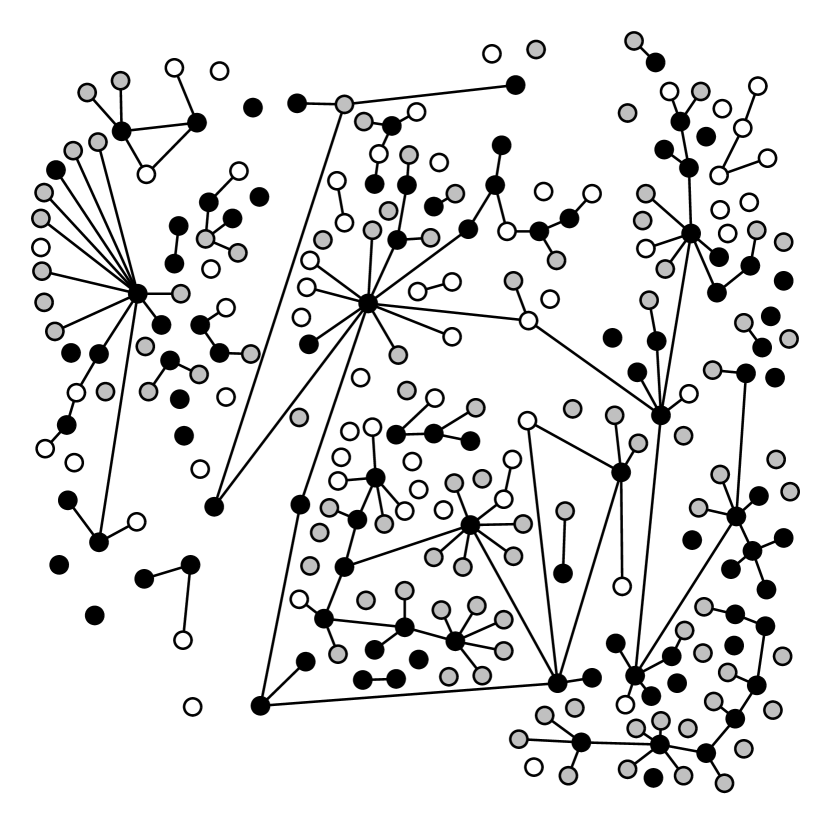
First, we consider a graph that we call “graph 25” or 𝒢25subscript𝒢25\mathcal{G}_{25}, since it is the HIV graph with 25 randomly-chosen edges removed. A picture is available in the left part of Figure 5.
Refer to caption
Refer to caption
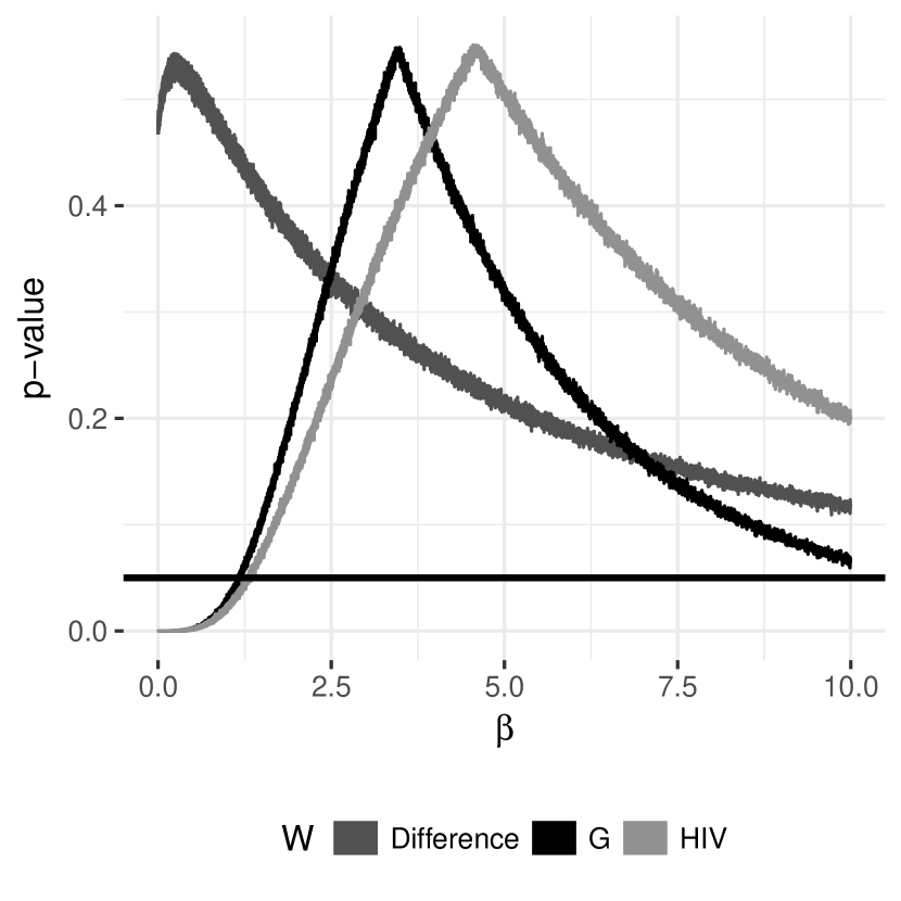
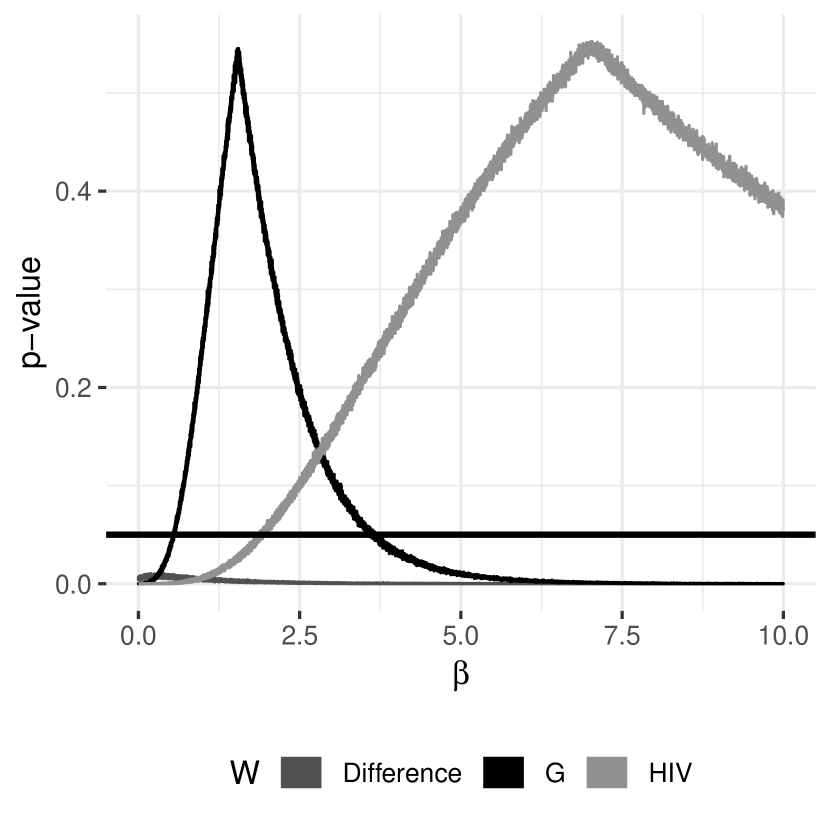
Figure 5: The graph 𝒢25subscript𝒢25\mathcal{G}_{25} used in computing the joint confidence set of (𝒢25,β)subscript𝒢25𝛽(\mathcal{G}_{25},\beta) and the p𝑝p-values for various statistics. The graph was formed from the HIV graph by removing 25 edges uniformly at random. Black vertices are infected, white vertices are uninfected, and gray vertices are censored. On the right, we have the p𝑝p-values as a function of β𝛽\beta for the HIV graph using the two-statistic test with different test statistics. The statistics are W𝒢25subscript𝑊subscript𝒢25W_{\mathcal{G}_{25}}, W𝒢HIVsubscript𝑊subscript𝒢HIVW_{\mathcal{G}_{\text{HIV}}}, and W𝒢25W𝒢HIVsubscript𝑊subscript𝒢25subscript𝑊subscript𝒢HIVW_{\mathcal{G}_{25}}-W_{\mathcal{G}_{\text{HIV}}}, and the p𝑝p-values for these are given by the black line, the light gray line, and the dark graph line respectively. Values of β𝛽\beta for which a curve is above the horizontal line at 0.050.050.05 are in the confidence set generated by the corresponding statistic.

For illustration, we consider two-sided tests for W𝒢25subscript𝑊subscript𝒢25W_{\mathcal{G}_{25}}, W𝒢HIVsubscript𝑊subscript𝒢HIVW_{\mathcal{G}_{\text{HIV}}}, and W𝒢25W𝒢HIVsubscript𝑊subscript𝒢25subscript𝑊subscript𝒢HIVW_{\mathcal{G}_{25}}-W_{\mathcal{G}_{\text{HIV}}}, i.e., the edges-within statistic computed with respect to 𝒢25subscript𝒢25\mathcal{G}_{25}, the edges-within statistic computed with respect to the HIV graph, and the difference of these statistics. The precise algorithm is Algorithm 9, given in the Appendix. The results are shown on the right in Figure 5. This figure is to be interpreted as follows: For each value of β𝛽\beta in 𝔅Dsubscript𝔅𝐷\mathfrak{B}_{D}, we perform many simulations to estimate the upper and lower percentiles p^𝒢,S(β,)subscript^𝑝𝒢𝑆𝛽\hat{p}_{\mathcal{G},S}(\beta,\mathcal{I}) and p^𝒢,S(β,)subscriptsuperscript^𝑝𝒢𝑆𝛽\hat{p}^{\prime}_{\mathcal{G},S}(\beta,\mathcal{I}) of the statistic S𝑆S, where

p^𝒢,S(β,)=1Nsimsi=1Nsims𝟏{S(Ii)S()}p^𝒢,S(β,)=1Nsimsi=1Nsims𝟏{S(Ii)S()}subscript^𝑝𝒢𝑆𝛽absent1subscript𝑁simssuperscriptsubscript𝑖1subscript𝑁sims1𝑆subscript𝐼𝑖𝑆subscriptsuperscript^𝑝𝒢𝑆𝛽absent1subscript𝑁simssuperscriptsubscript𝑖1subscript𝑁sims1𝑆subscript𝐼𝑖𝑆\displaystyle\begin{aligned} \hat{p}_{\mathcal{G},S}(\beta,\mathcal{I})&=\frac{1}{N_{\text{sims}}}\sum_{i=1}^{N_{\text{sims}}}\mathbf{1}\left\{S(I_{i})\leq S(\mathcal{I})\right\}\\ \hat{p}^{\prime}_{\mathcal{G},S}(\beta,\mathcal{I})&=\frac{1}{N_{\text{sims}}}\sum_{i=1}^{N_{\text{sims}}}\mathbf{1}\left\{S(I_{i})\geq S(\mathcal{I})\right\}\end{aligned}

and Iisubscript𝐼𝑖I_{i} are the simulated infections with parameter β𝛽\beta. Then, we plotted the minimum percentile qS(β)=min{p^𝒢,S(β,),p^𝒢,S(β,)}subscript𝑞𝑆𝛽subscript^𝑝𝒢𝑆𝛽subscriptsuperscript^𝑝𝒢𝑆𝛽q_{S}(\beta)=\min\left\{\hat{p}_{\mathcal{G},S}(\beta,\mathcal{I}),\hat{p}^{\prime}_{\mathcal{G},S}(\beta,\mathcal{I})\right\} against β𝛽\beta for three different statistics. Therefore, the approximate confidence set for β𝛽\beta given by S𝑆S consists of the β𝛽\beta for which the qS(β)subscript𝑞𝑆𝛽q_{S}(\beta) is above the horizontal line at 0.050.050.05. The precise confidence interval would be obtained by mapping back via FD1superscriptsubscript𝐹𝐷1F_{D}^{-1}, but rounding after two or three decimal places is sufficient here.

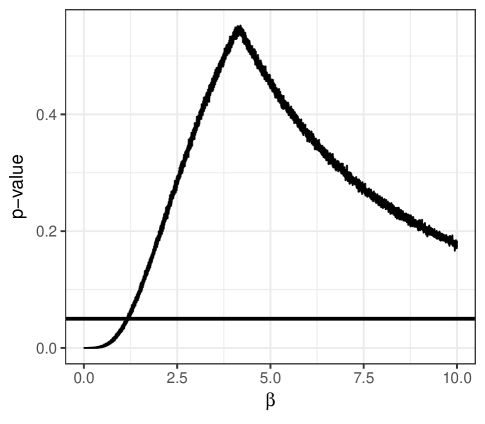
Note that the statistics W𝒢25subscript𝑊subscript𝒢25W_{\mathcal{G}_{25}} and W𝒢HIVsubscript𝑊subscript𝒢HIVW_{\mathcal{G}_{\text{HIV}}} lead to confidence sets for β𝛽\beta of approximately [1.14,10]1.1410[1.14,10] and [1.27,10]1.2710[1.27,10] respectively. On the other hand, the difference W𝒢25W𝒢HIVsubscript𝑊subscript𝒢25subscript𝑊subscript𝒢HIVW_{\mathcal{G}_{25}}-W_{\mathcal{G}_{\text{HIV}}} leads to the confidence interval [0,10]010[0,10]. This is unsurprising, since the 𝒢25subscript𝒢25\mathcal{G}_{25} and 𝒢HIVsubscript𝒢HIV\mathcal{G}_{\text{HIV}} are not too different. We now repeat this procedure on a different graph, 𝒢100subscript𝒢100\mathcal{G}_{100}, which has 100100100 edges removed from the HIV graph uniformly at random. Note that 𝒢100subscript𝒢100\mathcal{G}_{100} is a subgraph of 𝒢25subscript𝒢25\mathcal{G}_{25}. An image of the graph and the results of the analysis are shown in Figure 6. The major difference for 𝒢100subscript𝒢100\mathcal{G}_{100} is that no value of β𝛽\beta is included in the confidence set for the difference statistic W𝒢100W𝒢HIVsubscript𝑊subscript𝒢100subscript𝑊subscript𝒢HIVW_{\mathcal{G}_{100}}-W_{\mathcal{G}_{\text{HIV}}}. This is likely due to the fact that many edges exist in 𝒢HIVsubscript𝒢HIV\mathcal{G}_{\text{HIV}} between infected vertices that do not exist when simulating the distribution using 𝒢100subscript𝒢100\mathcal{G}_{100}. In short, for the values of β𝛽\beta from [0,10]010[0,10], we have found a non-trivial graph that is not in the confidence set of graphs given by the observed infection.
Refer to caption
Refer to caption
Figure 6: The graph 𝒢100subscript𝒢100\mathcal{G}_{100} used in computing the joint confidence set of (𝒢100,β)subscript𝒢100𝛽(\mathcal{G}_{100},\beta) and the p𝑝p-values for various statistics. The graph was formed from the HIV graph by removing 100 edges uniformly at random. Black vertices are infected, white vertices are uninfected, and gray vertices are censored. On the right, we have the p𝑝p-values as a function of β𝛽\beta for the HIV graph using the two-statistic test with different test statistics. The statistics are W𝒢100subscript𝑊subscript𝒢100W_{\mathcal{G}_{100}}, W𝒢HIVsubscript𝑊subscript𝒢HIVW_{\mathcal{G}_{\text{HIV}}}, and W𝒢25W𝒢HIVsubscript𝑊subscript𝒢25subscript𝑊subscript𝒢HIVW_{\mathcal{G}_{25}}-W_{\mathcal{G}_{\text{HIV}}}, and the p𝑝p-values for these are given by the black line, the light gray line, and the dark graph line respectively. Values of β𝛽\beta for which a curve is above the horizontal line at 0.050.050.05 are in the confidence set generated by the corresponding statistic.

8 Discussion

The results presented in our paper suggest several avenues for further research. Although we only considered two infection models and closely examined the stochastic spreading model, the permutation testing framework could be extended to other infection models, as well. As an extension of Ising models, one could consider other classes of Markov random fields. Toward network modeling, such tests would also be helpful for testing network structure, such as Erdős-Renyi networks versus networks with block structure. We have left open the question of whether a version of Theorem 1 holds in more generality. It would also be useful to devise a more interpretable or verifiable sufficient condition for the validity of the permutation test. Additionally, while our general graph methods can in principle be applied to any graph, it would be computationally prohibitive to do so for larger graphs. Thus, an open question is how to devise more efficient algorithms for testing general graph structures.

Acknowledgments

The authors thank Varun Jog, Dylan Small, and Miklos Racz for helpful comments and discussions. The authors also thank the AE and anonymous reviewers for their many insightful suggestions.

References

  • [1] R. Albert, H. Jeong, and A.-L. Barabási. Error and attack tolerance of complex networks. Nature, 406(6794):378–382, 2000.
  • [2] R. M. Anderson and R. M. May. Infectious Diseases of Humans: Dynamics and Control. Dynamics and Control. Oxford University Press, 1992.
  • [3] D. Angluin, J. Aspnes, and L. Reyzin. Network construction with subgraph connectivity constraints. Journal of Combinatorial Optimization, 29(2):418–432, 2015.
  • [4] D. Banerjee. Contiguity and non-reconstruction results for planted partition models: the dense case. Electronic Journal of Probability, 23, 2018.
  • [5] D. Banerjee and Z. Ma. Optimal hypothesis testing for stochastic block models with growing degrees. arXiv preprint arXiv:1705.05305, 2017.
  • [6] C. Borgs, M. Brautbar, J. Chayes, S. Khanna, and B. Lucier. The power of local information in social networks. Proceedings of the 8th International Workshop on Internet and Network Economics, pages 406–419, 2012.
  • [7] S. Boucheron, G. Lugosi, and P. Massart. Concentration Inequalities: a Nonasymptotic Theory of Independence. Oxford University Press, 2013.
  • [8] M. Brautbar and M. Kearns. Local algorithms for finding interesting individuals in large networks. Innovations in Theoretical Computer Science, 2010.
  • [9] S. Bubeck, L. Devroye, and G. Lugosi. Finding Adam in random growing trees. Random Structures & Algorithms, 50(2):158–172, 2017.
  • [10] S. Bubeck, J. Ding, R. Eldan, and M. Rácz. Testing for high-dimensional geometry in random graphs. Random Structures & Algorithms, 49(3):503–532, 2016.
  • [11] W. Chen, C. Wang, and Y. Wang. Scalable influence maximization for prevalent viral marketing in large-scale social networks. In Proceedings of the 16th ACM SIGKDD International Conference on Knowledge Discovery and Data Mining, pages 1029–1038. ACM, 2010.
  • [12] N. A. Christakis and J. H. Fowler. The spread of obesity in a large social network over 32 years. The New England Journal of Medicine, 357(4):370–379, 2007.
  • [13] R. Cohen, S. Havlin, and D. Ben-Avraham. Efficient immunization strategies for computer networks and populations. Physical Review Letters, 91(24):247901, 2003.
  • [14] T. M. Cover and J. A. Thomas. Elements of Information Theory. John Wiley & Sons, 2012.
  • [15] P. T. Darga, M. H. Liffiton, K. A. Sakallah, and I. L. Markov. Exploiting structure in symmetry detection for cnf. In Proceedings of the 41st Annual Design Automation Conference, pages 530–534, New York, NY, USA, 2004. ACM.
  • [16] P. Domingos and M. Richardson. Mining the network value of customers. In Proceedings of the seventh ACM SIGKDD International Conference on Knowledge Discovery and Data Mining, pages 57–66. ACM, 2001.
  • [17] G. Dudas et al. Virus genomes reveal the factors that spread and sustained the West African Ebola epidemic. Nature, 544:309–315, 2017.
  • [18] D. S. Dummit and R. M. Foote. Abstract Algebra. Wiley Hoboken, third edition, 2004.
  • [19] R. A. Fisher. The Design of Experiments. Oliver and Boyd, 1935.
  • [20] M. Garey and D. Johnson. Computers and Intractability: A Guide to the Theory of NP-completeness. Books in mathematical series. W. H. Freeman, 1979.
  • [21] E. Gilbert and H. Pollak. Steiner minimal trees. SIAM Journal on Applied Mathematics, 16(1):1–29, 1968.
  • [22] C. Godsil and G. F. Royle. Algebraic Graph Theory, volume 207. Springer Science & Business Media, 2011.
  • [23] M. X. Goemans and D. P. Williamson. Improved approximation algorithms for maximum cut and satisfiability problems using semidefinite programming. Journal of the ACM (JACM), 42(6):1115–1145, 1995.
  • [24] M. Gomez-Rodriguez, L. Song, H. Daneshmand, and B. Schölkopf. Estimating diffusion networks: Recovery conditions, sample complexity and soft-thresholding algorithm. Journal of Machine Learning Research, 17(90):1–29, 2016.
  • [25] P. Good. Permutation Tests: A Practical Guide to Resampling Methods for Testing Hypotheses. Springer Series in Statistics. Springer New York, 2013.
  • [26] F. Hadlock. Finding a maximum cut of a planar graph in polynomial time. SIAM Journal on Computing, 4(3):221–225, 1975.
  • [27] Y. Huang, M. V. Janardhanan, and L. Reyzin. Network construction with ordered constraints. arXiv preprint arXiv:1702.07292, 2017.
  • [28] M. O. Jackson. Social and Economic Networks. Princeton University Press, Princeton, NJ, USA, 2008.
  • [29] T. Junttila and P. Kaski. Engineering an efficient canonical labeling tool for large and sparse graphs. In 2007 Proceedings of the Ninth Workshop on Algorithm Engineering and Experiments (ALENEX), pages 135–149. SIAM, 2007.
  • [30] R. M. Karp. Reducibility among combinatorial problems. In Complexity of Computer Computations, pages 85–103. Springer, 1972.
  • [31] D. Kempe, J. Kleinberg, and E. Tardos. Maximizing the spread of influence through a social network. In Proceedings of the Ninth ACM SIGKDD International Conference on Knowledge Discovery and Data Mining, KDD ’03, pages 137–146, New York, NY, USA, 2003. ACM.
  • [32] H. Kesten. On the speed of convergence in first-passage percolation. The Annals of Applied Probability, pages 296–338, 1993.
  • [33] E. L. Lehmann and J. P. Romano. Testing Statistical Hypotheses. Springer Science & Business Media, 2005.
  • [34] J. Leskovec and A. Krevl. SNAP Datasets: Stanford large network dataset collection. http://snap.stanford.edu/data, 2014.
  • [35] A. Lubiw. Some NP-complete problems similar to graph isomorphism. SIAM Journal on Computing, 10(1):11–21, 1981.
  • [36] E. M. Luks. Isomorphism of graphs of bounded valence can be tested in polynomial time. Journal of Computer and System Sciences, 25(1):42–65, 1982.
  • [37] B. D. McKay. Computing automorphisms and canonical labellings of graphs. In Combinatorial Mathematics, pages 223–232. Springer, 1978.
  • [38] K. Mehlhorn. A faster approximation algorithm for the steiner problem in graphs. Information Processing Letters, 27(3):125–128, 1988.
  • [39] C. Milling, C. Caramanis, S. Mannor, and S. Shakkottai. Distinguishing infections on different graph topologies. IEEE Transactions on Information Theory, 61(6):3100–3120, 2015.
  • [40] M. Morris. Epidemiology and social networks: modeling structured diffusion. Sociological Methods and Research, 22(1):99–126, 1993.
  • [41] S. A. Myers, C. Zhu, and J. Leskovec. Information diffusion and external influence in networks. In Proceedings of the 18th ACM SIGKDD International Conference on Knowledge Discovery and Data Mining, pages 33–41. ACM, 2012.
  • [42] P. Netrapalli and S. Sanghavi. Learning the graph of epidemic cascades. In ACM SIGMETRICS Performance Evaluation Review, volume 40, pages 211–222. ACM, 2012.
  • [43] M. E. J. Newman. Spread of epidemic disease on networks. Physical Review E, 66(1), 2002.
  • [44] R. Pastor-Satorras and A. Vespignani. Immunization of complex networks. Physical Review E, 65(3):036104, 2002.
  • [45] J. Potterat, L. Phillips-Plummer, S. Muth, R. Rothenberg, D. Woodhouse, T. Maldonado-Long, H. Zimmerman, and J. Muth. Risk network structure in the early epidemic phase of hiv transmission in colorado springs. Sexually Transmitted Infections, 78(suppl 1):i159–i163, 2002.
  • [46] D. Shah and T. Zaman. Rumors in a network: who’s the culprit? IEEE Transactions on Information Theory, 2011.
  • [47] A. B. Tsybakov. Introduction to Nonparametric Estimation. Springer Series in Statistics. Springer, New York, 2009.
  • [48] Y. Wu. Lecture notes. 2017.

Appendix A Organization

In this supplement, we provide additional theory, simulation results, and proofs omitted from the main paper. Section B provides extensions to the theory, including (i) a partial converse to the main result of the paper; (ii) an extension to composite null hypotheses, (iii) an extension to composite alternative hypotheses, (iv) an extension to the case of non-uniform censoring; (v) a discussion of computing automorphism groups; (vi) theory for multiple infection processes; (vii) a method for dealing with slight departures from the automorphism condition; and (viii) an extension to randomly-generated graphs. This final part shows that our permutation test is valid for the random graph settings considered in [39].

In Section C, we discuss the case of discretization-based hypothesis testing for general graphs in more detail. Specifically, we state the discretization of β𝛽\beta values necessary to obtain valid tests and confidence intervals. Additionally, we provide some additional analysis for the HIV graph example.

More extensive simulation results are contained in Section D. Simulations were conducted on various graphs to illustrate different phenomena. The first set of simulations concerns testing vertex-transitive graphs against the star graph to validate our theory. The second set of simulations corresponds to irregular graphs obtained from online social networks, where we use the empty graph as the null graph. The third set of simulations covers two cases of randomly-generated graphs. In the first case, our theory predicts that permutation test succeeds on average, whereas the second case corresponds to a departure from the conditions required for our theory to succeed, and shows that the permutation test might fail to control the Type I error as edge correlations increase.

Finally, we provide detailed proofs of all theoretical results stated in the paper. In Section E, we provide proofs of our main theorems and propositions. In Section F, we prove the corollaries. We provide proofs of technical lemmas in Section G, and we prove results for discretization procedures in Section H. We conclude with standard supporting lemmas in Section I.

Appendix B Further permutation results

This section contains additional theoretical results extending the main results of our paper. Proofs are contained in subsequent sections.

B.1 A partial converse

A natural question is whether the condition Π10=SnsubscriptΠ10subscript𝑆𝑛\Pi_{10}=S_{n} is unnecessarily strong for guaranteeing the theory of our proposed permutation test. We now state and prove a partial converse to Theorem 1.

In particular, it is possible to show (cf. Corollary 2 below) that when 𝒢0subscript𝒢0\mathcal{G}_{0} is a star graph, meaning a graph with n1𝑛1n-1 edges connecting all nodes to a center node, the condition Π10=SnsubscriptΠ10subscript𝑆𝑛\Pi_{10}=S_{n} is equivalent to the graph 𝒢1subscript𝒢1\mathcal{G}_{1} being vertex-transitive. We have the following result:

Theorem 7.

Let 𝒢0subscript𝒢0\mathcal{G}_{0} be a star graph and 𝒢1subscript𝒢1\mathcal{G}_{1} be a graph that is non-vertex-transitive. Let πUniform(Sn)similar-to𝜋Uniformsubscript𝑆𝑛\pi\sim\text{Uniform}(S_{n}). Then there exists a Π1subscriptΠ1\Pi_{1}-invariant statistic S𝑆S such that S()𝑆S(\mathcal{I}) and S(π)𝑆𝜋S(\pi\mathcal{I}) do not have the same distribution under H0subscript𝐻0H_{0}.

In other words, if Π10SnsubscriptΠ10subscript𝑆𝑛\Pi_{10}\neq S_{n}, it is possible to find a Π1subscriptΠ1\Pi_{1}-invariant statistic that does not satisfy the sufficient condition that we use to derive the validity of the permutation test. We conjecture that a similar converse holds more broadly for general graphs 𝒢0subscript𝒢0\mathcal{G}_{0}; i.e., if Π1Π0SnsubscriptΠ1subscriptΠ0subscript𝑆𝑛\Pi_{1}\Pi_{0}\neq S_{n}, a Π1subscriptΠ1\Pi_{1}-invariant statistic S𝑆S always exists such that S()dS(π)superscript𝑑𝑆𝑆𝜋S(\mathcal{I})\stackrel{{\scriptstyle d}}{{\neq}}S(\pi\mathcal{I}) under H0subscript𝐻0H_{0}.

B.2 Composite null hypotheses

Our first result concerns hypothesis tests involving a composite null hypothesis. In particular, note that the argument in Theorem 2 applies equally well to a composite null hypothesis, since we only require Π1Π0=SnsubscriptΠ1subscriptΠ0subscript𝑆𝑛\Pi_{1}\Pi_{0}=S_{n} for all graphs 𝒢0subscript𝒢0\mathcal{G}_{0} appearing in the null hypothesis. Hence, the permutation test described in Algorithm 1 controls the Type I error at level α𝛼\alpha if all graphs 𝒢0subscript𝒢0\mathcal{G}_{0} in the composite null hypothesis satisfy Π1Π0=SnsubscriptΠ1subscriptΠ0subscript𝑆𝑛\Pi_{1}\Pi_{0}=S_{n}.

The following result is an easy variant of Corollary 1, which we state without proof:

Corollary 5.

Suppose that S𝑆S is Π1subscriptΠ1\Pi_{1}-invariant statistic and 𝒞𝒞\mathcal{C} is a collection of graphs such that Π1Aut(𝒢0)=SnsubscriptΠ1Autsubscript𝒢0subscript𝑆𝑛\Pi_{1}\operatorname{Aut}(\mathcal{G}_{0})=S_{n} for all 𝒢0𝒞subscript𝒢0𝒞\mathcal{G}_{0}\in\mathcal{C}. The risk of any test based on S𝑆S is equal to the risk of the same test computed with respect to a single null hypothesis H0superscriptsubscript𝐻0H_{0}^{\prime} involving the empty graph.

Such a result may be desirable in cases where there is uncertainty about the exact topology for a particular form of transmission, such as a water-borne illness, and we are testing against a very different transmission mechanism, such as a blood-borne disease. Testing star graph topologies could realistically arise in practice, for instance to network scientists who study networks from a game-theoretic or economic point of view, where star graphs naturally arise. On the other hand, the condition Π1Π0=SnsubscriptΠ1subscriptΠ0subscript𝑆𝑛\Pi_{1}\Pi_{0}=S_{n} could be quite restrictive in other settings.

B.3 Composite alternative hypotheses

Suppose one wishes to test the null hypothesis H0subscript𝐻0H_{0}: the infection spread on 𝒢0subscript𝒢0\mathcal{G}_{0}, versus a composite alternative H1subscript𝐻1H_{1}: the infection spread on some 𝒢𝒢\mathcal{G} in 𝔊1subscript𝔊1\mathfrak{G}_{1}. For simplicity, we consider the two-graph alternative 𝔊1={𝒢1,𝒢2}subscript𝔊1subscript𝒢1subscript𝒢2\mathfrak{G}_{1}=\{\mathcal{G}_{1},\mathcal{G}_{2}\} and refer to the graph automorphism groups as Π1subscriptΠ1\Pi_{1} and Π2subscriptΠ2\Pi_{2}. If 𝒢1subscript𝒢1\mathcal{G}_{1} and 𝒢2subscript𝒢2\mathcal{G}_{2} are not equivalent, i.e., there is no π1subscript𝜋1\pi_{1} in Π1subscriptΠ1\Pi_{1} such that 𝒢2=π1𝒢1subscript𝒢2subscript𝜋1subscript𝒢1\mathcal{G}_{2}=\pi_{1}\mathcal{G}_{1}, we consider the two-dimensional statistic (W1,W2)subscript𝑊1subscript𝑊2(W_{1},W_{2}), which is (Π1,Π2)subscriptΠ1subscriptΠ2(\Pi_{1},\Pi_{2})-invariant. If Π1Π0=Π2Π0=SnsubscriptΠ1subscriptΠ0subscriptΠ2subscriptΠ0subscript𝑆𝑛\Pi_{1}\Pi_{0}=\Pi_{2}\Pi_{0}=S_{n}, both W1subscript𝑊1W_{1} and W2subscript𝑊2W_{2} have the same distribution under the null as if the true graph were empty; however, the two statistics could be correlated.

An exact permutation test is proposed in Algorithm 5, with theoretical guarantee in Theorem 8. The idea is to split the Type I error tolerance over the rejection regions of both edges-within statistics.

Input : Type I error tolerance α>0𝛼0\alpha>0, observed infection vector \mathcal{I}
1 For each πSn𝜋subscript𝑆𝑛\pi\in S_{n}, compute the statistic (S1(π),S2(π))subscript𝑆1𝜋subscript𝑆2𝜋(S_{1}(\pi\mathcal{I}),S_{2}(\pi\mathcal{I}))
2For i=1,2𝑖12i=1,2, determine a threshold tα,isubscript𝑡𝛼𝑖t_{\alpha,i} such that for j<i𝑗𝑖j<i,
tα,i=sup{tsupp(Si):1n!πSn𝟏{Si(π)tα,i and Sj(π)tα,j}>α2}subscript𝑡𝛼𝑖supremumconditional-set𝑡suppsubscript𝑆𝑖1𝑛subscript𝜋subscript𝑆𝑛1subscript𝑆𝑖𝜋subscript𝑡𝛼𝑖 and subscript𝑆𝑗𝜋subscript𝑡𝛼𝑗𝛼2t_{\alpha,i}=\sup\left\{t\in\text{supp}(S_{i}):\frac{1}{n!}\sum_{\pi\in S_{n}}\mathbf{1}\{S_{i}(\pi\mathcal{I})\geq t_{\alpha,i}\text{ and }S_{j}(\pi\mathcal{I})\leq t_{\alpha,j}\}>\frac{\alpha}{2}\right\}
Reject H0subscript𝐻0H_{0} if and only if Si()>tα,isubscript𝑆𝑖subscript𝑡𝛼𝑖S_{i}(\mathcal{I})>t_{\alpha,i} for either i=1𝑖1i=1 or i=2𝑖2i=2
Algorithm 5 Permutation test for composite alternatives (exact)
Theorem 8.

Let πUniform(Sn)similar-to𝜋Uniformsubscript𝑆𝑛\pi\sim\text{Uniform}(S_{n}). Consider a hypothesis test of 𝒢0subscript𝒢0\mathcal{G}_{0} versus the composite alternative 𝔊1={𝒢1,𝒢2}subscript𝔊1subscript𝒢1subscript𝒢2\mathfrak{G}_{1}=\{\mathcal{G}_{1},\mathcal{G}_{2}\}. Let Π0subscriptΠ0\Pi_{0}, Π1subscriptΠ1\Pi_{1}, and Π2subscriptΠ2\Pi_{2} be the permutation groups of 𝒢0subscript𝒢0\mathcal{G}_{0}, 𝒢1subscript𝒢1\mathcal{G}_{1}, and 𝒢2subscript𝒢2\mathcal{G}_{2} respectively, Let S1subscript𝑆1S_{1} and S2subscript𝑆2S_{2} be Π1subscriptΠ1\Pi_{1}-invariant and Π2subscriptΠ2\Pi_{2}-invariant statistics. If we have Π1Π0=Π2Π0=SnsubscriptΠ1subscriptΠ0subscriptΠ2subscriptΠ0subscript𝑆𝑛\Pi_{1}\Pi_{0}=\Pi_{2}\Pi_{0}=S_{n}, then Si()subscript𝑆𝑖S_{i}(\mathcal{I}) and Si(π)subscript𝑆𝑖𝜋S_{i}(\pi\mathcal{I}) have the same distribution under the null hypothesis for i=1,2𝑖12i=1,2. In particular, Algorithm 5 controls the Type I error at level α𝛼\alpha.

B.4 Conditioning on censoring

One important variant of the permutation test above involves conditioning on the censored vertices. This is crucial when censoring may not occur uniformly at random, but the stochastic spread still follows our model and occurs independently of the censoring. For a concrete example, consider the HIV graph in Section 7 of the main paper.

Accordingly, we devise an alternative permutation testing procedure that conditions on the location of the censored nodes in the network. The natural analog of our permutation test is to simply build a histogram for the values of the test statistic under the subset of random permutations that fix the locations of the censored nodes. With a small abuse of notation, let Sncsubscript𝑆𝑛𝑐S_{n-c} denote this set of (nc)!𝑛𝑐(n-c)! permutations. The exact and approximate permutation tests are described in Algorithms 6 and 7:

Input : Type I error tolerance α>0𝛼0\alpha>0, observed infection vector \mathcal{I}
1 For each πSnc𝜋subscript𝑆𝑛𝑐\pi\in S_{n-c}, compute the statistic S(π)𝑆𝜋S(\pi\mathcal{I})
2Determine a threshold tαsubscript𝑡𝛼t_{\alpha} such that
tα=sup{tsupp(S):1(nc)!πSnc𝟏{S(π)t}>α}subscript𝑡𝛼supremumconditional-set𝑡supp𝑆1𝑛𝑐subscript𝜋subscript𝑆𝑛𝑐1𝑆𝜋𝑡𝛼t_{\alpha}=\sup\left\{t\in\text{supp}(S):\frac{1}{(n-c)!}\sum_{\pi\in S_{n-c}}\mathbf{1}\{S(\pi\mathcal{I})\geq t\}>\alpha\right\}
Reject H0subscript𝐻0H_{0} if and only if S()>tα𝑆subscript𝑡𝛼S(\mathcal{I})>t_{\alpha}
Algorithm 6 Permutation test (exact)
Input : Type I error tolerance α>0𝛼0\alpha>0, integer Nsims1subscript𝑁sims1N_{\text{sims}}\geq 1, observed infection vector \mathcal{I}
1 Draw π1,,πNsimsi.i.d.Uniform(Snc)\pi_{1},\dots,\pi_{N_{\text{sims}}}\stackrel{{\scriptstyle i.i.d.}}{{\sim}}\text{Uniform}(S_{n-c}) and compute the statistics S(πi)𝑆subscript𝜋𝑖S(\pi_{i}\mathcal{I})
2Determine a threshold t^αsubscript^𝑡𝛼\hat{t}_{\alpha} such that
t^α=sup{tsupp(S):1Nsimsi=1Nsims𝟏{S(πi)t}>α}subscript^𝑡𝛼supremumconditional-set𝑡supp𝑆1subscript𝑁simssuperscriptsubscript𝑖1subscript𝑁sims1𝑆subscript𝜋𝑖𝑡𝛼\hat{t}_{\alpha}=\sup\left\{t\in\text{supp}(S):\frac{1}{N_{\text{sims}}}\sum_{i=1}^{N_{\text{sims}}}\mathbf{1}\{S(\pi_{i}\mathcal{I})\geq t\}>\alpha\right\}
Reject H0subscript𝐻0H_{0} if and only if S()>t^α𝑆subscript^𝑡𝛼S(\mathcal{I})>\hat{t}_{\alpha}
Algorithm 7 Permutation test (approximate)

The validity of the permutation tests is again stated in terms of automorphism groups of the null and alternative graphs, where we restrict our attention to automorphisms that fix the identity of the censored vertices. We define the set of possible infection vectors with k𝑘k infected nodes and a fixed censoring pattern as

𝕀k,ccc={{0,1}nc×{}c: contains exactly k 1’s.},superscriptsubscript𝕀𝑘𝑐𝑐𝑐conditional-setsuperscript01𝑛𝑐superscript𝑐 contains exactly k 1’s.\mathbb{I}_{k,c}^{cc}=\{\mathcal{I}\in\{0,1\}^{n-c}\times\{\star\}^{c}:\text{$\mathcal{I}$ contains exactly $k$ 1's.}\},

where the “cc” stands for “conditional on the censoring.” If we let Π0,ccsubscriptΠ0𝑐𝑐\Pi_{0,cc} and Π1,ccsubscriptΠ1𝑐𝑐\Pi_{1,cc} denote the stabilizer subgroups of 𝕀k,cccsuperscriptsubscript𝕀𝑘𝑐𝑐𝑐\mathbb{I}_{k,c}^{cc} in Π0subscriptΠ0\Pi_{0} and Π1subscriptΠ1\Pi_{1}; i.e.,

Πi,cc:={πΠi:π𝕀k,ccc=𝕀k,ccc},assignsubscriptΠ𝑖𝑐𝑐conditional-set𝜋subscriptΠ𝑖𝜋superscriptsubscript𝕀𝑘𝑐𝑐𝑐superscriptsubscript𝕀𝑘𝑐𝑐𝑐\Pi_{i,cc}:=\left\{\pi\in\Pi_{i}:\pi\mathbb{I}_{k,c}^{cc}=\mathbb{I}_{k,c}^{cc}\right\},

then permutations in Πi,ccsubscriptΠ𝑖𝑐𝑐\Pi_{i,cc} act separately on the sets of censored and uncensored nodes. Thus, we may write Πi,cc=Πi,ccu×Πi,cccsubscriptΠ𝑖𝑐𝑐superscriptsubscriptΠ𝑖𝑐𝑐𝑢superscriptsubscriptΠ𝑖𝑐𝑐𝑐\Pi_{i,cc}=\Pi_{i,cc}^{u}\times\Pi_{i,cc}^{c} as a direct product of subgroups of ΠisubscriptΠ𝑖\Pi_{i} acting on the uncensored and censored nodes. The analog of Theorems 1 and 2, guaranteeing the success of the permutation test, is stated in terms of the subgroup Π10u=Π1,ccuΠ0,ccusuperscriptsubscriptΠ10𝑢superscriptsubscriptΠ1𝑐𝑐𝑢superscriptsubscriptΠ0𝑐𝑐𝑢\Pi_{10}^{u}=\Pi_{1,cc}^{u}\Pi_{0,cc}^{u}:

Theorem 9.

Let πUniform(Snc)similar-to𝜋Uniformsubscript𝑆𝑛𝑐\pi\sim\text{Uniform}(S_{n-c}). If Π10u=SncsuperscriptsubscriptΠ10𝑢subscript𝑆𝑛𝑐\Pi_{10}^{u}=S_{n-c}, then S()𝑆S(\mathcal{I}) and S(π)𝑆𝜋S(\pi\mathcal{I}) have the same distribution under the null hypothesis (conditioned on the identities of the censored nodes). In particular, the permutation test in Algorithm 6 controls Type I error at level α𝛼\alpha.

The proof closely parallels that of Theorems 1 and 2, so we omit the details.

B.5 Computational considerations

Here, we comment on the task of verifying the condition Π10=SnsubscriptΠ10subscript𝑆𝑛\Pi_{10}=S_{n}. As demonstrated in Section 4 of the main paper, it is sometimes possible to verify this condition analytically; however, we may need to check the condition computationally for a fixed pair of null and alternative graphs.

The computational complexity of computing the automorphism group of a graph is not known in general, and it is often studied as a reduction of the problem of determining whether two graphs are isomorphic [35]. In the case of graphs of bounded degree, the problem is polynomial [36], and a number of algorithms have been proposed that test for nontrivial automorphisms, such as NAUTY [37], SAUCY [15], and BLISS [29]. Empirical evidence shows that these algorithms also perform reasonably well on moderately-sized graphs. Once Π0subscriptΠ0\Pi_{0} and Π1subscriptΠ1\Pi_{1} have been computed, we still need to verify that Π=SnΠsubscript𝑆𝑛\Pi=S_{n}. One approach is to compute

|Π10|=|Π1Π0|=|Π1||Π0||Π1Π0|,subscriptΠ10subscriptΠ1subscriptΠ0subscriptΠ1subscriptΠ0subscriptΠ1subscriptΠ0|\Pi_{10}|=|\Pi_{1}\Pi_{0}|=\frac{|\Pi_{1}||\Pi_{0}|}{|\Pi_{1}\cap\Pi_{0}|}, (10)

and determine whether this expression is equal to |Sn|=n!subscript𝑆𝑛𝑛|S_{n}|=n!. Equation (10) may be easily verified by considering cosets [18].

B.6 Multiple infection spreads

Thus far, we have only discussed the case of observing a single infection spreading vector \mathcal{I}, but our results may easily be extended to the case of multiple spreads. Let (1),,(m)1𝑚\mathcal{I}(1),\ldots,\mathcal{I}(m) be observation vectors from i.i.d. infection spreads on 𝒢0subscript𝒢0\mathcal{G}_{0}. Generalizing our earlier framework, we say that a statistic S𝑆S is Π1msuperscriptsubscriptΠ1𝑚\Pi_{1}^{m}-invariant if

S(J(1),,J(m))=S(π(1)J(1),,π(m)J(m)),𝑆𝐽1𝐽𝑚𝑆superscript𝜋1𝐽1superscript𝜋𝑚𝐽𝑚S\left(J(1),\ldots,J(m)\right)=S\left(\pi^{(1)}J(1),\ldots,\pi^{(m)}J(m)\right), (11)

for any J(1),,J(m)𝕀k,c𝐽1𝐽𝑚subscript𝕀𝑘𝑐J(1),\dots,J(m)\in\mathbb{I}_{k,c} and any permutations π(1),,π(m)Π1superscript𝜋1superscript𝜋𝑚subscriptΠ1\pi^{(1)},\ldots,\pi^{(m)}\in\Pi_{1}. The proof of the following theorem is analogous to the proof of Theorem 1:

Theorem 10.

Let π(1),,π(m)i.i.d.Uniform(Sn)\pi^{(1)},\ldots,\pi^{(m)}\stackrel{{\scriptstyle i.i.d.}}{{\sim}}\text{Uniform}(S_{n}). If Π=SnΠsubscript𝑆𝑛\Pi=S_{n}, then S((1),,(m))𝑆1𝑚S\left(\mathcal{I}(1),\ldots,\mathcal{I}(m)\right) and S(π(1)(1),,π(m)(m))𝑆superscript𝜋11superscript𝜋𝑚𝑚S\left(\pi^{(1)}\mathcal{I}(1),\ldots,\pi^{(m)}\mathcal{I}(m)\right) have the same distribution under H0subscript𝐻0H_{0}.

Note that when multiple spreads are observed on the same graph, one natural approach is to infer the edges of the graph using an appropriate estimation procedure [24, 42]. On the other hand, Theorem 10 shows that a permutation test may also be employed in a hypothesis testing framework. The description of the permutation test is identical to Algorithm 1, except the statistic S()𝑆S(\mathcal{I}) is replaced by S(π(1)(1),,π(m)(m))𝑆superscript𝜋11superscript𝜋𝑚𝑚S\left(\pi^{(1)}\mathcal{I}(1),\dots,\pi^{(m)}\mathcal{I}(m)\right), and the average is taken over all (n!)msuperscript𝑛𝑚(n!)^{m} possible choices of (π(1),,π(m))superscript𝜋1superscript𝜋𝑚\left(\pi^{(1)},\dots,\pi^{(m)}\right).

A special case of a Π1msuperscriptsubscriptΠ1𝑚\Pi_{1}^{m}-invariant statistic is the average of all edges-within statistics:

W¯(π(1)(1),,π(m)(m)):=1mi=1mW𝒢1(π(i)(i)).assign¯𝑊superscript𝜋11superscript𝜋𝑚𝑚1𝑚superscriptsubscript𝑖1𝑚subscript𝑊subscript𝒢1superscript𝜋𝑖𝑖\overline{W}\left(\pi^{(1)}\mathcal{I}(1),\dots,\pi^{(m)}\mathcal{I}(m)\right):=\frac{1}{m}\sum_{i=1}^{m}W_{\mathcal{G}_{1}}\left(\pi^{(i)}\mathcal{I}(i)\right). (12)

The dependence on m𝑚m leads to an exponential reduction in the Type II error, due to the concentration of the empirical average of m𝑚m samples of the edges-within statistic:

Proposition 4.

Suppose 𝒢0subscript𝒢0\mathcal{G}_{0} is the star graph and 𝒢1subscript𝒢1\mathcal{G}_{1} is a connected vertex-transitive graph of degree D𝐷D. Let ψW¯,αsubscript𝜓¯𝑊𝛼\psi_{\overline{W},\alpha} be the level α𝛼\alpha permutation test based on the average edges-within statistic (12). The risk of this test is bounded by

Rk,0(ψW¯,α,β)α+exp{2mkD2(D2CkH(β)Dk(k1)2(n1)kD22mlog1α)2}.subscript𝑅𝑘0subscript𝜓¯𝑊𝛼𝛽absent𝛼2𝑚𝑘superscript𝐷2superscript𝐷2subscript𝐶𝑘𝐻𝛽𝐷𝑘𝑘12𝑛1𝑘superscript𝐷22𝑚1𝛼2\displaystyle\begin{aligned} R_{k,0}(\psi_{\overline{W},\alpha},\beta)&\leq\alpha+\exp\left\{-\frac{2m}{kD^{2}}\left(\frac{D}{2}C_{k}H(\beta)-\frac{Dk(k-1)}{2(n-1)}-\sqrt{\frac{kD^{2}}{2m}\log\frac{1}{\alpha}}\right)^{2}\right\}.\end{aligned}

We may also obtain analogs of Propositions 2 and 3. The MLE rejects H0subscript𝐻0H_{0} when the average center indicator statistic C¯¯𝐶\overline{C} exceeds a threshold. We have the following result:

Proposition 5.

Suppose 𝒢0subscript𝒢0\mathcal{G}_{0} is a vertex-transitive graph and 𝒢1subscript𝒢1\mathcal{G}_{1} is the star graph. Let ψC¯,αsubscript𝜓¯𝐶𝛼\psi_{\overline{C},\alpha} be the level α𝛼\alpha permutation test based on the average center indicator statistic. Let

pk,0(β):={{1exp(k+βk(k1)/2(nk+1)+(k1)β)},if β1,{1exp(k+βk(k1)/2n)},if β<1.p_{k,0}(\beta):=\begin{cases}\left\{1-\exp\left(-\frac{k+\beta k(k-1)/2}{(n-k+1)+(k-1)\beta}\right)\right\},&\text{if }\beta\geq 1,\\ \left\{1-\exp\left(-\frac{k+\beta k(k-1)/2}{n}\right)\right\},&\text{if }\beta<1.\end{cases}

Then we have the risk bound

Rk,0(ψC¯,α,β)α+exp(2m(kn+12mlog1αpk,0(β))2).subscript𝑅𝑘0subscript𝜓¯𝐶𝛼𝛽𝛼2𝑚superscript𝑘𝑛12𝑚1𝛼subscript𝑝𝑘0𝛽2R_{k,0}(\psi_{\overline{C},\alpha},\beta)\leq\alpha+\exp\left(-2m\left(\frac{k}{n}+\sqrt{\frac{1}{2m}\log\frac{1}{\alpha}}-p_{k,0}(\beta)\right)^{2}\right).

B.7 Relaxing the choice of alternative graph

If Π1Π0SnsubscriptΠ1subscriptΠ0subscript𝑆𝑛\Pi_{1}\Pi_{0}\neq S_{n}, then S()𝑆S(\mathcal{I}) and S(π)𝑆𝜋S(\pi\mathcal{I}) may not have the same distribution under H0subscript𝐻0H_{0}, undermining the theory behind Algorithm 1. Nonetheless, it may be worthwhile to consider an alternative statistic Ssuperscript𝑆S^{\prime} that is Π1superscriptsubscriptΠ1\Pi_{1}^{\prime}-invariant for a subset Π1SnsuperscriptsubscriptΠ1subscript𝑆𝑛\Pi_{1}^{\prime}\subseteq S_{n} such that Π1Π0=SnsuperscriptsubscriptΠ1subscriptΠ0subscript𝑆𝑛\Pi_{1}^{\prime}\Pi_{0}=S_{n}. A simple modification of the proof of Theorem 1 furnishes the following result:

Theorem 11.

Let Π0=Aut(𝒢0)subscriptΠ0Autsubscript𝒢0\Pi_{0}=\operatorname{Aut}(\mathcal{G}_{0}), and let Π1superscriptsubscriptΠ1\Pi_{1}^{\prime} be a subset of Snsubscript𝑆𝑛S_{n} such that Π1Π0=SnsuperscriptsubscriptΠ1subscriptΠ0subscript𝑆𝑛\Pi_{1}^{\prime}\Pi_{0}=S_{n}. Let πUniform(Sn)similar-to𝜋Uniformsubscript𝑆𝑛\pi\sim\text{Uniform}(S_{n}). If Ssuperscript𝑆S^{\prime} is a Π1superscriptsubscriptΠ1\Pi_{1}^{\prime}-invariant statistic; i.e., S(J)=S(π1J)superscript𝑆𝐽superscript𝑆superscriptsubscript𝜋1𝐽S^{\prime}(J)=S^{\prime}(\pi_{1}^{\prime}J) for all π1superscriptsubscript𝜋1\pi_{1}^{\prime} in Π1superscriptsubscriptΠ1\Pi_{1}^{\prime} and J𝐽J in 𝕀k,csubscript𝕀𝑘𝑐\mathbb{I}_{k,c}, then S()superscript𝑆S^{\prime}(\mathcal{I}) and S(π)superscript𝑆𝜋S^{\prime}(\pi\mathcal{I}) have the same distribution under the null hypothesis.

In particular, Theorem 11 establishes that the permutation test in Algorithm 1 controls the Type I error at level α𝛼\alpha for any Π1superscriptsubscriptΠ1\Pi_{1}^{\prime}-invariant statistic. Theorem 11 may provide useful guarantees when 𝒢1subscript𝒢1\mathcal{G}_{1} is close to having Π1superscriptsubscriptΠ1\Pi_{1}^{\prime} as its automorphism group. For instance, we may have Π1=Aut(𝒢1)superscriptsubscriptΠ1Autsuperscriptsubscript𝒢1\Pi_{1}^{\prime}=\operatorname{Aut}(\mathcal{G}_{1}^{\prime}) for some graph 𝒢1superscriptsubscript𝒢1\mathcal{G}_{1}^{\prime} that is only a slight modification of 𝒢1subscript𝒢1\mathcal{G}_{1}. Consider the following example: Let 𝒢0subscript𝒢0\mathcal{G}_{0} be the star graph on n𝑛n vertices, and let 𝒢1subscript𝒢1\mathcal{G}_{1} be the line graph Lnsubscript𝐿𝑛L_{n} on n𝑛n vertices. Clearly, Lnsubscript𝐿𝑛L_{n} is not vertex-transitive, so Π1Π0SnsubscriptΠ1subscriptΠ0subscript𝑆𝑛\Pi_{1}\Pi_{0}\neq S_{n}. On the other hand, for large n𝑛n, the line graph is almost the cycle graph, which we denote by Cnsubscript𝐶𝑛C_{n}. Let WLnsubscript𝑊subscript𝐿𝑛W_{L_{n}} and WCnsubscript𝑊subscript𝐶𝑛W_{C_{n}} be the edges-within statistic on the line graph and the cycle graph. Then

WCn(J)=WLn(J)+𝟏{Jn=J1=1}.subscript𝑊subscript𝐶𝑛𝐽absentsubscript𝑊subscript𝐿𝑛𝐽1subscript𝐽𝑛subscript𝐽11\displaystyle\begin{aligned} W_{C_{n}}(J)&=W_{L_{n}}(J)+\mathbf{1}\{J_{n}=J_{1}=1\}.\end{aligned}

As a result, these statistics are quite similar, so the risk of a permutation test based on the statistic WCnsubscript𝑊subscript𝐶𝑛W_{C_{n}} is also similar. We have the following result:

Corollary 6.

Let 𝒢1=Lnsubscript𝒢1subscript𝐿𝑛\mathcal{G}_{1}=L_{n}, and let ψW,αsubscript𝜓𝑊𝛼\psi_{W,\alpha} be the level α𝛼\alpha permutation test based on WCnsubscript𝑊subscript𝐶𝑛W_{C_{n}}. Suppose k<n/2𝑘𝑛2k<n/2. Then

Rk,0(ψW,α,β)α+exp{12k(1n(k1)2k1nk+1nm=1k1βnm+2βk(k1)n12klog(1α))2}.subscript𝑅𝑘0subscript𝜓𝑊𝛼𝛽𝛼12𝑘superscript1𝑛𝑘1superscript2𝑘1𝑛𝑘1𝑛superscriptsubscriptproduct𝑚1𝑘1𝛽𝑛𝑚2𝛽𝑘𝑘1𝑛12𝑘1𝛼2R_{k,0}(\psi_{W,\alpha},\beta)\leq\alpha+\exp\Bigg{\{}-\frac{1}{2k}\Bigg{(}\frac{1}{n}\cdot(k-1)2^{k-1}\cdot\frac{n-k+1}{n}\\ \cdot\prod_{m=1}^{k-1}\frac{\beta}{n-m+2\beta}-\frac{k(k-1)}{n-1}-\sqrt{2k\log\left(\frac{1}{\alpha}\right)}\Bigg{)}^{2}\Bigg{\}}.

Compared with Corollary 3, the expression in Corollary 6 only contains an additional factor of (nk+1)/n𝑛𝑘1𝑛(n-k+1)/n in the first term of the exponent.

B.8 Random graphs

For our final extension, we turn to random graphs. We first introduce some additional notation.

Throughout this section, consider 𝒢0subscript𝒢0\mathcal{G}_{0} and 𝒢1subscript𝒢1\mathcal{G}_{1} to be random variables, and let Π0′′superscriptsubscriptΠ0′′\Pi_{0}^{\prime\prime} and Π1′′superscriptsubscriptΠ1′′\Pi_{1}^{\prime\prime} be the subgroups of permutations such that for any fixed graph G𝐺G and permutation πisubscript𝜋𝑖\pi_{i} in Πi′′superscriptsubscriptΠ𝑖′′\Pi_{i}^{\prime\prime}, we have

(𝒢i=G)=(πi𝒢i=G).subscript𝒢𝑖𝐺subscript𝜋𝑖subscript𝒢𝑖𝐺\mathbb{P}(\mathcal{G}_{i}=G)=\mathbb{P}(\pi_{i}\mathcal{G}_{i}=G). (13)

As an example, an Erdős-Renyi random graph satisfies equation (13) with Πi′′=SnsuperscriptsubscriptΠ𝑖′′subscript𝑆𝑛\Pi_{i}^{\prime\prime}=S_{n}. Let S(,𝒢1)𝑆subscript𝒢1S(\mathcal{I},\mathcal{G}_{1}) be a statistic, where we explicitly include the graph dependence. We are most interested in W(,𝒢1)𝑊subscript𝒢1W(\mathcal{I},\mathcal{G}_{1}), which we use to denote the usual edges-within statistic on the random graph 𝒢1subscript𝒢1\mathcal{G}_{1}. We have the following lemma:

Lemma 1.

Suppose that under H0subscript𝐻0H_{0}, the random variables \mathcal{I} and 𝒢1subscript𝒢1\mathcal{G}_{1} satisfy

(S(,𝒢1))=(S(π,𝒢1)),𝑆subscript𝒢1𝑆𝜋subscript𝒢1\mathbb{P}(S(\mathcal{I},\mathcal{G}_{1})\in\mathcal{B})=\mathbb{P}(S(\pi\mathcal{I},\mathcal{G}_{1})\in\mathcal{B}), (14)

for all π𝜋\pi in Snsubscript𝑆𝑛S_{n}. Then we have

(S(,𝒢1))=1n!πSn(S(π,𝒢1)).𝑆subscript𝒢11𝑛subscript𝜋subscript𝑆𝑛𝑆𝜋subscript𝒢1\mathbb{P}(S(\mathcal{I},\mathcal{G}_{1})\in\mathcal{B})=\frac{1}{n!}\sum_{\pi\in S_{n}}\mathbb{P}(S(\pi\mathcal{I},\mathcal{G}_{1})\in\mathcal{B}). (15)

The proof is obtained by averaging over Snsubscript𝑆𝑛S_{n}.

Remark 6.

The condition in equation (14) is satisfied in a number of cases. One example is the following: if 𝒢0subscript𝒢0\mathcal{G}_{0} and 𝒢1subscript𝒢1\mathcal{G}_{1} are drawn independently and the former is an Erdős-Renyi random graph, we have

((,𝒢1)=(J,G))=(=J)(𝒢=G)=(π=J)(𝒢=G)=((π,𝒢1)=(J,G)),subscript𝒢1𝐽𝐺absent𝐽𝒢𝐺missing-subexpressionabsent𝜋𝐽𝒢𝐺missing-subexpressionabsent𝜋subscript𝒢1𝐽𝐺\displaystyle\begin{aligned} \mathbb{P}((\mathcal{I},\mathcal{G}_{1})=(J,G))&=\mathbb{P}(\mathcal{I}=J)\mathbb{P}(\mathcal{G}=G)\\ &=\mathbb{P}(\pi\mathcal{I}=J)\mathbb{P}(\mathcal{G}=G)\\ &=\mathbb{P}((\pi\mathcal{I},\mathcal{G}_{1})=(J,G)),\end{aligned}

for any π𝜋\pi in Snsubscript𝑆𝑛S_{n}. The first and last equalities are due to independence, and the second is the result of the Snsubscript𝑆𝑛S_{n}-invariance of the Erdős-Renyi random graph.

Another example satisfying equation (14) is the case where S=W𝑆𝑊S=W and the topology of the alternative 𝒢1subscript𝒢1\mathcal{G}_{1} is fixed, but the labeling of the vertices is uniformly random, such as in [39]. In this case, we have

(W(,𝒢1))=(W(,π𝒢1))=(W(π,𝒢1)),𝑊subscript𝒢1absent𝑊𝜋subscript𝒢1𝑊𝜋subscript𝒢1\displaystyle\begin{aligned} \mathbb{P}(W(\mathcal{I},\mathcal{G}_{1})\in\mathcal{B})&=\mathbb{P}(W(\mathcal{I},\pi\mathcal{G}_{1})\in\mathcal{B})=\mathbb{P}(W(\pi\mathcal{I},\mathcal{G}_{1})\in\mathcal{B}),\end{aligned}

where we have used the fact that Π1′′=SnsuperscriptsubscriptΠ1′′subscript𝑆𝑛\Pi_{1}^{\prime\prime}=S_{n} and the equality W(,π𝒢1)=W(π,𝒢1)𝑊𝜋subscript𝒢1𝑊𝜋subscript𝒢1W(\mathcal{I},\pi\mathcal{G}_{1})=W(\pi\mathcal{I},\mathcal{G}_{1}). Additionally, we have assumed the independence of 𝒢0subscript𝒢0\mathcal{G}_{0} and 𝒢1subscript𝒢1\mathcal{G}_{1}.

Turning to the conclusion of Lemma 15, note that equation (15) implies that the permutation test controls the Type I error on average with respect to draws of 𝒢1subscript𝒢1\mathcal{G}_{1}. In the special case where the topology of 𝒢1subscript𝒢1\mathcal{G}_{1} is fixed—or alternatively, 𝒢1subscript𝒢1\mathcal{G}_{1} is deterministic up to a permutation—equation (15) implies that the permutation test does control the Type I error. To see this, suppose that 𝒢1subscript𝒢1\mathcal{G}_{1} is chosen from 𝔊=Sn{G}𝔊subscript𝑆𝑛superscript𝐺\mathfrak{G}=S_{n}\{G^{\star}\} for some fixed Gsuperscript𝐺G^{\star}, and let S𝑆S be a statistic that is invariant in the sense that S(,G)=S(π,πG)𝑆𝐺𝑆𝜋𝜋𝐺S(\mathcal{I},G)=S(\pi\mathcal{I},\pi G). We have

(S(,𝒢1))=1n!πSn(S(π,𝒢1))=1n!πSnG𝔊(𝒢1=G)(S(π,G))=1n!πSnG𝔊(𝒢1=G)(S(π,πG))=1n!π′′SnG𝔊(𝒢1=G)(S(π′′,G))=1n!π′′Sn(S(π′′,G))G𝔊(𝒢1=G)=1n!π′′Sn(S(π′′,G)).𝑆subscript𝒢1absent1𝑛subscript𝜋subscript𝑆𝑛𝑆𝜋subscript𝒢1missing-subexpressionabsent1𝑛subscript𝜋subscript𝑆𝑛subscript𝐺𝔊subscript𝒢1𝐺𝑆𝜋𝐺missing-subexpressionabsent1𝑛subscript𝜋subscript𝑆𝑛subscript𝐺𝔊subscript𝒢1𝐺𝑆𝜋superscript𝜋superscript𝐺missing-subexpressionabsent1𝑛subscriptsuperscript𝜋′′subscript𝑆𝑛subscript𝐺𝔊subscript𝒢1𝐺𝑆superscript𝜋′′superscript𝐺missing-subexpressionabsent1𝑛subscriptsuperscript𝜋′′subscript𝑆𝑛𝑆superscript𝜋′′superscript𝐺subscript𝐺𝔊subscript𝒢1𝐺missing-subexpressionabsent1𝑛subscriptsuperscript𝜋′′subscript𝑆𝑛𝑆superscript𝜋′′superscript𝐺\displaystyle\begin{aligned} \mathbb{P}(S(\mathcal{I},\mathcal{G}_{1})\in\mathcal{B})&=\frac{1}{n!}\sum_{\pi\in S_{n}}\mathbb{P}(S(\pi\mathcal{I},\mathcal{G}_{1})\in\mathcal{B})\\ &=\frac{1}{n!}\sum_{\pi\in S_{n}}\sum_{G\in\mathfrak{G}}\mathbb{P}(\mathcal{G}_{1}=G)\mathbb{P}(S(\pi\mathcal{I},G)\in\mathcal{B})\\ &=\frac{1}{n!}\sum_{\pi\in S_{n}}\sum_{G\in\mathfrak{G}}\mathbb{P}(\mathcal{G}_{1}=G)\mathbb{P}(S(\pi\mathcal{I},\pi^{\prime}G^{\star})\in\mathcal{B})\\ &=\frac{1}{n!}\sum_{\pi^{\prime\prime}\in S_{n}}\sum_{G\in\mathfrak{G}}\mathbb{P}(\mathcal{G}_{1}=G)\mathbb{P}(S(\pi^{\prime\prime}\mathcal{I},G^{\star})\in\mathcal{B})\\ &=\frac{1}{n!}\sum_{\pi^{\prime\prime}\in S_{n}}\mathbb{P}(S(\pi^{\prime\prime}\mathcal{I},G^{\star})\in\mathcal{B})\sum_{G\in\mathfrak{G}}\mathbb{P}(\mathcal{G}_{1}=G)\\ &=\frac{1}{n!}\sum_{\pi^{\prime\prime}\in S_{n}}\mathbb{P}(S(\pi^{\prime\prime}\mathcal{I},G^{\star})\in\mathcal{B}).\end{aligned}

Note that the second equality is by independence, the third equality is by the deterministic topology, and the fourth equality is by the invariance of S𝑆S described above. Thus, the permutation test indeed controls the Type I error in this case.

Appendix C Details for general graphs

In this appendix, we detail the discretization that we need to test general graphs. The overall idea is straightforward. We have a space of probability measures (𝒢,)𝒢\mathcal{M}(\mathcal{G},\mathfrak{C}) where i,β=(𝒢i,β)subscript𝑖𝛽subscript𝒢𝑖𝛽\mathbb{P}_{i,\beta}=\mathcal{M}(\mathcal{G}_{i},\beta) and =[0,]0\mathfrak{C}=[0,\infty]. We wish to find a δ𝛿\delta-net in total variation distance for the set of distributions (𝒢,𝔅)(𝒢,)𝒢𝔅𝒢\mathcal{M}(\mathcal{G},\mathfrak{B})\subseteq\mathcal{M}(\mathcal{G},\mathfrak{C}), corresponding to a finite subset 𝔅D𝔅subscript𝔅𝐷𝔅\mathfrak{B}_{D}\subset\mathfrak{B}. Using this finite subset, we can approximately simulate the possible null distributions to conduct hypothesis tests and build confidence intervals.

In order to construct a discretization 𝔅Dsubscript𝔅𝐷\mathfrak{B}_{D} for a given 𝔅𝔅\mathfrak{B}, our strategy is to first construct a finite set Dsubscript𝐷\mathfrak{C}_{D} of \mathfrak{C} such that (𝒢,D)𝒢subscript𝐷\mathcal{M}(\mathcal{G},\mathfrak{C}_{D}) yields a δ𝛿\delta-net of (𝒢,)𝒢\mathcal{M}(\mathcal{G},\mathfrak{C}). Then, for a discretization function FDsubscript𝐹𝐷F_{D} satisfying equation (9), we define the discretization set 𝔅D:=FD(𝔅)assignsubscript𝔅𝐷subscript𝐹𝐷𝔅\mathfrak{B}_{D}:=F_{D}(\mathfrak{B}).

The first question one might have is whether such a Dsubscript𝐷\mathfrak{C}_{D} exists. While our construction proves that it does, we can also reason that this must be true from a topological perspective. Using the standard topology associated with \mathfrak{C} and the topology on (𝒢,)𝒢\mathcal{M}(\mathcal{G},\mathfrak{C}) induced by the total variation distance as a metric, the compactness of \mathfrak{C} and the continuity of the function (𝒢,)𝒢\mathcal{M}(\mathcal{G},\cdot) imply that 𝔐𝔐\mathfrak{M} must also be compact, which is certainly sufficient for the existence of a δ𝛿\delta-net.

Given the existence of a cover Dsubscript𝐷\mathfrak{C}_{D}, one might wonder why we cannot simply define 𝔅D=Dsubscript𝔅𝐷subscript𝐷\mathfrak{B}_{D}=\mathfrak{C}_{D}. Such a definition would certainly yield a valid test; however, to obtain a more powerful test, it is beneficial to eliminate superfluous points of Dsubscript𝐷\mathfrak{C}_{D} when forming 𝔅Dsubscript𝔅𝐷\mathfrak{B}_{D}. In particular, it is important to eliminate small values of β𝛽\beta if possible, since such values of β𝛽\beta produce measures (𝒢,β)=β𝒢𝛽subscript𝛽\mathcal{M}(\mathcal{G},\beta)=\mathbb{P}_{\beta} that do not depend strongly on 𝒢𝒢\mathcal{G}. From a computational viewpoint, eliminating superfluous values of β𝛽\beta allows us to conduct our tests with less computation.

In the remaining subsections, we introduce the discretization that our general graph algorithms require; we discuss computation; we suggest algorithms that allow us to more closely approximate the likelihood ratio; and we give further details on the HIV graph example.

C.1 Discretization

We provide precise statements and proofs with one additional level of generality. Specifically, we define a function w:+:𝑤subscriptw:\mathcal{E}\to\mathbb{R}_{+} to be an edge weight function, and for adjacent vertices u𝑢u and v𝑣v, we define the random variable on the edge (u,v)𝑢𝑣(u,v) to be TuvExp(βw(u,v))similar-tosubscript𝑇𝑢𝑣Exp𝛽𝑤𝑢𝑣T_{uv}\sim\text{Exp}(\beta w(u,v)) in the stochastic spreading model. In the Ising model, we define

(J)=(u,v)w(u,v)JuJv.𝐽subscript𝑢𝑣𝑤𝑢𝑣subscript𝐽𝑢subscript𝐽𝑣\mathcal{H}(J)=-\sum_{(u,v)\in\mathcal{E}}w(u,v)J_{u}J_{v}.

The only constraint is that w(u,v)1𝑤𝑢𝑣1w(u,v)\geq 1 for each edge (u,v)𝑢𝑣(u,v). Thus, the models in Section 2.2 correspond to the special case where w𝑤w is 111. Finally, we use the notation Wt,vsubscript𝑊𝑡𝑣W_{t,v} and Wtsubscript𝑊𝑡W_{t} to denote the weighted infected in-degree for vertex v𝑣v and the weighted cut between infected and uninfected nodes at time t𝑡t, respectively. Accordingly, for a path P1:k:=(P1,,Pk)assignsubscript𝑃:1𝑘subscript𝑃1subscript𝑃𝑘P_{1:k}:=(P_{1},\dots,P_{k}), we write Wt(P1:k)subscript𝑊𝑡subscript𝑃:1𝑘W_{t}(P_{1:k}) to be the weighted cut when {P1,,Pk}subscript𝑃1subscript𝑃𝑘\{P_{1},\dots,P_{k}\} are infected.

We now define the following discretization with its associated discretization function:

Definition 3.

Let 𝒢𝒢\mathcal{G} be a weighted graph. Let

M0=t=1k+cmaxP1:t1Wt(P1:t1)n+1t.subscript𝑀0superscriptsubscript𝑡1𝑘𝑐subscriptsubscript𝑃:1𝑡1subscript𝑊𝑡subscript𝑃:1𝑡1𝑛1𝑡M_{0}=\sum_{t=1}^{k+c}\max_{P_{1:t-1}}\frac{W_{t}(P_{1:t-1})}{n+1-t}.

Define M1subscript𝑀1M_{1} to be an integer satisfying

M112δM0.subscript𝑀112𝛿subscript𝑀0M_{1}\geq\frac{1}{2\delta}M_{0}.

Define M2subscript𝑀2M_{2} to be an integer such that

M2k+c2δ.subscript𝑀2𝑘𝑐2𝛿M_{2}\geq\frac{k+c}{2\delta}.

Let N0subscript𝑁0N_{0} be an integer such that

N0(k+c)(nk+c12).subscript𝑁0𝑘𝑐𝑛𝑘𝑐12N_{0}\geq(k+c)\left(n-\frac{k+c-1}{2}\right).

Let N1subscript𝑁1N_{1} be an integer satisfying

N1k+c2δ(logN0δ+logM1M2).subscript𝑁1𝑘𝑐2𝛿subscript𝑁0𝛿subscript𝑀1subscript𝑀2N_{1}\geq\frac{k+c}{2\delta}\left(\log\frac{N_{0}}{\delta}+\log\frac{M_{1}}{M_{2}}\right).

We define the one-dimensional discretization Dsubscript𝐷\mathfrak{C}_{D} to include the following values of β𝛽\beta:

  • βi=iM1subscript𝛽𝑖𝑖subscript𝑀1\beta_{i}=\frac{i}{M_{1}}, for i=0,1,,M2𝑖01subscript𝑀2i=0,1,\ldots,M_{2}, and

  • βM2+i=βM2+i1exp(2δk+c)subscript𝛽subscript𝑀2𝑖subscript𝛽subscript𝑀2𝑖12𝛿𝑘𝑐\beta_{M_{2}+i}=\beta_{M_{2}+i-1}\exp\left(\frac{2\delta}{k+c}\right), for i=1,,N1𝑖1subscript𝑁1i=1,\ldots,N_{1}.

Finally, the discretization function FDsubscript𝐹𝐷F_{D} associated with this discretization is defined by

FD(β):={argminβD|ββ|,for βM2M1,max{βD:ββexp(δk+c)β} or min{βD:exp(δk+c)β<ββ},for M2M1<βN0δ,max{βD},for N0δ<β.subscript𝐹𝐷𝛽assignabsentcasessubscriptargminsuperscript𝛽subscript𝐷𝛽superscript𝛽for 𝛽subscript𝑀2subscript𝑀1:superscript𝛽subscript𝐷superscript𝛽𝛽𝛿𝑘𝑐superscript𝛽otherwise or :superscript𝛽subscript𝐷𝛿𝑘𝑐superscript𝛽𝛽superscript𝛽for subscript𝑀2subscript𝑀1𝛽subscript𝑁0𝛿superscript𝛽subscript𝐷for subscript𝑁0𝛿𝛽\displaystyle\begin{aligned} F_{D}(\beta)&:=\begin{cases}\operatorname*{arg\,min}_{\beta^{\prime}\in\mathfrak{C}_{D}}|\beta-\beta^{\prime}|,&\text{for }\beta\leq\frac{M_{2}}{M_{1}},\\ \max\left\{\beta^{\prime}\in\mathfrak{C}_{D}:\beta^{\prime}\leq\beta\leq\exp\left(\frac{\delta}{k+c}\right)\beta^{\prime}\right\}&\mbox{}\\ \quad\text{ or }\min\left\{\beta^{\prime}\in\mathfrak{C}_{D}:\exp\left(-\frac{\delta}{k+c}\right)\beta^{\prime}<\beta\leq\beta^{\prime}\right\},&\text{for }\frac{M_{2}}{M_{1}}<\beta\leq\frac{N_{0}}{\delta},\\ \max\{\beta^{\prime}\in\mathfrak{C}_{D}\},&\text{for }\frac{N_{0}}{\delta}<\beta.\end{cases}\end{aligned}

Note that for β𝛽\beta satisfying M2/M1<βN0/δsubscript𝑀2subscript𝑀1𝛽subscript𝑁0𝛿M_{2}/M_{1}<\beta\leq N_{0}/\delta, one of the sets must be nonempty, so βsuperscript𝛽\beta^{\prime} is well-defined. For the graph 𝒢isubscript𝒢𝑖\mathcal{G}_{i}, we denote the corresponding discretization set by i,Dsubscript𝑖𝐷\mathfrak{C}_{i,D}. Additionally, we denote the size of the set by N=|D|=M2+N1+1𝑁subscript𝐷subscript𝑀2subscript𝑁11N=|\mathfrak{C}_{D}|=M_{2}+N_{1}+1. We have the following proposition:

Proposition 6.

For any graph 𝒢𝒢\mathcal{G}, the discretization Dsubscript𝐷\mathfrak{C}_{D} with discretization function FDsubscript𝐹𝐷F_{D} satisfies equation (9).

The proof is in Appendix H.1.

C.2 Computation

We now comment on the computational aspects of Algorithm 3, noting that the computation for Algorithm 4 is identical. To run this algorithm, we first need to compute M0subscript𝑀0M_{0}. Each summand yields a cardinality-constrained weighted max-cut problem. In general, the associated unconstrained decision problem is NP-complete [30], but there are polynomial-time approximation algorithms [23] and polynomial time algorithms for planar graphs [26]. Alternatively, we can use the sum of the largest t1𝑡1t-1 weighted degrees to bound each Wt(P1:t1)subscript𝑊𝑡subscript𝑃:1𝑡1W_{t}(P_{1:t-1}). A good, computable choice is the minimum of this crude degree bound and a scaled approximate solution of the maxcut problem, i.e., the value of the approximate maxcut solution divided by the approximation factor.

Next, we need to run N×Nsims𝑁subscript𝑁simsN\times N_{\text{sims}} simulations. Using a simple weighted degree upper bound, we can give an upper bound on the number of simulations required. Let D𝐷D be the maximum weighted degree in the graph. Clearly, it suffices to have

N1+k+c2δ(1+logN0δ+logDk+ct=1k+ct1n+1t).𝑁1𝑘𝑐2𝛿1subscript𝑁0𝛿𝐷𝑘𝑐superscriptsubscript𝑡1𝑘𝑐𝑡1𝑛1𝑡N\geq 1+\frac{k+c}{2\delta}\left(1+\log\frac{N_{0}}{\delta}+\log\frac{D}{k+c}\cdot\sum_{t=1}^{k+c}\frac{t-1}{n+1-t}\right).

Fortunately, this only depends logarithmically on the size of the graph n𝑛n, when k𝑘k and c𝑐c are fixed. Additionally, since the order of the simulations does not matter, each of them can be run in parallel. However, even for graphs of moderate size, this may be too many simulations for testing the entirety of \mathfrak{C}. Thus, it may be necessary to restrict our consideration to a smaller parameter set 𝔅𝔅\mathfrak{B}. If we wish to restrict ourselves to the range [0,R]0𝑅[0,R] for R>M2/M1𝑅subscript𝑀2subscript𝑀1R>M_{2}/M_{1}, then one could replace the N0/δsubscript𝑁0𝛿N_{0}/\delta in the logarithm above with R𝑅R to obtain an upper bond on the number of simulations.

Finally, we make a brief remark on choosing δ𝛿\delta, ϵitalic-ϵ\epsilon, and ξ𝜉\xi. All of these make the approximate threshold worse, so from a statistical perspective, we would like to minimize each of these parameters. From a computational perspective, however, we would like all of these parameters to be large. This tradeoff means that we have to select how to allocate a statistical approximation budget between the three parameters or, alternatively, decide how small we can make each parameter based on computational resources. The important point is that while all parameters affect the statistical approximation of the threshold equally, they do not affect the computation equally. As a rough approximation of N×Nsims𝑁subscript𝑁simsN\times N_{\text{sims}}, the dependence on δ𝛿\delta is δ1superscript𝛿1\delta^{-1}; the dependence on ϵitalic-ϵ\epsilon is ϵ2superscriptitalic-ϵ2\epsilon^{-2}; and the dependence on ξ𝜉\xi is logξ1superscript𝜉1\log\xi^{-1}. Thus, a sensible computational approach may be to make these terms roughly equal, i.e., set δ1ϵ2logξ1superscript𝛿1superscriptitalic-ϵ2superscript𝜉1\delta^{-1}\approx\epsilon^{-2}\approx\log\xi^{-1}.

C.3 Likelihood-based tests

The setup that we have discussed so far has let us consider statistics such as W1cW0subscript𝑊1𝑐subscript𝑊0W_{1}-cW_{0} for some constant c𝑐c, where W1subscript𝑊1W_{1} and W0subscript𝑊0W_{0} are the respective edges-within statistics. However, suppose we wish to consider the log-likelihood ratio statistic

(β0,β1;J)=logL(𝒢1,β1;J)logL(𝒢0,β0;J)=1(β1;J)0(β0;J).subscript𝛽0subscript𝛽1𝐽absent𝐿subscript𝒢1subscript𝛽1𝐽𝐿subscript𝒢0subscript𝛽0𝐽subscript1subscript𝛽1𝐽subscript0subscript𝛽0𝐽\displaystyle\begin{aligned} \ell(\beta_{0},\beta_{1};J)&=\log L(\mathcal{G}_{1},\beta_{1};J)-\log L(\mathcal{G}_{0},\beta_{0};J)=\ell_{1}(\beta_{1};J)-\ell_{0}(\beta_{0};J).\end{aligned}

Since the log-likelihood ratio is difficult to compute for our stochastic spreading model, we might also be interested in approximations of the form

S(β0,β1;J)=S1(β1;J)S0(β0;J),𝑆subscript𝛽0subscript𝛽1𝐽subscript𝑆1subscript𝛽1𝐽subscript𝑆0subscript𝛽0𝐽S(\beta_{0},\beta_{1};J)=S_{1}(\beta_{1};J)-S_{0}(\beta_{0};J), (16)

where Sisubscript𝑆𝑖S_{i} is a computable approximation of isubscript𝑖\ell_{i}. In particular, we saw in Section 5.1 that

SW(β0,β1;J)=β1W1(I)β0W0(I)subscript𝑆𝑊subscript𝛽0subscript𝛽1𝐽subscript𝛽1subscript𝑊1𝐼subscript𝛽0subscript𝑊0𝐼S_{W}(\beta_{0},\beta_{1};J)=\beta_{1}W_{1}(I)-\beta_{0}W_{0}(I)

is the first-order approximation of the log-likelihood ratio when c=0𝑐0c=0.

However, the statistic SWsubscript𝑆𝑊S_{W} is now a function of \mathcal{I} and the parameters β0subscript𝛽0\beta_{0} and β1subscript𝛽1\beta_{1}. We propose two possible solutions. First, instead of finding a threshold t^^𝑡\hat{t} to compare S(I)𝑆𝐼S(I) against, we find a function t^:𝔅0×𝔅1:^𝑡subscript𝔅0subscript𝔅1\hat{t}:\mathfrak{B}_{0}\times\mathfrak{B}_{1}\to\mathbb{R} such that t^(β0,β1)S(I;β0,β1)^𝑡subscript𝛽0subscript𝛽1𝑆𝐼subscript𝛽0subscript𝛽1\hat{t}(\beta_{0},\beta_{1})\leq S(I;\beta_{0},\beta_{1}) with probability at most α𝛼\alpha under the null hypothesis across values of β0subscript𝛽0\beta_{0} and β1subscript𝛽1\beta_{1}. The second option is to skirt dependencies on the parameter value in the statistic. For example, using SWsubscript𝑆𝑊S_{W} as inspiration, we might consider a class of linear statistics

S(β0,β1;J)=β1S1(I)β0S0(I).𝑆subscript𝛽0subscript𝛽1𝐽subscript𝛽1subscript𝑆1𝐼subscript𝛽0subscript𝑆0𝐼S(\beta_{0},\beta_{1};J)=\beta_{1}S_{1}(I)-\beta_{0}S_{0}(I). (17)

Then by considering S0subscript𝑆0S_{0} and S1subscript𝑆1S_{1} separately, we can reject the null hypothesis if for each value of β0subscript𝛽0\beta_{0}, either S0subscript𝑆0S_{0} is too small or S1subscript𝑆1S_{1} is too large.

Since the threshold function method is more cumbersome, we defer it to Appendix H.4. Now, we consider the second approach: two-statistic tests. Let s0,1α,βsubscript𝑠01𝛼𝛽s_{0,1-\alpha,\beta} and s1,α,βsubscript𝑠1𝛼𝛽s_{1,\alpha,\beta} denote the α𝛼\alpha and 1α1𝛼1-\alpha quantiles of S0subscript𝑆0S_{0} and S1subscript𝑆1S_{1} respectively, and let s^0,1α,βsubscript^𝑠01𝛼𝛽\hat{s}_{0,1-\alpha,\beta} and s^1,α,βsubscript^𝑠1𝛼𝛽\hat{s}_{1,\alpha,\beta} denote their empirical counterparts. The method is summarized in Algorithm 8.

Input : Type I error tolerances α0subscript𝛼0\alpha_{0} and α1subscript𝛼1\alpha_{1} where α0+α1=αsubscript𝛼0subscript𝛼1𝛼\alpha_{0}+\alpha_{1}=\alpha, approximation parameters ϵitalic-ϵ\epsilon, δ𝛿\delta, and ξ𝜉\xi, observed infection vector \mathcal{I}, null graph 𝒢0subscript𝒢0\mathcal{G}_{0}, statistics S0subscript𝑆0S_{0} and S1subscript𝑆1S_{1}, discretization 𝔅0,Dsubscript𝔅0𝐷\mathfrak{B}_{0,D}, discretization function FDsubscript𝐹𝐷F_{D}
1
2Define Nsims(12ϵ2+83ϵ)log1ξsubscript𝑁sims12superscriptitalic-ϵ283italic-ϵ1𝜉N_{\text{sims}}\geq\left(\frac{1}{2\epsilon^{2}}+\frac{8}{3\epsilon}\right)\log\frac{1}{\xi}
3For each β𝛽\beta in 𝔅0,Dsubscript𝔅0𝐷\mathfrak{B}_{0,D}, simulate an infection Nsimssubscript𝑁simsN_{\text{sims}} times on 𝒢0subscript𝒢0\mathcal{G}_{0} to obtain the approximate the (α0γϵ)subscript𝛼0𝛾italic-ϵ(\alpha_{0}-\gamma-\epsilon) quantile s^0,1α0δξϵ,βsubscript^𝑠01subscript𝛼0𝛿𝜉italic-ϵ𝛽\hat{s}_{0,1-\alpha_{0}-\delta-\xi-\epsilon,\beta} and the 1(α1δξϵ)1subscript𝛼1𝛿𝜉italic-ϵ1-(\alpha_{1}-\delta-\xi-\epsilon) quantile s^1,(α1δξϵ),βsubscript^𝑠1subscript𝛼1𝛿𝜉italic-ϵ𝛽\hat{s}_{1,(\alpha_{1}-\delta-\xi-\epsilon),\beta}
4Reject the null hypothesis if for each β𝔅0,D𝛽subscript𝔅0𝐷\beta\in\mathfrak{B}_{0,D}, either S0<s^0,1(α0δξϵ),βsubscript𝑆0subscript^𝑠01subscript𝛼0𝛿𝜉italic-ϵ𝛽S_{0}<\hat{s}_{0,1-(\alpha_{0}-\delta-\xi-\epsilon),\beta} or S1>s^1,(α1δξϵ),βsubscript𝑆1subscript^𝑠1subscript𝛼1𝛿𝜉italic-ϵ𝛽S_{1}>\hat{s}_{1,(\alpha_{1}-\delta-\xi-\epsilon),\beta}
Algorithm 8 Two-Statistic Test
Proposition 7.

If the discretization 𝔅Dsubscript𝔅𝐷\mathfrak{B}_{D} with discretization function FDsubscript𝐹𝐷F_{D} satisfies equation (9), then Algorithm 8 controls the Type I error at a level α𝛼\alpha.

The proof is in Appendix H.3. We explore the performance of Algorithm 8 in a simulation study in the next subsection.

C.4 HIV graph details

In this section, we discuss additional details for our HIV graph analysis as it relates to our methods for general graph tests. First, we comment on the computation of the upper bound M0348.8subscript𝑀0348.8M_{0}\leq 348.8. We upper-bounded each maxP1:t1Wt(P1:t1)subscriptsubscript𝑃:1𝑡1subscript𝑊𝑡subscript𝑃:1𝑡1\max_{P_{1:t-1}}W_{t}(P_{1:t-1}) by the minimum of the maxcut value 258258258 and the sum of the degrees of the first t1𝑡1t-1 infected vertices. The bounds on M0subscript𝑀0M_{0} for 𝒢25subscript𝒢25\mathcal{G}_{25} and 𝒢100subscript𝒢100\mathcal{G}_{100} were computed analogously. The maxcut can be seen in Figure 7.
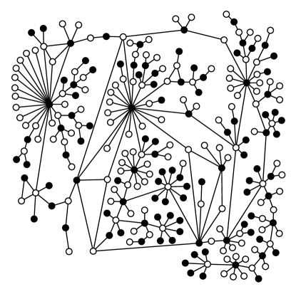
Refer to caption
Figure 7: The HIV maxcut partition. The maximum cut consists of the sets of black and white vertices; the cut-set consists of the edges between the black and white vertices.

Next, we consider a confidence set of β𝛽\beta, assuming that the HIV graph is the true graph. We apply the two-statistic test of Algorithm 9 with the same algorithm parameters. The resulting p𝑝p-values are plotted as a function of β𝛽\beta in Figure 8.

Refer to caption
Figure 8: The p𝑝p-values as a function of β𝛽\beta for the HIV graph using the two-statistic test. The two statistics are W𝑊W and W𝑊-W, i.e., the p𝑝p-value is small if W𝑊W is either too big or too small. Values of β𝛽\beta above the horizontal line at 0.050.050.05 are in the 0.80.80.8-confidence set.

If we consider a confidence interval formed by the smallest and largest values of β𝛽\beta for which the p𝑝p-value is greater than 0.050.050.05, i.e., ignoring fluctuations around 0.050.050.05, the resulting interval is [1.14,10]1.1410[1.14,10]. Thus, we have evidence for spreading on the HIV graph for β𝛽\beta in this interval.

Appendix D Simulations

This section reports the results of additional simulations we performed to validate our permutation test. Our main interest was to explore the power of our test on various graphs. We compared the algorithms proposed in [39], computed with respect to the following test statistics:

  1. 1.

    The infection radius R()𝑅R(\mathcal{I}), defined by

    R𝒢():=minv𝒱{maxud𝒢(u,v)},assignsubscript𝑅𝒢subscript𝑣𝒱subscript𝑢subscript𝑑𝒢𝑢𝑣R_{\mathcal{G}}(\mathcal{I}):=\min_{v\in\mathcal{V}}\left\{\max_{u\in\mathcal{I}}d_{\mathcal{G}}(u,v)\right\},

    where d𝒢(u,v)subscript𝑑𝒢𝑢𝑣d_{\mathcal{G}}(u,v) is the length of the shortest path connecting u𝑢u to v𝑣v in 𝒢𝒢\mathcal{G}.

  2. 2.

    The Steiner minimal tree, defined for a subset of vertices M𝑀M in a connected graph 𝒢𝒢\mathcal{G} to be a subtree of minimal edge weight containing all vertices in M𝑀M [21]. Here, M𝑀M is the set of infected vertices and each edge has unit weight.

    We are interested in a hypothesis test computed with respect to the edge weight of the Steiner minimal tree. However, finding the Steiner minimal tree is NP-complete [20], so the statistic used for simulations is based on an approximate Steiner minimal tree, computed via a tractable algorithm due to [38]. Let T()𝑇T(\mathcal{I}) be the edge weight of the approximate Steiner minimal tree.

The algorithms of [39] reject the null hypothesis if the statistic R()𝑅R(\mathcal{I}) or T()𝑇T(\mathcal{I}), evaluated on 𝒢1subscript𝒢1\mathcal{G}_{1}, exceeds a certain threshold. The corresponding tests are called the Threshold Ball (TB) and Threshold Tree (TT) algorithms. The threshold for the TB algorithm is computed theoretically to be 1.1d2(knlog(logn)/(nc))1d1.1superscript𝑑2superscript𝑘𝑛𝑛𝑛𝑐1𝑑1.1d^{2}\left(kn\log(\log n)/(n-c)\right)^{\frac{1}{d}}, when 𝒢1subscript𝒢1\mathcal{G}_{1} is a toroidal grid of dimension d𝑑d. For non-toroidal graphs, no threshold is provided, so our approach was to try to select a value of d𝑑d appropriate to the threshold calculation. In the case of the TT algorithm, the threshold suggested by [39] is kn(loglogn)3/(nc)𝑘𝑛superscript𝑛3𝑛𝑐kn(\log\log n)^{3}/(n-c).

Note that both R𝑅R and T𝑇T are defined in relation to the topology of 𝒢1subscript𝒢1\mathcal{G}_{1}, so they are Π1subscriptΠ1\Pi_{1}-invariant. Thus, we may apply Algorithm 2 and compare the results of the permutation test directly to the thresholding algorithms proposed by [39]. We write 𝒜2(S,B,α)subscript𝒜2𝑆𝐵𝛼\mathcal{A}_{2}(S,B,\alpha) to denote the result of applying Algorithm 2 with Π1subscriptΠ1\Pi_{1}-invariant statistic S𝑆S, based on B𝐵B randomly drawn permutations, with Type I error level α𝛼\alpha. We write 𝒜TB(d)subscript𝒜𝑇𝐵𝑑\mathcal{A}_{TB}(d) and 𝒜TTsubscript𝒜𝑇𝑇\mathcal{A}_{TT} to denote the TB algorithm with parameter d𝑑d and the TT algorithms, respectively.

D.1 Vertex-transitive graphs

For the first set of simulations, we let 𝒢0subscript𝒢0\mathcal{G}_{0} be the empty graph and 𝒢1subscript𝒢1\mathcal{G}_{1} the 2-dimensional toroidal grid on n𝑛n vertices. We set n{2500,10000}𝑛250010000n\in\{2500,10000\} and k=c=500𝑘𝑐500k=c=500. The results are based on 1000 simulations, for λ=1𝜆1\lambda=1 and β{1,10,100,1000}𝛽1101001000\beta\in\{1,10,100,1000\}. Table 1 contains the numerical results.

Algorithm 2 with the edges-within statistic W𝑊W performed significantly better than all other algorithms in terms of Type II error. Note that the Type II error for Algorithm 2 with statistics R𝑅R and T𝑇T decreases as β𝛽\beta increases. On the other hand, the TB and TT algorithms are uninformative for both grid sizes, since the thresholds set by the algorithms result in a rejection rule that never rejects the null hypothesis. This emphasizes an important feature of our permutation test, which always provides Type I error control, in contrast to the methods of [39], which only guarantee that the Type I error will converge to 0 as n𝑛n grows. Further note that our simulations involve a parameter λ>0𝜆0\lambda>0, which is not covered by the theory of [39]. On the other hand, for large β𝛽\beta, most infected nodes should contract the disease from a neighbor rather than exogenous sources.

Size Algorithm Threshold Type I Error Type II Error by β𝛽\beta
111 101010 100100100 100010001000
n=2,500𝑛2500n=2,500 𝒜2(W, 100, 0.01)subscript𝒜2𝑊1000.01\mathcal{A}_{2}(W,\;100,\;0.01) 220220220 0.0280.0280.028 0.0000.0000.000 0.0000.0000.000 0.0000.0000.000 0.0000.0000.000
𝒜2(R, 100, 0.01)subscript𝒜2𝑅1000.01\mathcal{A}_{2}(R,\;100,\;0.01) 454545 0.1500.1500.150 0.5170.5170.517 0.0000.0000.000 0.0000.0000.000 0.0000.0000.000
𝒜2(T, 100, 0.01)subscript𝒜2𝑇1000.01\mathcal{A}_{2}(T,\;100,\;0.01) 118611861186 0.0090.0090.009 0.8580.8580.858 0.0500.0500.050 0.0000.0000.000 0.0000.0000.000
𝒜TB(2)subscript𝒜𝑇𝐵2\mathcal{A}_{TB}(2) 157157157 1.0001.0001.000 0.0000.0000.000 0.0000.0000.000 0.0000.0000.000 0.0000.0000.000
𝒜TTsubscript𝒜𝑇𝑇\mathcal{A}_{TT} 544154415441 1.0001.0001.000 0.0000.0000.000 0.0000.0000.000 0.0000.0000.000 0.0000.0000.000
n=10,000𝑛10000n=10,000 𝒜2(W, 100, 0.01)subscript𝒜2𝑊1000.01\mathcal{A}_{2}(W,\;100,\;0.01) 636363 0.0260.0260.026 0.0000.0000.000 0.0000.0000.000 0.0000.0000.000 0.0000.0000.000
𝒜2(R, 100, 0.01)subscript𝒜2𝑅1000.01\mathcal{A}_{2}(R,\;100,\;0.01) 878787 0.0010.0010.001 1.0001.0001.000 0.9150.9150.915 0.0000.0000.000 0.0000.0000.000
𝒜2(T, 100, 0.01)subscript𝒜2𝑇1000.01\mathcal{A}_{2}(T,\;100,\;0.01) 2,50925092,509 0.0080.0080.008 0.9700.9700.970 0.2060.2060.206 0.0000.0000.000 0.0000.0000.000
𝒜TB(2)subscript𝒜𝑇𝐵2\mathcal{A}_{TB}(2) 150150150 1.0001.0001.000 0.0000.0000.000 0.0000.0000.000 0.0000.0000.000 0.0000.0000.000
𝒜TTsubscript𝒜𝑇𝑇\mathcal{A}_{TT} 5,76057605,760 1.0001.0001.000 0.0000.0000.000 0.0000.0000.000 0.0000.0000.000 0.0000.0000.000
Table 1: Threshold, Type I error, and Type II error for algorithms on the two-dimensional toroidal grid graph of size n𝑛n. Here, 𝒢0subscript𝒢0\mathcal{G}_{0} is the empty graph. We set k=c=500𝑘𝑐500k=c=500. The statistic W𝑊W performs best by far, and the permutation tests offer more reasonable error bounds. The Type I and Type II errors are approximated using 100010001000 simulations each.

D.2 Online social network

In order to gauge the performance of our algorithm on more “irregular” networks, we performed simulations on real social network graphs with the empty graph as the null. We used two connected components of the Facebook social network from the Stanford Network Analysis Project (SNAP) [34]. The graphs, which we refer to as Facebook 1 and Facebook 2, correspond to users who downloaded the Social Circles app and can be seen in Figure 9.
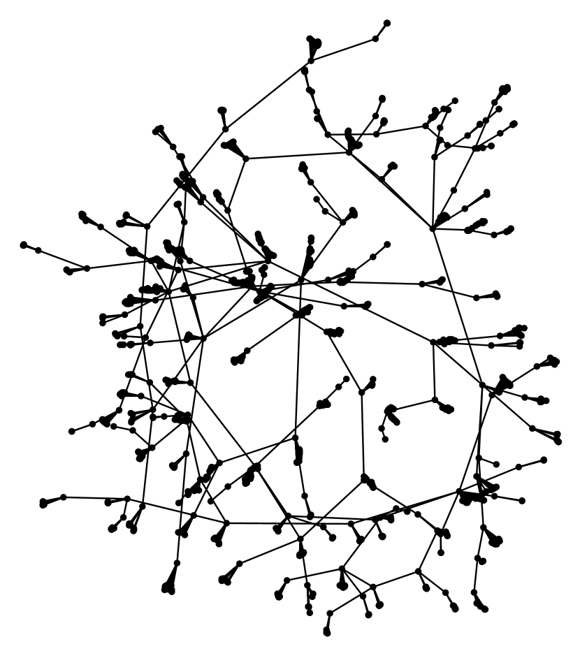
Refer to caption
Refer to caption
Figure 9: The Facebook 1 and Facebook 2 graphs, with 204020402040 and 156715671567 nodes. Note that the graphs contain a large proportion of leaves.

We simulated 1000 infections on the graphs with k=200𝑘200k=200, c=300𝑐300c=300, λ=1𝜆1\lambda=1, and β{1,10,100,1000}𝛽1101001000\beta\in\{1,10,100,1000\}. For the TB algorithm, we chose the integer d𝑑d providing the smallest threshold. Table 2 details the results. As seen in the table, Algorithm 2 with statistic W𝑊W again performed better than the other algorithms in terms of Type II error. The TB and TT algorithms performed poorly, since the thresholds for all values of d𝑑d are too large.

Network Algorithm Threshold Type I Error Type II Error by β𝛽\beta
111 101010 100100100 100010001000
Facebook 1 𝒜2(W, 200, 0.01)subscript𝒜2𝑊2000.01\mathcal{A}_{2}(W,\;200,\;0.01) 464646 0.0050.0050.005 0.2420.2420.242 0.0000.0000.000 0.0000.0000.000 0.0000.0000.000
𝒜2(R, 200, 0.01)subscript𝒜2𝑅2000.01\mathcal{A}_{2}(R,\;200,\;0.01) 111111 0.0180.0180.018 0.9580.9580.958 0.7980.7980.798 0.3070.3070.307 0.0620.0620.062
𝒜2(T, 200, 0.01)subscript𝒜2𝑇2000.01\mathcal{A}_{2}(T,\;200,\;0.01) 273273273 0.0040.0040.004 0.7000.7000.700 0.0000.0000.000 0.0000.0000.000 0.0000.0000.000
𝒜TB(3)subscript𝒜𝑇𝐵3\mathcal{A}_{TB}(3) 777777 1.0001.0001.000 0.0000.0000.000 0.0000.0000.000 0.0000.0000.000 0.0000.0000.000
𝒜TTsubscript𝒜𝑇𝑇\mathcal{A}_{TT} 196419641964 1.0001.0001.000 0.0000.0000.000 0.0000.0000.000 0.0000.0000.000 0.0000.0000.000
Facebook 2 𝒜2(W, 100, 0.01)subscript𝒜2𝑊1000.01\mathcal{A}_{2}(W,\;100,\;0.01) 515151 0.0170.0170.017 0.0480.0480.048 0.0000.0000.000 0.0000.0000.000 0.0010.0010.001
𝒜2(R, 100, 0.01)subscript𝒜2𝑅1000.01\mathcal{A}_{2}(R,\;100,\;0.01) 101010 0.0070.0070.007 0.9870.9870.987 0.8300.8300.830 0.3390.3390.339 0.0910.0910.091
𝒜2(T, 100, 0.01)subscript𝒜2𝑇1000.01\mathcal{A}_{2}(T,\;100,\;0.01) 249249249 0.0290.0290.029 0.2900.2900.290 0.0000.0000.000 0.0000.0000.000 0.0000.0000.000
𝒜TB(3)subscript𝒜𝑇𝐵3\mathcal{A}_{TB}(3) 787878 1.0001.0001.000 0.0000.0000.000 0.0000.0000.000 0.0000.0000.000 0.0000.0000.000
𝒜TTsubscript𝒜𝑇𝑇\mathcal{A}_{TT} 196519651965 1.0001.0001.000 0.0000.0000.000 0.0000.0000.000 0.0000.0000.000 0.0000.0000.000
Table 2: Threshold, Type I error, and Type II error for algorithms when 𝒢1subscript𝒢1\mathcal{G}_{1} is one of the subsets of the Facebook graph. Here, we set k=200𝑘200k=200 and c=300𝑐300c=300. Note that 𝒜2(W,B,α)subscript𝒜2𝑊𝐵𝛼\mathcal{A}_{2}(W,B,\alpha) seems to perform better than the other algorithms.

D.3 Erdős-Renyi versus stochastic block model graphs
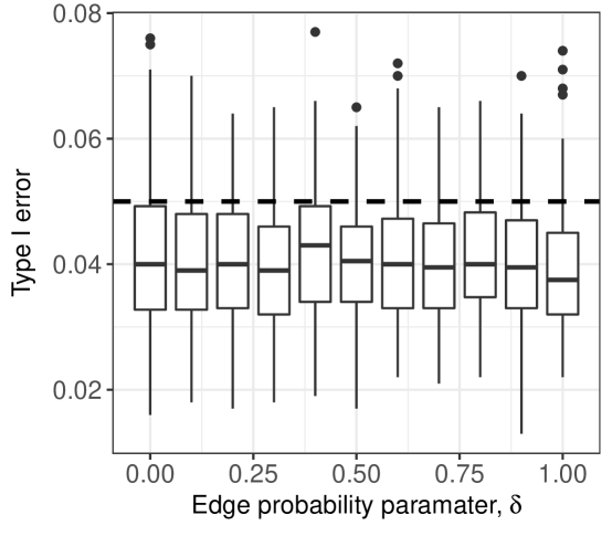
Refer to caption
Figure 10: The Type I error of the permutation test applied to the test of an Erdős-Renyi random graph versus a two-block stochastic block model graph on n=500𝑛500n=500 vertices and k=c=50𝑘𝑐50k=c=50. The edge density is p=log(n)/n𝑝𝑛𝑛p=\log(n)/n, and the within-block connectivity is a=2δp𝑎2𝛿𝑝a=2\delta p and β=1𝛽1\beta=1. On average, the permutation test controls the Type I error at the nominal level α=0.05𝛼0.05\alpha=0.05.

For our first set of random graph simulations, we considered an infection spreading on an Erdős-Renyi graph, versus a two-block stochastic block model with equal-sized partitions, where n=500𝑛500n=500. We let k=c=50𝑘𝑐50k=c=50. In the null graph, edges exist independently with probability p=log(n)/n𝑝𝑛𝑛p=\log(n)/n. In the alternative graph, the probability that an edge exists between nodes in the same partition is a𝑎a, and the probability that an edge exists between nodes in different partitions is b𝑏b, where a/2+b/2=p𝑎2𝑏2𝑝a/2+b/2=p. We let a=2δp𝑎2𝛿𝑝a=2\delta p and varied δ𝛿\delta in [0,1]01[0,1] in increments of 0.10.10.1. To estimate thresholds and error probabilities, we sampled each infection process 100010001000 times. We drew 100100100 pairs of random graphs for each δ𝛿\delta.

Lemma 15 predicts the validity of the permutation test in controlling Type I error. Furthermore, we expect the Type II error to decrease as the infections become sufficiently dissimilar through increasing β𝛽\beta or δ𝛿\delta. The first of these conclusions is verified by examining Figure 10: As δ𝛿\delta varies, the permutation test controls the Type I error at a level α=0.05𝛼0.05\alpha=0.05 on average, and with reasonably high probability. Furthermore, even outliers had Type I errors of no more than 0.080.080.08.

Refer to caption
Figure 11: The Type II error of the permutation test applied to the test of an Erdős-Renyi random graph versus a two-block stochastic block model graph on n=500𝑛500n=500 vertices and k=c=50𝑘𝑐50k=c=50. The edge density is p=log(n)/n𝑝𝑛𝑛p=\log(n)/n, and the within-block connectivity is a=2δp𝑎2𝛿𝑝a=2\delta p. The markers denote the average error, and the bars denote the range over the 100100100 simulated graphs. Perhaps surprisingly, the Type II error does not seem to depend on δ𝛿\delta. However, the Type II error decreases with β1subscript𝛽1\beta_{1}.
Refer to caption
Figure 12: The Type II error simulating the distribution of \mathcal{I} on an Erdős-Renyi 𝒢0subscript𝒢0\mathcal{G}_{0} with parameters β0=n=500subscript𝛽0𝑛500\beta_{0}=n=500 against a two-block stochastic block model 𝒢1subscript𝒢1\mathcal{G}_{1}. Here, a=2δp𝑎2𝛿𝑝a=2\delta p and b=2pa𝑏2𝑝𝑎b=2p-a are the within- and between-block edge probabilities. Additionally, we set k=c=50𝑘𝑐50k=c=50. The marker indicates the average value across 100100100 graph realizations, and the bars show the range of Type II errors. Perhaps surprisingly, this graph is very similar to Figure 11, both in terms of the average Type II error and range of values.

To examine the Type II error, we provide two plots. First, Figure 11 shows the average Type II error for various levels of β1subscript𝛽1\beta_{1} and δ𝛿\delta, when β0=0subscript𝛽00\beta_{0}=0. The marker indicates the average value across the 100100100 graph realizations, and the bars show the range of Type II errors. Additionally, the bars near each point indicate the range of the Type II errors across simulated graphs. Note that the Type II error is low for even modest values of β1subscript𝛽1\beta_{1}. The second plot is Figure 12. Here, the mean Type II error is plotted for various levels of β1subscript𝛽1\beta_{1} and δ𝛿\delta, where β0=nsubscript𝛽0𝑛\beta_{0}=n. Additionally, the bars near each point indicate the range of Type II errors over simulated graphs. Note that Figures 11 and 12 are very similar. Thus, even strong spreading on the Erdős-Renyi random graph does not seem to affect Type II error both in terms of the average and the range of values.

D.4 Correlated Erdős-Renyi random graphs

We now consider a case where the permutation test performs poorly, by examining correlated Erdős-Renyi random graphs. We took 𝒢0subscript𝒢0\mathcal{G}_{0} to be an Erdős-Renyi graph on n=500𝑛500n=500 nodes, with p=log(n)/n𝑝𝑛𝑛p=\log(n)/n. We set the infection parameters to be k=c=50𝑘𝑐50k=c=50. The alternative graph 𝒢1subscript𝒢1\mathcal{G}_{1} was also an Erdős-Renyi random graph, with edges drawn independently with probability p𝑝p. However, the existence of an edge (u,v)𝑢𝑣(u,v) in 𝒢0subscript𝒢0\mathcal{G}_{0} and 𝒢1subscript𝒢1\mathcal{G}_{1} was correlated, so γp𝛾𝑝\gamma p was the probability of (u,v)𝑢𝑣(u,v) existing in both graphs, where γ𝛾\gamma in [0,1]01[0,1] was taken in increments of 0.10.10.1. Note that γ=p𝛾𝑝\gamma=p corresponds to independent draws. To estimate thresholds and error probabilities for each graph, we sampled infection processes 100010001000 times for each set of parameters. Finally, we drew 100100100 pairs of graphs (𝒢0,𝒢1)subscript𝒢0subscript𝒢1(\mathcal{G}_{0},\mathcal{G}_{1}).

Due to correlations in edge appearance probabilities in 𝒢0subscript𝒢0\mathcal{G}_{0} and 𝒢1subscript𝒢1\mathcal{G}_{1}, our theory for permutation testing no longer applies. Intuitively, we expect that as γ𝛾\gamma increases, the test loses its Type I error control: For larger values of γ𝛾\gamma, the edges of 𝒢0subscript𝒢0\mathcal{G}_{0} and 𝒢1subscript𝒢1\mathcal{G}_{1} are more positively correlated, which increases the probability that the vertices of an edge (u,v)𝑢𝑣(u,v) in 1subscript1\mathcal{E}_{1} are infected under the null distribution. Thus, the permutation test sets the threshold for the test using W1subscript𝑊1W_{1} to be too low, causing a large Type I error. Indeed, this behavior is seen in Figure 13, where we see that the nominal Type I error level α=0.05𝛼0.05\alpha=0.05 is far from achieved for every realization with γ0.2𝛾0.2\gamma\geq 0.2.

Refer to caption
Figure 13: The Type I error of the permutation test applied to correlated Erdős-Renyi random graphs on n=500𝑛500n=500 vertices. The marginal probability of an edge (u,v)𝑢𝑣(u,v) is p=log(n)/n𝑝𝑛𝑛p=\log(n)/n in both the null and alternative, and the probability of the edge in both graphs is γp𝛾𝑝\gamma p. As γ𝛾\gamma increases, the edge correlation increases, causing the Type I error to increase. Here, β=1𝛽1\beta=1 and k=c=50𝑘𝑐50k=c=50.
Refer to caption
Figure 14: The Type II error of the permutation test applied to correlated Erdős-Renyi random graphs on n=500𝑛500n=500 vertices. The marginal probability of an edge (u,v)𝑢𝑣(u,v) is p=log(n)/n𝑝𝑛𝑛p=\log(n)/n in both the null and alternative, and the probability of the edge in both graphs is γp𝛾𝑝\gamma p. The marker indicates the average Type II error, and the bars indicate the range. Perhaps surprisingly, Figure 14 resembles Figures 11 and 12, despite the difference in graph structures.

The behavior of the Type II error is more nuanced in this case. In particular, for high values of γ𝛾\gamma, we would still expect the Type II error to be roughly on the same order as in the case of the stochastic block model. However, if we were to set the threshold using the actual null distribution, meaning the correlated random graph 𝒢0subscript𝒢0\mathcal{G}_{0}, perhaps the threshold would be sufficiently elevated by the correlated edges, which would in turn increase the Type II error. We do indeed see these behaviors in Figures 14 and 15. In the first figure, the Type II error does not depend on γ𝛾\gamma, since 𝒢1subscript𝒢1\mathcal{G}_{1} is always an Erdős-Renyi random graph with parameter p𝑝p. In the second figure, we see that the Type II error increases drastically when considering a threshold set by simulating on 𝒢0subscript𝒢0\mathcal{G}_{0}. However, note that for large values of β1subscript𝛽1\beta_{1}, the graphs can still be distinguished even with moderately large correlation. This provides hope that in correlated cases, infection patterns that depend very strongly on the graph topology could still yield correct inference for the true graph.
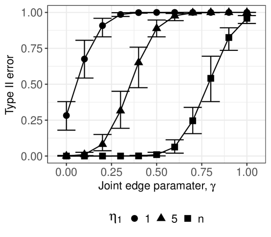
Refer to caption
Figure 15: The Type II error between a pair of correlated Erdős-Renyi random graphs 𝒢0subscript𝒢0\mathcal{G}_{0} and 𝒢1subscript𝒢1\mathcal{G}_{1} when β0=n=500subscript𝛽0𝑛500\beta_{0}=n=500. The marginal probability of an edge (u,v)𝑢𝑣(u,v) in either graph is p=log(n)/n𝑝𝑛𝑛p=\log(n)/n, and the probability of the edge in both graphs is γp𝛾𝑝\gamma p. Additionally, we set k=c=50𝑘𝑐50k=c=50. The markers denote the average Type II errors, and the bars denote the range. Note that this figure is very different from Figure 14. In particular, for higher values of γ𝛾\gamma, the Type II error is much worse, since the graphs become similar. However, note that if β1subscript𝛽1\beta_{1} is sufficiently high, the graphs can still be distinguished even for moderately large γ𝛾\gamma.

Appendix E Proofs

In this section, we provide proofs of our main results and the propositions.

E.1 Proofs of main theorems

Proof of Theorem 1.

Note that under H0subscript𝐻0H_{0}, and for any set \mathcal{B}, we have

0()=0(π)=1|Π0|π0Π00(π0),subscript0subscript0𝜋1subscriptΠ0subscriptsubscript𝜋0subscriptΠ0subscript0subscript𝜋0\mathbb{P}_{0}\left(\mathcal{I}\in\mathcal{B}\right)=\mathbb{P}_{0}\left(\pi\mathcal{I}\in\mathcal{B}\right)=\frac{1}{|\Pi_{0}|}\sum_{\pi_{0}\in\Pi_{0}}\mathbb{P}_{0}\left(\pi_{0}\mathcal{I}\in\mathcal{B}\right),

where the first equality is by assumption and the second is by averaging. The first equality is proven in detail for our models in Section E.2. In particular,

0(S()t)subscript0𝑆𝑡\displaystyle\mathbb{P}_{0}\left(S(\mathcal{I})\leq t\right) =0(S1(,t])absentsubscript0superscript𝑆1𝑡\displaystyle=\mathbb{P}_{0}\left(\mathcal{I}\in S^{-1}(-\infty,t]\right)
=1|Π0|π0Π00(π0S1(,t])absent1subscriptΠ0subscriptsubscript𝜋0subscriptΠ0subscript0subscript𝜋0superscript𝑆1𝑡\displaystyle=\frac{1}{|\Pi_{0}|}\sum_{\pi_{0}\in\Pi_{0}}\mathbb{P}_{0}\left(\pi_{0}\mathcal{I}\in S^{-1}(-\infty,t]\right)
=1|Π0|π0Π00(S(π0)t).absent1subscriptΠ0subscriptsubscript𝜋0subscriptΠ0subscript0𝑆subscript𝜋0𝑡\displaystyle=\frac{1}{|\Pi_{0}|}\sum_{\pi_{0}\in\Pi_{0}}\mathbb{P}_{0}\left(S(\pi_{0}\mathcal{I})\leq t\right).

Now let {g1,,gm}subscript𝑔1subscript𝑔𝑚\{g_{1},\dots,g_{m}\} denote coset representatives for Π0subscriptΠ0\Pi_{0} in the permutation group Snsubscript𝑆𝑛S_{n}, so {g1Π0,,gmΠ0}subscript𝑔1subscriptΠ0subscript𝑔𝑚subscriptΠ0\{g_{1}\Pi_{0},\dots,g_{m}\Pi_{0}\} partitions Snsubscript𝑆𝑛S_{n} and has cardinality

m=|Sn||Π0|=n!|Π0|.𝑚subscript𝑆𝑛subscriptΠ0𝑛subscriptΠ0m=\frac{|S_{n}|}{|\Pi_{0}|}=\frac{n!}{|\Pi_{0}|}.

By assumption, we may choose giΠ1subscript𝑔𝑖subscriptΠ1g_{i}\in\Pi_{1} for each 1im1𝑖𝑚1\leq i\leq m. Since S𝑆S is a Π1subscriptΠ1\Pi_{1}-invariant statistic, this means S(giπ0)=S(π0)𝑆subscript𝑔𝑖subscript𝜋0𝑆subscript𝜋0S(g_{i}\pi_{0}\mathcal{I})=S(\pi_{0}\mathcal{I}) for each i𝑖i. Hence,

0(S()t)=1|Π0|π0Π01m1im0(S(giπ0)t)=1n!πSn0(S(π)t),subscript0𝑆𝑡1subscriptΠ0subscriptsubscript𝜋0subscriptΠ01𝑚subscript1𝑖𝑚subscript0𝑆subscript𝑔𝑖subscript𝜋0𝑡1𝑛subscript𝜋subscript𝑆𝑛subscript0𝑆𝜋𝑡\displaystyle\mathbb{P}_{0}\left(S(\mathcal{I})\leq t\right)=\frac{1}{|\Pi_{0}|}\sum_{\pi_{0}\in\Pi_{0}}\frac{1}{m}\sum_{1\leq i\leq m}\mathbb{P}_{0}\left(S(g_{i}\pi_{0}\mathcal{I})\leq t\right)=\frac{1}{n!}\sum_{\pi\in S_{n}}\mathbb{P}_{0}\left(S(\pi\mathcal{I})\leq t\right),

implying that S()𝑆S(\mathcal{I}) and S(π)𝑆𝜋S(\pi\mathcal{I}) have the same distribution when πUniform(Sn)similar-to𝜋Uniformsubscript𝑆𝑛\pi\sim\text{Uniform}(S_{n}). ∎

Proof of Theorem 2.

By Theorem 1, we have

0(S()t)=1n!πSn0(S(π)t),subscript0𝑆𝑡1𝑛subscript𝜋subscript𝑆𝑛subscript0𝑆𝜋𝑡\mathbb{P}_{0}\left(S(\mathcal{I})\leq t\right)=\frac{1}{n!}\sum_{\pi\in S_{n}}\mathbb{P}_{0}\left(S(\pi\mathcal{I})\leq t\right),

for each t𝑡t\in\mathbb{R}. Conditioning on the infection vector \mathcal{I}, we obtain

0(S()t)subscript0𝑆𝑡\displaystyle\mathbb{P}_{0}\left(S(\mathcal{I})\leq t\right) =𝕀k,c0()1n!πSn0(S(π)t|)absentsubscriptsubscript𝕀𝑘𝑐subscript01𝑛subscript𝜋subscript𝑆𝑛subscript0𝑆𝜋conditional𝑡\displaystyle=\sum_{\mathcal{I}\in\mathbb{I}_{k,c}}\mathbb{P}_{0}\left(\mathcal{I}\right)\frac{1}{n!}\sum_{\pi\in S_{n}}\mathbb{P}_{0}\left(S(\pi\mathcal{I})\leq t\;\Big{|}\;\mathcal{I}\right)
=1n!𝕀k,cπSn0()0(S(π)t|).absent1𝑛subscriptsubscript𝕀𝑘𝑐subscript𝜋subscript𝑆𝑛subscript0subscript0𝑆𝜋conditional𝑡\displaystyle=\frac{1}{n!}\sum_{\mathcal{I}\in\mathbb{I}_{k,c}}\sum_{\pi\in S_{n}}\mathbb{P}_{0}\left(\mathcal{I}\right)\mathbb{P}_{0}\left(S(\pi\mathcal{I})\leq t\;\Big{|}\;\mathcal{I}\right).

Fix some J𝕀k,c𝐽subscript𝕀𝑘𝑐J\in\mathbb{I}_{k,c}. For an infection \mathcal{I}, let πJ,subscript𝜋𝐽\pi_{J,\mathcal{I}} be a permutation mapping \mathcal{I} to J𝐽J. Then =πJ,1Jsuperscriptsubscript𝜋𝐽1𝐽\mathcal{I}=\pi_{J,\mathcal{I}}^{-1}J, so π=ππJ,1J𝜋𝜋superscriptsubscript𝜋𝐽1𝐽\pi\mathcal{I}=\pi\pi_{J,\mathcal{I}}^{-1}J, and

0(S()t)subscript0𝑆𝑡\displaystyle\mathbb{P}_{0}\left(S(\mathcal{I})\leq t\right) =1n!𝕀k,cπSn0()0(S(ππJ,1J)t|)absent1𝑛subscriptsubscript𝕀𝑘𝑐subscript𝜋subscript𝑆𝑛subscript0subscript0𝑆𝜋superscriptsubscript𝜋𝐽1𝐽conditional𝑡\displaystyle=\frac{1}{n!}\sum_{\mathcal{I}\in\mathbb{I}_{k,c}}\sum_{\pi\in S_{n}}\mathbb{P}_{0}\left(\mathcal{I}\right)\mathbb{P}_{0}\left(S\left(\pi\pi_{J,\mathcal{I}}^{-1}J\right)\leq t\;\Big{|}\;\mathcal{I}\right)
=1n!𝕀k,c0()πSn0(S(πJ)t|)absent1𝑛subscriptsubscript𝕀𝑘𝑐subscript0subscriptsuperscript𝜋subscript𝑆𝑛subscript0𝑆superscript𝜋𝐽conditional𝑡\displaystyle=\frac{1}{n!}\sum_{\mathcal{I}\in\mathbb{I}_{k,c}}\mathbb{P}_{0}\left(\mathcal{I}\right)\sum_{\pi^{\prime}\in S_{n}}\mathbb{P}_{0}\left(S(\pi^{\prime}J)\leq t\;\Big{|}\;\mathcal{I}\right)
=1n!𝕀k,c0()πSn0(S(πJ)t),absent1𝑛subscriptsubscript𝕀𝑘𝑐subscript0subscriptsuperscript𝜋subscript𝑆𝑛subscript0𝑆superscript𝜋𝐽𝑡\displaystyle=\frac{1}{n!}\sum_{\mathcal{I}\in\mathbb{I}_{k,c}}\mathbb{P}_{0}\left(\mathcal{I}\right)\sum_{\pi^{\prime}\in S_{n}}\mathbb{P}_{0}\left(S(\pi^{\prime}J)\leq t\right),

where we denote π=ππJ,1superscript𝜋𝜋superscriptsubscript𝜋𝐽1\pi^{\prime}=\pi\pi_{J,\mathcal{I}}^{-1}. In the last step, the conditioning on \mathcal{I} becomes irrelevant because we sum over all permutations in Snsubscript𝑆𝑛S_{n}. Note that

0(S(πJ)t)=𝟏{S(πJ)t},subscript0𝑆superscript𝜋𝐽𝑡1𝑆superscript𝜋𝐽𝑡\mathbb{P}_{0}(S(\pi^{\prime}J)\leq t)=\mathbf{1}\left\{S(\pi^{\prime}J)\leq t\right\},

since all quantities are deterministic. Hence,

0(S()t)subscript0𝑆𝑡\displaystyle\mathbb{P}_{0}\left(S(\mathcal{I})\leq t\right) =1n!𝕀k,c0()πSn𝟏{S(πJ)t}=1n!πSn𝟏{S(πJ)t}.absent1𝑛subscriptsubscript𝕀𝑘𝑐subscript0subscriptsuperscript𝜋subscript𝑆𝑛1𝑆superscript𝜋𝐽𝑡1𝑛subscriptsuperscript𝜋subscript𝑆𝑛1𝑆superscript𝜋𝐽𝑡\displaystyle=\frac{1}{n!}\sum_{\mathcal{I}\in\mathbb{I}_{k,c}}\mathbb{P}_{0}\left(\mathcal{I}\right)\sum_{\pi^{\prime}\in S_{n}}\mathbf{1}\left\{S(\pi^{\prime}J)\leq t\right\}=\frac{1}{n!}\sum_{\pi^{\prime}\in S_{n}}\mathbf{1}\left\{S(\pi^{\prime}J)\leq t\right\}.

This justifies the permutation test described in Algorithm 1: The threshold tαsubscript𝑡𝛼t_{\alpha} to bound the Type I error at level α𝛼\alpha may be computed explicitly from computing the appropriate quantile of S𝑆S with respect to all n!𝑛n! permutations of J𝐽J. ∎

Proof of Theorem 7.

Let 𝒪Π1(1)subscript𝒪subscriptΠ11\mathcal{O}_{\Pi_{1}}(1) denote the orbit of vertex 1 in Π1=Aut(G1)subscriptΠ1Autsubscript𝐺1\Pi_{1}=\operatorname{Aut}(G_{1}), and note that by assumption, |𝒪Π1(1)|<nsubscript𝒪subscriptΠ11𝑛|\mathcal{O}_{\Pi_{1}}(1)|<n. Consider the statistic

S(J)=v𝒪Π1(1)1{Jv=1},𝑆𝐽subscript𝑣subscript𝒪subscriptΠ111subscript𝐽𝑣1S(J)=\sum_{v\in\mathcal{O}_{\Pi_{1}}(1)}1\{J_{v}=1\},

which counts the number of infected vertices in 𝒪Π1(1)subscript𝒪subscriptΠ11\mathcal{O}_{\Pi_{1}}(1). Note that S𝑆S is clearly Π1subscriptΠ1\Pi_{1}-invariant. We claim that S()𝑆S(\mathcal{I}) and S(π)𝑆𝜋S(\pi\mathcal{I}) do not have the same distribution under H0subscript𝐻0H_{0}, when πUniform(Sn)similar-to𝜋Uniformsubscript𝑆𝑛\pi\sim\text{Uniform}(S_{n}).

Let G={g1,,ga}Π0𝐺subscript𝑔1subscript𝑔𝑎subscriptΠ0G=\{g_{1},\dots,g_{a}\}\subseteq\Pi_{0} be a set consisting of coset representatives such that {Π1g1,,Π1ga}subscriptΠ1subscript𝑔1subscriptΠ1subscript𝑔𝑎\{\Pi_{1}g_{1},\dots,\Pi_{1}g_{a}\} is a partition of Π1Π0subscriptΠ1subscriptΠ0\Pi_{1}\Pi_{0}, and let H={h1,,hb}Sn\Π0𝐻subscript1subscript𝑏\subscript𝑆𝑛subscriptΠ0H=\{h_{1},\dots,h_{b}\}\subseteq S_{n}\backslash\Pi_{0} be representatives of the remaining cosets of Π1subscriptΠ1\Pi_{1} in Snsubscript𝑆𝑛S_{n}. For any observation vector J𝐽J, we have

0(S(π)=S(J))subscript0𝑆𝜋𝑆𝐽\displaystyle\mathbb{P}_{0}\left(S(\pi\mathcal{I})=S(J)\right) =1n!π1Π1gGH0(S(π1g)=S(J))absent1𝑛subscriptsubscript𝜋1subscriptΠ1subscript𝑔𝐺𝐻subscript0𝑆subscript𝜋1𝑔𝑆𝐽\displaystyle=\frac{1}{n!}\sum_{\pi_{1}\in\Pi_{1}}\sum_{g\in G\cup H}\mathbb{P}_{0}\left(S(\pi_{1}g\mathcal{I})=S(J)\right)
=|Π1|n!gGH0(S(g)=S(J))absentsubscriptΠ1𝑛subscript𝑔𝐺𝐻subscript0𝑆𝑔𝑆𝐽\displaystyle=\frac{|\Pi_{1}|}{n!}\sum_{g\in G\cup H}\mathbb{P}_{0}\left(S(g\mathcal{I})=S(J)\right)
=1a+bgGH0(S(g)=S(J)),absent1𝑎𝑏subscript𝑔𝐺𝐻subscript0𝑆𝑔𝑆𝐽\displaystyle=\frac{1}{a+b}\sum_{g\in G\cup H}\mathbb{P}_{0}\left(S(g\mathcal{I})=S(J)\right),

where the first equality uses the fact that {Π1g1,,Π1ga}{Π1h1,,Πhb}subscriptΠ1subscript𝑔1subscriptΠ1subscript𝑔𝑎subscriptΠ1subscript1Πsubscript𝑏\{\Pi_{1}g_{1},\dots,\Pi_{1}g_{a}\}\cup\{\Pi_{1}h_{1},\dots,\Pi h_{b}\} is a partition of Snsubscript𝑆𝑛S_{n}, and the second equality uses the fact that S𝑆S is Π1subscriptΠ1\Pi_{1}-invariant.

By symmetry of the spreading process on 𝒢0subscript𝒢0\mathcal{G}_{0}, we have

0(S(g)=S(J))=0(S()=S(J)),gG.formulae-sequencesubscript0𝑆𝑔𝑆𝐽subscript0𝑆𝑆𝐽for-all𝑔𝐺\mathbb{P}_{0}\left(S(g\mathcal{I})=S(J)\right)=\mathbb{P}_{0}\left(S(\mathcal{I})=S(J)\right),\qquad\forall g\in G.

Hence,

0(S(π)=S(J))=aa+b0(S()=S(J))+1a+bhH0(S(h)=S(J)).subscript0𝑆𝜋𝑆𝐽𝑎𝑎𝑏subscript0𝑆𝑆𝐽1𝑎𝑏subscript𝐻subscript0𝑆𝑆𝐽\mathbb{P}_{0}\left(S(\pi\mathcal{I})=S(J)\right)=\frac{a}{a+b}\mathbb{P}_{0}\left(S(\mathcal{I})=S(J)\right)+\frac{1}{a+b}\sum_{h\in H}\mathbb{P}_{0}\left(S(h\mathcal{I})=S(J)\right).

We will demonstrate a choice of J𝐽J for which

hH0(S(h)=S(J))b0(S()=S(J)),subscript𝐻subscript0𝑆𝑆𝐽𝑏subscript0𝑆𝑆𝐽\sum_{h\in H}\mathbb{P}_{0}\left(S(h\mathcal{I})=S(J)\right)\neq b\;\mathbb{P}_{0}\left(S(\mathcal{I})=S(J)\right),

implying that

0(S(π)=S(J))0(S()=S(J)),subscript0𝑆𝜋𝑆𝐽subscript0𝑆𝑆𝐽\mathbb{P}_{0}\left(S(\pi\mathcal{I})=S(J)\right)\neq\mathbb{P}_{0}\left(S(\mathcal{I})=S(J)\right),

so S(π)𝑆𝜋S(\pi\mathcal{I}) and S()𝑆S(\mathcal{I}) cannot have the same distribution.

Let J𝕀k,c𝐽subscript𝕀𝑘𝑐J\in\mathbb{I}_{k,c} be a vector such that S(J)=m𝑆𝐽𝑚S(J)=m, for some m𝑚m to be specified later. Then 0(S()=S(J))subscript0𝑆𝑆𝐽\mathbb{P}_{0}\left(S(\mathcal{I})=S(J)\right) is the probability that exactly m𝑚m vertices in 𝒪Π1(1)subscript𝒪subscriptΠ11\mathcal{O}_{\Pi_{1}}(1) are infected. On the other hand, for a fixed gSn𝑔subscript𝑆𝑛g\in S_{n}, the quantity S(g)𝑆𝑔S(g\mathcal{I}) counts the number of infected vertices in g1(𝒪Π1(1))superscript𝑔1subscript𝒪subscriptΠ11g^{-1}\left(\mathcal{O}_{\Pi_{1}}(1)\right). Again using symmetry of the spreading process on 𝒢0subscript𝒢0\mathcal{G}_{0}, we have

0(S(g)=m)=0(S()=m),subscript0𝑆𝑔𝑚subscript0𝑆𝑚\mathbb{P}_{0}\left(S(g\mathcal{I})=m\right)=\mathbb{P}_{0}\left(S(\mathcal{I})=m\right),

whenever 1g1(𝒪Π1(1))1superscript𝑔1subscript𝒪subscriptΠ111\in g^{-1}\left(\mathcal{O}_{\Pi_{1}}(1)\right). However, when 1g1(𝒪Π1(1))1superscript𝑔1subscript𝒪subscriptΠ111\notin g^{-1}\left(\mathcal{O}_{\Pi_{1}}(1)\right), we have

0(S(g)=m)<0(S()=m),subscript0𝑆𝑔𝑚subscript0𝑆𝑚\mathbb{P}_{0}\left(S(g\mathcal{I})=m\right)<\mathbb{P}_{0}\left(S(\mathcal{I})=m\right),

for some m𝑚m, since the center of the star is more likely to be infected than any of the leaves. Finally, note that hj(1)𝒪Π1(1)subscript𝑗1subscript𝒪subscriptΠ11h_{j}(1)\notin\mathcal{O}_{\Pi_{1}}(1) for some j𝑗j. Indeed, if hi(1)𝒪Π1(1)subscript𝑖1subscript𝒪subscriptΠ11h_{i}(1)\in\mathcal{O}_{\Pi_{1}}(1) for all 1ib1𝑖𝑏1\leq i\leq b, we would have π1hi(1)𝒪Π1(1)subscript𝜋1subscript𝑖1subscript𝒪subscriptΠ11\pi_{1}h_{i}(1)\in\mathcal{O}_{\Pi_{1}}(1) for all π1Π1subscript𝜋1subscriptΠ1\pi_{1}\in\Pi_{1}, contradicting the fact that the cosets cover the entire space Snsubscript𝑆𝑛S_{n}. Thus, we have 1hj1(𝒪Π1(1))1superscriptsubscript𝑗1subscript𝒪subscriptΠ111\notin h_{j}^{-1}\left(\mathcal{O}_{\Pi_{1}}(1)\right), implying that

0(S(hj)=m)<0(S()=m),subscript0𝑆subscript𝑗𝑚subscript0𝑆𝑚\mathbb{P}_{0}(S(h_{j}\mathcal{I})=m)<\mathbb{P}_{0}(S(\mathcal{I})=m),

and in particular,

i=1b0(S(hi)=S(J))<b0(S()=S(J)).superscriptsubscript𝑖1𝑏subscript0𝑆subscript𝑖𝑆𝐽𝑏subscript0𝑆𝑆𝐽\sum_{i=1}^{b}\mathbb{P}_{0}\left(S(h_{i}\mathcal{I})=S(J)\right)<b\;\mathbb{P}_{0}\left(S(\mathcal{I})=S(J)\right).

This completes the proof. ∎

E.2 Proofs of invariances

In this appendix, we derive the following key lemma concerning permutation invariance of infection statistics under the graph automorphism group. This lemma is leveraged in the proof of Theorem 1. We first outline the proof of the lemma, and then provide the proofs of several supporting lemmas.

Lemma 2.

Let Π0=Aut(𝒢0)subscriptΠ0Autsubscript𝒢0\Pi_{0}=\operatorname{Aut}(\mathcal{G}_{0}). For any π0subscript𝜋0\pi_{0} in Π0subscriptΠ0\Pi_{0}, we have

0(=J)=0(π0=J)=1|Π0|πΠ00(π=J),subscript0𝐽subscript0subscript𝜋0𝐽1subscriptΠ0subscript𝜋subscriptΠ0subscript0𝜋𝐽\mathbb{P}_{0}(\mathcal{I}=J)=\mathbb{P}_{0}(\pi_{0}\mathcal{I}=J)=\frac{1}{|\Pi_{0}|}\sum_{\pi\in\Pi_{0}}\mathbb{P}_{0}(\pi\mathcal{I}=J),

under both the stochastic spreading and conditional Ising models.

Proof.

Note that it suffices to prove the first equality, since the second equality may be obtained by averaging over Π0subscriptΠ0\Pi_{0}. Further note that once we have proved the equality for uncensored infection vectors, the extension to censored vectors follows immediately from the additive expression for the censoring measure over all possible uncensored configurations.

We begin by focusing on the stochastic spreading model. The probability of an (uncensored) infection vector J𝐽J is

0(=J)=P𝔓(J)0(𝒫=P).subscript0𝐽absentsubscript𝑃𝔓𝐽subscript0𝒫𝑃\displaystyle\begin{aligned} \mathbb{P}_{0}(\mathcal{I}=J)&=\sum_{P\in\mathfrak{P}(J)}\mathbb{P}_{0}(\mathcal{P}=P).\end{aligned}

Thus, it suffices to prove that 0(𝒫=P)=0(π0𝒫=P)subscript0𝒫𝑃subscript0subscript𝜋0𝒫𝑃\mathbb{P}_{0}(\mathcal{P}=P)=\mathbb{P}_{0}(\pi_{0}\mathcal{P}=P), for all P𝔓(J)𝑃𝔓𝐽P\in\mathfrak{P}(J), where

π0P=π0(P1,,Pk)=(π0(P1),,π0(Pk)).subscript𝜋0𝑃subscript𝜋0subscript𝑃1subscript𝑃𝑘subscript𝜋0subscript𝑃1subscript𝜋0subscript𝑃𝑘\pi_{0}P=\pi_{0}(P_{1},\dots,P_{k})=\left(\pi_{0}(P_{1}),\ldots,\pi_{0}(P_{k})\right).

The probability of a path P𝑃P is equal to

0(𝒫=P)=t=1k1+Nt,in(P)n+1t+βNt(P).subscript0𝒫𝑃absentsuperscriptsubscriptproduct𝑡1𝑘1subscript𝑁𝑡in𝑃𝑛1𝑡𝛽subscript𝑁𝑡𝑃\displaystyle\begin{aligned} \mathbb{P}_{0}(\mathcal{P}=P)&=\prod_{t=1}^{k}\frac{1+N_{t,\text{in}}(P)}{n+1-t+\beta N_{t}(P)}.\end{aligned}

Thus, it suffices to show that Nt,in(P)subscript𝑁𝑡in𝑃N_{t,\text{in}}(P) and Nt(P)subscript𝑁𝑡𝑃N_{t}(P) are permutation-invariant. This is done in Lemma 3 below.

In the case of the Ising model, we have seen that the probability of an infection J𝐽J only depends on its Hamiltonian. Lemma 4 below shows that the Hamiltonian statistic is permutation-invariant. ∎

We now provide the proofs of the supporting lemmas to Lemma 2. Note that the following lemmas are all deterministic statements in terms of a fixed graph 𝒢𝒢\mathcal{G}, with the automorphism group Π:=Aut(𝒢)assignΠAut𝒢\Pi:=\operatorname{Aut}(\mathcal{G}); they will be applied with 𝒢=𝒢0𝒢subscript𝒢0\mathcal{G}=\mathcal{G}_{0} and 𝒢1subscript𝒢1\mathcal{G}_{1} in our arguments in the paper.

Lemma 3.

The statistics Nt,insubscript𝑁𝑡inN_{t,\text{in}} and Ntsubscript𝑁𝑡N_{t} are ΠΠ\Pi-invariant when computed on graph 𝒢𝒢\mathcal{G}.

Proof.

We have

Nt,in(P)=s=1t1𝟏{(Ps,Pt)},Nt(P)=(u,v)𝟏{exactly one of u or v is in (P1,,Pt1)}.subscript𝑁𝑡in𝑃absentsuperscriptsubscript𝑠1𝑡11subscript𝑃𝑠subscript𝑃𝑡subscript𝑁𝑡𝑃absentsubscript𝑢𝑣1exactly one of u or v is in (P1,,Pt1)\displaystyle\begin{aligned} N_{t,\text{in}}(P)&=\sum_{s=1}^{t-1}\mathbf{1}\left\{(P_{s},P_{t})\in\mathcal{E}\right\},\\ N_{t}(P)&=\sum_{(u,v)\in\mathcal{E}}\mathbf{1}\left\{\text{exactly one of $u$ or $v$ is in $(P_{1},\ldots,P_{t-1})$}\right\}.\end{aligned}

For πΠ𝜋Π\pi\in\Pi, we have

Nt,in(P)=s=1t1𝟏{(Ps,Pt)π1}=s=1t1𝟏{(π(Ps),π(Pt))}=Nt,in(πP),subscript𝑁𝑡in𝑃absentsuperscriptsubscript𝑠1𝑡11subscript𝑃𝑠subscript𝑃𝑡superscript𝜋1missing-subexpressionabsentsuperscriptsubscript𝑠1𝑡11𝜋subscript𝑃𝑠𝜋subscript𝑃𝑡missing-subexpressionabsentsubscript𝑁𝑡in𝜋𝑃\displaystyle\begin{aligned} N_{t,\text{in}}(P)&=\sum_{s=1}^{t-1}\mathbf{1}\left\{(P_{s},P_{t})\in\pi^{-1}\mathcal{E}\right\}\\ &=\sum_{s=1}^{t-1}\mathbf{1}\left\{(\pi(P_{s}),\pi(P_{t}))\in\mathcal{E}\right\}\\ &=N_{t,\text{in}}(\pi P),\end{aligned}

where we have used the definition of an automorphism and the closure of groups under inversion for the first equality. Similarly, we may write

Nt(P)=(u,v)π1𝟏{exactly one of u or v is in (P1,,Pt1)}=(u,v)𝟏{exactly one of π1(u) or π1(v) is in (P1,,Pt1)}=(u,v)𝟏{exactly one of u or v is in (π(P1),,π(Pt1))}=Nt(πP).subscript𝑁𝑡𝑃absentsubscript𝑢𝑣superscript𝜋11exactly one of u or v is in (P1,,Pt1)missing-subexpressionabsentsubscript𝑢𝑣1exactly one of π1(u) or π1(v) is in (P1,,Pt1)missing-subexpressionabsentsubscript𝑢𝑣1exactly one of u or v is in (π(P1),,π(Pt1))missing-subexpressionabsentsubscript𝑁𝑡𝜋𝑃\displaystyle\begin{aligned} N_{t}(P)&=\sum_{(u,v)\in\pi^{-1}\mathcal{E}}\mathbf{1}\left\{\text{exactly one of $u$ or $v$ is in $(P_{1},\ldots,P_{t-1})$}\right\}\\ &=\sum_{(u,v)\in\mathcal{E}}\mathbf{1}\left\{\text{exactly one of $\pi^{-1}(u)$ or $\pi^{-1}(v)$ is in $(P_{1},\ldots,P_{t-1})$}\right\}\\ &=\sum_{(u,v)\in\mathcal{E}}\mathbf{1}\left\{\text{exactly one of $u$ or $v$ is in $(\pi(P_{1}),\ldots,\pi(P_{t-1}))$}\right\}\\ &=N_{t}(\pi P).\end{aligned}

Lemma 4.

The edges-within statistic W(J)=(J)𝑊𝐽superscript𝐽W(J)=\mathcal{H}^{\prime}(J) is ΠΠ\Pi-invariant when computed on graph 𝒢𝒢\mathcal{G}.

Proof.

For πΠ𝜋Π\pi\in\Pi, we have

W(J)=(u,v)𝟏{Ju=Jv=1}=(u,v)π1𝟏{Ju=Jv=1}=(u,v)𝟏{Jπ1(u)=Jπ1(v)=1}=(u,v)𝟏{(πJ)u=(πJ)v=1}=W(πJ),𝑊𝐽absentsubscript𝑢𝑣1subscript𝐽𝑢subscript𝐽𝑣1missing-subexpressionabsentsubscript𝑢𝑣superscript𝜋11subscript𝐽𝑢subscript𝐽𝑣1missing-subexpressionabsentsubscript𝑢𝑣1subscript𝐽superscript𝜋1𝑢subscript𝐽superscript𝜋1𝑣1missing-subexpressionabsentsubscript𝑢𝑣1subscript𝜋𝐽𝑢subscript𝜋𝐽𝑣1missing-subexpressionabsent𝑊𝜋𝐽\displaystyle\begin{aligned} W(J)&=\sum_{(u,v)\in\mathcal{E}}\mathbf{1}\left\{J_{u}=J_{v}=1\right\}\\ &=\sum_{(u,v)\in\pi^{-1}\mathcal{E}}\mathbf{1}\left\{J_{u}=J_{v}=1\right\}\\ &=\sum_{(u,v)\in\mathcal{E}}\mathbf{1}\left\{J_{\pi^{-1}(u)}=J_{\pi^{-1}(v)}=1\right\}\\ &=\sum_{(u,v)\in\mathcal{E}}\mathbf{1}\left\{(\pi J)_{u}=(\pi J)_{v}=1\right\}\\ &=W(\pi J),\end{aligned}

using similar arguments to the proof of Lemma 3. ∎

E.3 Hunt-Stein

Proof of Theorem 5.

Clearly, ψsuperscript𝜓\psi^{*} is ΠΠ\Pi-invariant, since for any πΠsuperscript𝜋Π\pi^{\prime}\in\Pi, we have

ψ(π)=1|Π|πΠφ(ππ)=1|Π|ππΠπφ(ππ)=1|Π|π~Πφ(π~)=ψ().superscript𝜓superscript𝜋1Πsubscript𝜋Πsuperscript𝜑𝜋superscript𝜋1Πsubscript𝜋superscript𝜋Πsuperscript𝜋superscript𝜑𝜋superscript𝜋1Πsubscript~𝜋Πsuperscript𝜑~𝜋superscript𝜓\psi^{*}(\pi^{\prime}\mathcal{I})=\frac{1}{|\Pi|}\sum_{\pi\in\Pi}\varphi^{*}(\pi\pi^{\prime}\mathcal{I})=\frac{1}{|\Pi|}\sum_{\pi\pi^{\prime}\in\Pi\pi^{\prime}}\varphi^{*}(\pi\pi^{\prime}\mathcal{I})=\frac{1}{|\Pi|}\sum_{\tilde{\pi}\in\Pi}\varphi^{*}(\tilde{\pi}\mathcal{I})=\psi^{*}(\mathcal{I}).

We now show that ψsuperscript𝜓\psi^{*} satisfies the inequality

infπΠ𝔼πθ[φ()]𝔼θ[ψ()]supπΠ𝔼πθ[φ()],θΘ.formulae-sequencesubscriptinfimum𝜋Πsubscript𝔼𝜋𝜃delimited-[]superscript𝜑subscript𝔼𝜃delimited-[]superscript𝜓subscriptsupremum𝜋Πsubscript𝔼𝜋𝜃delimited-[]superscript𝜑for-all𝜃Θ\inf_{\pi\in\Pi}\mathbb{E}_{\pi\theta}[\varphi^{*}(\mathcal{I})]\leq\mathbb{E}_{\theta}[\psi^{*}(\mathcal{I})]\leq\sup_{\pi\in\Pi}\mathbb{E}_{\pi\theta}[\varphi^{*}(\mathcal{I})],\qquad\forall\theta\in\Theta. (18)

We may write

𝔼θ[ψ()]=𝔼θ[1|Π|πΠφ(π)]=1|Π|πΠ𝔼θ[φ(π)]=1|Π|πΠ𝔼πθ[φ()].subscript𝔼𝜃delimited-[]superscript𝜓subscript𝔼𝜃delimited-[]1Πsubscript𝜋Πsuperscript𝜑𝜋1Πsubscript𝜋Πsubscript𝔼𝜃delimited-[]superscript𝜑𝜋1Πsubscript𝜋Πsubscript𝔼𝜋𝜃delimited-[]superscript𝜑\mathbb{E}_{\theta}[\psi^{*}(\mathcal{I})]=\mathbb{E}_{\theta}\left[\frac{1}{|\Pi|}\sum_{\pi\in\Pi}\varphi^{*}(\pi\mathcal{I})\right]=\frac{1}{|\Pi|}\sum_{\pi\in\Pi}\mathbb{E}_{\theta}[\varphi^{*}(\pi\mathcal{I})]=\frac{1}{|\Pi|}\sum_{\pi\in\Pi}\mathbb{E}_{\pi\theta}[\varphi^{*}(\mathcal{I})].

Furthermore, we clearly have

infπΠ𝔼πθ[φ()]1|Π|πΠ𝔼πθ[φ()]supπΠ𝔼πθ[φ()].subscriptinfimum𝜋Πsubscript𝔼𝜋𝜃delimited-[]superscript𝜑1Πsubscript𝜋Πsubscript𝔼𝜋𝜃delimited-[]superscript𝜑subscriptsupremum𝜋Πsubscript𝔼𝜋𝜃delimited-[]superscript𝜑\inf_{\pi\in\Pi}\mathbb{E}_{\pi\theta}[\varphi^{*}(\mathcal{I})]\leq\frac{1}{|\Pi|}\sum_{\pi\in\Pi}\mathbb{E}_{\pi\theta}[\varphi^{*}(\mathcal{I})]\leq\sup_{\pi\in\Pi}\mathbb{E}_{\pi\theta}[\varphi^{*}(\mathcal{I})].

Combining the two relations gives inequality (18).

In particular, we have

𝔼θ[ψ()]supπΠ𝔼πθ[φ()]α, for all θ in Θ0,formulae-sequencesubscript𝔼𝜃delimited-[]superscript𝜓subscriptsupremum𝜋Πsubscript𝔼𝜋𝜃delimited-[]superscript𝜑𝛼 for all θ in Θ0\mathbb{E}_{\theta}[\psi^{*}(\mathcal{I})]\leq\sup_{\pi\in\Pi}\mathbb{E}_{\pi\theta}[\varphi^{*}(\mathcal{I})]\leq\alpha,\text{\hskip 20.0pt for all $\theta$ in $\Theta_{0}$},

so ψsuperscript𝜓\psi^{*} is a level-α𝛼\alpha test. Furthermore,

𝔼θ[ψ()]infπΠ𝔼πθ[φ()], for all θ in Θ1,subscript𝔼𝜃delimited-[]superscript𝜓subscriptinfimum𝜋Πsubscript𝔼𝜋𝜃delimited-[]superscript𝜑 for all θ in Θ1\mathbb{E}_{\theta}[\psi^{*}(\mathcal{I})]\geq\inf_{\pi\in\Pi}\mathbb{E}_{\pi\theta}[\varphi^{*}(\mathcal{I})],\text{\hskip 20.0pt for all $\theta$ in $\Theta_{1}$},

so ψsuperscript𝜓\psi^{*} is maximin. ∎

E.4 Likelihood ratio

Proof of Theorem 3.

We begin by considering the case c=0𝑐0c=0. The likelihood under H0subscript𝐻0H_{0} is

L(𝒢empty,β;)=P𝔓()1n1n(k1)=k!1n1n(k1).𝐿subscript𝒢empty𝛽absentsubscript𝑃𝔓1𝑛1𝑛𝑘1𝑘1𝑛1𝑛𝑘1\displaystyle\begin{aligned} L(\mathcal{G}_{\text{empty}},\beta;\mathcal{I})&=\sum_{P\in\mathfrak{P}(\mathcal{I})}\frac{1}{n}\cdots\frac{1}{n-(k-1)}=k!\cdot\frac{1}{n}\cdots\frac{1}{n-(k-1)}.\end{aligned}

For 𝒢1subscript𝒢1\mathcal{G}_{1}, we have

L(𝒢1,β;)=P𝔓()t=1k1+βNt,in(n+1t)+βNt=P𝔓()t=1k(1+βNt,in)t=1k1(n+1t)+βNt,𝐿subscript𝒢1𝛽absentsubscript𝑃𝔓superscriptsubscriptproduct𝑡1𝑘1𝛽subscript𝑁𝑡in𝑛1𝑡𝛽subscript𝑁𝑡missing-subexpressionabsentsubscript𝑃𝔓superscriptsubscriptproduct𝑡1𝑘1𝛽subscript𝑁𝑡insuperscriptsubscriptproduct𝑡1𝑘1𝑛1𝑡𝛽subscript𝑁𝑡\displaystyle\begin{aligned} L(\mathcal{G}_{1},\beta;\mathcal{I})&=\sum_{P\in\mathfrak{P}(\mathcal{I})}\prod_{t=1}^{k}\frac{1+\beta N_{t,\text{in}}}{(n+1-t)+\beta N_{t}}\\ &=\sum_{P\in\mathfrak{P}(\mathcal{I})}\prod_{t=1}^{k}(1+\beta N_{t,\text{in}})\prod_{t=1}^{k}\frac{1}{(n+1-t)+\beta N_{t}},\end{aligned} (19)

where Nt,insubscript𝑁𝑡inN_{t,\text{in}} and Ntsubscript𝑁𝑡N_{t} are computed with respect to 𝒢1subscript𝒢1\mathcal{G}_{1}. Thus, the likelihood ratio is

R(𝒢empty,𝒢1,β;)=1k!P𝔓()(t=1k(1+βNt,in))(t=1kn+1t(n+1t)+βNt):=1k!P𝔓()A(P)B(P).𝑅subscript𝒢emptysubscript𝒢1𝛽absent1𝑘subscript𝑃𝔓superscriptsubscriptproduct𝑡1𝑘1𝛽subscript𝑁𝑡insuperscriptsubscriptproduct𝑡1𝑘𝑛1𝑡𝑛1𝑡𝛽subscript𝑁𝑡missing-subexpressionassignabsent1𝑘subscript𝑃𝔓𝐴𝑃𝐵𝑃\displaystyle\begin{aligned} R(\mathcal{G}_{\text{empty}},\mathcal{G}_{1},\beta;\mathcal{I})&=\frac{1}{k!}\sum_{P\in\mathfrak{P}(\mathcal{I})}\left(\prod_{t=1}^{k}(1+\beta N_{t,\text{in}})\right)\left(\prod_{t=1}^{k}\frac{n+1-t}{(n+1-t)+\beta N_{t}}\right)\\ &:=\frac{1}{k!}\sum_{P\in\mathfrak{P}(\mathcal{I})}A(P)B(P).\end{aligned}

We analyze each of the products A(P)𝐴𝑃A(P) and B(P)𝐵𝑃B(P) separately. We have the upper bound

A(P)=exp(t=1klog(1+βNt,in))exp(βt=1kNt,in)=exp(βW1)=1+βW1+O(β2W12),𝐴𝑃absentsuperscriptsubscript𝑡1𝑘1𝛽subscript𝑁𝑡inmissing-subexpressionabsent𝛽superscriptsubscript𝑡1𝑘subscript𝑁𝑡inmissing-subexpressionabsent𝛽subscript𝑊1missing-subexpressionabsent1𝛽subscript𝑊1𝑂superscript𝛽2superscriptsubscript𝑊12\displaystyle\begin{aligned} A(P)&=\exp\left(\sum_{t=1}^{k}\log(1+\beta N_{t,\text{in}})\right)\\ &\leq\exp\left(\beta\sum_{t=1}^{k}N_{t,\text{in}}\right)\\ &=\exp\left(\beta W_{1}\right)\\ &=1+\beta W_{1}+O(\beta^{2}W_{1}^{2}),\end{aligned}

where we have used the fact that t=1kNt,in=W1superscriptsubscript𝑡1𝑘subscript𝑁𝑡insubscript𝑊1\sum_{t=1}^{k}N_{t,\text{in}}=W_{1} when Nt,insubscript𝑁𝑡inN_{t,\text{in}} is computed along any possible infection path. Furthermore, we have the lower bound

A(P)exp(t=1kβNt,in12β2Nt,in2)=exp(βW112β2t=1kNt,in2)1+βW112β2t=1kNt,in2=1+βW1O(β2W12).𝐴𝑃absentsuperscriptsubscript𝑡1𝑘𝛽subscript𝑁𝑡in12superscript𝛽2superscriptsubscript𝑁𝑡in2missing-subexpressionabsent𝛽subscript𝑊112superscript𝛽2superscriptsubscript𝑡1𝑘superscriptsubscript𝑁𝑡in2missing-subexpressionabsent1𝛽subscript𝑊112superscript𝛽2superscriptsubscript𝑡1𝑘superscriptsubscript𝑁𝑡in2missing-subexpressionabsent1𝛽subscript𝑊1𝑂superscript𝛽2superscriptsubscript𝑊12\displaystyle\begin{aligned} A(P)&\geq\exp\left(\sum_{t=1}^{k}\beta N_{t,\text{in}}-\frac{1}{2}\beta^{2}N_{t,\text{in}}^{2}\right)\\ &=\exp\left(\beta W_{1}-\frac{1}{2}\beta^{2}\sum_{t=1}^{k}N_{t,\text{in}}^{2}\right)\\ &\geq 1+\beta W_{1}-\frac{1}{2}\beta^{2}\sum_{t=1}^{k}N_{t,\text{in}}^{2}\\ &=1+\beta W_{1}-O(\beta^{2}W_{1}^{2}).\end{aligned}

Turning to B(P)𝐵𝑃B(P), observe that we have the trivial upper bound B(P)1𝐵𝑃1B(P)\leq 1. For a lower bound, we write

B(P)=exp(t=1klog(n+1t)log(n+1t+βNt))=exp(t=1kn+1tn+1t+βNt1x𝑑x)exp(t=1kβNtn+1t)1βt=1kNtn+1t=1βQ(P).𝐵𝑃absentsuperscriptsubscript𝑡1𝑘𝑛1𝑡𝑛1𝑡𝛽subscript𝑁𝑡missing-subexpressionabsentsuperscriptsubscript𝑡1𝑘superscriptsubscript𝑛1𝑡𝑛1𝑡𝛽subscript𝑁𝑡1𝑥differential-d𝑥missing-subexpressionabsentsuperscriptsubscript𝑡1𝑘𝛽subscript𝑁𝑡𝑛1𝑡missing-subexpressionabsent1𝛽superscriptsubscript𝑡1𝑘subscript𝑁𝑡𝑛1𝑡missing-subexpressionabsent1𝛽𝑄𝑃\displaystyle\begin{aligned} B(P)&=\exp\left(\sum_{t=1}^{k}\log(n+1-t)-\log(n+1-t+\beta N_{t})\right)\\ &=\exp\left(-\sum_{t=1}^{k}\int_{n+1-t}^{n+1-t+\beta N_{t}}\frac{1}{x}dx\right)\\ &\geq\exp\left(-\sum_{t=1}^{k}\frac{\beta N_{t}}{n+1-t}\right)\\ &\geq 1-\beta\sum_{t=1}^{k}\frac{N_{t}}{n+1-t}\\ &=1-\beta Q(P).\end{aligned}

Altogether, we have

R(𝒢empty,𝒢1,β;)=1k!P𝔓()(1+βW1+O(β2W12))(1O(βQ(P)))=(1+βW1+O(β2W12))(11k!P𝔓()O(βQ(P))),𝑅subscript𝒢emptysubscript𝒢1𝛽absent1𝑘subscript𝑃𝔓1𝛽subscript𝑊1𝑂superscript𝛽2superscriptsubscript𝑊121𝑂𝛽𝑄𝑃missing-subexpressionabsent1𝛽subscript𝑊1𝑂superscript𝛽2superscriptsubscript𝑊1211𝑘subscript𝑃𝔓𝑂𝛽𝑄𝑃\displaystyle\begin{aligned} R(\mathcal{G}_{\text{empty}},\mathcal{G}_{1},\beta;\mathcal{I})&=\frac{1}{k!}\sum_{P\in\mathfrak{P}(\mathcal{I})}\Big{(}1+\beta W_{1}+O(\beta^{2}W_{1}^{2})\Big{)}\Big{(}1-O(\beta Q(P))\Big{)}\\ &=\Big{(}1+\beta W_{1}+O(\beta^{2}W_{1}^{2})\Big{)}\left(1-\frac{1}{k!}\sum_{P\in\mathfrak{P}(\mathcal{I})}O(\beta Q(P))\right),\end{aligned}

using the fact that |𝔓()|=k!𝔓𝑘|\mathfrak{P}(\mathcal{I})|=k!.

We now turn to the case when c>0𝑐0c>0. Recall that

L(𝒢empty,β;)=1(nkc)𝐿subscript𝒢empty𝛽1binomial𝑛𝑘𝑐L(\mathcal{G}_{\text{empty}},\beta;\mathcal{I})=\frac{1}{\binom{n}{k\;\;c}}

and

L(𝒢1,β;)=1μ(𝕀k,c;β)𝒰()1(nc)Lu(𝒢1,β;),𝐿subscript𝒢1𝛽1𝜇subscript𝕀𝑘𝑐𝛽subscriptsuperscript𝒰1binomial𝑛𝑐superscript𝐿𝑢subscript𝒢1𝛽superscriptL(\mathcal{G}_{1},\beta;\mathcal{I})=\frac{1}{\mu(\mathbb{I}_{k,c};\beta)}\sum_{\mathcal{I}^{\prime}\in\mathcal{U}(\mathcal{I})}\frac{1}{\binom{n}{c}}L^{u}(\mathcal{G}_{1},\beta;\mathcal{I}^{\prime}),

where Lusuperscript𝐿𝑢L^{u} denotes the likelihood (19) computed without censoring. Let 𝒰(,c)𝒰superscript𝑐\mathcal{U}(\mathcal{I},c^{\prime}) denote the subset of 𝒰()𝒰\mathcal{U}(\mathcal{I}) where each infection has exactly k+c𝑘superscript𝑐k+c^{\prime} infected vertices (i.e, csuperscript𝑐c^{\prime} of the infected vertices were censored). Then 𝒰()=c=0c𝒰(,c)𝒰superscriptsubscriptsuperscript𝑐0𝑐𝒰superscript𝑐\mathcal{U}(\mathcal{I})=\bigcup_{c^{\prime}=0}^{c}\mathcal{U}(\mathcal{I},c^{\prime}), and we may write

R(𝒢empty,𝒢1,β;)=(nkc)μ(𝕀k,c;β)1(nc)c=0c𝒰(,c)P𝔓()(t=1k+c(1+βNt,in))(t=1k+cn+1tn+1t+βNt)(nkc)!n!.𝑅subscript𝒢emptysubscript𝒢1𝛽absentbinomial𝑛𝑘𝑐𝜇subscript𝕀𝑘𝑐𝛽1binomial𝑛𝑐superscriptsubscriptsuperscript𝑐0𝑐subscriptsuperscript𝒰superscript𝑐subscript𝑃𝔓superscriptmissing-subexpressionsuperscriptsubscriptproduct𝑡1𝑘superscript𝑐1𝛽subscript𝑁𝑡insuperscriptsubscriptproduct𝑡1𝑘superscript𝑐𝑛1𝑡𝑛1𝑡𝛽subscript𝑁𝑡𝑛𝑘superscript𝑐𝑛\displaystyle\begin{aligned} R(\mathcal{G}_{\text{empty}},\mathcal{G}_{1},\beta;\mathcal{I})&=\frac{\binom{n}{k\;\;c}}{\mu(\mathbb{I}_{k,c};\beta)}\cdot\frac{1}{\binom{n}{c}}\sum_{c^{\prime}=0}^{c}\sum_{\mathcal{I}^{\prime}\in\mathcal{U}(\mathcal{I},c^{\prime})}\sum_{P\in\mathfrak{P}(\mathcal{I}^{\prime})}\\ &\qquad\left(\prod_{t=1}^{k+c^{\prime}}(1+\beta N_{t,\text{in}})\right)\left(\prod_{t=1}^{k+c^{\prime}}\frac{n+1-t}{n+1-t+\beta N_{t}}\right)\frac{(n-k-c^{\prime})!}{n!}.\end{aligned}

Again, denote the products inside the sums by A(P)𝐴𝑃A(P) and B(P)𝐵𝑃B(P), respectively. Since superscript\mathcal{I}^{\prime} is an uncensored vector, the same argument as before gives

1+βW1()O(β2W1())A(P)1+βW1()+O(β2W1()2),1βQ(P)B(P)1.1𝛽subscript𝑊1superscript𝑂superscript𝛽2subscript𝑊1superscriptabsent𝐴𝑃1𝛽subscript𝑊1superscript𝑂superscript𝛽2subscript𝑊1superscriptsuperscript21𝛽𝑄𝑃absent𝐵𝑃1\displaystyle\begin{aligned} 1+\beta W_{1}(\mathcal{I}^{\prime})-O(\beta^{2}W_{1}(\mathcal{I}^{\prime}))&\leq A(P)\leq 1+\beta W_{1}(\mathcal{I}^{\prime})+O\left(\beta^{2}W_{1}(\mathcal{I}^{\prime})^{2}\right),\\ 1-\beta Q(P)&\leq B(P)\leq 1.\end{aligned}

Hence, the likelihood ratio may be written as

R(𝒢empty,𝒢1,β;)=(nkc)μ(𝕀k,c;β)1(nc)𝒰()P𝔓()(1+βW1+O(β2W1()2))(1O(βQ(P)))(n||)!n!=(nkc)μ(𝕀k,c;β)1(nc)𝒰()1(n||)(1+βW1+O(β2W1()2))(11||!P𝔓()O(βQ(P)))=𝒰()D(β,k,c,||)(1+βW1()+O(β2W1()2))×(11||!P𝔓()O(βQ(P))).𝑅subscript𝒢emptysubscript𝒢1𝛽absentbinomial𝑛𝑘𝑐𝜇subscript𝕀𝑘𝑐𝛽1binomial𝑛𝑐subscriptsuperscript𝒰subscript𝑃𝔓superscriptmissing-subexpression1𝛽subscript𝑊1𝑂superscript𝛽2subscript𝑊1superscriptsuperscript21𝑂𝛽𝑄𝑃𝑛superscript𝑛missing-subexpressionabsentbinomial𝑛𝑘𝑐𝜇subscript𝕀𝑘𝑐𝛽1binomial𝑛𝑐subscriptsuperscript𝒰missing-subexpression1binomial𝑛superscript1𝛽subscript𝑊1𝑂superscript𝛽2subscript𝑊1superscriptsuperscript211superscriptsubscript𝑃𝔓superscript𝑂𝛽𝑄𝑃missing-subexpressionabsentsubscriptsuperscript𝒰𝐷𝛽𝑘𝑐superscript1𝛽subscript𝑊1superscript𝑂superscript𝛽2subscript𝑊1superscriptsuperscript2missing-subexpressionabsent11superscriptsubscript𝑃𝔓superscript𝑂𝛽𝑄𝑃\displaystyle\begin{aligned} R(\mathcal{G}_{\text{empty}},\mathcal{G}_{1},\beta;\mathcal{I})&=\frac{\binom{n}{k\;\;c}}{\mu(\mathbb{I}_{k,c};\beta)}\cdot\frac{1}{\binom{n}{c}}\sum_{\mathcal{I}^{\prime}\in\mathcal{U}(\mathcal{I})}\sum_{P\in\mathfrak{P}(\mathcal{I}^{\prime})}\\ &\qquad\Big{(}1+\beta W_{1}+O(\beta^{2}W_{1}(\mathcal{I}^{\prime})^{2})\Big{)}\Big{(}1-O(\beta Q(P))\Big{)}\frac{(n-|\mathcal{I}^{\prime}|)!}{n!}\\ &=\frac{\binom{n}{k\;\;c}}{\mu(\mathbb{I}_{k,c};\beta)}\cdot\frac{1}{\binom{n}{c}}\sum_{\mathcal{I}^{\prime}\in\mathcal{U}(\mathcal{I})}\\ &\qquad\frac{1}{\binom{n}{|\mathcal{I}^{\prime}|}}\left(1+\beta W_{1}+O(\beta^{2}W_{1}(\mathcal{I}^{\prime})^{2})\right)\left(1-\frac{1}{|\mathcal{I}^{\prime}|!}\sum_{P\in\mathfrak{P}(\mathcal{I}^{\prime})}O(\beta Q(P))\right)\\ &=\sum_{\mathcal{I}^{\prime}\in\mathcal{U}(\mathcal{I})}D(\beta,k,c,|\mathcal{I}^{\prime}|)\left(1+\beta W_{1}(\mathcal{I}^{\prime})+O(\beta^{2}W_{1}(\mathcal{I}^{\prime})^{2})\right)\\ &\qquad\times\left(1-\frac{1}{|\mathcal{I}^{\prime}|!}\sum_{P\in\mathfrak{P}(\mathcal{I}^{\prime})}O(\beta Q(P))\right).\end{aligned}

This completes the proof. ∎

Proof of Theorem 4.

Let \mathcal{I} and superscript\mathcal{I}^{\prime} be two infections in 𝕀k,csubscript𝕀𝑘𝑐\mathbb{I}_{k,c}. Then, there is some π𝜋\pi in Snsubscript𝑆𝑛S_{n} such that =π𝜋superscript\mathcal{I}=\pi\mathcal{I}^{\prime}. Thus, we have

L(θ;)=L(θ;π)=L(ππ1θ;π)=L(θ;),𝐿𝜃absent𝐿𝜃𝜋superscript𝐿𝜋superscript𝜋1𝜃𝜋superscript𝐿superscript𝜃superscript\displaystyle\begin{aligned} L(\theta;\mathcal{I})&=L(\theta;\pi\mathcal{I}^{\prime})=L(\pi\pi^{-1}\theta;\pi\mathcal{I}^{\prime})=L(\theta^{\prime};\mathcal{I}^{\prime}),\end{aligned}

where θ=π1θsuperscript𝜃superscript𝜋1𝜃\theta^{\prime}=\pi^{-1}\theta. Note that θsuperscript𝜃\theta^{\prime} is an element of Θ0subscriptΘ0\Theta_{0} by assumption. Thus, we conclude

supθΘ0L(θ,)=supθΘ0L(θ,).subscriptsupremum𝜃subscriptΘ0𝐿𝜃subscriptsupremumsuperscript𝜃subscriptΘ0𝐿superscript𝜃superscript\sup_{\theta\in\Theta_{0}}L(\theta,\mathcal{I})=\sup_{\theta^{\prime}\in\Theta_{0}}L(\theta^{\prime},\mathcal{I}^{\prime}).

The rest of the proof follows immediately from the discussion preceding the theorem. ∎

E.5 Risk bounds when 𝒢0subscript𝒢0\mathcal{G}_{0} is the star

Proof of Proposition 1.

By Corollary 1, it suffices to compute the risk bound when the null hypothesis corresponds to the empty graph.

Let tαsubscript𝑡𝛼t_{\alpha} denote the rejection threshold of the permutation test. Since tαsubscript𝑡𝛼t_{\alpha} is defined to be the α𝛼\alpha-quantile of the edges-within statistic under the null hypothesis, we have

0(W1tα)α.subscript0subscript𝑊1subscript𝑡𝛼𝛼\mathbb{P}_{0}(W_{1}\geq t_{\alpha})\leq\alpha.

Thus, it remains to bound the Type II error. Our proof uses Lemma 14 to derive concentration of W1()subscript𝑊1W_{1}(\mathcal{I}) to 𝔼[W1()]𝔼delimited-[]subscript𝑊1\mathbb{E}[W_{1}(\mathcal{I})]. Note that under both H0subscript𝐻0H_{0} and H1subscript𝐻1H_{1}, we may apply Lemma 14 with Xisubscript𝑋𝑖X_{i} equal to the identity of the ithsuperscript𝑖thi^{\text{th}} uncensored infected node and f(X1,,Xk)=W1()𝑓subscript𝑋1subscript𝑋𝑘subscript𝑊1f(X_{1},\dots,X_{k})=W_{1}(\mathcal{I}). Since each node is involved in at most D𝐷D edges, we may take and ci=Dsubscript𝑐𝑖𝐷c_{i}=D for all 1ik1𝑖𝑘1\leq i\leq k. This leads to the following concentration bounds, which hold for all t>0𝑡0t>0:

(W1()𝔼[W1()]t)exp(2t2kD2),(W1()𝔼[W1()]t)exp(2t2kD2).subscript𝑊1𝔼delimited-[]subscript𝑊1𝑡absent2superscript𝑡2𝑘superscript𝐷2subscript𝑊1𝔼delimited-[]subscript𝑊1𝑡absent2superscript𝑡2𝑘superscript𝐷2\displaystyle\begin{aligned} \mathbb{P}\left(W_{1}(\mathcal{I})-\mathbb{E}[W_{1}(\mathcal{I})]\geq t\right)&\leq\exp\left(-\frac{2t^{2}}{kD^{2}}\right),\\ \mathbb{P}\left(W_{1}(\mathcal{I})-\mathbb{E}[W_{1}(\mathcal{I})]\leq-t\right)&\leq\exp\left(-\frac{2t^{2}}{kD^{2}}\right).\end{aligned} (20)

We begin with the following lemma:

Lemma 5.

The rejection threshold satisfies the bound

tαDk(k1)2(n1)+kD22log1α.subscript𝑡𝛼𝐷𝑘𝑘12𝑛1𝑘superscript𝐷221𝛼t_{\alpha}\leq\frac{Dk(k-1)}{2(n-1)}+\sqrt{\frac{kD^{2}}{2}\log\frac{1}{\alpha}}.
Proof.

We first compute 𝔼0[W()]subscript𝔼0delimited-[]𝑊\mathbb{E}_{0}[W(\mathcal{I})]. Let Visubscript𝑉𝑖V_{i} denote the ithsuperscript𝑖thi^{\text{th}} uncensored vertex that is infected. We may write

𝔼0[W()]=𝔼[12i=1kj=1k𝟏{(Vi,Vj)1}]=k(k1)2𝔼[𝟏{(V1,V2)1}]=k(k1)2|1|(n2)=|1|k(k1)n(n1)=Dk(k1)2(n1)subscript𝔼0delimited-[]𝑊absent𝔼delimited-[]12superscriptsubscript𝑖1𝑘superscriptsubscript𝑗1𝑘1subscript𝑉𝑖subscript𝑉𝑗subscript1missing-subexpressionabsent𝑘𝑘12𝔼delimited-[]1subscript𝑉1subscript𝑉2subscript1missing-subexpressionabsent𝑘𝑘12subscript1binomial𝑛2missing-subexpressionabsentsubscript1𝑘𝑘1𝑛𝑛1missing-subexpressionabsent𝐷𝑘𝑘12𝑛1\displaystyle\begin{aligned} \mathbb{E}_{0}[W(\mathcal{I})]&=\mathbb{E}\left[\frac{1}{2}\sum_{i=1}^{k}\sum_{j=1}^{k}\mathbf{1}\{(V_{i},V_{j})\in\mathcal{E}_{1}\}\right]\\ &=\frac{k(k-1)}{2}\cdot\mathbb{E}\left[\mathbf{1}\{(V_{1},V_{2})\in\mathcal{E}_{1}\}\right]\\ &=\frac{k(k-1)}{2}\cdot\frac{|\mathcal{E}_{1}|}{\binom{n}{2}}\\ &=|\mathcal{E}_{1}|\frac{k(k-1)}{n(n-1)}\\ &=\frac{Dk(k-1)}{2(n-1)}\end{aligned}

Note that the last line uses the simple equality |1|=Dn/2subscript1𝐷𝑛2|\mathcal{E}_{1}|=Dn/2. Applying the bound (20) with

t=kD22log1α,𝑡𝑘superscript𝐷221𝛼t=\sqrt{\frac{kD^{2}}{2}\log\frac{1}{\alpha}},

we then have

0(W()Dk(k1)2(n1)+kD22log1α)α,subscript0𝑊𝐷𝑘𝑘12𝑛1𝑘superscript𝐷221𝛼𝛼\mathbb{P}_{0}\left(W(\mathcal{I})\geq\frac{Dk(k-1)}{2(n-1)}+\sqrt{\frac{kD^{2}}{2}\log\frac{1}{\alpha}}\right)\leq\alpha,

implying the desired result. ∎

We now derive a lower bound for 𝔼1[W()]subscript𝔼1delimited-[]𝑊\mathbb{E}_{1}[W(\mathcal{I})]. We have the following result:

Lemma 6.

Let 𝒢0subscript𝒢0\mathcal{G}_{0} be a vertex-transitive graph with degree D𝐷D. Then we have the bound

𝔼1[W()]D2CkH(β).subscript𝔼1delimited-[]𝑊𝐷2subscript𝐶𝑘𝐻𝛽\mathbb{E}_{1}[W(\mathcal{I})]\geq\frac{D}{2}C_{k}H(\beta).

The proof of Lemma 6 is fairly technical and is contained in Appendix G.2.

Combining the result of Lemma 6 with the concentration bound (20), we then have

1(W1()<tα)subscript1subscript𝑊1subscript𝑡𝛼\displaystyle\mathbb{P}_{1}(W_{1}(\mathcal{I})<t_{\alpha}) 1(W()𝔼[W()]<tαD2CkH(β))absentsubscript1𝑊𝔼delimited-[]𝑊subscript𝑡𝛼𝐷2subscript𝐶𝑘𝐻𝛽\displaystyle\leq\mathbb{P}_{1}\left(W(\mathcal{I})-\mathbb{E}[W(\mathcal{I})]<t_{\alpha}-\frac{D}{2}C_{k}H(\beta)\right)
exp{2kD2(D2CkH(β)tα)2}.absent2𝑘superscript𝐷2superscript𝐷2subscript𝐶𝑘𝐻𝛽subscript𝑡𝛼2\displaystyle\leq\exp\left\{-\frac{2}{kD^{2}}\left(\frac{D}{2}C_{k}H(\beta)-t_{\alpha}\right)^{2}\right\}. (21)

Finally, substituting the bound on tαsubscript𝑡𝛼t_{\alpha} from Lemma 5 yields the required inequality. ∎

Proof of Proposition 4.

Since the proof parallels the argument in Proposition 1, we only highlight the necessary modifications. In particular, inequalities (20) may be replaced by the following concentration bounds:

(W¯𝔼[W¯]t)exp(2mt2kD2),(W¯𝔼[W¯]t)exp(2mt2kD2).¯𝑊𝔼delimited-[]¯𝑊𝑡absent2𝑚superscript𝑡2𝑘superscript𝐷2¯𝑊𝔼delimited-[]¯𝑊𝑡absent2𝑚superscript𝑡2𝑘superscript𝐷2\displaystyle\begin{aligned} \mathbb{P}\left(\overline{W}-\mathbb{E}[\overline{W}]\geq t\right)&\leq\exp\left(-\frac{2mt^{2}}{kD^{2}}\right),\\ \mathbb{P}\left(\overline{W}-\mathbb{E}[\overline{W}]\leq-t\right)&\leq\exp\left(-\frac{2mt^{2}}{kD^{2}}\right).\end{aligned} (22)

This is due to the fact that we may apply Lemma 14 to the variables {X,i}subscript𝑋𝑖\{X_{\ell,i}\}, where X,isubscript𝑋𝑖X_{\ell,i} denotes the identity of the ithsuperscript𝑖thi^{\text{th}} uncensored infected node in the thsuperscriptth\ell^{\text{th}} spreading process, and MDm=W¯𝔼[W¯]subscript𝑀𝐷𝑚¯𝑊𝔼delimited-[]¯𝑊M_{Dm}=\overline{W}-\mathbb{E}[\overline{W}]. We may take c,i=D/msubscript𝑐𝑖𝐷𝑚c_{\ell,i}=D/m for all (,i)𝑖(\ell,i).

The bound in Lemma 5 may then be replaced by the following bound on the rejection threshold:

tαDk(k1)2(n1)+kD22mlog1α.subscript𝑡𝛼𝐷𝑘𝑘12𝑛1𝑘superscript𝐷22𝑚1𝛼t_{\alpha}\leq\frac{Dk(k-1)}{2(n-1)}+\sqrt{\frac{kD^{2}}{2m}\log\frac{1}{\alpha}}.

Similarly, although Lemma 6 remains unchanged, the bound (E.5) will be modified with an additional factor of m𝑚m appearing in the numerator of the exponent. ∎

E.6 Risk bounds when 𝒢1subscript𝒢1\mathcal{G}_{1} is the star

Proof of Proposition 2.

We first derive the maximum likelihood estimator. The likelihoods may be written as

Li(β;)=i(1)i(|1).subscript𝐿𝑖𝛽absentsubscript𝑖subscript1subscript𝑖conditionalsubscript1\displaystyle\begin{aligned} L_{i}(\beta;\mathcal{I})&=\mathbb{P}_{i}\left(\mathcal{I}_{1}\right)\mathbb{P}_{i}\left(\mathcal{I}|\mathcal{I}_{1}\right).\end{aligned}

Note that we have the equality

0(|1)=1(|1),subscript0conditionalsubscript1absentsubscript1conditionalsubscript1\displaystyle\begin{aligned} \mathbb{P}_{0}\left(\mathcal{I}|\mathcal{I}_{1}\right)&=\mathbb{P}_{1}\left(\mathcal{I}|\mathcal{I}_{1}\right),\end{aligned}

since under both hypotheses, given the infection status of vertex 1, all status assignments of the remaining nodes are equally likely. Hence, the MLE reduces to comparing 0(1)subscript0subscript1\mathbb{P}_{0}(\mathcal{I}_{1}) and 1(1)subscript1subscript1\mathbb{P}_{1}(\mathcal{I}_{1}).

We have

0(1=1)=kn,0(1=0)=nkn,formulae-sequencesubscript0subscript11𝑘𝑛subscript0subscript10𝑛𝑘𝑛\mathbb{P}_{0}(\mathcal{I}_{1}=1)=\frac{k}{n},\quad\mathbb{P}_{0}(\mathcal{I}_{1}=0)=\frac{n-k}{n},

whereas

1(1=1)>kn,1(1=0)<nkn,formulae-sequencesubscript1subscript11𝑘𝑛subscript1subscript10𝑛𝑘𝑛\mathbb{P}_{1}(\mathcal{I}_{1}=1)>\frac{k}{n},\quad\mathbb{P}_{1}(\mathcal{I}_{1}=0)<\frac{n-k}{n},

since the center of the star is more likely to be infected relative to the leaves. Hence, the test that rejects H0subscript𝐻0H_{0} according to the center indicator statistic 𝟏{1=1}1subscript11\mathbf{1}\{\mathcal{I}_{1}=1\} is indeed a maximum likelihood estimator. Note that when 1=subscript1\mathcal{I}_{1}=\star, we may make an arbitrary decision, so we decide to default to H0subscript𝐻0H_{0} in that case. Finally, observe that the Type I error is controlled by α𝛼\alpha when αk/n𝛼𝑘𝑛\alpha\geq k/n. ∎

Proof of Proposition 3.

We begin with the following lemma, proved in Appendix G.1:

Lemma 7.

Under the hypothesis that the graph 𝒢1subscript𝒢1\mathcal{G}_{1} is a star, we have the bounds

1(1=0)exp(k+βk(k1)/2nk),subscript1subscript10𝑘𝛽𝑘𝑘12𝑛𝑘\mathbb{P}_{1}(\mathcal{I}_{1}=0)\geq\exp\left(-\frac{k+\beta k(k-1)/2}{n-k}\right),

and

1(1=0){exp(k+βk(k1)/2(nk+1)+(k1)β),if β1,exp(k+βk(k1)/2n),if β<1.subscript1subscript10cases𝑘𝛽𝑘𝑘12𝑛𝑘1𝑘1𝛽if 𝛽1𝑘𝛽𝑘𝑘12𝑛if 𝛽1\mathbb{P}_{1}(\mathcal{I}_{1}=0)\leq\begin{cases}\exp\left(-\frac{k+\beta k(k-1)/2}{(n-k+1)+(k-1)\beta}\right),&\text{if }\beta\geq 1,\\ \exp\left(-\frac{k+\beta k(k-1)/2}{n}\right),&\text{if }\beta<1.\end{cases}

Returning to the proof of the proposition, note that

Rk,0(C,β)subscript𝑅𝑘0𝐶𝛽\displaystyle R_{k,0}(C,\beta) =0(1=1)+1(1=0)=kn+1(1=0).absentsubscript0subscript11subscript1subscript10𝑘𝑛subscript1subscript10\displaystyle=\mathbb{P}_{0}(\mathcal{I}_{1}=1)+\mathbb{P}_{1}(\mathcal{I}_{1}=0)=\frac{k}{n}+\mathbb{P}_{1}(\mathcal{I}_{1}=0).

Applying the bounds in Lemma 7 then implies the desired result. ∎

Proof of Proposition 5.

By the analog of Corollary 1 for multiple spreading processes, it suffices to consider the risk when 𝒢0subscript𝒢0\mathcal{G}_{0} is the empty graph. Let tαsubscript𝑡𝛼t_{\alpha} be the level α𝛼\alpha threshold. We wish to bound

Rk,0(PC¯,α,β)=0(C¯tα)+1(C¯<tα)α+1(C¯<tα).subscript𝑅𝑘0subscript𝑃¯𝐶𝛼𝛽absentsubscript0¯𝐶subscript𝑡𝛼subscript1¯𝐶subscript𝑡𝛼𝛼subscript1¯𝐶subscript𝑡𝛼\displaystyle\begin{aligned} R_{k,0}(P_{\overline{C},\alpha},\beta)&=\mathbb{P}_{0}\left(\overline{C}\geq t_{\alpha}\right)+\mathbb{P}_{1}\left(\overline{C}<t_{\alpha}\right)\leq\alpha+\mathbb{P}_{1}\left(\overline{C}<t_{\alpha}\right).\end{aligned}

To bound the Type II error, it suffices to pick any threshold tαsubscriptsuperscript𝑡𝛼t^{\prime}_{\alpha} such that

0(C¯tα)α.subscript0¯𝐶subscriptsuperscript𝑡𝛼𝛼\mathbb{P}_{0}\left(\overline{C}\geq t^{\prime}_{\alpha}\right)\leq\alpha. (23)

By definition, this guarantees that tαtαsubscript𝑡𝛼subscriptsuperscript𝑡𝛼t_{\alpha}\leq t^{\prime}_{\alpha}, and as a consequence,

1(C¯<tα)1(C¯<tα).subscript1¯𝐶subscript𝑡𝛼subscript1¯𝐶subscriptsuperscript𝑡𝛼\mathbb{P}_{1}\left(\overline{C}<t_{\alpha}\right)\leq\mathbb{P}_{1}\left(\overline{C}<t^{\prime}_{\alpha}\right).

Accordingly, let

tα=kn+12mlog1α.subscriptsuperscript𝑡𝛼𝑘𝑛12𝑚1𝛼t^{\prime}_{\alpha}=\frac{k}{n}+\sqrt{\frac{1}{2m}\log\frac{1}{\alpha}}.

By applying Hoeffding’s inequality, we see that tαsubscriptsuperscript𝑡𝛼t^{\prime}_{\alpha} satisfies inequality (23).

We will apply Hoeffding’s inequality again to bound 1(C¯<tα)subscript1¯𝐶superscriptsubscript𝑡𝛼\mathbb{P}_{1}(\overline{C}<t_{\alpha}^{\prime}). Note that

𝔼1[C¯]=1(1=1)pk,0(β),subscript𝔼1delimited-[]¯𝐶subscript1subscript11subscript𝑝𝑘0𝛽\mathbb{E}_{1}[\overline{C}]=\mathbb{P}_{1}(\mathcal{I}_{1}=1)\geq p_{k,0}(\beta),

by Lemma 7. It follows that

1(C¯<tα)subscript1¯𝐶subscriptsuperscript𝑡𝛼\displaystyle\mathbb{P}_{1}(\overline{C}<t^{\prime}_{\alpha}) 1(C¯𝔼1[C¯]tαpk,0(β))absentsubscript1¯𝐶subscript𝔼1delimited-[]¯𝐶subscript𝑡𝛼subscript𝑝𝑘0𝛽\displaystyle\leq\mathbb{P}_{1}\Big{(}\overline{C}-\mathbb{E}_{1}[\overline{C}]\leq t_{\alpha}-p_{k,0}(\beta)\Big{)}
exp(2m(kn+12mlog1αpk,0(β))2),absent2𝑚superscript𝑘𝑛12𝑚1𝛼subscript𝑝𝑘0𝛽2\displaystyle\leq\exp\left(-2m\left(\frac{k}{n}+\sqrt{\frac{1}{2m}\log\frac{1}{\alpha}}-p_{k,0}(\beta)\right)^{2}\right),

implying the desired result. ∎

Appendix F Proofs of corollaries

In this section, we provide proofs of all corollaries stated in the main text.

F.1 Proof of Corollary 1

Let R0subscript𝑅0R_{0} and R0superscriptsubscript𝑅0R_{0}^{\prime} denote the risks under null hypotheses H0subscript𝐻0H_{0} and H0superscriptsubscript𝐻0H_{0}^{\prime}, respectively, and let 𝒜𝒜\mathcal{A} denote the rejection region of the test statistic. We have

R0subscript𝑅0\displaystyle R_{0} =0(S()𝒜)+1(S()𝒜),andabsentsubscript0𝑆𝒜subscript1𝑆𝒜and\displaystyle=\mathbb{P}_{0}(S(\mathcal{I})\in\mathcal{A})+\mathbb{P}_{1}(S(\mathcal{I})\notin\mathcal{A}),\quad\text{and}
R0superscriptsubscript𝑅0\displaystyle R_{0}^{\prime} =0(S()𝒜)+1(S()𝒜),absentsubscriptsuperscript0𝑆𝒜subscript1𝑆𝒜\displaystyle=\mathbb{P}^{\prime}_{0}(S(\mathcal{I})\in\mathcal{A})+\mathbb{P}_{1}(S(\mathcal{I})\notin\mathcal{A}),

where 0subscriptsuperscript0\mathbb{P}^{\prime}_{0} denotes the probability distribution under H0superscriptsubscript𝐻0H_{0}^{\prime}.

Note that Π1Π0=SnsubscriptΠ1subscriptΠ0subscript𝑆𝑛\Pi_{1}\Pi_{0}=S_{n} by assumption, and also Π1Π0=SnsubscriptΠ1superscriptsubscriptΠ0subscript𝑆𝑛\Pi_{1}\Pi_{0}^{\prime}=S_{n}, since Π0=SnsuperscriptsubscriptΠ0subscript𝑆𝑛\Pi_{0}^{\prime}=S_{n}. By Theorem 1, we then have

0(S()𝒜)=1n!πSn(S(πJ)𝒜)=0(S()𝒜),subscript0𝑆𝒜1𝑛subscript𝜋subscript𝑆𝑛𝑆𝜋𝐽𝒜superscriptsubscript0𝑆𝒜\mathbb{P}_{0}(S(\mathcal{I})\in\mathcal{A})=\frac{1}{n!}\sum_{\pi\in S_{n}}\mathbb{P}\left(S(\pi J)\in\mathcal{A}\right)=\mathbb{P}_{0}^{\prime}(S(\mathcal{I})\in\mathcal{A}),

for any fixed infection vector J𝕀k,c𝐽subscript𝕀𝑘𝑐J\in\mathbb{I}_{k,c}. It follows that R0=R0subscript𝑅0superscriptsubscript𝑅0R_{0}=R_{0}^{\prime}, as claimed.

F.2 Proof of Corollary 2

Suppose 𝒢0subscript𝒢0\mathcal{G}_{0} is the star and 𝒢1subscript𝒢1\mathcal{G}_{1} is vertex-transitive. Then Π1subscriptΠ1\Pi_{1} contains permutations gisubscript𝑔𝑖g_{i} mapping vertex 111 to vertex i𝑖i, for 1in1𝑖𝑛1\leq i\leq n. Let G={g1,,gn}𝐺subscript𝑔1subscript𝑔𝑛G=\{g_{1},\dots,g_{n}\}, and note that GΠ0={g1}𝐺subscriptΠ0subscript𝑔1G\cap\Pi_{0}=\{g_{1}\}. Furthermore, the cosets giΠ0subscript𝑔𝑖subscriptΠ0g_{i}\Pi_{0} are unique. Finally, by equation (10), we have

|GΠ0|=|G||Π0||GΠ0|=n(n1)!1=n!.𝐺subscriptΠ0𝐺subscriptΠ0𝐺subscriptΠ0𝑛𝑛11𝑛|G\Pi_{0}|=\frac{|G||\Pi_{0}|}{|G\cap\Pi_{0}|}=\frac{n(n-1)!}{1}=n!.

Thus, we conclude that Π=SnΠsubscript𝑆𝑛\Pi=S_{n}. The proof when 𝒢1subscript𝒢1\mathcal{G}_{1} is the star graph is analogous.

F.3 Proof of Corollary 3

We first show that |𝒞k(u,v)|=(k1)2k1subscript𝒞𝑘𝑢𝑣𝑘1superscript2𝑘1|\mathcal{C}_{k}(u,v)|=(k-1)2^{k-1}, for any edge (u,v)𝑢𝑣(u,v). Note that the number of possible choices for the k𝑘k infected vertices in a cascade involving u𝑢u and v𝑣v is k1𝑘1k-1, corresponding to segments of k𝑘k neighboring nodes in the cycle graph. Furthermore, the number of orderings of infected vertices in the segment is 2k1superscript2𝑘12^{k-1}, corresponding to whether the infection proceeds to the right or left on each step.

Substituting Ck=(k1)2k1subscript𝐶𝑘𝑘1superscript2𝑘1C_{k}=(k-1)2^{k-1} and

H(β)=m=1k1βnm+2β𝐻𝛽superscriptsubscriptproduct𝑚1𝑘1𝛽𝑛𝑚2𝛽H(\beta)=\prod_{m=1}^{k-1}\frac{\beta}{n-m+2\beta}

into the risk bound in Proposition 1 yields the first part of the corollary.

For the second and third part of the corollary, note that

limβH(β)=m=1k112=2(k1).subscript𝛽𝐻𝛽superscriptsubscriptproduct𝑚1𝑘112superscript2𝑘1\lim_{\beta\to\infty}H(\beta)=\prod_{m=1}^{k-1}\frac{1}{2}=2^{-(k-1)}.

Simple algebra then yields the desired results.

F.4 Proof of Corollary 6

The proof of this corollary refers back to the proof of Proposition 1. Let |1|=nsuperscriptsubscript1𝑛|\mathcal{E}_{1}^{\prime}|=n denote the number of edges in the cycle graph 𝒢1superscriptsubscript𝒢1\mathcal{G}_{1}^{\prime}. If D=2superscript𝐷2D^{\prime}=2 denotes the maximum degree of 𝒢1superscriptsubscript𝒢1\mathcal{G}_{1}^{\prime}, we still have the bound

tα|1|k(k1)n(n1)+k(D)22log1α,subscript𝑡𝛼superscriptsubscript1𝑘𝑘1𝑛𝑛1𝑘superscriptsuperscript𝐷221𝛼t_{\alpha}\leq|\mathcal{E}_{1}^{\prime}|\frac{k(k-1)}{n(n-1)}+\sqrt{\frac{k(D^{\prime})^{2}}{2}\log\frac{1}{\alpha}},

from Lemma 5. The analog of Lemma 6, specialized to the case of an infection spreading over the path graph, is the following bound:

Lemma 8.

Under the alternative hypothesis that 𝒢1subscript𝒢1\mathcal{G}_{1} is the path graph, we have

𝔼1[W𝒢1()](nc)(nc1)n2(n1)(k1)2k1nk+1nm=1k1βnm+2β.subscript𝔼1delimited-[]subscript𝑊superscriptsubscript𝒢1𝑛𝑐𝑛𝑐1superscript𝑛2𝑛1𝑘1superscript2𝑘1𝑛𝑘1𝑛superscriptsubscriptproduct𝑚1𝑘1𝛽𝑛𝑚2𝛽\mathbb{E}_{1}[W_{\mathcal{G}_{1}^{\prime}}(\mathcal{I})]\geq\frac{(n-c)(n-c-1)}{n^{2}(n-1)}\cdot(k-1)2^{k-1}\cdot\frac{n-k+1}{n}\cdot\prod_{m=1}^{k-1}\frac{\beta}{n-m+2\beta}.

The proof of Lemma 8 is provided in Appendix G.3.

Finally, we have the concentration inequalities

0(W𝒢1()𝔼0[W𝒢1()]t)exp(2t2k(D)2),1(W𝒢1()𝔼1[W𝒢1()]t)exp(2t2k(D)2).subscript0subscript𝑊subscriptsuperscript𝒢1subscript𝔼0delimited-[]subscript𝑊superscriptsubscript𝒢1𝑡absent2superscript𝑡2𝑘superscriptsuperscript𝐷2subscript1subscript𝑊superscriptsubscript𝒢1subscript𝔼1delimited-[]subscript𝑊superscriptsubscript𝒢1𝑡absent2superscript𝑡2𝑘superscriptsuperscript𝐷2\displaystyle\begin{aligned} \mathbb{P}_{0}\left(W_{\mathcal{G}^{\prime}_{1}}(\mathcal{I})-\mathbb{E}_{0}\left[W_{\mathcal{G}_{1}^{\prime}}(\mathcal{I})\right]\geq t\right)&\leq\exp\left(-\frac{2t^{2}}{k(D^{\prime})^{2}}\right),\\ \mathbb{P}_{1}\left(W_{\mathcal{G}_{1}^{\prime}}(\mathcal{I})-\mathbb{E}_{1}\left[W_{\mathcal{G}_{1}^{\prime}}(\mathcal{I})\right]\leq-t\right)&\leq\exp\left(-\frac{2t^{2}}{k(D^{\prime})^{2}}\right).\end{aligned}

Combining the pieces as in the proof of Proposition 1 then yields the desired bound.

Appendix G Proofs of supporting lemmas

Finally, we provide proofs of supporting technical lemmas.

G.1 Proof of Lemma 7

Clearly, we have

1(1=0)=1(1)1(1=0|1)=(ncn)1(1=0|1).subscript1subscript10subscript1subscript1subscript1subscript1conditional0subscript1𝑛𝑐𝑛subscript1subscript1conditional0subscript1\mathbb{P}_{1}(\mathcal{I}_{1}=0)=\mathbb{P}_{1}(\mathcal{I}_{1}\neq\star)\mathbb{P}_{1}(\mathcal{I}_{1}=0|\mathcal{I}_{1}\neq\star)=\left(\frac{n-c}{n}\right)\mathbb{P}_{1}(\mathcal{I}_{1}=0|\mathcal{I}_{1}\neq\star).

The latter probability is easier to calculate, since we may consider a process where we first choose c𝑐c of the vertices {2,,n}2𝑛\{2,\dots,n\} to censor, and then compute the probability that the k𝑘k infected nodes lying in the remaining vertex set are all leaf nodes. Since vertex 1 is not infected, the spreading process is agnostic to the infection status of the c𝑐c censored nodes.

We first consider the lower bound. We have

1{1=0|1}subscript1conditional-setsubscript10subscript1\displaystyle\mathbb{P}_{1}\left\{\mathcal{I}_{1}=0|\mathcal{I}_{1}\neq\star\right\} =j=0k1nc1j(ncj)+jβabsentsuperscriptsubscriptproduct𝑗0𝑘1𝑛𝑐1𝑗𝑛𝑐𝑗𝑗𝛽\displaystyle=\prod_{j=0}^{k-1}\frac{n-c-1-j}{(n-c-j)+j\beta}
=exp(j=0k1lognc1j(ncj)+jβ)absentsuperscriptsubscript𝑗0𝑘1𝑛𝑐1𝑗𝑛𝑐𝑗𝑗𝛽\displaystyle=\exp\left(\sum_{j=0}^{k-1}\log\frac{n-c-1-j}{(n-c-j)+j\beta}\right)
=exp(j=0k1ncj1(ncj)+jβ1x𝑑x)absentsuperscriptsubscript𝑗0𝑘1superscriptsubscript𝑛𝑐𝑗1𝑛𝑐𝑗𝑗𝛽1𝑥differential-d𝑥\displaystyle=\exp\left(-\sum_{j=0}^{k-1}\int_{n-c-j-1}^{(n-c-j)+j\beta}\frac{1}{x}dx\right)
exp(j=0k11+jβncj1)absentsuperscriptsubscript𝑗0𝑘11𝑗𝛽𝑛𝑐𝑗1\displaystyle\geq\exp\left(-\sum_{j=0}^{k-1}\frac{1+j\beta}{n-c-j-1}\right)
exp(k+βk(k1)/2nck).absent𝑘𝛽𝑘𝑘12𝑛𝑐𝑘\displaystyle\geq\exp\left(-\frac{k+\beta k(k-1)/2}{n-c-k}\right).

The upper bound may be derived in an analogous fashion. We have

1{1=0|1}subscript1conditional-setsubscript10subscript1\displaystyle\mathbb{P}_{1}\left\{\mathcal{I}_{1}=0|\mathcal{I}_{1}\neq\star\right\} =exp(j=0k1ncj1(ncj)+jβ1x𝑑x)absentsuperscriptsubscript𝑗0𝑘1superscriptsubscript𝑛𝑐𝑗1𝑛𝑐𝑗𝑗𝛽1𝑥differential-d𝑥\displaystyle=\exp\left(-\sum_{j=0}^{k-1}\int_{n-c-j-1}^{(n-c-j)+j\beta}\frac{1}{x}dx\right)
exp(j=0k11+jβ(nc)+j(β1)).absentsuperscriptsubscript𝑗0𝑘11𝑗𝛽𝑛𝑐𝑗𝛽1\displaystyle\leq\exp\left(-\sum_{j=0}^{k-1}\frac{1+j\beta}{(n-c)+j(\beta-1)}\right).

When β1𝛽1\beta\geq 1, the denominator is maximized for j=k1𝑗𝑘1j=k-1; when β<1𝛽1\beta<1, the denominator is maximized for j=0𝑗0j=0. In the first case, we have

1{1=0|1}subscript1conditional-setsubscript10subscript1\displaystyle\mathbb{P}_{1}\{\mathcal{I}_{1}=0|\mathcal{I}_{1}\neq\star\} exp(1(nc)+(k1)(β1)j=0k1(1+jβ))absent1𝑛𝑐𝑘1𝛽1superscriptsubscript𝑗0𝑘11𝑗𝛽\displaystyle\leq\exp\left(-\frac{1}{(n-c)+(k-1)(\beta-1)}\sum_{j=0}^{k-1}(1+j\beta)\right)
=exp(k+βk(k1)/2(nck+1)+(k1)β).absent𝑘𝛽𝑘𝑘12𝑛𝑐𝑘1𝑘1𝛽\displaystyle=\exp\left(-\frac{k+\beta k(k-1)/2}{(n-c-k+1)+(k-1)\beta}\right).

In the second case, we have

1{1=0|1}subscript1conditional-setsubscript10subscript1\displaystyle\mathbb{P}_{1}\{\mathcal{I}_{1}=0|\mathcal{I}_{1}\neq\star\} exp(1ncj=0k1(1+jβ))=exp(k+βk(k1)/2nc).absent1𝑛𝑐superscriptsubscript𝑗0𝑘11𝑗𝛽𝑘𝛽𝑘𝑘12𝑛𝑐\displaystyle\leq\exp\left(-\frac{1}{n-c}\sum_{j=0}^{k-1}(1+j\beta)\right)=\exp\left(-\frac{k+\beta k(k-1)/2}{n-c}\right).

G.2 Proof of Lemma 6

We begin by writing

𝔼1[W()]subscript𝔼1delimited-[]𝑊\displaystyle\mathbb{E}_{1}[W(\mathcal{I})] =(u,v)11(u=v=1)absentsubscript𝑢𝑣subscript1subscript1subscript𝑢subscript𝑣1\displaystyle=\sum_{(u,v)\in\mathcal{E}_{1}}\mathbb{P}_{1}\left(\mathcal{I}_{u}=\mathcal{I}_{v}=1\right)
(u,v)1|𝒞k(u,v)|(n2c)(nc)1nm=1k1βnm+β(2+m(D2)).absentsubscript𝑢𝑣subscript1subscript𝒞𝑘𝑢𝑣binomial𝑛2𝑐binomial𝑛𝑐1𝑛superscriptsubscriptproduct𝑚1𝑘1𝛽𝑛𝑚𝛽2𝑚𝐷2\displaystyle\geq\sum_{(u,v)\in\mathcal{E}_{1}}|\mathcal{C}_{k}(u,v)|\cdot\frac{\binom{n-2}{c}}{\binom{n}{c}}\cdot\frac{1}{n}\prod_{m=1}^{k-1}\frac{\beta}{n-m+\beta(2+m(D-2))}.

Indeed, the inequality comes from restricting our consideration to infections where the k1𝑘1k-1 nodes after the first are infected along edges of the graph rather than by random infection, and u𝑢u and v𝑣v are in the initial infection set. The term |𝒞k(u,v)|subscript𝒞𝑘𝑢𝑣|\mathcal{C}_{k}(u,v)| counts the number of such infection paths, and the term (n2c)/(nc)binomial𝑛2𝑐binomial𝑛𝑐\binom{n-2}{c}/\binom{n}{c} computes the probability that u𝑢u and v𝑣v will remain uncensored at the end of the process. Finally, the factor

m=1k1βnm+β(2+m(D2))superscriptsubscriptproduct𝑚1𝑘1𝛽𝑛𝑚𝛽2𝑚𝐷2\prod_{m=1}^{k-1}\frac{\beta}{n-m+\beta(2+m(D-2))}

lower-bounds the probability that each of the k1𝑘1k-1 vertices after the first contracts the disease from one of its infected neighbors. Note that at each stage, the total number of edges connecting the nm𝑛𝑚n-m uninfected nodes to the m𝑚m previously infected nodes is bounded above by 2+m(D2)2𝑚𝐷22+m(D-2), since the infected nodes are necessarily connected to each other.

Recalling the definition of H(β)𝐻𝛽H(\beta), we then have

𝔼1[W()]subscript𝔼1delimited-[]𝑊\displaystyle\mathbb{E}_{1}[W(\mathcal{I})] (nc)(nc1)n2(n1)H(β)(u,v)1|𝒞k(u,v)|absent𝑛𝑐𝑛𝑐1superscript𝑛2𝑛1𝐻𝛽subscript𝑢𝑣subscript1subscript𝒞𝑘𝑢𝑣\displaystyle\geq\frac{(n-c)(n-c-1)}{n^{2}(n-1)}\cdot H(\beta)\cdot\sum_{(u,v)\in\mathcal{E}_{1}}|\mathcal{C}_{k}(u,v)|
|1|(nc)(nc1)n2(n1)CkH(β),absentsubscript1𝑛𝑐𝑛𝑐1superscript𝑛2𝑛1subscript𝐶𝑘𝐻𝛽\displaystyle\geq|\mathcal{E}_{1}|\frac{(n-c)(n-c-1)}{n^{2}(n-1)}C_{k}H(\beta),

as wanted.

G.3 Proof of Lemma 8

As in the proof of Lemma 6, we begin by writing

𝔼1[W𝒢1()]subscript𝔼1delimited-[]subscript𝑊superscriptsubscript𝒢1\displaystyle\mathbb{E}_{1}\left[W_{\mathcal{G}_{1}^{\prime}}(\mathcal{I})\right] =(u,v)11(u=v=1)absentsubscript𝑢𝑣superscriptsubscript1subscript1subscript𝑢subscript𝑣1\displaystyle=\sum_{(u,v)\in\mathcal{E}_{1}^{\prime}}\mathbb{P}_{1}(\mathcal{I}_{u}=\mathcal{I}_{v}=1)
(u,v)1|𝒞k(u,v)|(n2c)(nc)1nm=1k1βnm+2β,absentsubscript𝑢𝑣superscriptsubscript1superscriptsubscript𝒞𝑘𝑢𝑣binomial𝑛2𝑐binomial𝑛𝑐1𝑛superscriptsubscriptproduct𝑚1𝑘1𝛽𝑛𝑚2𝛽\displaystyle\geq\sum_{(u,v)\in\mathcal{E}_{1}^{\prime}}|\mathcal{C}_{k}^{\prime}(u,v)|\cdot\frac{\binom{n-2}{c}}{\binom{n}{c}}\cdot\frac{1}{n}\prod_{m=1}^{k-1}\frac{\beta}{n-m+2\beta},

where 𝒞k(u,v)superscriptsubscript𝒞𝑘𝑢𝑣\mathcal{C}_{k}^{\prime}(u,v) denotes the set of cascades involving (u,v)𝑢𝑣(u,v) in 𝒢1superscriptsubscript𝒢1\mathcal{G}_{1}^{\prime}.

We claim that

(u,v)1|𝒞k(u,v)|=(k1)(nk+1)2k1,subscript𝑢𝑣superscriptsubscript1superscriptsubscript𝒞𝑘𝑢𝑣𝑘1𝑛𝑘1superscript2𝑘1\sum_{(u,v)\in\mathcal{E}_{1}^{\prime}}|\mathcal{C}_{k}^{\prime}(u,v)|=(k-1)(n-k+1)\cdot 2^{k-1}, (24)

from which the result follows. Indeed, for (u,v)=(i,i+1)𝑢𝑣𝑖𝑖1(u,v)=(i,i+1), with 1ik11𝑖𝑘11\leq i\leq k-1, we have

|𝒞k(u,v)|=i2k1,superscriptsubscript𝒞𝑘𝑢𝑣𝑖superscript2𝑘1|\mathcal{C}_{k}^{\prime}(u,v)|=i\cdot 2^{k-1},

since we have i𝑖i choices for the collection of infected vertices in the cascade, and given a collection of vertices, the infection may spread according to 2k1superscript2𝑘12^{k-1} different orderings. Similarly, we may argue that

|𝒞k(u,v)|superscriptsubscript𝒞𝑘𝑢𝑣\displaystyle|\mathcal{C}_{k}^{\prime}(u,v)| =(ni)2k1,for nk+1in1,formulae-sequenceabsent𝑛𝑖superscript2𝑘1for 𝑛𝑘1𝑖𝑛1\displaystyle=(n-i)\cdot 2^{k-1},\qquad\text{for }n-k+1\leq i\leq n-1,
|𝒞k(u,v)|superscriptsubscript𝒞𝑘𝑢𝑣\displaystyle|\mathcal{C}_{k}^{\prime}(u,v)| =(k1)2k1,for kink.formulae-sequenceabsent𝑘1superscript2𝑘1for 𝑘𝑖𝑛𝑘\displaystyle=(k-1)\cdot 2^{k-1},\qquad\text{for }k\leq i\leq n-k.

Summing up over all choices of (u,v)𝑢𝑣(u,v) then yields

(u,v)𝒢1|𝒞k(u,v)|subscript𝑢𝑣superscriptsubscript𝒢1superscriptsubscript𝒞𝑘𝑢𝑣\displaystyle\sum_{(u,v)\in\mathcal{G}_{1}^{\prime}}|\mathcal{C}_{k}^{\prime}(u,v)| =k(k1)2k1+(k1)(n2k+1)2k1absent𝑘𝑘1superscript2𝑘1𝑘1𝑛2𝑘1superscript2𝑘1\displaystyle=k(k-1)\cdot 2^{k-1}+(k-1)(n-2k+1)\cdot 2^{k-1}
=(k1)(nk+1)2k1,absent𝑘1𝑛𝑘1superscript2𝑘1\displaystyle=(k-1)(n-k+1)\cdot 2^{k-1},

which is equation (24).

Appendix H Proofs for general graphs

In this section, we provide the proofs for the proposed discretization strategy and the validity of the proposed hypothesis testing algorithms. We also provide a discretization mechanism for the Ising model.

H.1 Discretization proof

The purpose of this section is to prove Proposition 6. To assist, we start with the following proposition:

Proposition 8.

Let β¯=min{β,β}¯𝛽𝛽superscript𝛽\underline{\beta}=\min\{\beta,\beta^{\prime}\} and β¯=max{β,β}¯𝛽𝛽superscript𝛽\overline{\beta}=\max\{\beta,\beta^{\prime}\}. For finite β𝛽\beta and βsuperscript𝛽\beta^{\prime}, we have the bound

TV(β,β)min{|ββ|M0,k+c2logβ¯β¯,N0β¯}.TVsubscript𝛽subscriptsuperscript𝛽absent𝛽superscript𝛽subscript𝑀0𝑘𝑐2¯𝛽¯𝛽subscript𝑁0¯𝛽\displaystyle\begin{aligned} \text{TV}\left(\mathbb{P}_{\beta},\mathbb{P}_{\beta^{\prime}}\right)&\leq\min\left\{|\beta-\beta^{\prime}|M_{0},\;\frac{k+c}{2}\log\frac{\overline{\beta}}{\underline{\beta}},\;\frac{N_{0}}{\underline{\beta}}\right\}.\end{aligned}
Proof.

Let \mathcal{I} and superscript\mathcal{I}^{\prime} denote infections generated according to βsubscript𝛽\mathbb{P}_{\beta} and βsubscriptsuperscript𝛽\mathbb{P}_{\beta^{\prime}}, respectively. First, we want a simpler representation of \mathcal{I} and superscript\mathcal{I}^{\prime}. Let C𝐶C be c𝑐c censored random variables, which may be chosen in any manner, such as uniformly random choices or a fixed set of vertices, as long as this choice is independent of the path random variables to be defined now. Let 𝒫𝒫\mathcal{P} be a path random variable (vector) of length k+c𝑘𝑐k+c for parameter β𝛽\beta. To generate this, let Xtsubscript𝑋𝑡X_{t} denote the indicator of a spread over the edges at time t𝑡t, i.e.,

(Xt=1|𝒫1:t1=P1:t1)=Wt(P1:t1)βn+1t+Wt(P1:t1)β.subscript𝑋𝑡conditional1subscript𝒫:1𝑡1subscript𝑃:1𝑡1subscript𝑊𝑡subscript𝑃:1𝑡1𝛽𝑛1𝑡subscript𝑊𝑡subscript𝑃:1𝑡1𝛽\mathbb{P}\left(X_{t}=1|\mathcal{P}_{1:t-1}=P_{1:t-1}\right)=\frac{W_{t}(P_{1:t-1})\beta}{n+1-t+W_{t}(P_{1:t-1})\beta}.

Next, we denote Ytsubscript𝑌𝑡Y_{t} to be a uniform choice a random vertex, i.e.,

(Yt=v|𝒫1:t1=P1:t1)={1n+1t,v𝒫1:t1,0,v𝒫1:t1.subscript𝑌𝑡conditional𝑣subscript𝒫:1𝑡1subscript𝑃:1𝑡1cases1𝑛1𝑡𝑣subscript𝒫:1𝑡10𝑣subscript𝒫:1𝑡1\mathbb{P}\left(Y_{t}=v|\mathcal{P}_{1:t-1}=P_{1:t-1}\right)=\begin{cases}\frac{1}{n+1-t},&v\not\in\mathcal{P}_{1:t-1},\\ 0,&v\in\mathcal{P}_{1:t-1}.\end{cases}

Further, if Xt=0subscript𝑋𝑡0X_{t}=0, then 𝒫t=Ytsubscript𝒫𝑡subscript𝑌𝑡\mathcal{P}_{t}=Y_{t}. Finally, we denote Ztsubscript𝑍𝑡Z_{t} to be a random vertex chosen according to

(Zt=v|𝒫1:t1=P1:t1)=Wt,v(P1:t1)Wt(P1:t1),subscript𝑍𝑡conditional𝑣subscript𝒫:1𝑡1subscript𝑃:1𝑡1subscript𝑊𝑡𝑣subscript𝑃:1𝑡1subscript𝑊𝑡subscript𝑃:1𝑡1\mathbb{P}\left(Z_{t}=v|\mathcal{P}_{1:t-1}=P_{1:t-1}\right)=\frac{W_{t,v}(P_{1:t-1})}{W_{t}(P_{1:t-1})},

and if Xt=1subscript𝑋𝑡1X_{t}=1, then we set 𝒫t=Ztsubscript𝒫𝑡subscript𝑍𝑡\mathcal{P}_{t}=Z_{t}. Next, we can write

=f(C,𝒫)=g(C,X1:k+c,Y1:k+c,Z1:k+c),absent𝑓𝐶𝒫𝑔𝐶subscript𝑋:1𝑘𝑐subscript𝑌:1𝑘𝑐subscript𝑍:1𝑘𝑐\displaystyle\begin{aligned} \mathcal{I}&=f(C,\mathcal{P})=g(C,X_{1:k+c},Y_{1:k+c},Z_{1:k+c}),\end{aligned}

where the functions f𝑓f and g𝑔g may be defined as follows: For f𝑓f, the vertices of C𝐶C are censored. Then, the first k𝑘k uninfected variables of 𝒫𝒫\mathcal{P} are chosen to be infected, and the remaining choices are ignored. The function g𝑔g is chosen similarly, since we are simply breaking the path into its various choices. Note that this gives the desired measure on \mathcal{I}. Similarly, we can write

=f(C,𝒫)=g(C,X1:k+c,Y1:k+c,Z1:k+c),superscriptabsent𝑓𝐶superscript𝒫𝑔𝐶subscriptsuperscript𝑋:1𝑘𝑐subscriptsuperscript𝑌:1𝑘𝑐subscriptsuperscript𝑍:1𝑘𝑐\displaystyle\begin{aligned} \mathcal{I}^{\prime}&=f(C,\mathcal{P}^{\prime})=g(C,X^{\prime}_{1:k+c},Y^{\prime}_{1:k+c},Z^{\prime}_{1:k+c}),\end{aligned}

for analogous choices Xtsubscriptsuperscript𝑋𝑡X^{\prime}_{t}, Ytsubscriptsuperscript𝑌𝑡Y^{\prime}_{t}, and Ztsubscriptsuperscript𝑍𝑡Z^{\prime}_{t} for the parameter βsuperscript𝛽\beta^{\prime} and path 𝒫superscript𝒫\mathcal{P}^{\prime}. Further, we couple 𝒫𝒫\mathcal{P} and 𝒫superscript𝒫\mathcal{P}^{\prime} such that if 𝒫1:t1=𝒫1:t1subscript𝒫:1𝑡1subscriptsuperscript𝒫:1𝑡1\mathcal{P}_{1:t-1}=\mathcal{P}^{\prime}_{1:t-1}, then Yt=Ytsubscript𝑌𝑡subscriptsuperscript𝑌𝑡Y_{t}=Y^{\prime}_{t} and Zt=Ztsubscript𝑍𝑡subscriptsuperscript𝑍𝑡Z_{t}=Z^{\prime}_{t}. Additionally, assume that Xtsubscript𝑋𝑡X_{t} and Xtsubscriptsuperscript𝑋𝑡X^{\prime}_{t} are maximally coupled.

Let Xsubscript𝑋\mathbb{P}_{X} denote the measure with respect to a random variable X𝑋X. The first step is to use the data-processing inequality of Lemma 15 and Lemma 16 to obtain

TV(β,β)TV(C,X1:k+c,Yk+c,Zk+c,C,X1:k+c,Yk+c,Zk+c)((X1:k+c,Yk+c,Zk+c)(X1:k+c,Yk+c,Zk+c))(X1:k+cX1:k+c),TVsubscript𝛽subscriptsuperscript𝛽absentTVsubscript𝐶subscript𝑋:1𝑘𝑐subscript𝑌𝑘𝑐subscript𝑍𝑘𝑐subscript𝐶subscriptsuperscript𝑋:1𝑘𝑐subscriptsuperscript𝑌𝑘𝑐subscriptsuperscript𝑍𝑘𝑐missing-subexpressionabsentsubscriptsuperscript𝑋:1𝑘𝑐subscriptsuperscript𝑌𝑘𝑐subscriptsuperscript𝑍𝑘𝑐subscriptsuperscript𝑋:1𝑘𝑐subscriptsuperscript𝑌𝑘𝑐subscriptsuperscript𝑍𝑘𝑐missing-subexpressionabsentsubscript𝑋:1𝑘𝑐subscriptsuperscript𝑋:1𝑘𝑐\displaystyle\begin{aligned} \text{TV}\left(\mathbb{P}_{\beta},\mathbb{P}_{\beta^{\prime}}\right)&\leq\text{TV}\left(\mathbb{P}_{C,X_{1:k+c},Y_{k+c},Z_{k+c}},\mathbb{P}_{C,X^{\prime}_{1:k+c},Y^{\prime}_{k+c},Z^{\prime}_{k+c}}\right)\\ &\leq\mathbb{P}\left((X^{\prime}_{1:k+c},Y^{\prime}_{k+c},Z^{\prime}_{k+c})\neq(X^{\prime}_{1:k+c},Y^{\prime}_{k+c},Z^{\prime}_{k+c})\right)\\ &\leq\mathbb{P}\left(X_{1:k+c}\neq X^{\prime}_{1:k+c}\right),\end{aligned}

where the final inequality follows due to the coupling.

Next, we define the set 𝔓tsubscript𝔓𝑡\mathfrak{P}_{t} to be

𝔓t:={(X1:t,Y1:t,Z1:t,X1:t,Y1:t,Z1:t):X1:t=X1:t}.assignsubscript𝔓𝑡conditional-setsubscript𝑋:1𝑡subscript𝑌:1𝑡subscript𝑍:1𝑡subscriptsuperscript𝑋:1𝑡subscriptsuperscript𝑌:1𝑡subscriptsuperscript𝑍:1𝑡subscript𝑋:1𝑡subscriptsuperscript𝑋:1𝑡\mathfrak{P}_{t}:=\left\{(X_{1:t},Y_{1:t},Z_{1:t},X^{\prime}_{1:t},Y^{\prime}_{1:t},Z^{\prime}_{1:t}):X_{1:t}=X^{\prime}_{1:t}\right\}.

Then, we have

TV(β,β)t=1k+c(X1:t1=X1:t1)(XtXt|X1:t1=X1:t1)t=1k+cE𝔓t1(E)(XtXt|E)t=1k+cmaxE𝔓t1(XtXt|E).TVsubscript𝛽subscriptsuperscript𝛽absentsuperscriptsubscript𝑡1𝑘𝑐subscript𝑋:1𝑡1subscriptsuperscript𝑋:1𝑡1subscript𝑋𝑡conditionalsubscriptsuperscript𝑋𝑡subscript𝑋:1𝑡1subscriptsuperscript𝑋:1𝑡1missing-subexpressionabsentsuperscriptsubscript𝑡1𝑘𝑐subscript𝐸subscript𝔓𝑡1𝐸subscript𝑋𝑡conditionalsuperscriptsubscript𝑋𝑡𝐸missing-subexpressionabsentsuperscriptsubscript𝑡1𝑘𝑐subscript𝐸subscript𝔓𝑡1subscript𝑋𝑡conditionalsuperscriptsubscript𝑋𝑡𝐸\displaystyle\begin{aligned} \text{TV}\left(\mathbb{P}_{\beta},\mathbb{P}_{\beta^{\prime}}\right)&\leq\sum_{t=1}^{k+c}\mathbb{P}\left(X_{1:t-1}=X^{\prime}_{1:t-1}\right)\mathbb{P}\left(X_{t}\neq X^{\prime}_{t}|X_{1:t-1}=X^{\prime}_{1:t-1}\right)\\ &\leq\sum_{t=1}^{k+c}\sum_{E\in\mathfrak{P}_{t-1}}\mathbb{P}(E)\mathbb{P}\left(X_{t}\neq X_{t}^{\prime}|E\right)\\ &\leq\sum_{t=1}^{k+c}\max_{E\in\mathfrak{P}_{t-1}}\mathbb{P}\left(X_{t}\neq X_{t}^{\prime}|E\right).\end{aligned} (25)

Inequality (25) yields

TV(β,β)t=1k+cmaxP1:t1|Wt(P1:t1)βn+1t+Wt(P1:t1)βWt(P1:t1)βn+1t+Wt(P1:t1)β|,\displaystyle\begin{aligned} \text{TV}\left(\mathbb{P}_{\beta},\mathbb{P}_{\beta^{\prime}}\right)&\leq\sum_{t=1}^{k+c}\max_{P_{1:t-1}}\biggr{|}\frac{W_{t}(P_{1:t-1})\beta}{n+1-t+W_{t}(P_{1:t-1})\beta}-\frac{W_{t}(P_{1:t-1})\beta^{\prime}}{n+1-t+W_{t}(P_{1:t-1})\beta^{\prime}}\biggr{|},\end{aligned}

where this follows from the maximal coupling of Xtsubscript𝑋𝑡X_{t} and Xtsubscriptsuperscript𝑋𝑡X^{\prime}_{t}, i.e., a Bernoulli Bpsubscript𝐵𝑝B_{p} of parameter p𝑝p and a Bernoulli Bqsubscript𝐵𝑞B_{q} of parameter q𝑞q are maximally coupled if TV(Bp,Bq)=|pq|TVsubscriptsubscript𝐵𝑝subscriptsubscript𝐵𝑞𝑝𝑞\text{TV}(\mathbb{P}_{B_{p}},\mathbb{P}_{B_{q}})=|p-q|.

The next step is to examine the function

h(x)=axb+ax,𝑥𝑎𝑥𝑏𝑎𝑥h(x)=\frac{ax}{b+ax},

where a,b0𝑎𝑏0a,b\geq 0. The derivative of hh is

h(x)=ab(b+ax)2min{ab,12x,bax2}.superscript𝑥absent𝑎𝑏superscript𝑏𝑎𝑥2𝑎𝑏12𝑥𝑏𝑎superscript𝑥2\displaystyle\begin{aligned} h^{\prime}(x)&=\frac{ab}{(b+ax)^{2}}\leq\min\left\{\frac{a}{b},\;\frac{1}{2x},\;\frac{b}{ax^{2}}\right\}.\end{aligned}

We apply this to our present problem to obtain

TV(β,β)t=1k+cmaxP1:t1β¯β¯min{Wt(P1:t1)n+1t,12x,n+1tWt(P1:t1)x2𝟏{Wt(P1:t1)>0}}𝑑xt=1k+cmaxP1:t1min{β¯β¯Wt(P1:t1)n+1tdx,β¯β¯12xdx,β¯β¯n+1tWt(P1:t1)x2𝟏{Wt(P1:t1)>0}dx}=t=1k+cmaxP1:t1min{|ββ|Wt(P1:t1)n+1t,12logβ¯β¯,n+1tWt(P1:t1)(1β¯1β¯)𝟏{Wt(P1:t1)>0}}min{|ββ|t=1k+cmaxP1:t1Wt(P1:t1)n+1t,k+c2logβ¯β¯,1β¯t=1k+cmaxP1:t1n+1tWt(P1:t1)𝟏{Wt(P1:t1)>0}}min{|ββ|M0,k+c2logβ¯β¯,k+cβ¯(nk+c12)}=min{|ββ|M0,k+c2logβ¯β¯,N0β¯},\displaystyle\begin{aligned} \text{TV}\left(\mathbb{P}_{\beta},\mathbb{P}_{\beta^{\prime}}\right)&\leq\sum_{t=1}^{k+c}\max_{P_{1:t-1}}\int_{\underline{\beta}}^{\overline{\beta}}\min\left\{\frac{W_{t}(P_{1:t-1})}{n+1-t},\;\frac{1}{2x},\;\frac{n+1-t}{W_{t}(P_{1:t-1})x^{2}}\mathbf{1}\left\{W_{t}(P_{1:t-1})>0\right\}\right\}dx\\ &\leq\sum_{t=1}^{k+c}\max_{P_{1:t-1}}\min\left\{\int_{\underline{\beta}}^{\overline{\beta}}\frac{W_{t}(P_{1:t-1})}{n+1-t}dx,\;\int_{\underline{\beta}}^{\overline{\beta}}\frac{1}{2x}dx,\;\right.\\ &\qquad\left.\int_{\underline{\beta}}^{\overline{\beta}}\frac{n+1-t}{W_{t}(P_{1:t-1})x^{2}}\mathbf{1}\left\{W_{t}(P_{1:t-1})>0\right\}dx\right\}\\ &=\sum_{t=1}^{k+c}\max_{P_{1:t-1}}\min\left\{|\beta-\beta^{\prime}|\frac{W_{t}(P_{1:t-1})}{n+1-t},\;\frac{1}{2}\log\frac{\overline{\beta}}{\underline{\beta}},\;\right.\\ &\qquad\left.\frac{n+1-t}{W_{t}(P_{1:t-1})}\left(\frac{1}{\underline{\beta}}-\frac{1}{\overline{\beta}}\right)\mathbf{1}\left\{W_{t}(P_{1:t-1})>0\right\}\right\}\\ &\leq\min\left\{|\beta-\beta^{\prime}|\sum_{t=1}^{k+c}\max_{P_{1:t-1}}\frac{W_{t}(P_{1:t-1})}{n+1-t},\;\frac{k+c}{2}\log\frac{\overline{\beta}}{\underline{\beta}},\;\right.\\ &\qquad\left.\frac{1}{\underline{\beta}}\sum_{t=1}^{k+c}\max_{P_{1:t-1}}\frac{n+1-t}{W_{t}(P_{1:t-1})}\mathbf{1}\left\{W_{t}(P_{1:t-1})>0\right\}\right\}\\ &\leq\min\left\{|\beta-\beta^{\prime}|M_{0},\;\frac{k+c}{2}\log\frac{\overline{\beta}}{\underline{\beta}},\;\frac{k+c}{\underline{\beta}}\left(n-\frac{k+c-1}{2}\right)\right\}\\ &=\min\left\{|\beta-\beta^{\prime}|M_{0},\;\frac{k+c}{2}\log\frac{\overline{\beta}}{\underline{\beta}},\;\frac{N_{0}}{\underline{\beta}}\right\},\end{aligned}

where in the final inequality we use the assumption that Wt(P1:t1)1subscript𝑊𝑡subscript𝑃:1𝑡11W_{t}(P_{1:t-1})\geq 1 or that Wt(P1:t1)=0subscript𝑊𝑡subscript𝑃:1𝑡10W_{t}(P_{1:t-1})=0, and this completes the proof. ∎

We can now prove our main proposition:

Proof of Proposition 6.

Let β𝛽\beta be an element of \mathfrak{C}, and let \mathcal{I} be an infection generated on 𝒢𝒢\mathcal{G} with parameter β𝛽\beta. We need to show that Dsubscript𝐷\mathfrak{C}_{D} has an element βsuperscript𝛽\beta^{\prime} such that an infection superscript\mathcal{I}^{\prime} on 𝒢𝒢\mathcal{G} with parameter βsuperscript𝛽\beta^{\prime} has a distribution close to that of \mathcal{I}. We consider the cases where β𝛽\beta is in [0,M2/M1]0subscript𝑀2subscript𝑀1[0,M_{2}/M_{1}], [M2/M1,N0/δ]subscript𝑀2subscript𝑀1subscript𝑁0𝛿[M_{2}/M_{1},N_{0}/\delta], and [N0/δ,]subscript𝑁0𝛿[N_{0}/\delta,\infty].

First, suppose β𝛽\beta is in [0,M2/M1]0subscript𝑀2subscript𝑀1[0,M_{2}/M_{1}]. Then β=FD(β)superscript𝛽subscript𝐹𝐷𝛽\beta^{\prime}=F_{D}(\beta) satisfies |ββ|12M1𝛽superscript𝛽12subscript𝑀1|\beta-\beta^{\prime}|\leq\frac{1}{2M_{1}}. By Proposition 8, we have

TV(β,β)|ββ|M0M02M1δ,TVsubscript𝛽subscriptsuperscript𝛽absent𝛽superscript𝛽subscript𝑀0subscript𝑀02subscript𝑀1𝛿\displaystyle\begin{aligned} \text{TV}\left(\mathbb{P}_{\beta},\mathbb{P}_{\beta^{\prime}}\right)&\leq|\beta-\beta^{\prime}|M_{0}\leq\frac{M_{0}}{2M_{1}}\leq\delta,\end{aligned}

which is what we wanted to show.

Next, we consider the case of β𝛽\beta in [M2/M1,N0/δ]subscript𝑀2subscript𝑀1subscript𝑁0𝛿[M_{2}/M_{1},N_{0}/\delta]. Let β=FD(β)superscript𝛽subscript𝐹𝐷𝛽\beta^{\prime}=F_{D}(\beta). Then we have

β¯exp(2δk+c)β¯.¯𝛽2𝛿𝑘𝑐¯𝛽\overline{\beta}\leq\exp\left(\frac{2\delta}{k+c}\right)\underline{\beta}.

Using this and Proposition 8, we have

TV(β,β)k+c2logβ¯β¯δ.TVsubscript𝛽subscriptsuperscript𝛽absent𝑘𝑐2¯𝛽¯𝛽𝛿\displaystyle\begin{aligned} \text{TV}\left(\mathbb{P}_{\beta},\mathbb{P}_{\beta^{\prime}}\right)&\leq\frac{k+c}{2}\log\frac{\overline{\beta}}{\underline{\beta}}\leq\delta.\end{aligned}

Thus, we once again see that β𝛽\beta and βsuperscript𝛽\beta^{\prime} satisfy equation (9).

Finally, we consider the case of βN0/δ𝛽subscript𝑁0𝛿\beta\geq N_{0}/\delta. Then we have β=FD(β)N0/δsuperscript𝛽subscript𝐹𝐷𝛽subscript𝑁0𝛿\beta^{\prime}=F_{D}(\beta)\geq N_{0}/\delta, and by Proposition 8, we have

TV(β,)N0β¯δ.TVsubscript𝛽subscriptabsentsubscript𝑁0¯𝛽𝛿\displaystyle\begin{aligned} \text{TV}\left(\mathbb{P}_{\beta},\mathbb{P}_{\infty}\right)&\leq\frac{N_{0}}{\underline{\beta}}\leq\delta.\end{aligned}

This completes the proof of the proposition. ∎

H.2 Algorithm proofs

Our main goal is to prove Theorem 6. This this end, we separate the Type I error into two components: the “actual” Type I error for an unusual observation and a Type I error resulting from simulation inaccuracies. We start with a lemma to this effect.

Lemma 9.

Let t𝑡t be a real number, let t^^𝑡\hat{t} be a random threshold independent of \mathcal{I}, and let S:𝕀k,c:𝑆subscript𝕀𝑘𝑐S:\mathbb{I}_{k,c}\to\mathbb{R} be a statistic. Then we have

0,β(S()>t^)0,β(S()>t)+0,β(t^<t).subscript0𝛽𝑆^𝑡subscript0𝛽𝑆𝑡subscript0𝛽^𝑡𝑡\mathbb{P}_{0,\beta}\left(S(\mathcal{I})>\hat{t}\right)\leq\mathbb{P}_{0,\beta}\left(S(\mathcal{I})>t\right)+\mathbb{P}_{0,\beta}\left(\hat{t}<t\right).

The proof is a series of straightforward manipulations that we give in Section H.6. Next, we want to use basic concentration results to show that quantiles of statistics concentrate sufficiently nicely.

Lemma 10.

Let S:𝕀k,c:𝑆subscript𝕀𝑘𝑐S:\mathbb{I}_{k,c}\to\mathbb{R} be a statistic. If

Nsims(12ϵ2+23ϵ)log1ξ,subscript𝑁sims12superscriptitalic-ϵ223italic-ϵ1𝜉N_{\text{sims}}\geq\left(\frac{1}{2\epsilon^{2}}+\frac{2}{3\epsilon}\right)\log\frac{1}{\xi},

then we have

0,β(t^αϵ,β<tα)ξ.subscript0𝛽subscript^𝑡𝛼italic-ϵ𝛽subscript𝑡𝛼𝜉\mathbb{P}_{0,\beta}\left(\hat{t}_{\alpha-\epsilon,\beta}<t_{\alpha}\right)\leq\xi.

The proof of this lemma is also given in Section H.6. Finally, we can prove Theorem 6.

Proof of Theorem 6.

Let γ=δ+ξ𝛾𝛿𝜉\gamma=\delta+\xi. First, we use Proposition 6, Lemma 9, and inequality (5) to obtain

supβ𝔅00,β(S()>t^αγϵ,β)supβ𝔅0,D0,β(S()>t^αγϵ,β)+δsupβ𝔅0,D0,β(S()>tαγ,β)+0,β(t^αγϵ,β<tαγ,β)+δαγ+δ+supβ𝔅0,D0,β(t^αγϵ,β<tαγ,β)αγ+δ+ξ=α,subscriptsupremum𝛽subscript𝔅0subscript0𝛽𝑆subscript^𝑡𝛼𝛾italic-ϵ𝛽absentsubscriptsupremum𝛽subscript𝔅0𝐷subscript0𝛽𝑆subscript^𝑡𝛼𝛾italic-ϵ𝛽𝛿missing-subexpressionabsentsubscriptsupremum𝛽subscript𝔅0𝐷subscript0𝛽𝑆subscript𝑡𝛼𝛾𝛽subscript0𝛽subscript^𝑡𝛼𝛾italic-ϵ𝛽subscript𝑡𝛼𝛾𝛽𝛿missing-subexpressionabsent𝛼𝛾𝛿subscriptsupremum𝛽subscript𝔅0𝐷subscript0𝛽subscript^𝑡𝛼𝛾italic-ϵ𝛽subscript𝑡𝛼𝛾𝛽missing-subexpressionabsent𝛼𝛾𝛿𝜉missing-subexpressionabsent𝛼\displaystyle\begin{aligned} \sup_{\beta\in\mathfrak{B}_{0}}\mathbb{P}_{0,\beta}\left(S(\mathcal{I})>\hat{t}_{\alpha-\gamma-\epsilon,\beta}\right)&\leq\sup_{\beta\in\mathfrak{B}_{0,D}}\mathbb{P}_{0,\beta}\left(S(\mathcal{I})>\hat{t}_{\alpha-\gamma-\epsilon,\beta}\right)+\delta\\ &\leq\sup_{\beta\in\mathfrak{B}_{0,D}}\mathbb{P}_{0,\beta}\left(S(\mathcal{I})>t_{\alpha-\gamma,\beta}\right)+\mathbb{P}_{0,\beta}\left(\hat{t}_{\alpha-\gamma-\epsilon,\beta}<t_{\alpha-\gamma,\beta}\right)+\delta\\ &\leq\alpha-\gamma+\delta+\sup_{\beta\in\mathfrak{B}_{0,D}}\mathbb{P}_{0,\beta}\left(\hat{t}_{\alpha-\gamma-\epsilon,\beta}<t_{\alpha-\gamma,\beta}\right)\\ &\leq\alpha-\gamma+\delta+\xi\\ &=\alpha,\end{aligned}

where the last inequality follows by Lemma 10. This completes the proof. ∎

H.3 Two-statistic test

The purpose of this section is to prove Corollary 7. The proof is similar to that of Theorem 6, although we need to be slightly more careful with the discretization since we do not require one of S0()subscript𝑆0-S_{0}(\mathcal{I}) or S1()subscript𝑆1S_{1}(\mathcal{I}) to be larger than all of their 1(αiγϵ)1subscript𝛼𝑖𝛾italic-ϵ1-(\alpha_{i}-\gamma-\epsilon) quantiles.

Proof of Proposition 7.

Again define γ=δ+ϵ𝛾𝛿italic-ϵ\gamma=\delta+\epsilon. Let FD:𝔅0𝔅0,D:subscript𝐹𝐷subscript𝔅0subscript𝔅0𝐷F_{D}:\mathfrak{B}_{0}\to\mathfrak{B}_{0,D} be the discretization function. Define the function

s^1,α(β):=s^1,α,FD(β).assignsubscript^𝑠1𝛼𝛽subscript^𝑠1𝛼subscript𝐹𝐷𝛽\hat{s}_{1,\alpha}(\beta):=\hat{s}_{1,\alpha,F_{D}(\beta)}.

Now, we split the Type I error into two terms, as follows:

(TI)=supβ0𝔅00,β0({S1()>s^1,α1γϵ(β0)}{S0()<s^0,1(α0γϵ)(β0)})supβ0𝔅00,β0(S1()>s^1,α1γϵ(β0))+supβ0𝔅00,β0(S0()<s^0,1(α0γϵ)(β0)).TIabsentsubscriptsupremumsubscript𝛽0subscript𝔅0subscript0subscript𝛽0subscript𝑆1subscript^𝑠1subscript𝛼1𝛾italic-ϵsubscript𝛽0subscript𝑆0subscript^𝑠01subscript𝛼0𝛾italic-ϵsubscript𝛽0missing-subexpressionabsentsubscriptsupremumsubscript𝛽0subscript𝔅0subscript0subscript𝛽0subscript𝑆1subscript^𝑠1subscript𝛼1𝛾italic-ϵsubscript𝛽0subscriptsupremumsubscript𝛽0subscript𝔅0subscript0subscript𝛽0subscript𝑆0subscript^𝑠01subscript𝛼0𝛾italic-ϵsubscript𝛽0\displaystyle\begin{aligned} (\text{TI})&=\sup_{\beta_{0}\in\mathfrak{B}_{0}}\mathbb{P}_{0,\beta_{0}}\left(\left\{S_{1}(\mathcal{I})>\hat{s}_{1,\alpha_{1}-\gamma-\epsilon}(\beta_{0})\right\}\cup\left\{S_{0}(\mathcal{I})<\hat{s}_{0,1-(\alpha_{0}-\gamma-\epsilon)}(\beta_{0})\right\}\right)\\ &\leq\sup_{\beta_{0}\in\mathfrak{B}_{0}}\mathbb{P}_{0,\beta_{0}}\left(S_{1}(\mathcal{I})>\hat{s}_{1,\alpha_{1}-\gamma-\epsilon}(\beta_{0})\right)+\sup_{\beta_{0}\in\mathfrak{B}_{0}}\mathbb{P}_{0,\beta_{0}}\left(S_{0}(\mathcal{I})<\hat{s}_{0,1-(\alpha_{0}-\gamma-\epsilon)}(\beta_{0})\right).\end{aligned}

Since the analyses of the S0subscript𝑆0S_{0} and S1subscript𝑆1S_{1} terms is identical up to a sign, we focus on the term involving S1subscript𝑆1S_{1}, which we denote by (TI)1subscriptTI1(\text{TI})_{1}.

At this point, we observe that

s^1,α1γϵ(β)=s^1,α1γϵ(β)subscript^𝑠1subscript𝛼1𝛾italic-ϵ𝛽subscript^𝑠1subscript𝛼1𝛾italic-ϵsuperscript𝛽\hat{s}_{1,\alpha_{1}-\gamma-\epsilon}(\beta)=\hat{s}_{1,\alpha_{1}-\gamma-\epsilon}(\beta^{\prime})

whenever FD(β)=FD(β)subscript𝐹𝐷𝛽subscript𝐹𝐷superscript𝛽F_{D}(\beta)=F_{D}(\beta^{\prime}). Thus, we have

(TI)1=supβ0𝔅00,β0(S1()>s^1,α1γϵ(β0))=supβ0𝔅0,DsupβFD1(β0)0,β(S1()>s^1,α1γϵ(β0))=supβ0𝔅0,DsupβFD1(β0)0,β(S1()>s^1,α1γϵ,β0)supβ0𝔅0,D0,β0(S1()>s^1,α1γϵ,β0)+δ,subscriptTI1absentsubscriptsupremumsubscript𝛽0subscript𝔅0subscript0subscript𝛽0subscript𝑆1subscript^𝑠1subscript𝛼1𝛾italic-ϵsubscript𝛽0missing-subexpressionabsentsubscriptsupremumsubscript𝛽0subscript𝔅0𝐷subscriptsupremumsuperscript𝛽superscriptsubscript𝐹𝐷1subscript𝛽0subscript0superscript𝛽subscript𝑆1subscript^𝑠1subscript𝛼1𝛾italic-ϵsubscript𝛽0missing-subexpressionabsentsubscriptsupremumsubscript𝛽0subscript𝔅0𝐷subscriptsupremumsuperscript𝛽superscriptsubscript𝐹𝐷1subscript𝛽0subscript0superscript𝛽subscript𝑆1subscript^𝑠1subscript𝛼1𝛾italic-ϵsubscript𝛽0missing-subexpressionabsentsubscriptsupremumsubscript𝛽0subscript𝔅0𝐷subscript0subscript𝛽0subscript𝑆1subscript^𝑠1subscript𝛼1𝛾italic-ϵsubscript𝛽0𝛿\displaystyle\begin{aligned} (\text{TI})_{1}&=\sup_{\beta_{0}\in\mathfrak{B}_{0}}\mathbb{P}_{0,\beta_{0}}\left(S_{1}(\mathcal{I})>\hat{s}_{1,\alpha_{1}-\gamma-\epsilon}(\beta_{0})\right)\\ &=\sup_{\beta_{0}\in\mathfrak{B}_{0,D}}\sup_{\beta^{\prime}\in F_{D}^{-1}(\beta_{0})}\mathbb{P}_{0,\beta^{\prime}}\left(S_{1}(\mathcal{I})>\hat{s}_{1,\alpha_{1}-\gamma-\epsilon}(\beta_{0})\right)\\ &=\sup_{\beta_{0}\in\mathfrak{B}_{0,D}}\sup_{\beta^{\prime}\in F_{D}^{-1}(\beta_{0})}\mathbb{P}_{0,\beta^{\prime}}\left(S_{1}(\mathcal{I})>\hat{s}_{1,\alpha_{1}-\gamma-\epsilon,\beta_{0}}\right)\\ &\leq\sup_{\beta_{0}\in\mathfrak{B}_{0,D}}\mathbb{P}_{0,\beta_{0}}\left(S_{1}(\mathcal{I})>\hat{s}_{1,\alpha_{1}-\gamma-\epsilon,\beta_{0}}\right)+\delta,\end{aligned}

where the inequality is due to Proposition 6.

Now, the proof follows that of Theorem 6. Using Lemma 9, equation (5), and Lemma 10, we obtain

(TI)1supβ0𝔅0,D0,β0(S1()>s1,α1γ,β0)+0,β0(s^1,α1γ,β0<s1,α1γ,β0)+δα1γ+δ+supβ0𝔅0,D0,β0(s^1,α1γ,β0<s1,α1γ,β0)α1γ+δ+ξα1.subscriptTI1absentsubscriptsupremumsubscript𝛽0subscript𝔅0𝐷subscript0subscript𝛽0subscript𝑆1subscript𝑠1subscript𝛼1𝛾subscript𝛽0subscript0subscript𝛽0subscript^𝑠1subscript𝛼1𝛾subscript𝛽0subscript𝑠1subscript𝛼1𝛾subscript𝛽0𝛿missing-subexpressionabsentsubscript𝛼1𝛾𝛿subscriptsupremumsubscript𝛽0subscript𝔅0𝐷subscript0subscript𝛽0subscript^𝑠1subscript𝛼1𝛾subscript𝛽0subscript𝑠1subscript𝛼1𝛾subscript𝛽0missing-subexpressionabsentsubscript𝛼1𝛾𝛿𝜉missing-subexpressionabsentsubscript𝛼1\displaystyle\begin{aligned} (\text{TI})_{1}&\leq\sup_{\beta_{0}\in\mathfrak{B}_{0,D}}\mathbb{P}_{0,\beta_{0}}\left(S_{1}(\mathcal{I})>s_{1,\alpha_{1}-\gamma,\beta_{0}}\right)+\mathbb{P}_{0,\beta_{0}}\left(\hat{s}_{1,\alpha_{1}-\gamma,\beta_{0}}<s_{1,\alpha_{1}-\gamma,\beta_{0}}\right)+\delta\\ &\leq\alpha_{1}-\gamma+\delta+\sup_{\beta_{0}\in\mathfrak{B}_{0,D}}\mathbb{P}_{0,\beta_{0}}\left(\hat{s}_{1,\alpha_{1}-\gamma,\beta_{0}}<s_{1,\alpha_{1}-\gamma,\beta_{0}}\right)\\ &\leq\alpha_{1}-\gamma+\delta+\xi\\ &\leq\alpha_{1}.\end{aligned}

Since the term for S0subscript𝑆0S_{0} may be computed similarly, we see that (TI)α1+α0=α,TIsubscript𝛼1subscript𝛼0𝛼(\text{TI})\leq\alpha_{1}+\alpha_{0}=\alpha, which completes the proof. ∎

H.3.1 Confidence sets

We also provide an additional confidence set algorithm. This algorithm mirrors the two-statistic test of Algorithm 8.

Input : Type I error tolerances α0subscript𝛼0\alpha_{0} and α1subscript𝛼1\alpha_{1} where α0+α1=αsubscript𝛼0subscript𝛼1𝛼\alpha_{0}+\alpha_{1}=\alpha, approximation parameters ϵitalic-ϵ\epsilon, δ𝛿\delta, and ξ𝜉\xi, observed infection vector \mathcal{I}, set of graphs 𝔊𝔊\mathfrak{G}, statistics S0subscript𝑆0S_{0} and S1subscript𝑆1S_{1}, discretization 𝔅𝒢,Dsubscript𝔅𝒢𝐷\mathfrak{B}_{\mathcal{G},D} of size N𝒢subscript𝑁𝒢N_{\mathcal{G}} for each 𝒢𝒢\mathcal{G} in 𝔊𝔊\mathfrak{G}, discretization functions F𝒢,Dsubscript𝐹𝒢𝐷F_{\mathcal{G},D}
1
2Define Nsims(12ϵ2+83ϵ)log1ξsubscript𝑁sims12superscriptitalic-ϵ283italic-ϵ1𝜉N_{\text{sims}}\geq\left(\frac{1}{2\epsilon^{2}}+\frac{8}{3\epsilon}\right)\log\frac{1}{\xi}
3For each β𝛽\beta in 𝔅Dsubscript𝔅𝐷\mathfrak{B}_{D}, simulate an infection Nsimssubscript𝑁simsN_{\text{sims}} times on 𝒢𝒢\mathcal{G} to obtain the approximate the (α0γϵ)subscript𝛼0𝛾italic-ϵ(\alpha_{0}-\gamma-\epsilon) quantile s^0,1α0δξϵ,βsubscript^𝑠01subscript𝛼0𝛿𝜉italic-ϵ𝛽\hat{s}_{0,1-\alpha_{0}-\delta-\xi-\epsilon,\beta} and the 1(α1δξϵ)1subscript𝛼1𝛿𝜉italic-ϵ1-(\alpha_{1}-\delta-\xi-\epsilon) quantile s^1,(α1δξϵ),βsubscript^𝑠1subscript𝛼1𝛿𝜉italic-ϵ𝛽\hat{s}_{1,(\alpha_{1}-\delta-\xi-\epsilon),\beta}
4Define the discrete confidence set
C𝒢,D:={β𝔅D:S0()s^0,1α0δξϵ,β and S1()s^1,(α1δξϵ),β}assignsubscript𝐶𝒢𝐷conditional-set𝛽subscript𝔅𝐷subscript𝑆0subscript^𝑠01subscript𝛼0𝛿𝜉italic-ϵ𝛽 and subscript𝑆1subscript^𝑠1subscript𝛼1𝛿𝜉italic-ϵ𝛽C_{\mathcal{G},D}:=\left\{\beta\in\mathfrak{B}_{D}:S_{0}(\mathcal{I})\geq\hat{s}_{0,1-\alpha_{0}-\delta-\xi-\epsilon,\beta}\text{ and }S_{1}(\mathcal{I})\leq\hat{s}_{1,(\alpha_{1}-\delta-\xi-\epsilon),\beta}\right\}
Return the confidence set C=𝒢𝔊(𝒢,F𝒢,D1(C𝒢,D))𝐶subscript𝒢𝔊𝒢superscriptsubscript𝐹𝒢𝐷1subscript𝐶𝒢𝐷C=\bigcup_{\mathcal{G}\in\mathfrak{G}}\left(\mathcal{G},F_{\mathcal{G},D}^{-1}(C_{\mathcal{G},D})\right)
Algorithm 9 Two-Statistic Confidence Set
Corollary 7.

If for each 𝒢𝒢\mathcal{G} in 𝔊𝔊\mathfrak{G} the discretization 𝔅𝒢,Dsubscript𝔅𝒢𝐷\mathfrak{B}_{\mathcal{G},D} and discretization function F𝒢,Dsubscript𝐹𝒢𝐷F_{\mathcal{G},D} satisfy equation (9), then the set C𝐶C given by Algorithm 9 is an (1α)1𝛼(1-\alpha)-confidence set.

H.4 Threshold Function Test

In this section, we present the details of the threshold function test. We start by introducing the algorithm, and then we prove the validity of the test.

H.4.1 Algorithm

The main difficulty is computing an appropriate threshold function for all values of β0subscript𝛽0\beta_{0} and β1subscript𝛽1\beta_{1} for a statisic S𝑆S of the form given in equation (16). A straightforward solution to this problem is to impose a Lipschitz assumption on S1(I;)subscript𝑆1𝐼S_{1}(I;\cdot) and S0(I;)subscript𝑆0𝐼S_{0}(I;\cdot), which leads to the Lipschitz continuity of the threshold. Let 𝔅1,Dsubscript𝔅1𝐷\mathfrak{B}_{1,D} be any finite subset of 𝔅1subscript𝔅1\mathfrak{B}_{1}, and let 𝔅D=𝔅0,D×𝔅1,Dsubscript𝔅𝐷subscript𝔅0𝐷subscript𝔅1𝐷\mathfrak{B}_{D}=\mathfrak{B}_{0,D}\times\mathfrak{B}_{1,D}. Define the (L0,L1)subscript𝐿0subscript𝐿1(L_{0},L_{1})-Lipschitz-penalized empirical quantile

t~α,L0,L1(β0,β1)=t^α,β0(β0,β1)+(L0|β0β0|+L1|β1β1|),subscript~𝑡𝛼subscript𝐿0subscript𝐿1subscript𝛽0subscript𝛽1subscript^𝑡𝛼superscriptsubscript𝛽0superscriptsubscript𝛽0superscriptsubscript𝛽1subscript𝐿0subscript𝛽0superscriptsubscript𝛽0subscript𝐿1subscript𝛽1superscriptsubscript𝛽1\tilde{t}_{\alpha,L_{0},L_{1}}(\beta_{0},\beta_{1})=\hat{t}_{\alpha,\beta_{0}^{\prime}}(\beta_{0}^{\prime},\beta_{1}^{\prime})+\left(L_{0}|\beta_{0}-\beta_{0}^{\prime}|+L_{1}|\beta_{1}-\beta_{1}^{\prime}|\right),

where 𝜷=FD(𝜷)=(F0,D(β0),F1,D(β1))superscript𝜷subscript𝐹𝐷𝜷subscript𝐹0𝐷subscript𝛽0subscript𝐹1𝐷subscript𝛽1\bm{\beta}^{\prime}=F_{D}(\bm{\beta})=(F_{0,D}(\beta_{0}),F_{1,D}(\beta_{1})), for a discretization function F:𝔅0×𝔅1𝔅D:𝐹subscript𝔅0subscript𝔅1subscript𝔅𝐷F:\mathfrak{B}_{0}\times\mathfrak{B}_{1}\to\mathfrak{B}_{D}.

Input : Type I error tolerance α>0𝛼0\alpha>0, approximation parameters ϵitalic-ϵ\epsilon, δ𝛿\delta, and ξ𝜉\xi, observed infection vector \mathcal{I}, null graph 𝒢0subscript𝒢0\mathcal{G}_{0}, statistic S𝑆S, discretization 𝔅Dsubscript𝔅𝐷\mathfrak{B}_{D}, discretization function FDsubscript𝐹𝐷F_{D}
1
2Define Nsims(12ϵ2+83ϵ)log1ξsubscript𝑁sims12superscriptitalic-ϵ283italic-ϵ1𝜉N_{\text{sims}}\geq\left(\frac{1}{2\epsilon^{2}}+\frac{8}{3\epsilon}\right)\log\frac{1}{\xi}
3For each (β0,β1)subscript𝛽0subscript𝛽1(\beta_{0},\beta_{1}) in 𝔅Dsubscript𝔅𝐷\mathfrak{B}_{D}, simulate an infection Nsimssubscript𝑁simsN_{\text{sims}} times on 𝒢0subscript𝒢0\mathcal{G}_{0} to obtain the approximate 1(αδξϵ)1𝛼𝛿𝜉italic-ϵ1-(\alpha-\delta-\xi-\epsilon) quantile t^αδξϵ,β0subscript^𝑡𝛼𝛿𝜉italic-ϵsubscript𝛽0\hat{t}_{\alpha-\delta-\xi-\epsilon,\beta_{0}}
4Compute the function t~α,L0,L1(β0,β1)subscript~𝑡𝛼subscript𝐿0subscript𝐿1subscript𝛽0subscript𝛽1\tilde{t}_{\alpha,L_{0},L_{1}}(\beta_{0},\beta_{1}) with discretization function f𝑓f
Reject the null hypothesis if S(;β0,β1)>t~αδξϵ(β0,β1)𝑆subscript𝛽0subscript𝛽1subscript~𝑡𝛼𝛿𝜉italic-ϵsubscript𝛽0subscript𝛽1S(\mathcal{I};\beta_{0},\beta_{1})>\tilde{t}_{\alpha-\delta-\xi-\epsilon}(\beta_{0},\beta_{1}) for all (β0,β1)𝔅0×𝔅1subscript𝛽0subscript𝛽1subscript𝔅0subscript𝔅1(\beta_{0},\beta_{1})\in\mathfrak{B}_{0}\times\mathfrak{B}_{1}
Algorithm 10 Parameter-Dependent Lipschitz Test
Proposition 9.

Let S𝑆S have the form given by equation (16). Additionally, suppose S1(I;)subscript𝑆1𝐼S_{1}(I;\cdot) is L1subscript𝐿1L_{1}-Lipschitz and S0(I;)subscript𝑆0𝐼S_{0}(I;\cdot) is L0subscript𝐿0L_{0}-Lipschitz with probability 111. If the discretization 𝔅0,Dsubscript𝔅0𝐷\mathfrak{B}_{0,D} with discretization function F0,Dsubscript𝐹0𝐷F_{0,D} satisfies equation (9), then Algorithm 10 using t~α,L0,L1subscript~𝑡𝛼subscript𝐿0subscript𝐿1\tilde{t}_{\alpha,L_{0},L_{1}} controls the Type I error at level α𝛼\alpha.

Note that in order to obtain a discretization and discretization function satisfying equation (9), it is sufficient to use the discretization that we introduced in Definition 3.

While this is a good first step toward using likelihood approximations, this result may be too conservative to be useful for certain graphs. The main problem is the use of almost-sure Lipschitz assumptions, where the almost-sure Lipschitz constants may be far larger than what is seen in typical infections. A natural idea is to relax the almost-sure Lipschitz constants into high-probability Lipschitz constants that can be approximated via simulation. Unfortunately, doing this with the approximation techniques we have developed thus far does not seem to be possible.

H.4.2 Proofs

The goal of this section is to prove Proposition 9. We start by proving some useful lemmas.

Lemma 11.

Let S(I;β0,β1)=S1(I,β1)S0(I,β0)𝑆𝐼subscript𝛽0subscript𝛽1subscript𝑆1𝐼subscript𝛽1subscript𝑆0𝐼subscript𝛽0S(I;\beta_{0},\beta_{1})=S_{1}(I,\beta_{1})-S_{0}(I,\beta_{0}) where S0(I,)subscript𝑆0𝐼S_{0}(I,\cdot) and S1(I,)subscript𝑆1𝐼S_{1}(I,\cdot) are almost surely L0subscript𝐿0L_{0}-Lipschitz and L1subscript𝐿1L_{1}-Lipschitz, respectively. Then tα,β0(β0,β1)subscript𝑡𝛼subscript𝛽0superscriptsubscript𝛽0superscriptsubscript𝛽1t_{\alpha,\beta_{0}}(\beta_{0}^{\prime},\beta_{1}^{\prime}) is L1subscript𝐿1L_{1}-Lipschitz in β1superscriptsubscript𝛽1\beta_{1}^{\prime} and L0subscript𝐿0L_{0}-Lipschitz in β0superscriptsubscript𝛽0\beta_{0}^{\prime}.

Proof.

Define the set of supporting infections X(β0,β1)𝑋subscript𝛽0subscript𝛽1X(\beta_{0},\beta_{1}) as

X(β0,β1):={I𝕀k,c:S(I;β0,β1)>tα,β0(β0,β1)}.assign𝑋subscript𝛽0subscript𝛽1conditional-set𝐼subscript𝕀𝑘𝑐𝑆𝐼subscript𝛽0subscript𝛽1subscript𝑡𝛼subscript𝛽0subscript𝛽0subscript𝛽1X(\beta_{0},\beta_{1}):=\left\{I\in\mathbb{I}_{k,c}:S(I;\beta_{0},\beta_{1})>t_{\alpha,\beta_{0}}(\beta_{0},\beta_{1})\right\}.

Note that we have

tα,β0(β0,β1)=max{S(I;β0,β1):IX(β0,β1)}.subscript𝑡𝛼subscript𝛽0subscript𝛽0subscript𝛽1:𝑆𝐼subscript𝛽0subscript𝛽1𝐼𝑋subscript𝛽0subscript𝛽1t_{\alpha,\beta_{0}}(\beta_{0},\beta_{1})=\max\{S(I;\beta_{0},\beta_{1}):I\not\in X(\beta_{0},\beta_{1})\}.

Thus, we have 0,β0(X(β0,β1))αsubscript0subscript𝛽0𝑋subscript𝛽0subscript𝛽1𝛼\mathbb{P}_{0,\beta_{0}}(\mathcal{I}\in X(\beta_{0},\beta_{1}))\leq\alpha, and for any tsupp(S(;β0,β1))𝑡supp𝑆subscript𝛽0subscript𝛽1t\in\text{supp}(S(\cdot;\beta_{0},\beta_{1})) such that t<tα,β0(β0,β1)𝑡subscript𝑡𝛼subscript𝛽0subscript𝛽0subscript𝛽1t<t_{\alpha,\beta_{0}}(\beta_{0},\beta_{1}), we have

0,β0(S(;β0,β1)t)α.subscript0subscript𝛽0𝑆subscript𝛽0subscript𝛽1𝑡𝛼\mathbb{P}_{0,\beta_{0}}(S(\mathcal{I};\beta_{0},\beta_{1})\geq t)\geq\alpha.

For simplicity, let Δ=L0|β0β0|+L1|β1β1|Δsubscript𝐿0subscript𝛽0superscriptsubscript𝛽0subscript𝐿1subscript𝛽1superscriptsubscript𝛽1\Delta=L_{0}|\beta_{0}-\beta_{0}^{\prime}|+L_{1}|\beta_{1}-\beta_{1}^{\prime}|. Next, we prove the upper and lower bounds on tα,β0(β0,β1)subscript𝑡𝛼subscript𝛽0subscript𝛽0subscript𝛽1t_{\alpha,\beta_{0}}(\beta_{0},\beta_{1}) separately. Since Sisubscript𝑆𝑖S_{i} is Lisubscript𝐿𝑖L_{i}-Lipschitz, we see that

S(I;β0,β1)S(I;β0,β1)+Δ𝑆𝐼superscriptsubscript𝛽0superscriptsubscript𝛽1𝑆𝐼subscript𝛽0subscript𝛽1ΔS(I;\beta_{0}^{\prime},\beta_{1}^{\prime})\leq S(I;\beta_{0},\beta_{1})+\Delta

for each I𝐼I in X(β0,β1)𝑋subscript𝛽0subscript𝛽1X(\beta_{0},\beta_{1}). Thus, the probability that

S(;β0,β1)tα,β0(β0,β1)+Δ𝑆superscriptsubscript𝛽0superscriptsubscript𝛽1subscript𝑡𝛼subscript𝛽0subscript𝛽0subscript𝛽1ΔS(\mathcal{I};\beta_{0}^{\prime},\beta_{1}^{\prime})\geq t_{\alpha,\beta_{0}}(\beta_{0},\beta_{1})+\Delta

is at most α𝛼\alpha. Therefore, we have

tα,β0(β0,β1)tα,β0(β0,β1)+Δ.subscript𝑡𝛼subscript𝛽0superscriptsubscript𝛽0superscriptsubscript𝛽1subscript𝑡𝛼subscript𝛽0subscript𝛽0subscript𝛽1Δt_{\alpha,\beta_{0}}(\beta_{0}^{\prime},\beta_{1}^{\prime})\leq t_{\alpha,\beta_{0}}(\beta_{0},\beta_{1})+\Delta.

Next, we prove the lower bound. Analogously, we see that

S(I;β0,β1)S(I;β0,β1)Δ𝑆𝐼superscriptsubscript𝛽0superscriptsubscript𝛽1𝑆𝐼subscript𝛽0subscript𝛽1ΔS(I;\beta_{0}^{\prime},\beta_{1}^{\prime})\geq S(I;\beta_{0},\beta_{1})-\Delta

for each I𝐼I in X(β0,β1)𝑋subscript𝛽0subscript𝛽1X(\beta_{0},\beta_{1}). Thus, the probability that

S(;β0,β1)tα,β0(β0,β1)Δ𝑆superscriptsubscript𝛽0superscriptsubscript𝛽1subscript𝑡𝛼subscript𝛽0subscript𝛽0subscript𝛽1ΔS(\mathcal{I};\beta_{0}^{\prime},\beta_{1}^{\prime})\geq t_{\alpha,\beta_{0}}(\beta_{0},\beta_{1})-\Delta

is at least α𝛼\alpha. Therefore, we have

tα,β0(β0,β1)tα,β0(β0,β1)Δ.subscript𝑡𝛼subscript𝛽0superscriptsubscript𝛽0superscriptsubscript𝛽1subscript𝑡𝛼subscript𝛽0subscript𝛽0subscript𝛽1Δt_{\alpha,\beta_{0}}(\beta_{0}^{\prime},\beta_{1}^{\prime})\geq t_{\alpha,\beta_{0}}(\beta_{0},\beta_{1})-\Delta.

Putting everything together, we have

|tα,β0(β0,β1)tα,β0(β0,β1)|Δ,subscript𝑡𝛼subscript𝛽0superscriptsubscript𝛽0superscriptsubscript𝛽1subscript𝑡𝛼subscript𝛽0subscript𝛽0subscript𝛽1Δ\left|t_{\alpha,\beta_{0}}(\beta_{0}^{\prime},\beta_{1}^{\prime})-t_{\alpha,\beta_{0}}(\beta_{0},\beta_{1})\right|\leq\Delta,

which proves the desired Lipschitz result. ∎

Lemma 12.

Define the event

E:={t~αγϵ(β0,β1)<tαγ,β0(β0,β1)},assign𝐸subscript~𝑡𝛼𝛾italic-ϵsuperscriptsubscript𝛽0superscriptsubscript𝛽1subscript𝑡𝛼𝛾subscript𝛽0superscriptsubscript𝛽0superscriptsubscript𝛽1E:=\left\{\tilde{t}_{\alpha-\gamma-\epsilon}(\beta_{0}^{\prime},\beta_{1}^{\prime})<t_{\alpha-\gamma,\beta_{0}}(\beta_{0}^{\prime},\beta_{1}^{\prime})\right\},

and the event

E:={t^αγϵ(β0,β1)<tαγ,β0(β0,β1)},assignsuperscript𝐸subscript^𝑡𝛼𝛾italic-ϵsubscript𝛽0subscript𝛽1subscript𝑡𝛼𝛾subscript𝛽0subscript𝛽0subscript𝛽1E^{\prime}:=\left\{\hat{t}_{\alpha-\gamma-\epsilon}(\beta_{0},\beta_{1})<t_{\alpha-\gamma,\beta_{0}}(\beta_{0},\beta_{1})\right\},

for β0𝔅0,Dsubscript𝛽0subscript𝔅0𝐷\beta_{0}\in\mathfrak{B}_{0,D}, β1𝔅1,Dsubscript𝛽1subscript𝔅1𝐷\beta_{1}\in\mathfrak{B}_{1,D}, β0𝔅0subscript𝛽0subscript𝔅0\beta_{0}\in\mathfrak{B}_{0}, and β1𝔅1subscript𝛽1subscript𝔅1\beta_{1}\in\mathfrak{B}_{1}. Then we have the inclusion EE𝐸superscript𝐸E\subseteq E^{\prime}.

Proof.

Suppose that E𝐸E, holds. As before, let Δ=L0|β0β0|+L1|β1β1|Δsubscript𝐿0subscript𝛽0superscriptsubscript𝛽0subscript𝐿1subscript𝛽1superscriptsubscript𝛽1\Delta=L_{0}|\beta_{0}-\beta_{0}^{\prime}|+L_{1}|\beta_{1}-\beta_{1}^{\prime}|. Then by the definition of t~~𝑡\tilde{t}, the assumption that E𝐸E occurs, and Lemma 11, we have

t^αγϵ(β0,β1)+Δ=t~αγϵ(β0,β1)<tαγ,β0(β0,β1)tαγ,β0(β0,β1)+Δ.subscript^𝑡𝛼𝛾italic-ϵsubscript𝛽0subscript𝛽1Δabsentsubscript~𝑡𝛼𝛾italic-ϵsuperscriptsubscript𝛽0superscriptsubscript𝛽1subscript𝑡𝛼𝛾subscript𝛽0superscriptsubscript𝛽0superscriptsubscript𝛽1subscript𝑡𝛼𝛾subscript𝛽0subscript𝛽0subscript𝛽1Δ\displaystyle\begin{aligned} \hat{t}_{\alpha-\gamma-\epsilon}(\beta_{0},\beta_{1})+\Delta&=\tilde{t}_{\alpha-\gamma-\epsilon}(\beta_{0}^{\prime},\beta_{1}^{\prime})<t_{\alpha-\gamma,\beta_{0}}(\beta_{0}^{\prime},\beta_{1}^{\prime})\leq t_{\alpha-\gamma,\beta_{0}}(\beta_{0},\beta_{1})+\Delta.\end{aligned}

Subtracting ΔΔ\Delta, we have

t^αγϵ(β0,β1)<tαγ,β0(β0,β1),subscript^𝑡𝛼𝛾italic-ϵsubscript𝛽0subscript𝛽1subscript𝑡𝛼𝛾subscript𝛽0subscript𝛽0subscript𝛽1\hat{t}_{\alpha-\gamma-\epsilon}(\beta_{0},\beta_{1})<t_{\alpha-\gamma,\beta_{0}}(\beta_{0},\beta_{1}),

which completes the proof. ∎

Proof of Proposition 9.

The proof is similar to the proof of Proposition 7. We write the Type I error as

(TI):=supβ0𝔅0,β1𝔅10,β0(S(;β0,β1)t~αγϵ(β0,β1))supβ0𝔅0,β1𝔅1supβ0F0,D1(F0,D(β0))0,β0(S(;β0,β1)t~αγϵ(β0,β1)),TIassignabsentsubscriptsupremumformulae-sequencesubscript𝛽0subscript𝔅0subscript𝛽1subscript𝔅1subscript0subscript𝛽0𝑆subscript𝛽0subscript𝛽1subscript~𝑡𝛼𝛾italic-ϵsubscript𝛽0subscript𝛽1missing-subexpressionabsentsubscriptsupremumformulae-sequencesubscript𝛽0subscript𝔅0subscript𝛽1subscript𝔅1subscriptsupremumsuperscriptsubscript𝛽0superscriptsubscript𝐹0𝐷1subscript𝐹0𝐷subscript𝛽0subscript0subscript𝛽0𝑆superscriptsubscript𝛽0subscript𝛽1subscript~𝑡𝛼𝛾italic-ϵsuperscriptsubscript𝛽0subscript𝛽1\displaystyle\begin{aligned} (\text{TI})&:=\sup_{\beta_{0}\in\mathfrak{B}_{0},\beta_{1}\in\mathfrak{B}_{1}}\mathbb{P}_{0,\beta_{0}}\left(S(\mathcal{I};\beta_{0},\beta_{1})\geq\tilde{t}_{\alpha-\gamma-\epsilon}(\beta_{0},\beta_{1})\right)\\ &\leq\sup_{\beta_{0}\in\mathfrak{B}_{0},\beta_{1}\in\mathfrak{B}_{1}}\sup_{\beta_{0}^{\prime}\in F_{0,D}^{-1}(F_{0,D}(\beta_{0}))}\mathbb{P}_{0,\beta_{0}}\left(S(\mathcal{I};\beta_{0}^{\prime},\beta_{1})\geq\tilde{t}_{\alpha-\gamma-\epsilon}(\beta_{0}^{\prime},\beta_{1})\right),\end{aligned}

where the discretization function is

FD(β0,β1)=(F0,D(β0),F1,D(β1)).subscript𝐹𝐷subscript𝛽0subscript𝛽1subscript𝐹0𝐷subscript𝛽0subscript𝐹1𝐷subscript𝛽1F_{D}(\beta_{0},\beta_{1})=(F_{0,D}(\beta_{0}),F_{1,D}(\beta_{1})).

We then use Proposition 6 and Lemma 9 to obtain

(TI)supβ0𝔅0,D,β1𝔅1supβ0F0,D1(β0)0,β0(S(;β0,β1)t~αγϵ(β0,β1))+δsupβ0𝔅0,D,β1𝔅1supβ0F0,D1(β0)0,β0(S(;β0,β1)tαγ(β0,β1))+0,β0(t~αγϵ(β0,β1)<tαγ(β0,β1))+δαγ+δ+supβ0𝔅0,D,β1𝔅1supβ0F0,D1(β0)0,β0(t~αγϵ(β0,β1)<tαγ(β0,β1)),TIabsentsubscriptsupremumformulae-sequencesubscript𝛽0subscript𝔅0𝐷subscript𝛽1subscript𝔅1subscriptsupremumsuperscriptsubscript𝛽0superscriptsubscript𝐹0𝐷1subscript𝛽0subscript0subscript𝛽0𝑆superscriptsubscript𝛽0subscript𝛽1subscript~𝑡𝛼𝛾italic-ϵsuperscriptsubscript𝛽0subscript𝛽1𝛿missing-subexpressionabsentsubscriptsupremumformulae-sequencesubscript𝛽0subscript𝔅0𝐷subscript𝛽1subscript𝔅1subscriptsupremumsuperscriptsubscript𝛽0superscriptsubscript𝐹0𝐷1subscript𝛽0subscript0subscript𝛽0𝑆superscriptsubscript𝛽0subscript𝛽1subscript𝑡𝛼𝛾superscriptsubscript𝛽0subscript𝛽1missing-subexpressionsubscript0subscript𝛽0subscript~𝑡𝛼𝛾italic-ϵsuperscriptsubscript𝛽0subscript𝛽1subscript𝑡𝛼𝛾superscriptsubscript𝛽0subscript𝛽1𝛿missing-subexpressionabsent𝛼𝛾𝛿subscriptsupremumformulae-sequencesubscript𝛽0subscript𝔅0𝐷subscript𝛽1subscript𝔅1subscriptsupremumsuperscriptsubscript𝛽0superscriptsubscript𝐹0𝐷1subscript𝛽0subscript0subscript𝛽0subscript~𝑡𝛼𝛾italic-ϵsuperscriptsubscript𝛽0subscript𝛽1subscript𝑡𝛼𝛾superscriptsubscript𝛽0subscript𝛽1\displaystyle\begin{aligned} (\text{TI})&\leq\sup_{\beta_{0}\in\mathfrak{B}_{0,D},\beta_{1}\in\mathfrak{B}_{1}}\sup_{\beta_{0}^{\prime}\in F_{0,D}^{-1}(\beta_{0})}\mathbb{P}_{0,\beta_{0}}\left(S(\mathcal{I};\beta_{0}^{\prime},\beta_{1})\geq\tilde{t}_{\alpha-\gamma-\epsilon}(\beta_{0}^{\prime},\beta_{1})\right)+\delta\\ &\leq\sup_{\beta_{0}\in\mathfrak{B}_{0,D},\beta_{1}\in\mathfrak{B}_{1}}\sup_{\beta_{0}^{\prime}\in F_{0,D}^{-1}(\beta_{0})}\mathbb{P}_{0,\beta_{0}}\left(S(\mathcal{I};\beta_{0}^{\prime},\beta_{1})\geq t_{\alpha-\gamma}(\beta_{0}^{\prime},\beta_{1})\right)\\ &\qquad+\mathbb{P}_{0,\beta_{0}}\left(\tilde{t}_{\alpha-\gamma-\epsilon}(\beta_{0}^{\prime},\beta_{1})<t_{\alpha-\gamma}(\beta_{0}^{\prime},\beta_{1})\right)+\delta\\ &\leq\alpha-\gamma+\delta+\sup_{\beta_{0}\in\mathfrak{B}_{0,D},\beta_{1}\in\mathfrak{B}_{1}}\sup_{\beta_{0}^{\prime}\in F_{0,D}^{-1}(\beta_{0})}\mathbb{P}_{0,\beta_{0}}\left(\tilde{t}_{\alpha-\gamma-\epsilon}(\beta_{0}^{\prime},\beta_{1})<t_{\alpha-\gamma}(\beta_{0}^{\prime},\beta_{1})\right),\end{aligned}

where we simplified the inner supremum using F0,D(β0)=β0subscript𝐹0𝐷subscript𝛽0subscript𝛽0F_{0,D}(\beta_{0})=\beta_{0} for β0subscript𝛽0\beta_{0} in 𝔅0,Dsubscript𝔅0𝐷\mathfrak{B}_{0,D}. The second additional step that we need to take is to get this final probability back to a finite set of β0subscript𝛽0\beta_{0} and β1subscript𝛽1\beta_{1}. By Lemma 12 and by Lemma 10, we obtain

(TI)αγ+δ+supβ0𝔅0,D,β1𝔅1,D0,β0(t^αγϵ(β0,β1)<tαγ(β0,β1))αγ+δ+ξ=α,TIabsent𝛼𝛾𝛿subscriptsupremumformulae-sequencesubscript𝛽0subscript𝔅0𝐷subscript𝛽1subscript𝔅1𝐷subscript0subscript𝛽0subscript^𝑡𝛼𝛾italic-ϵsubscript𝛽0subscript𝛽1subscript𝑡𝛼𝛾subscript𝛽0subscript𝛽1𝛼𝛾𝛿𝜉𝛼\displaystyle\begin{aligned} (\text{TI})&\leq\alpha-\gamma+\delta+\sup_{\beta_{0}\in\mathfrak{B}_{0,D},\beta_{1}\in\mathfrak{B}_{1,D}}\mathbb{P}_{0,\beta_{0}}\left(\hat{t}_{\alpha-\gamma-\epsilon}(\beta_{0},\beta_{1})<t_{\alpha-\gamma}(\beta_{0},\beta_{1})\right)\leq\alpha-\gamma+\delta+\xi=\alpha,\end{aligned}

and this completes the proof. ∎

H.5 Ising model

In this section, we state and prove a valid discretization for the Ising model. Our discretization only applies for bounded parameter sets 𝔅Ising,R=[0,R]𝔅subscriptIsing𝑅0𝑅\mathfrak{B}\subseteq\mathfrak{C}_{\text{Ising},R}=[0,R].

Definition 4.

Let H=maxJ𝒰(𝕀k,c)|(J)|𝐻subscript𝐽𝒰subscript𝕀𝑘𝑐𝐽H=\max_{J\in\mathcal{U}(\mathbb{I}_{k,c})}|\mathcal{H}(J)|. Define

N=RHδ2+1.𝑁𝑅𝐻superscript𝛿21N=\left\lceil\frac{RH}{\delta^{2}}\right\rceil+1.

We define the discretization

Ising,R,D:={(i1)δ2H:i=1,,N},assignsubscriptIsing𝑅𝐷conditional-set𝑖1superscript𝛿2𝐻𝑖1𝑁\mathfrak{C}_{\text{Ising},R,D}:=\left\{\frac{(i-1)\delta^{2}}{H}:i=1,\ldots,N\right\},

and associated discretization function

FIsing,R,D(β)=argminβIsing,R,D|ββ|.subscript𝐹Ising𝑅𝐷𝛽subscriptargminsuperscript𝛽subscriptIsing𝑅𝐷𝛽superscript𝛽F_{\text{Ising},R,D}(\beta)=\operatorname*{arg\,min}_{\beta^{\prime}\in\mathfrak{C}_{\text{Ising},R,D}}|\beta-\beta^{\prime}|.
Proposition 10.

Let 𝔅Isingsubscript𝔅Ising\mathfrak{B}_{\text{Ising}} be a parameter set bounded by R𝑅R. The discretization Ising,R,DsubscriptIsing𝑅𝐷\mathfrak{C}_{\text{Ising},R,D} with discretization function FIsing,Dsubscript𝐹Ising𝐷F_{\text{Ising},D} satisfies equation (9).

We now embark on proving this proposition. Note that because we lack a simple stochastic process representation here, we need to use different techniques than for the stochastic spreading model. First, we consider a helpful lemma.

Lemma 13.

Let S:𝕀k,c:𝑆subscript𝕀𝑘𝑐S:\mathbb{I}_{k,c}\to\mathbb{R} be a statistic. Consider the generalized Ising model with energy function \mathcal{H}. Let H=maxJ𝒰(𝕀k,c)|(J)|𝐻subscript𝐽𝒰subscript𝕀𝑘𝑐𝐽H=\max_{J\in\mathcal{U}(\mathbb{I}_{k,c})}|\mathcal{H}(J)|. Then

TV(Ising,β,Ising,β)2H|ββ|.TVsubscriptIsing𝛽subscriptIsingsuperscript𝛽2𝐻𝛽superscript𝛽\text{TV}\left(\mathbb{P}_{\text{Ising},\beta},\mathbb{P}_{\text{Ising},\beta^{\prime}}\right)\leq\sqrt{2H|\beta-\beta^{\prime}|}.
Proof.

We start by using Pinsker’s inequality to obtain

TV(Ising,β,Ising,β)12KL(Ising,β,Ising,β).TVsubscriptIsing𝛽subscriptIsingsuperscript𝛽absent12KLsubscriptIsing𝛽subscriptIsingsuperscript𝛽\displaystyle\begin{aligned} \text{TV}\left(\mathbb{P}_{\text{Ising},\beta},\mathbb{P}_{\text{Ising},\beta^{\prime}}\right)&\leq\sqrt{\frac{1}{2}\text{KL}\left(\mathbb{P}_{\text{Ising},\beta},\mathbb{P}_{\text{Ising},\beta^{\prime}}\right)}.\end{aligned}

Thus, it only remains to compute the Kullback-Leibler divergence. Applying the log-sum inequality of Lemma 18, we have

KL(Ising,β,Ising,β)=J𝕀k,cIsing,β(=J)logIsing,β(=J)Ising,β(=J)=J𝕀k,c1Z(β)J𝒰(J)1ZIsing(β)exp(β(J))×(logZ(β)Z(β)+logJ𝒰(J)1ZIsing(β)exp(β(J))J𝒰(J)1ZIsing(β)exp(β(J)))logZ(β)Z(β)+J𝕀k,cJ𝒰(J)1Z(β)1ZIsing(β)exp(β(J))×(logZIsing(β)ZIsing(β)+logexp(β(J))exp(β(J)))logZ(β)Z(β)+J𝕀k,cJ𝒰(J)1Z(β)exp(β(J))ZIsing,k+c(β)logZIsing,k+c(β)ZIsing,k+c(β)+J𝕀k,cJ𝒰(J)1Z(β)exp(β(J))ZIsing(β)(J)(ββ))=:S1+S2+(ββ)𝔼Ising,β().\displaystyle\begin{aligned} \text{KL}\left(\mathbb{P}_{\text{Ising},\beta},\mathbb{P}_{\text{Ising},\beta^{\prime}}\right)&=\sum_{J\in\mathbb{I}_{k,c}}\mathbb{P}_{\text{Ising},\beta}(\mathcal{I}=J)\log\frac{\mathbb{P}_{\text{Ising},\beta}(\mathcal{I}=J)}{\mathbb{P}_{\text{Ising},\beta^{\prime}}(\mathcal{I}=J)}\\ &=\sum_{J\in\mathbb{I}_{k,c}}\frac{1}{Z(\beta)}\sum_{J^{\prime}\in\mathcal{U}(J)}\frac{1}{Z_{\text{Ising}}(\beta)}\exp(-\beta\mathcal{H}(J^{\prime}))\\ &\qquad\times\left(\log\frac{Z(\beta^{\prime})}{Z(\beta)}+\log\frac{\sum_{J\in\mathcal{U}(J)}\frac{1}{Z_{\text{Ising}}(\beta)}\exp(-\beta\mathcal{H}(J^{\prime}))}{\sum_{J^{\prime}\in\mathcal{U}(J)}\frac{1}{Z_{\text{Ising}}(\beta^{\prime})}\exp(-\beta^{\prime}\mathcal{H}(J^{\prime}))}\right)\\ &\leq\log\frac{Z(\beta^{\prime})}{Z(\beta)}+\sum_{J\in\mathbb{I}_{k,c}}\sum_{J^{\prime}\in\mathcal{U}(J)}\frac{1}{Z(\beta)}\cdot\frac{1}{Z_{\text{Ising}}(\beta)}\exp\left(-\beta\mathcal{H}(J^{\prime})\right)\\ &\qquad\times\left(\log\frac{Z_{\text{Ising}}(\beta^{\prime})}{Z_{\text{Ising}}(\beta)}+\log\frac{\exp(-\beta\mathcal{H}(J^{\prime}))}{\exp(-\beta^{\prime}\mathcal{H}(J^{\prime}))}\right)\\ &\leq\log\frac{Z(\beta^{\prime})}{Z(\beta)}\\ &\qquad+\sum_{J\in\mathbb{I}_{k,c}}\sum_{J^{\prime}\in\mathcal{U}(J)}\frac{1}{Z(\beta)}\cdot\frac{\exp(-\beta\mathcal{H}(J^{\prime}))}{Z_{\text{Ising},k+c^{\prime}}(\beta)}\log\frac{Z_{\text{Ising},k+c^{\prime}}(\beta^{\prime})}{Z_{\text{Ising},k+c^{\prime}}(\beta)}\\ &\qquad+\sum_{J\in\mathbb{I}_{k,c}}\sum_{J^{\prime}\in\mathcal{U}(J)}\frac{1}{Z(\beta)}\cdot\frac{\exp(-\beta\mathcal{H}(J^{\prime}))}{Z_{\text{Ising}}(\beta)}\mathcal{H}(J^{\prime})(\beta^{\prime}-\beta))\\ &=:S_{1}+S_{2}+(\beta^{\prime}-\beta)\mathbb{E}_{\text{Ising},\beta}\mathcal{H}(\mathcal{I}).\end{aligned}

Note that the final term can be bounded by |ββ|Hsuperscript𝛽𝛽𝐻|\beta^{\prime}-\beta|H. Now, we need to analyze the first two terms on the right hand side above, which we denote S1subscript𝑆1S_{1} and S2subscript𝑆2S_{2}. Starting with the latter, we have

S2=J𝕀k,cJ𝒰(J)1Z(β)1ZIsing,k+c(β)exp(β(J))logJ𝕀k+c,0exp(β(J))J𝕀k+c,0exp(β(J))J𝕀k,cJ𝒰(J)1Z(β)1ZIsing,k+c(β)exp(β(J))×1ZIsing(β)J𝕀k+c,0exp(β(J))logexp(β(J))exp(β(J))=J𝕀k,cJ𝒰(J)1Z(β)1ZIsing,k+c(β)exp(β(J))×1ZIsingJ𝕀k+c,0exp(β(J))(J)(ββ)J𝕀k,cJ𝒰(J)1Z(β)1ZIsing,k+c(β)exp(β(J))|ββ|H=|ββ|H.subscript𝑆2absentsubscript𝐽subscript𝕀𝑘𝑐subscriptsuperscript𝐽𝒰𝐽1𝑍𝛽1subscript𝑍Ising𝑘superscript𝑐𝛽𝛽superscript𝐽subscript𝐽subscript𝕀𝑘superscript𝑐0superscript𝛽𝐽subscript𝐽subscript𝕀𝑘superscript𝑐0𝛽𝐽missing-subexpressionabsentsubscript𝐽subscript𝕀𝑘𝑐subscriptsuperscript𝐽𝒰𝐽1𝑍𝛽1subscript𝑍Ising𝑘superscript𝑐𝛽𝛽superscript𝐽missing-subexpressionabsent1subscript𝑍Isingsuperscript𝛽subscript𝐽subscript𝕀𝑘superscript𝑐0superscript𝛽𝐽superscript𝛽𝐽𝛽𝐽missing-subexpressionabsentsubscript𝐽subscript𝕀𝑘𝑐subscriptsuperscript𝐽𝒰𝐽1𝑍𝛽1subscript𝑍Ising𝑘superscript𝑐𝛽𝛽superscript𝐽missing-subexpressionabsent1subscript𝑍Isingsubscript𝐽subscript𝕀𝑘superscript𝑐0superscript𝛽𝐽𝐽𝛽superscript𝛽missing-subexpressionabsentsubscript𝐽subscript𝕀𝑘𝑐subscriptsuperscript𝐽𝒰𝐽1𝑍𝛽1subscript𝑍Ising𝑘superscript𝑐𝛽𝛽superscript𝐽𝛽superscript𝛽𝐻missing-subexpressionabsent𝛽superscript𝛽𝐻\displaystyle\begin{aligned} S_{2}&=\sum_{J\in\mathbb{I}_{k,c}}\sum_{J^{\prime}\in\mathcal{U}(J)}\frac{1}{Z(\beta)}\cdot\frac{1}{Z_{\text{Ising},k+c^{\prime}}(\beta)}\exp(-\beta\mathcal{H}(J^{\prime}))\log\frac{\sum_{J\in\mathbb{I}_{k+c^{\prime},0}}\exp(-\beta^{\prime}\mathcal{H}(J))}{\sum_{J\in\mathbb{I}_{k+c^{\prime},0}}\exp(-\beta\mathcal{H}(J))}\\ &\leq\sum_{J\in\mathbb{I}_{k,c}}\sum_{J^{\prime}\in\mathcal{U}(J)}\frac{1}{Z(\beta)}\cdot\frac{1}{Z_{\text{Ising},k+c^{\prime}}(\beta)}\exp(-\beta\mathcal{H}(J^{\prime}))\\ &\qquad\times\frac{1}{Z_{\text{Ising}}(\beta^{\prime})}\sum_{J\in\mathbb{I}_{k+c^{\prime},0}}\exp(-\beta^{\prime}\mathcal{H}(J))\log\frac{\exp(-\beta^{\prime}\mathcal{H}(J))}{\exp(-\beta\mathcal{H}(J))}\\ &=\sum_{J\in\mathbb{I}_{k,c}}\sum_{J^{\prime}\in\mathcal{U}(J)}\frac{1}{Z(\beta)}\cdot\frac{1}{Z_{\text{Ising},k+c^{\prime}}(\beta)}\exp(-\beta\mathcal{H}(J^{\prime}))\\ &\qquad\times\frac{1}{Z_{\text{Ising}}}\sum_{J\in\mathbb{I}_{k+c^{\prime},0}}\exp(-\beta^{\prime}\mathcal{H}(J))\mathcal{H}(J)(\beta-\beta^{\prime})\\ &\leq\sum_{J\in\mathbb{I}_{k,c}}\sum_{J^{\prime}\in\mathcal{U}(J)}\frac{1}{Z(\beta)}\cdot\frac{1}{Z_{\text{Ising},k+c^{\prime}}(\beta)}\exp(-\beta\mathcal{H}(J^{\prime}))|\beta-\beta^{\prime}|H\\ &=|\beta-\beta^{\prime}|H.\end{aligned}

Now, we can compute S1subscript𝑆1S_{1}. We have

S1=logZ(β)Z(β)1Z(β)J𝕀k,cJ𝒰(J)1ZIsing,k+c(β)exp(β(J))×(logZIsing,k+c(β)ZIsing,k+c(β)+logexp(β(J))exp(β(J)))|ββ|H+(ββ)𝔼Ising,β()2|ββ|H.subscript𝑆1absent𝑍superscript𝛽𝑍𝛽missing-subexpressionabsent1𝑍superscript𝛽subscript𝐽subscript𝕀𝑘𝑐subscriptsuperscript𝐽𝒰𝐽1subscript𝑍Ising𝑘superscript𝑐superscript𝛽superscript𝛽superscript𝐽missing-subexpressionabsentsubscript𝑍Ising𝑘superscript𝑐𝛽subscript𝑍Ising𝑘superscript𝑐superscript𝛽superscript𝛽superscript𝐽𝛽superscript𝐽missing-subexpressionabsent𝛽superscript𝛽𝐻𝛽superscript𝛽subscript𝔼Isingsuperscript𝛽missing-subexpressionabsent2𝛽superscript𝛽𝐻\displaystyle\begin{aligned} S_{1}&=\log\frac{Z(\beta^{\prime})}{Z(\beta)}\\ &\leq\frac{1}{Z(\beta^{\prime})}\sum_{J\in\mathbb{I}_{k,c}}\sum_{J^{\prime}\in\mathcal{U}(J)}\frac{1}{Z_{\text{Ising},k+c^{\prime}}(\beta^{\prime})}\exp\left(-\beta^{\prime}\mathcal{H}(J^{\prime})\right)\\ &\qquad\times\left(\log\frac{Z_{\text{Ising},k+c^{\prime}}(\beta)}{Z_{\text{Ising},k+c^{\prime}}(\beta^{\prime})}+\log\frac{\exp(-\beta^{\prime}\mathcal{H}(J^{\prime}))}{\exp(-\beta\mathcal{H}(J^{\prime}))}\right)\\ &\leq|\beta-\beta^{\prime}|H+(\beta-\beta^{\prime})\mathbb{E}_{\text{Ising},\beta^{\prime}}\mathcal{H}(\mathcal{I})\\ &\leq 2|\beta-\beta^{\prime}|H.\end{aligned}

Putting everything together completes the proof. ∎

Proof of Proposition 10.

Let β𝛽\beta in IsingsubscriptIsing\mathfrak{C}_{\text{Ising}} be given, and define β=FIsing,D(β)superscript𝛽subscript𝐹Ising𝐷𝛽\beta^{\prime}=F_{\text{Ising},D}(\beta). Thus, by our discretization, we have

|ββ|δ22H.𝛽superscript𝛽superscript𝛿22𝐻|\beta-\beta^{\prime}|\leq\frac{\delta^{2}}{2H}.

Plugging this into the result of Lemma 13 completes the proof. ∎

H.6 Additional general graphs proofs

In this section, we have proofs for the supporting lemmas used in Section H.

Proof of Lemma 9.

We use straightforward union bounds to obtain

0,β(S()>t^)0,β(({S()>t^}{t^t})({S()>t^}{t^<t}))0,β({S()>t^}{t^t})+0,β({S()>t^}{t^<t})0,β(S()>t)+0,β(t^<t).subscript0𝛽𝑆^𝑡absentsubscript0𝛽𝑆^𝑡^𝑡𝑡𝑆^𝑡^𝑡𝑡missing-subexpressionabsentsubscript0𝛽𝑆^𝑡^𝑡𝑡subscript0𝛽𝑆^𝑡^𝑡𝑡missing-subexpressionabsentsubscript0𝛽𝑆𝑡subscript0𝛽^𝑡𝑡\displaystyle\begin{aligned} \mathbb{P}_{0,\beta}\left(S(\mathcal{I})>\hat{t}\right)&\leq\mathbb{P}_{0,\beta}\left(\left(\left\{S(\mathcal{I})>\hat{t}\right\}\cap\left\{\hat{t}\geq t\right\}\right)\cup\left(\left\{S(\mathcal{I})>\hat{t}\right\}\cap\left\{\hat{t}<t\right\}\right)\right)\\ &\leq\mathbb{P}_{0,\beta}\left(\left\{S(\mathcal{I})>\hat{t}\right\}\cap\left\{\hat{t}\geq t\right\}\right)+\mathbb{P}_{0,\beta}\left(\left\{S(\mathcal{I})>\hat{t}\right\}\cap\left\{\hat{t}<t\right\}\right)\\ &\leq\mathbb{P}_{0,\beta}\left(S(\mathcal{I})>t\right)+\mathbb{P}_{0,\beta}\left(\hat{t}<t\right).\end{aligned}

This completes the proof. ∎

Proof of Lemma 10.

The goal of the proof is to apply Bernstein’s inequality, given as Lemma 19. First, by inequality (5), we have

p:=0,β(S(i)tα)>α.assign𝑝subscript0𝛽𝑆subscript𝑖subscript𝑡𝛼𝛼p:=\mathbb{P}_{0,\beta}(S(\mathcal{I}_{i})\geq t_{\alpha})>\alpha.

Thus, we have

0,β(t^αϵ,β<tα)=0,β(1Nsimsi=1Nsims𝟏{S(i)tα}αϵ)=0,β(1Nsimsi=1Nsims𝟏{S(i)tα}pϵ(pα)).subscript0𝛽subscript^𝑡𝛼italic-ϵ𝛽subscript𝑡𝛼absentsubscript0𝛽1subscript𝑁simssuperscriptsubscript𝑖1subscript𝑁sims1𝑆subscript𝑖subscript𝑡𝛼𝛼italic-ϵmissing-subexpressionabsentsubscript0𝛽1subscript𝑁simssuperscriptsubscript𝑖1subscript𝑁sims1𝑆subscript𝑖subscript𝑡𝛼𝑝italic-ϵ𝑝𝛼\displaystyle\begin{aligned} \mathbb{P}_{0,\beta}\left(\hat{t}_{\alpha-\epsilon,\beta}<t_{\alpha}\right)&=\mathbb{P}_{0,\beta}\left(\frac{1}{N_{\text{sims}}}\sum_{i=1}^{N_{\text{sims}}}\mathbf{1}\{S(\mathcal{I}_{i})\geq t_{\alpha}\}\leq\alpha-\epsilon\right)\\ &=\mathbb{P}_{0,\beta}\left(\frac{1}{N_{\text{sims}}}\sum_{i=1}^{N_{\text{sims}}}\mathbf{1}\{S(\mathcal{I}_{i})\geq t_{\alpha}\}-p\leq-\epsilon-(p-\alpha)\right).\end{aligned}

Now, by considering Xi=p𝟏{S(i)tα}subscript𝑋𝑖𝑝1𝑆subscript𝑖subscript𝑡𝛼X_{i}=p-\mathbf{1}\{S(\mathcal{I}_{i})\geq t_{\alpha}\}, we have 𝔼[Xi]=0𝔼delimited-[]subscript𝑋𝑖0\mathbb{E}[X_{i}]=0 and |Xi|1subscript𝑋𝑖1|X_{i}|\leq 1, and we also see that 𝔼[Xi2]=p(1p)1/4𝔼delimited-[]superscriptsubscript𝑋𝑖2𝑝1𝑝14\mathbb{E}[X_{i}^{2}]=p(1-p)\leq 1/4. Hence, we can apply Bernstein’s inequality to obtain

0,β(t^αϵ,β<tα)exp(Nsims(ϵ+(pα))21/2+2(ϵ+(pα))/3).subscript0𝛽subscript^𝑡𝛼italic-ϵ𝛽subscript𝑡𝛼absentsubscript𝑁simssuperscriptitalic-ϵ𝑝𝛼2122italic-ϵ𝑝𝛼3\displaystyle\begin{aligned} \mathbb{P}_{0,\beta}\left(\hat{t}_{\alpha-\epsilon,\beta}<t_{\alpha}\right)&\leq\exp\left(-\frac{N_{\text{sims}}(\epsilon+(p-\alpha))^{2}}{1/2+2(\epsilon+(p-\alpha))/3}\right).\end{aligned}

Thus, in order for this to be less than or equal to δ𝛿\delta, we require

Nsims(12(ϵ+pα)2+23(ϵ+pα))log1ξ(12ϵ2+23ϵ)log1ξ,subscript𝑁simsabsent12superscriptitalic-ϵ𝑝𝛼223italic-ϵ𝑝𝛼1𝜉12superscriptitalic-ϵ223italic-ϵ1𝜉\displaystyle\begin{aligned} N_{\text{sims}}&\geq\left(\frac{1}{2(\epsilon+p-\alpha)^{2}}+\frac{2}{3(\epsilon+p-\alpha)}\right)\log\frac{1}{\xi}\geq\left(\frac{1}{2\epsilon^{2}}+\frac{2}{3\epsilon}\right)\log\frac{1}{\xi},\end{aligned}

which completes the proof. ∎

Remark 7.

From the proof of Lemma 10, we see that if p=0,β(S(i)tα)𝑝subscript0𝛽𝑆subscript𝑖subscript𝑡𝛼p=\mathbb{P}_{0,\beta}(S(\mathcal{I}_{i})\geq t_{\alpha}) is strictly greater than α𝛼\alpha, then using Nsimssubscript𝑁simsN_{\text{sims}} simulations actually leads to a tighter bound on the error probability than ξ𝜉\xi. Alternatively, we could achieve the desired error probability with fewer simulations, but since p𝑝p is unknown, we settle for a coarser upper bound on the number of simulations required.

Appendix I Auxiliary lemmas

For our risk bounds, we need a standard concentration result:

Lemma 14.

Suppose {Mt}t=1Tsuperscriptsubscriptsubscript𝑀𝑡𝑡1𝑇\{M_{t}\}_{t=1}^{T} is a martingale with respect to some filtration and the differences MtMt1subscript𝑀𝑡subscript𝑀𝑡1M_{t}-M_{t-1} have expectation 00 and are bounded by ctsubscript𝑐𝑡c_{t}. Then

(MTt)exp(2t2t=1Tct2),subscript𝑀𝑇𝑡2superscript𝑡2superscriptsubscript𝑡1𝑇superscriptsubscript𝑐𝑡2\mathbb{P}\left(M_{T}\geq t\right)\leq\exp\left(-\frac{2t^{2}}{\sum_{t=1}^{T}c_{t}^{2}}\right),

and

(MTt)exp(2t2t=1nct2).subscript𝑀𝑇𝑡2superscript𝑡2superscriptsubscript𝑡1𝑛superscriptsubscript𝑐𝑡2\mathbb{P}\left(M_{T}\leq-t\right)\leq\exp\left(-\frac{2t^{2}}{\sum_{t=1}^{n}c_{t}^{2}}\right).

We will apply Lemma 14 to the statistic W1subscript𝑊1W_{1} in the following manner: Let 𝒫1:tsubscript𝒫:1𝑡\mathcal{P}_{1:t} denote the the first t𝑡t infected vertices, and define W1(𝒫1:t)subscript𝑊1subscript𝒫:1𝑡W_{1}(\mathcal{P}_{1:t}) to be the edges-within statistic for the infection J𝐽J in 𝕀t,0subscript𝕀𝑡0\mathbb{I}_{t,0} corresponding to the partial path. Let t=σ(𝒫1:t)subscript𝑡𝜎subscript𝒫:1𝑡\mathcal{F}_{t}=\sigma(\mathcal{P}_{1:t}) be the sigma-field of infections up to time t𝑡t. Finally, define the martingale

Mt=W1(𝒫1:t)𝔼[W1(𝒫1:t)]=s=1t(W1(𝒫1:s)W1(𝒫1:s1))𝔼[W1(𝒫1:s)W1(𝒫1:s1)],subscript𝑀𝑡subscript𝑊1subscript𝒫:1𝑡𝔼delimited-[]subscript𝑊1subscript𝒫:1𝑡superscriptsubscript𝑠1𝑡subscript𝑊1subscript𝒫:1𝑠subscript𝑊1subscript𝒫:1𝑠1𝔼delimited-[]subscript𝑊1subscript𝒫:1𝑠subscript𝑊1subscript𝒫:1𝑠1M_{t}=W_{1}(\mathcal{P}_{1:t})-\mathbb{E}[W_{1}(\mathcal{P}_{1:t})]=\sum_{s=1}^{t}\left(W_{1}(\mathcal{P}_{1:s})-W_{1}(\mathcal{P}_{1:s-1})\right)-\mathbb{E}\left[W_{1}(\mathcal{P}_{1:s})-W_{1}(\mathcal{P}_{1:s-1})\right],

where W1(𝒫1:0)=0subscript𝑊1subscript𝒫:100W_{1}(\mathcal{P}_{1:0})=0. Since W1(𝒫1:s)W1(𝒫1:s1)[0,D]subscript𝑊1subscript𝒫:1𝑠subscript𝑊1subscript𝒫:1𝑠10𝐷W_{1}(\mathcal{P}_{1:s})-W_{1}(\mathcal{P}_{1:s-1})\in[0,D] (where D𝐷D is the maximum degree of the graph), the martingale differences satisfy

|Δt|=|MtMt1|=|(W1(𝒫1:t)W1(𝒫1:t1))𝔼[W1(𝒫1:t)W1(𝒫1:t1)]|D.subscriptΔ𝑡subscript𝑀𝑡subscript𝑀𝑡1subscript𝑊1subscript𝒫:1𝑡subscript𝑊1subscript𝒫:1𝑡1𝔼delimited-[]subscript𝑊1subscript𝒫:1𝑡subscript𝑊1subscript𝒫:1𝑡1𝐷|\Delta_{t}|=|M_{t}-M_{t-1}|=\Big{|}\left(W_{1}(\mathcal{P}_{1:t})-W_{1}(\mathcal{P}_{1:t-1})\right)-\mathbb{E}\left[W_{1}(\mathcal{P}_{1:t})-W_{1}(\mathcal{P}_{1:t-1})\right]\Big{|}\leq D.

Thus, Lemma 14 applies with ct=Dsubscript𝑐𝑡𝐷c_{t}=D.

Next, we provide a data-processing inequality of [48]. Let Df(P,Q)subscript𝐷𝑓𝑃𝑄D_{f}(P,Q) denote the f𝑓f-divergence of P𝑃P and Q𝑄Q, which is defined as

Df(P,Q):=𝔼Df(PQ),assignsubscript𝐷𝑓𝑃𝑄subscript𝔼𝐷𝑓𝑃𝑄D_{f}(P,Q):=\mathbb{E}_{D}f\left(\frac{P}{Q}\right),

for an f𝑓f satisfying specific properties. For our purposes, we are interested in f(t)=tlogt𝑓𝑡𝑡𝑡f(t)=t\log t and f(t)=|t1|/2𝑓𝑡𝑡12f(t)=|t-1|/2, which correspond to the Kullback-Leibler divergence and total variation distance, respectively.

Lemma 15.

Let X𝑋X be a random variable with distributions PXsubscript𝑃𝑋P_{X} and QXsubscript𝑄𝑋Q_{X}. Let Y=g(X)𝑌𝑔𝑋Y=g(X) for some function g𝑔g, and define the induced distributions of Y𝑌Y to be PXsubscript𝑃𝑋P_{X} and QYsubscript𝑄𝑌Q_{Y}. Then we have

Df(PY,QY)Df(PX,QX).subscript𝐷𝑓subscript𝑃𝑌subscript𝑄𝑌absentsubscript𝐷𝑓subscript𝑃𝑋subscript𝑄𝑋\displaystyle\begin{aligned} D_{f}(P_{Y},Q_{Y})&\leq D_{f}(P_{X},Q_{X}).\end{aligned}
Proof.

For the proof, we use pxsubscript𝑝𝑥p_{x}, pysubscript𝑝𝑦p_{y}, and px|ysubscript𝑝conditional𝑥𝑦p_{x|y} to refer to probability masses for X=x𝑋𝑥X=x, Y=y𝑌𝑦Y=y, and X=x𝑋𝑥X=x given Y=y𝑌𝑦Y=y. Additionally, we define the analogous quantities for q𝑞q.

Since x𝑥x fully determines y𝑦y, we have

Df(PX,QX)=xqxf(pxqx)=x,yqx,yf(px,yqx,y)=yqyxqx|yf(pxyqxy)=𝔼QY𝔼QX|Yf(PXYQXY).subscript𝐷𝑓subscript𝑃𝑋subscript𝑄𝑋absentsubscript𝑥subscript𝑞𝑥𝑓subscript𝑝𝑥subscript𝑞𝑥missing-subexpressionabsentsubscript𝑥𝑦subscript𝑞𝑥𝑦𝑓subscript𝑝𝑥𝑦subscript𝑞𝑥𝑦missing-subexpressionabsentsubscript𝑦subscript𝑞𝑦subscript𝑥subscript𝑞conditional𝑥𝑦𝑓subscript𝑝𝑥𝑦subscript𝑞𝑥𝑦missing-subexpressionabsentsubscript𝔼subscript𝑄𝑌subscript𝔼subscript𝑄conditional𝑋𝑌𝑓subscript𝑃𝑋𝑌subscript𝑄𝑋𝑌\displaystyle\begin{aligned} D_{f}(P_{X},Q_{X})&=\sum_{x}q_{x}f\left(\frac{p_{x}}{q_{x}}\right)\\ &=\sum_{x,y}q_{x,y}f\left(\frac{p_{x,y}}{q_{x,y}}\right)\\ &=\sum_{y}q_{y}\sum_{x}q_{x|y}f\left(\frac{p_{xy}}{q_{xy}}\right)\\ &=\mathbb{E}_{Q_{Y}}\mathbb{E}_{Q_{X|Y}}f\left(\frac{P_{XY}}{Q_{XY}}\right).\end{aligned}

Hence, we can use Jensen’s inequality, which yields

Df(PX,QX)𝔼QYf(𝔼QX|YPXYQXY)=yqyf(xqx|ypxyqxy)=yqyf(xpypx|ypy)=yqyf(pypyxpx|y)=yqyf(pypy)=Df(PY,QY).subscript𝐷𝑓subscript𝑃𝑋subscript𝑄𝑋absentsubscript𝔼subscript𝑄𝑌𝑓subscript𝔼subscript𝑄conditional𝑋𝑌subscript𝑃𝑋𝑌subscript𝑄𝑋𝑌missing-subexpressionabsentsubscript𝑦subscript𝑞𝑦𝑓subscript𝑥subscript𝑞conditional𝑥𝑦subscript𝑝𝑥𝑦subscript𝑞𝑥𝑦missing-subexpressionabsentsubscript𝑦subscript𝑞𝑦𝑓subscript𝑥subscript𝑝𝑦subscript𝑝conditional𝑥𝑦subscript𝑝𝑦missing-subexpressionabsentsubscript𝑦subscript𝑞𝑦𝑓subscript𝑝𝑦subscript𝑝𝑦subscript𝑥subscript𝑝conditional𝑥𝑦missing-subexpressionabsentsubscript𝑦subscript𝑞𝑦𝑓subscript𝑝𝑦subscript𝑝𝑦missing-subexpressionabsentsubscript𝐷𝑓subscript𝑃𝑌subscript𝑄𝑌\displaystyle\begin{aligned} D_{f}(P_{X},Q_{X})&\geq\mathbb{E}_{Q_{Y}}f\left(\mathbb{E}_{Q_{X|Y}}\frac{P_{XY}}{Q_{XY}}\right)\\ &=\sum_{y}q_{y}f\left(\sum_{x}q_{x|y}\frac{p_{xy}}{q_{xy}}\right)\\ &=\sum_{y}q_{y}f\left(\sum_{x}\frac{p_{y}p_{x|y}}{p_{y}}\right)\\ &=\sum_{y}q_{y}f\left(\frac{p_{y}}{p_{y}}\sum_{x}p_{x|y}\right)\\ &=\sum_{y}q_{y}f\left(\frac{p_{y}}{p_{y}}\right)\\ &=D_{f}(P_{Y},Q_{Y}).\end{aligned}

This completes the proof. ∎

Lemma 16.

Let X𝑋X and Xsuperscript𝑋X^{\prime} be jointly-defined random variables on the same finite space 𝒳𝒳\mathcal{X} with respect to the measure \mathbb{P}. Let the respective marginal measures be βsubscript𝛽\mathbb{P}_{\beta} and βsubscriptsuperscript𝛽\mathbb{P}_{\beta^{\prime}}, i.e., β(X=J)subscript𝛽𝑋𝐽\mathbb{P}_{\beta}(X=J) and β(X=J)subscriptsuperscript𝛽superscript𝑋𝐽\mathbb{P}_{\beta^{\prime}}(X^{\prime}=J) are the marginal distributions. Then we have

TV(β,β)(XX).TVsubscript𝛽subscriptsuperscript𝛽𝑋superscript𝑋\text{TV}\left(\mathbb{P}_{\beta},\mathbb{P}_{\beta^{\prime}}\right)\leq\mathbb{P}\left(X\neq X^{\prime}\right).
Proof of Lemma 16.

Let E𝐸E be any event. Then E𝐸E has the form

E={𝒫E},𝐸𝒫superscript𝐸E=\{\mathcal{P}\in E^{\prime}\},

for some subset Esuperscript𝐸E^{\prime} of the space of possible outcomes 𝒳𝒳\mathcal{X}. By definition, we have

TV(β,β)=supE|β(E)β(E)|=supE𝒳|β(XE)β(XE)|.TVsubscript𝛽subscriptsuperscript𝛽absentsubscriptsupremum𝐸subscript𝛽𝐸subscriptsuperscript𝛽𝐸subscriptsupremumsuperscript𝐸𝒳subscript𝛽𝑋superscript𝐸subscriptsuperscript𝛽superscript𝑋superscript𝐸\displaystyle\begin{aligned} \text{TV}\left(\mathbb{P}_{\beta},\mathbb{P}_{\beta^{\prime}}\right)&=\sup_{E}|\mathbb{P}_{\beta}\left(E\right)-\mathbb{P}_{\beta^{\prime}}\left(E\right)|=\sup_{E^{\prime}\in\mathcal{X}}|\mathbb{P}_{\beta}\left(X\subseteq E^{\prime}\right)-\mathbb{P}_{\beta^{\prime}}\left(X^{\prime}\in E^{\prime}\right)|.\end{aligned}

Note that since 𝒳𝒳\mathcal{X} is finite, this supremum is achieved for some E=Esuperscript𝐸superscript𝐸E^{\prime}=E^{*}.

With this setup, we have

TV(β,β)=|0,β(XE)0,(XE)||𝔼𝟏{XE}𝔼𝟏{XE}|𝔼|𝟏{XE}𝟏{XE}|(XX).TVsubscript𝛽subscriptsuperscript𝛽absentsubscript0𝛽𝑋superscript𝐸subscript0𝑋superscript𝐸missing-subexpressionabsent𝔼1𝑋superscript𝐸𝔼1superscript𝑋superscript𝐸missing-subexpressionabsent𝔼1𝑋superscript𝐸1𝑋superscript𝐸missing-subexpressionabsent𝑋superscript𝑋\displaystyle\begin{aligned} \text{TV}\left(\mathbb{P}_{\beta},\mathbb{P}_{\beta^{\prime}}\right)&=|\mathbb{P}_{0,\beta}(X\in E^{*})-\mathbb{P}_{0,\infty}(X\in E^{*})|\\ &\leq|\mathbb{E}\mathbf{1}\{X\in E^{*}\}-\mathbb{E}\mathbf{1}\{X^{\prime}\in E^{*}\}|\\ &\leq\mathbb{E}\left|\mathbf{1}\{X\in E^{*}\}-\mathbf{1}\{X\in E^{*}\}\right|\\ &\leq\mathbb{P}(X\neq X^{\prime}).\end{aligned}

This completes the proof. ∎

Next, we have Pinsker’s inequality, which may be found in [47].

Lemma 17 (Pinsker’s inequality).

Let P𝑃P and Q𝑄Q be two probability measures on the same discrete space. Then we have

TV(P,Q)12KL(P,Q).TV𝑃𝑄12KL𝑃𝑄\text{TV}(P,Q)\leq\sqrt{\frac{1}{2}\text{KL}(P,Q)}.

The next lemma is the log sum inequality, which is given as a simple consequence of Jensen’s inequality on f(x)=xlogx𝑓𝑥𝑥𝑥f(x)=x\log x in [14].

Lemma 18.

Let aisubscript𝑎𝑖a_{i} and bisubscript𝑏𝑖b_{i} be nonnegative numbers for i=1,,n𝑖1𝑛i=1,\ldots,n. Then we have the inequality

(i=1nai)logi=1naii=1nbii=1nailogaibi.superscriptsubscript𝑖1𝑛subscript𝑎𝑖superscriptsubscript𝑖1𝑛subscript𝑎𝑖superscriptsubscript𝑖1𝑛subscript𝑏𝑖superscriptsubscript𝑖1𝑛subscript𝑎𝑖subscript𝑎𝑖subscript𝑏𝑖\left(\sum_{i=1}^{n}a_{i}\right)\log\frac{\sum_{i=1}^{n}a_{i}}{\sum_{i=1}^{n}b_{i}}\leq\sum_{i=1}^{n}a_{i}\log\frac{a_{i}}{b_{i}}.

Next, we have a standard concentration result, which may be found in [7].

Lemma 19 (Bernstein’s Inequality).

Let Xisubscript𝑋𝑖X_{i} be centered random variables, i.e., 𝔼Xi=0𝔼subscript𝑋𝑖0\mathbb{E}X_{i}=0, such that |Xi|Msubscript𝑋𝑖𝑀|X_{i}|\leq M almost surely. Then for any t>0𝑡0t>0, we have

(i=1nXi>t)exp(t22i=1n𝔼[Xi2]+2Mt/3).superscriptsubscript𝑖1𝑛subscript𝑋𝑖𝑡superscript𝑡22superscriptsubscript𝑖1𝑛𝔼delimited-[]superscriptsubscript𝑋𝑖22𝑀𝑡3\mathbb{P}\left(\sum_{i=1}^{n}X_{i}>t\right)\leq\exp\left(-\frac{t^{2}}{2\sum_{i=1}^{n}\mathbb{E}[X_{i}^{2}]+2Mt/3}\right).