Effects of heterogeneity in site-site couplings for tight-binding models on scale-invariant structures

Abstract

We studied the thermodynamic behaviors of non-interacting bosons and fermions trapped by a scale-invariant branching structure of adjustable degree of heterogeneity. The full energy spectrum in tight-binding approximation was analytically solved . We found that the log-periodic oscillation of the specific heat for Fermi gas depended on the heterogeneity of hopping. Also, low dimensional Bose-Einstein condensation occurred only for non-homogeneous setup.

I Introduction

Tight-binding quantum gases upon quasiperiodic or fractal-like structures with scale symmetry have been studied intensively over the past few decades Cardoso et al. (2008); Nandy et al. (2014); Yamada (2015); Jana et al. (2010); Chakrabarti (2011); van Veen et al. (2016); Moreira et al. (2008); Mauriz et al. (2001); de Oliveira et al. (2004); Coronado and Carpena (2005); Mauriz et al. (2003); Vallejos and Anteneodo (1998); de Oliveira et al. (2009); Aydin and Sisman (2014); Vidal et al. (2011); Ketterle and van Druten (1996); Burioni et al. (2001); de Oliveira et al. (2013); Bagnato and Kleppner (1991); Buonsante et al. (2002); Serva (2014); Brunelli et al. (2004); Lyra et al. (2014). In most cases, the energy spectrum of the ideal gas and corresponding density of states show self-similarity and power-law behaviors at the same time. This is responsible for a sequence of unique behaviors related to localization of states Cardoso et al. (2008); Nandy et al. (2014); Yamada (2015), quantum transport Jana et al. (2010); Chakrabarti (2011); van Veen et al. (2016), specific heat Moreira et al. (2008); Mauriz et al. (2001); de Oliveira et al. (2004); Coronado and Carpena (2005); Mauriz et al. (2003); Vallejos and Anteneodo (1998); de Oliveira et al. (2009); Aydin and Sisman (2014), Bose-Einstein condensation (BEC) Vidal et al. (2011); Ketterle and van Druten (1996); Burioni et al. (2001); de Oliveira et al. (2013); Bagnato and Kleppner (1991); Buonsante et al. (2002); Serva (2014); Brunelli et al. (2004); Lyra et al. (2014), etc. Though without introducing interaction, the simplest model yields lots of interesting phenomena due to the complex topology of fractal-like lattice structures. Different from isotropic models, the hopping of particles is non-trivial in these cases. Naturally one will ask how the heterogeneity of hopping(site-site coupling) influences the model.

The heterogeneity of hopping consists of two aspects: the network topology of lattices and the variation of coupling strength. There have been many results on how the topology of lattice structures gives birth to unusual behaviors of hopping gases. For example, the low dimensional BEC of non-interacting bosons, trapped by diamond hierarchical lattices, only takes place while the branching parameter of the trap structure is lager than 2 Lyra et al. (2014). Recently, the quantum transport on Sierpinski carpets is also found to be determined by structural parameters van Veen et al. (2016). One can guess the topological properties of lattice structures decide how curved the underlying space is for the hopping gas. Though locally similar to an isotropic Euclidean lattice, a fractal-like structure can produce totally different outcomes when serving as traps for hopping gas. To describe those anisotropic structures more quantitatively, some indicators including the fractal dimension and the spectral dimension Cassi and Regina (1993); Burioni and Cassi (1996); Rammal and Toulouse (1983); Rammal (1984); Alexander and Orbach (1982) are introduced. A deterministic relation among them is also provided for some renormalizable structures Burioni et al. (1999).

However, it is rarely reported that how the heterogeneity of the strength of site-site couplings(hopping amplitude) influences the behaviors of quantum gases. The heterogeneity of hopping amplitudes is worth studying since the site-site coupling is suggested to play a important role in other similar models. There are many cases that can not be approached by mean field approximation in real world systems. For example, the heterogeneity in the site-site coupling significantly affects the epidemic spreading  Yang and Zhou (2012); Chu et al. (2011), transportation  Wu et al. (2013); Soh et al. (2010), synchronization  Lu et al. (2006); Huang (2006), random walks Lin and Zhang (2013); Zhang et al. (2013), diffusive processes  Baronchelli and Pastor-Satorras (2010), voter models Baronchelli et al. (2011); Suchecki et al. (2005), etc., on weighted networks. We will fill this gap by a case study regarding the non-interacting Fermi and Bose gases upon a parameterized scale-invariant branching structure. We will show that the heterogeneity of coupling strength has a decisive influence on the thermodynamic behaviors even in the simplest model.

This paper is organized as the following. First we construct a scale-invariant branching structure with two parameters control the heterogeneity of our model. In tight-binding approximation we define the normalized Hamiltonian. By appropriate renormalization the full spectrum is obtained. Then, for Fermi gas, we study its Fermi energy and subsequent log-periodic oscillation of specific heat associated to special weight parameter. As for Bose gas, we investigate its phase transition phenomenon at low temperature and find the relation between the weight parameter and BEC.

II Preliminary

A weighted branching structure is constructed iteratively, see Fig. 1.

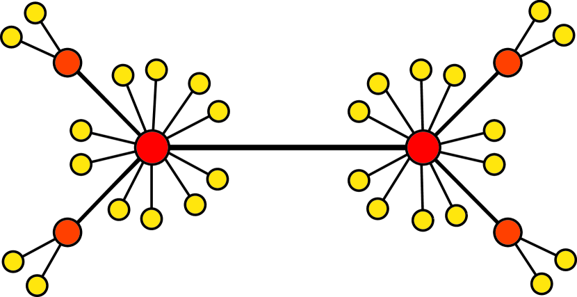
Figure 1: A sketch of G(2,1).

$G^{(0)}$ is a chain of length $1$ where two vertices are connected by an edge of unit weight. For $t>0$, $G^{(t)}$ is obtained from $G^{(t-1)}$ by the following transformation. For each edge of weight $w$ in $G^{(t-1)}$, $mw(m>0)$ new vertices are connected to both sides of the edge respectively with unit weight, meanwhile, the weight of the old edge is increased by $m\theta w(\theta\geqslant 0)$. The parameters $m,\theta$ are all integers. Let $G(m,\theta)=\lim\limits_{t\rightarrow\infty}G^{(t)}$. An infinite branching structure forms.

By construction, the total number of the vertices for $G^{(t)}$ is

$$N_{t}=\frac{2}{2+\theta}[(\theta m+2m+1)^{t}+\theta+1].$$ (1)

Name these vertices by $v_{1},v_{2},\cdots,v_{N_{t}}$. $a_{ij}$ denotes the weight of the edge connecting $v_{i}$ and $v_{j}$. $a_{ij}$ is $0$ when $v_{i}$ and $v_{j}$ are not adjacent. Further we define the degree of $v_{i}$ as $d_{i}=\sum_{j}a_{ij}$.

To describe the topological structure of $G^{(t)}$, we introduce the adjacency matrix $(A^{(t)})_{ij}=a_{ij}$ and the degree matrix $(D^{(t)})_{ij}=\delta_{ij}d_{i}$. Let the normalized stochastic matrix Chen and Zhang (2007) for markov chains on $G^{(t)}$ be $T^{(t)}=\sqrt{D^{(t)}}A^{(t)}\sqrt{D^{(t)}}$. Obviously, $t_{ij}=\frac{a_{ij}}{\sqrt{d_{i}d_{j}}}$. For $G(m,\theta)$, define $T=\lim\limits_{t\rightarrow\infty}T^{(t)}$.

III Tight-binding model on $G(m,\theta)$

Suppose the structure we constructed denotes a trapping structure for quantum gases. The edges connecting two vertices represent the correlation of two traps. The tight-binding Hamiltonian describing the system writes Serva (2014); de Oliveira et al. (2013)

$$\hat{\mathcal{H}_{0}}=\sum_{i}d_{i}\hat{a}_{i}^{\dagger}\hat{a}_{i}-\sum_{ij}a_{ij}\hat{a}_{i}^{\dagger}\hat{a}_{j}.$$ (2)

Here $\hat{a}_{i}^{\dagger}$ and $\hat{a}_{i}$ are creation and annihilation operators and $a_{ij}$ denotes the hopping amplitude between two coupled traps. The second summation in Eq. (2) is taken over all neighboring vertices $i$ and $j$. Clearly, when $\theta=0$, $a_{ij}$ is constantly 1 for all existing site-site correlations. This is the most homogeneous case in our model. For non-vanishing $\theta$, the hopping amplitude is heterogeneous.

From Eq. (2), we know the spectrum of $\hat{\mathcal{H}_{0}}$ is unbound for infinite network($t\rightarrow\infty$). However, by rescaling the frequency space(multiplying the Hamiltonian by diagonal operators at both sides), we can normalize $\hat{\mathcal{H}_{0}}$ as

$$\hat{\mathcal{H}}=-\sum_{ij}t_{ij}\hat{a}_{i}^{\dagger}\hat{a}_{j},$$ (3)

of which the spectrum lies on $[-1,1]$.

The matrix $T$ we defined previously hence gives a full description of $\hat{\mathcal{H}}$. The allowed energy for $\hat{\mathcal{H}}$ is the eigenvalue spectrum of $-T$. The spectrum is a Julia multiset $J_{R}\subset[-1,1]$ generated by the inverse of the function

$$R(x)=\frac{\theta m+m+1}{\theta m+1}x-\frac{m}{(\theta m+1)x}$$ (4)

from $\{-1,1\}\bigcup\{0\}$ Teplyaev (1998); Hare et al. (2012). A detailed description of $J_{R}$ is provided in the appendix. Fig. 2 shows how the eigenvalue spectra vary with the weight parameter $\theta$. When $\theta\rightarrow\infty$, the spectrum is dense in $[-1,1]$.

Let $\textrm{deg}^{(t)}(\varepsilon)$ denote the multiplicity of the eigenvalue $\varepsilon$ of $-T^{(t)}$. Take $\textrm{deg}^{(t)}(\varepsilon)=0$ if $\varepsilon$ is not an eigenvalue. The density of states on $[-1,1]$ is

$$\rho(\varepsilon)=\sum_{\varepsilon^{\prime}\in J_{R}}\delta(\varepsilon-\varepsilon^{\prime})\lim_{t\rightarrow\infty}\frac{\textrm{deg}^{(t)}(\varepsilon^{\prime})}{N_{t}}$$ (5)

where $\delta(\varepsilon-\varepsilon^{\prime})$ is the Dirac delta function. Fig. 3 is a schematic representation of $\rho(\epsilon)$ related to different $\theta$. Obviously, $\rho(\epsilon)$ shows self-similar properties.

Fig. 2 and Fig. 3 together show that the spectrum related to $G(m,\theta)$ is highly degenerate and fractal-like. Besides, the spectrum is symmetric with respect to $\epsilon=0$ , which possesses the largest degeneracy. From Fig. 2, we have also found several isolated levels, among which $\epsilon=0$ is fixed for any $\theta$.

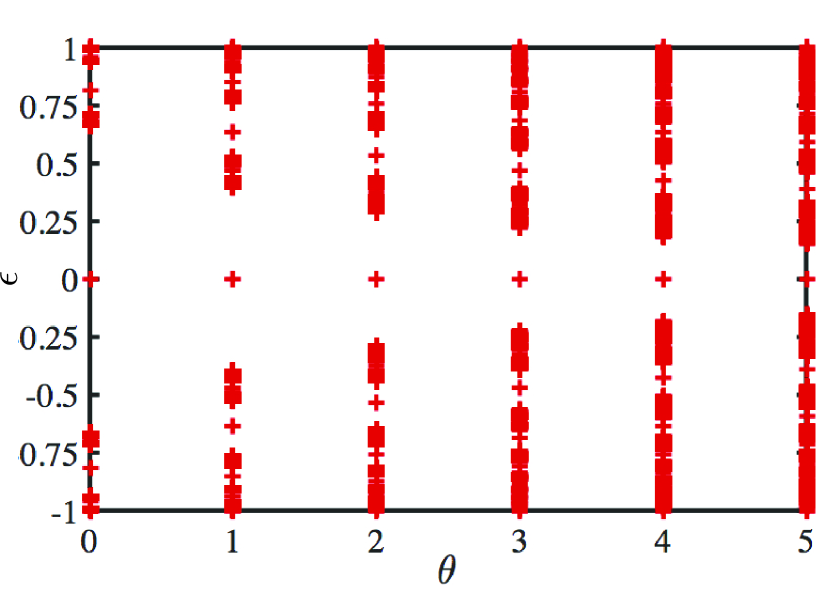
Figure 2: (Color online) Eigenvalue spectra related to $\theta$ from $0$ to $6$ when $m=2$.

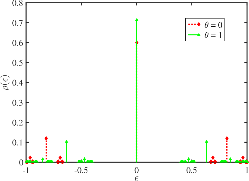
Figure 3: (Color online) Density of states associated to $G(2,0)$ and $G(2,1)$.

The integrated density of states is defined as

$$I(\varepsilon)=\int_{-1}^{\varepsilon}\rho(x)dx.$$ (6)

Since the smallest eigenvalue of $-T$ is always $-1$ through iteration, the lowest allowed energy for $\hat{\mathcal{H}}$ is $\varepsilon_{0}=-1$. Near the lowest energy level, the power-law behavior of the integrated density of states is observed, given by

$$I(\varepsilon)\sim(\varepsilon-\varepsilon_{0})^{\frac{d_{s}}{2}}.$$ (7)

$d_{s}$ is called the spectral dimension of $G(m,\theta)$, working as a generalization of the Euclidean dimension defined on homogeneous systems such as regular lattices Rammal (1984); Alexander and Orbach (1982); Cassi and Regina (1993).

Under iteration, the energy level near the bottom is stable ($R(-1)=-1$) and the integrated density of states is fixed, one obtains

$$\lim_{\begin{subarray}{c}t\rightarrow\infty\\ \varepsilon\rightarrow-1\end{subarray}}\frac{N_{t+1}}{N_{t}}\frac{I(\varepsilon)}{I\left(R(\varepsilon)\right)}=1.$$ (8)

Plugging Eq. (7) into Eq. (8), after some algebra we arrive at

$$d_{s}=2\frac{\ln(\theta m+2m+1)}{\ln(\theta m+2m+1)-\ln(\theta m+1)}.$$ (9)

Obviously, $d_{s}\geqslant 2$, where the equality only holds for $\theta=0$.

IV Fermi gas on $G(m,\theta)$

In this section we will study the behaviors of non-interacting hopping fermions trapped by the structure we have constructed. The Hamiltonian for the system is still given by Eq. (3) while the creation and annihilation operators are fermionic now. We ignore spins for evident reasons.

The Fermi-Dirac statistics give the average occupation number of each state with energy $\epsilon$:

$$\bar{n}(\epsilon)=\frac{1}{e^{\beta(\epsilon-\mu)}+1}.$$ (10)

In Eq. (10), $\beta=\frac{1}{k_{B}T}$ and $\mu$ is the chemical potential. The normalization condition requires

$$\int_{-1}^{1}\bar{n}(\epsilon)\rho(\epsilon)d\epsilon=\gamma$$ (11)

where $\gamma>0$ is the filling fraction, i.e., the ratio of particles to vertices.

Let $E_{F}$ denote the Fermi energy of this system.

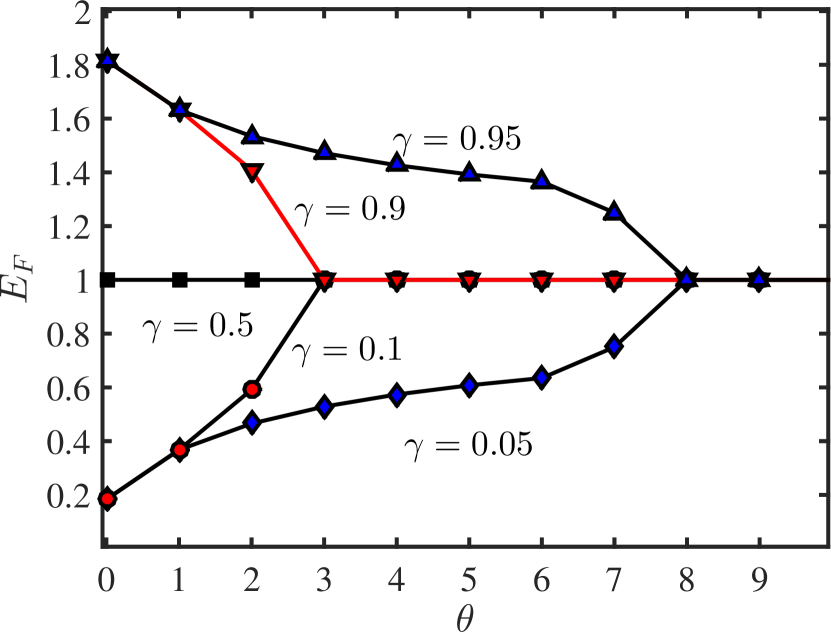
Figure 4: (Color online) The relation between $E_{F}$ and $\theta$ for $G(2,\theta)$.

To investigate the influence of the parameter $\theta$ on the Fermi energy while the structural parameter $m$ is fixed, we put $m=2$ without loss of generality. The dependence of $E_{F}$ on $\theta$ is given in Fig. 4. Except for half filling, $E_{F}$ varies with $\theta$ for fixed $\gamma$ and low $\theta$ due to the huge degeneracy of $\epsilon=0$. We can also give the range of $\gamma$ that allows $E_{F}=1$ as $\gamma\in[\gamma_{c}(m,\theta),1-\gamma_{c}(m,\theta)]$. $\gamma_{c}(m,\theta)$ is determined by checking the weight of level $\epsilon=0$:

$$1-2\gamma_{c}(m,\theta)=\lim_{t\rightarrow\infty}\frac{\textrm{deg}^{(t)}(\varepsilon=0)}{N_{t}}.$$ (12)

Eq. 12 yields $\gamma_{c}(m,\theta)=\frac{1}{\theta m+2m+1}$. As $\theta\rightarrow\infty$, $\gamma\rightarrow 0$ since the level $\epsilon=0$ predominates.

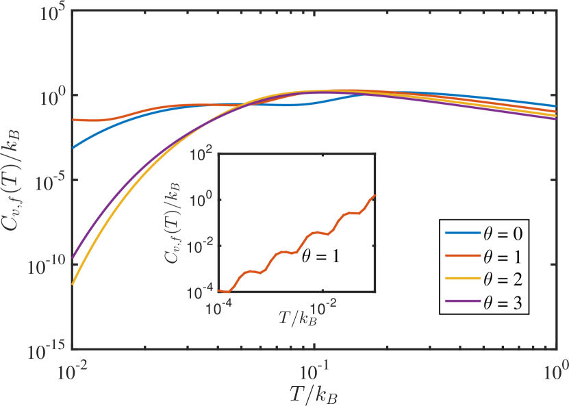
Figure 5: (Color online) Specific heat as a function of the temperature for $\theta=0,1,2,3$ ($m=2,\gamma=0.125$). The inset shows the oscillating decay of $C_{v,f}(T)$ as $T\rightarrow 0$ when $\theta=1$.

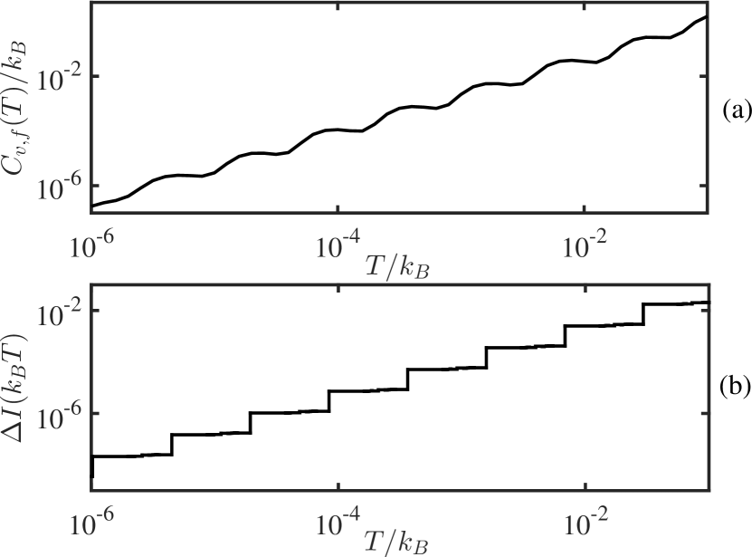
Figure 6: (a) Log-log plot of the specific heat versus the temperature ($m=2,\theta=1,\gamma=0.125$). (b) Log-log plot of $\Delta I(k_{B}T)=I(\epsilon_{0}+E_{F}+k_{B}T)-I(\epsilon_{0}+E_{F}-k_{B}T)$ versus the temperature ($m=2,\theta=1,\gamma=0.125$). The two curves display the same periodicity.

Next we pay attention to the thermodynamic property of the system.

The average internal energy per particle is $U=\frac{1}{\gamma}\int_{-1}^{1}\bar{n}(\epsilon)\rho(\epsilon)\epsilon d\epsilon$. Subsequently the heat capacity per particle or specific heat is

$$C_{v,f}(T)=\frac{dU}{dT}=\frac{k_{B}\beta^{2}}{4}\left(<\epsilon^{2}\rho(\epsilon)>_{{}_{f}}-\frac{<\epsilon\rho(\epsilon)>_{{}_{f}}^{2}}{<\rho(\epsilon)>_{{}_{f}}}\right)$$ (13)

where $<g(\epsilon)>_{{}_{f}}$ denotes the integral

$$<g(\epsilon)>_{{}_{f}}=\int_{-1}^{1}\frac{g(\epsilon)d\epsilon}{\cosh^{2}\frac{\beta(\epsilon-\mu)}{2}}.$$ (14)

A schematic representation of the specific heat as a function of temperature is given in Fig. 5. In low-temperature approximation, Eq. (13) becomes

$$C_{v,f}(T)=\frac{k_{B}\beta^{2}}{4}\left(<(\epsilon-E_{F})^{2}\rho(\epsilon)>_{{}_{f}}-\frac{<(\epsilon-E_{F})\rho(\epsilon)>_{{}_{f}}^{2}}{<\rho(\epsilon)>_{{}_{f}}}\right).$$ (15)

The integral Eq. (14) is approximated by

$$<g(\epsilon)>_{{}_{f}}=\int_{E_{F}-\delta/\beta}^{E_{F}+\delta/\beta}\frac{g(\epsilon)d\epsilon}{\cosh^{2}\frac{\beta(\epsilon-E_{F})}{2}}.$$ (16)

As a rough estimate we can set $1<\delta<10$. Since $\rho(\epsilon)$ is locally symmetric (as shown in Fig. 3) and $(\epsilon-E_{F})/\cosh^{2}\frac{\beta(\epsilon-E_{F})}{2}$ is strictly odd with respect to $\epsilon=E_{F}$, the second term on the right side of Eq. (15) is negligible. Thus

$$C_{v,f}(T)=\frac{k_{B}^{2}T}{4}\int_{-\delta}^{\delta}\frac{t^{2}\rho({tk_{B}T}+\epsilon_{0}+E_{F})dt}{\cosh^{2}\frac{t}{2}}.$$ (17)

If $\epsilon=\epsilon_{0}+E_{F}$ is an isolated point in the energy spectrum, the integral in Eq. (17) is 0. Correspondingly, the curves associated to $\theta=0$ $(E_{F}=0.1835)$, $\theta=2$ $(E_{F}=1)$ and $\theta=3$ $(E_{F}=1)$ in Fig. 5 decay rapidly as $T\rightarrow 0$. On the contrary, the curve associated to $\theta=1$ $(E_{F}=0.5)$ displays oscillating decay as $T\rightarrow 0$, because $\epsilon=\epsilon_{0}+E_{F}=-0.5$ is a limit point in the energy spectrum. This means $\rho(\epsilon)$ behaves scale-invariantly near $\epsilon_{0}+E_{F}$. The period of the oscillation, thus, depends on the periodicity of $\log\int_{-\delta}^{\delta}\rho({tk_{B}T}+\epsilon_{0}+E_{F})dt$ with respect to $\log T$. Fig. 6 gives a schematic representation of such relation. One finds $\log(C_{v,f}(T))$ has the same period as $\log\Delta I(k_{B}T)$ with respect to $\log(T)$ at low temperature. This unique effect relates the low-temperature dependence of the specific heat to the self-similarity of the spectrum straightforwardly. Moreover, this effect is only present for certain degree of heterogeneity of the coupling for fixed $\gamma$. And, in large $\theta$, this effect is only allowed for full filling. Other results regarding the log-periodic oscillation of specific heat can be found at de Oliveira et al. (2009); Aydin and Sisman (2014).

Based on above analysis, the value of the structural parameters $m$, $\theta$ and the filling fraction $\gamma$ together determine the low-temperature dependence of the specific heat. The trivial case occurs when $\gamma\in[\gamma_{c}(m,\theta),1-\gamma_{c}(m,\theta)]$, for which $E_{F}=1$ is a isolated energy. Otherwise we need to check whether $E_{F}$ represents an non-isolated level so that the specific heat will display log-periodic oscillation at low temperature.

V Bose gas on $G(m,\theta)$

As for non-interacting hopping bosons on the same structures, we focus on the low-dimensional Bose-Einstein condensation(BEC) induced by the heterogeneity of site-site coupling. BEC purely arising from topological heterogeneity has been studied before, see Lyra et al. (2014). So here we still keep $m=2$.

Ignoring spin, the average occupation number of each state is given by

$$\bar{n}(\epsilon)=\frac{1}{e^{\beta(\epsilon-\mu)}-1}.$$ (18)

At low temperature, $n_{0}(T)=\frac{1}{e^{\beta(\varepsilon_{0}-\mu)}-1}$ is the number of condensed bosons and $f_{0}(T)=n_{0}(T)/N_{t}$ the condensed fraction.

The normalization condition is still Eq. (11). And the specific heat is

$$C_{v,b}=\frac{k_{B}\beta^{2}}{4}\left(<\epsilon^{2}\rho(\epsilon)>_{{}_{b}}-\frac{<\epsilon\rho(\epsilon)>_{{}_{b}}^{2}}{<\rho(\epsilon)>_{{}_{b}}}\right)$$ (19)

where $<g(\epsilon)>_{{}_{f}}$ denotes the integral

$$<g(\epsilon)>_{{}_{b}}=\int_{-1}^{1}\frac{g(\epsilon)d\epsilon}{\sinh^{2}\frac{\beta(\epsilon-\mu)}{2}}.$$ (20)

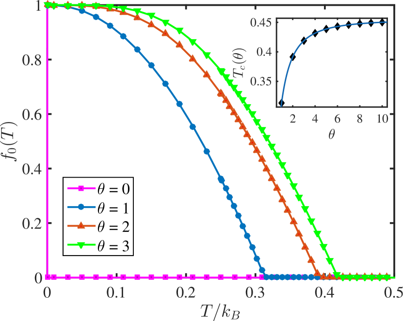
Figure 7: (Color online) Condensed fraction as a function of temperature for $\theta=0$ $(d_{s}=2)$, $1$ $(d_{s}=4.593)$, $2$ $(d_{s}=7.476)$, $3$ $(d_{s}=10.610)$ when the filling fraction is $\gamma=1/8$. For $\theta>0$, Bose-Einstein condensation is detected. The inset displays the transition temperature as a function of $\theta$ for $\gamma=1/8$. It is saturated as $\theta\rightarrow\infty$.

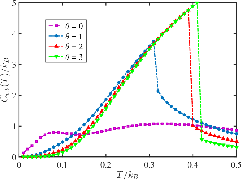
Figure 8: (Color online) Specific as a function of temperature $\theta=0,1,2,3$ when $\gamma=1/8$. $C_{v,b}(T)$ has jump discontinuity at the transition temperature for $\theta>0$.

A schematic representation of the relation between the condensed fraction and the temperature is given by Fig. 7, where we find the value of $\theta$ determines the occurrence of BEC and the transition temperature. The corresponding relation between the specific heat and the temperature is shown in Fig. 8. It is clear that BEC occurs only for non-vanishing $\theta$. In Fig. 8 we also observe that the curves associated to $\theta>0$ have jump discontinuities, indicating the location of the transition temperature. Obviously, the transition temperature $T_{c}(\theta)$ increases monotonically and saturates when $\theta\rightarrow\infty$, as shown in the inset of Fig. 7. As one can predict, the critical relation for condensed fraction is $f_{0}(T)\propto\frac{T_{c}-T}{Tc}$ near the critical temperature.

Through Eq. (9) we find the spectral dimension related to $\theta=0$ is always $2$ no matter how large $m$ is. Since BEC is forbidden for spectral dimension not larger than 2, BEC does not take place upon $G(m,0)$ that is the homogeneous configuration. This conclusion exactly reflects the importance of the heterogeneity of the site-site coupling strength instead of the heterogeneity in topological structures. Because the latter fails to induce a phase transition.

VI Conclusion

Though it may be satisfactory to study homogeneous model for many real-world solids when disorder is introduced, the non-uniform model is necessary for plenty of other applications as we have mentioned in Sec. I. In this spirit, we investigated trapped non-interacting bosons and fermions upon a scale-invariant trap structure, with the branching parameter $m$ and the weight parameter $\theta$ controlling the heterogeneity of the site-site coupling strength. Through exact renormalization, we analytically determined the entire energy spectrum of the normalized Hamiltonian with tight-binding approximation. The spectrum was shaped by the value of $\theta$. Then we studied the unique thermodynamic behaviors of our model at low temperature with different degree of heterogeneity. To fermions, log-periodic oscillation of specific heat only occurs for certain $\theta$ provided fixed filling fraction. To bosons, the Bose-Einstein condensation is forbidden for the homogeneous setup($\theta=0$) regardless of the value of $m$.

The scale-invariant branching structure in this study is exactly renormalizable hence allows efficient analytical study. At the same time other irregular structures can not enjoy such convenience. Nevertheless, the deterministic renormalizable structures give us precious insight into the heterogeneity of network-like structures. Be more specific, our model serves as a good prototype for plenty of scale-invariant models all displaying fractal-like spectra Cardoso et al. (2008); Nandy et al. (2014). In fact one can distort a solved structure while keeping the emergent behaviors unchanged. For example, the branching parameter $m$ in our model can actually vary with different branches while keeping BEC forbidden for $\theta=0$.

As a final comment, if we regard the topological aspect of structural heterogeneity as the shape of a circuit, the heterogeneity in site-site couplings alters the distribution of resistance. The latter puts the emphasis on some parts of a lattice and weakens the rest. In this circumstance, more features are added to a model that is previously uniform. This is the reason why we can find lots of interesting phenomena in the simplest model we consider here.

Appendix

For clarity, name the vertex set of $G^{(t)}$ by $V_{t}$. The set of the new nodes generated at iteration $t+1$ is denoted by $V_{t+1}\backslash V_{t}$. By proper arranging $T^{(t+1)}$ can be expressed as

$$T^{(t+1)}=\left(\begin{matrix}\frac{\theta m+1}{\theta m+m+1}T^{(t)}&S\\ S^{T}&0\end{matrix}\right).$$ (21)

In Eq. (21) $S$ reflects the coupling between the new vertices generated at iteration $t+1$ and the rest. Correspondingly partition the eigenvector of $T^{(t+1)}$ as $\psi=(\phi,\varphi)$ with respect to eigenvalue $\lambda$. Hence

$$\frac{\theta m+1}{\theta m+m+1}T^{(t)} \phi+S\varphi =\lambda\phi$$ (22)

$$S^{T} \phi =\lambda\varphi,$$ (23)

which yields

$$\bigg{(}\frac{\lambda(\theta m+1)}{\theta m+m+1}T^{(t)}+SS^{T}-\lambda^{2}\bigg{)}\phi=0$$ (24)

provided $\lambda\neq 0$.

By the construction procedure,

$$(SS^{T})_{ij}=\sum_{v_{k}\in V_{t+1}\backslash V_{t}}S_{ik}S_{jk}=\sum_{v_{k}\in V_{t+1}\backslash V_{t}}\frac{a_{ik}a_{jk}}{d_{k}\sqrt{d_{i}d_{j}}}$$ (25)

is nonzero if and only if $i=j$ since each $v_{k}$ is adjacent to one vertex only. By simple algebra one arrives at

$$(SS^{T})_{ii}=\frac{m}{\theta m+m+1}.$$ (26)

Due to Eq. (26), Eq. (24) is simplified as

$$\left(T^{(t)}-\frac{\theta m+m+1}{\theta m+1}\lambda+\frac{m}{(\theta m+1)\lambda}\right)\phi=0$$ (27)

which entails

$$R(\lambda)=\frac{\theta m+m+1}{\theta m+1}\lambda-\frac{m}{(\theta m+1)\lambda}.$$ (28)

$R(\lambda)$ is the eigenvalue of $T^{(t)}$ associated to eigenvector $\phi$. Further one will find the multiplicity of $R(\lambda)$ to $T^{(t)}$ is the same as the multiplicity of $\lambda$ to $T^{(t+1)}$.

Without proof we claim that the preimage of $\lambda$ under function $R$ is a subset of the eigenvalue spectrum of $T^{(t+1)}$. Any eigenvalue in the preimage of $\lambda$ carries on the multiplicity of $\lambda$. Notice that by tracking the preimage of the spectrum $T^{(t)}$ under function $R$ one can obtain only $2N_{t}$ eigenvalues of $T^{(t+1)}$. Fortunately, the left $N_{t+1}-2N_{t}$ eigenvalues are uniformly 0 that is the only singularity of $R$. More detailed discussion about the iterative derivation of spectrum can be found at Xie et al. (2016, 2015).

So far we are able to obtain the full spectrum of $T^{(t)}$ by tracking the flow generated by $R$. As $t\rightarrow\infty$, the spectrum grows into a Julia set $J_{R}$ given as

$$J_{R}=\{0\}\bigcup\lim_{n\rightarrow\infty}R^{-n}(\{1,-1,0\}).$$ (29)

As for $-T$, the result is the same since the spectrum of $T$ is symmetric about $0$.

References

- Cardoso et al. (2008) A. L. Cardoso, R. F. S. Andrade, and A. M. C. Souza, Phys. Rev. B 78, 214202 (2008).
- Nandy et al. (2014) A. Nandy, B. Pal, and A. Chakrabarti, Phys. Lett. A 378, 3144 (2014).
- Yamada (2015) H. S. Yamada, Eur. Phys. J. B 88, 264 (2015).
- Jana et al. (2010) S. Jana, A. Chakrabarti, and S. Chattopadhyay, Phys. B Condens. Matter 405, 3735 (2010).
- Chakrabarti (2011) A. Chakrabarti, Phys. Lett. A 375, 3899 (2011).
- van Veen et al. (2016) E. van Veen, S. Yuan, M. I. Katsnelson, M. Polini, and A. Tomadin, Phys. Rev. B 93, 115428 (2016).
- Moreira et al. (2008) D. Moreira, E. Albuquerque, L. da Silva, and D. Galvao, Phys. A Stat. Mech. its Appl. 387, 5477 (2008).
- Mauriz et al. (2001) P. Mauriz, E. Albuquerque, and M. Vasconcelos, Phys. A Stat. Mech. its Appl. 294, 403 (2001).
- de Oliveira et al. (2004) I. de Oliveira, M. Lyra, and E. Albuquerque, Phys. A Stat. Mech. its Appl. 343, 424 (2004).
- Coronado and Carpena (2005) A. V. Coronado and P. Carpena, Phys. A Stat. Mech. its Appl. 358, 299 (2005).
- Mauriz et al. (2003) P. W. Mauriz, M. S. Vasconcelos, and E. L. Albuquerque, Phys. A Stat. Mech. its Appl. 329, 101 (2003).
- Vallejos and Anteneodo (1998) R. O. Vallejos and C. Anteneodo, Phys. Rev. E 58, 4134 (1998).
- de Oliveira et al. (2009) I. N. de Oliveira, F. A. B. F. de Moura, M. L. Lyra, J. S. Andrade, and E. L. Albuquerque, Phys. Rev. E 79, 016104 (2009).
- Aydin and Sisman (2014) A. Aydin and A. Sisman, Phys. Lett. Sect. A Gen. At. Solid State Phys. 378, 2001 (2014), arXiv:1408.1086 .
- Vidal et al. (2011) E. J. G. G. Vidal, R. P. A. Lima, and M. L. Lyra, Phys. Rev. E 83, 061137 (2011).
- Ketterle and van Druten (1996) W. Ketterle and N. J. van Druten, Phys. Rev. A 54, 656 (1996).
- Burioni et al. (2001) R. Burioni, D. Cassi, M. Rasetti, P. Sodano, and A. Vezzani, J. Phys. B At. Mol. Opt. Phys. 34, 4697 (2001).
- de Oliveira et al. (2013) I. N. de Oliveira, T. B. dos Santos, F. A. B. F. de Moura, M. L. Lyra, and M. Serva, Phys. Rev. E 88, 022139 (2013).
- Bagnato and Kleppner (1991) V. Bagnato and D. Kleppner, Phys. Rev. A 44, 7439 (1991).
- Buonsante et al. (2002) P. Buonsante, R. Burioni, D. Cassi, and A. Vezzani, Phys. Rev. B 66, 094207 (2002).
- Serva (2014) M. Serva, J. Stat. Mech. Theory Exp. 2014, P08018 (2014).
- Brunelli et al. (2004) I. Brunelli, G. Giusiano, F. P. Mancini, P. Sodano, and A. Trombettoni, J. Phys. B At. Mol. Opt. Phys. 37, S275 (2004).
- Lyra et al. (2014) M. L. Lyra, F. A. B. F. de Moura, I. N. de Oliveira, and M. Serva, Phys. Rev. E 89, 052133 (2014).
- Cassi and Regina (1993) D. Cassi and S. Regina, Phys. Rev. Lett. 70, 1647 (1993).
- Burioni and Cassi (1996) R. Burioni and D. Cassi, Phys. Rev. Lett. 76, 1091 (1996).
- Rammal and Toulouse (1983) R. Rammal and G. Toulouse, J. Phys. Lett. 44, 13 (1983).
- Rammal (1984) R. Rammal, J. Phys. 45, 191 (1984).
- Alexander and Orbach (1982) S. Alexander and R. Orbach, J. Phys. Lett. 43, 625 (1982).
- Burioni et al. (1999) R. Burioni, D. Cassi, and S. Regina, Phys. A Stat. Mech. its Appl. 265, 323 (1999).
- Yang and Zhou (2012) Z. Yang and T. Zhou, Phys. Rev. E 85, 056106 (2012).
- Chu et al. (2011) X. Chu, Z. Zhang, J. Guan, and S. Zhou, Phys. A Stat. Mech. its Appl. 390, 471 (2011).
- Wu et al. (2013) Z. Wu, B. Hou, and H. Zhang, Eur. Phys. J. B 86, 405 (2013).
- Soh et al. (2010) H. Soh, S. Lim, T. Zhang, X. Fu, G. K. K. Lee, T. G. G. Hung, P. Di, S. Prakasam, and L. Wong, Phys. A Stat. Mech. its Appl. 389, 5852 (2010).
- Lu et al. (2006) X. B. Lu, X. F. Wang, X. Li, and J. Q. Fang, Phys. A Stat. Mech. its Appl. 370, 381 (2006).
- Huang (2006) D. Huang, Phys. Rev. E 74, 046208 (2006).
- Lin and Zhang (2013) Y. Lin and Z. Zhang, Phys. Rev. E 87, 1 (2013), arXiv:arXiv:1307.0903v1 .
- Zhang et al. (2013) Z. Zhang, T. Shan, and G. Chen, Phys. Rev. E 87, 012112 (2013), arXiv:arXiv:1212.5998v1 .
- Baronchelli and Pastor-Satorras (2010) A. Baronchelli and R. Pastor-Satorras, Phys. Rev. E 82, 011111 (2010).
- Baronchelli et al. (2011) A. Baronchelli, C. Castellano, and R. Pastor-Satorras, Phys. Rev. E 83, 066117 (2011).
- Suchecki et al. (2005) K. Suchecki, V. M. Eguíluz, and M. San Miguel, Phys. Rev. E 72, 036132 (2005).
- Chen and Zhang (2007) H. Chen and F. Zhang, Discret. Appl. Math. 155, 654 (2007).
- Teplyaev (1998) A. Teplyaev, J. Funct. Anal. 159, 537 (1998).
- Hare et al. (2012) K. E. Hare, B. A. Steinhurst, A. Teplyaev, and D. Zhou, Math. Res. Lett. 19, 537 (2012).
- Tsallis et al. (1997) C. Tsallis, L. R. da Silva, R. S. Mendes, R. O. Vallejos, and A. M. Mariz, Phys. Rev. E 56, R4922 (1997).
- Xie et al. (2015) P. Xie, Y. Lin, and Z. Zhang, J. Chem. Phys. 142 (2015), 10.1063/1.4922265.
- Xie et al. (2016) P. Xie, Z. Zhang, and F. Comellas, Appl. Math. Comput. 286, 250 (2016).