The shear and bulk relaxation times from the general correlation functions

Abstract

In this paper we present two quantum field theoretical analyses on the shear and bulk relaxation times. First, we discuss how to find Kubo formulas for the shear and the bulk relaxation times. Next, we provide results on the shear viscosity relaxation time obtained within the diagrammatic approach for the massless $\lambda\phi^{4}$ theory.

1 Introduction

Over the course of last decades relativistic viscous hydrodynamics has been shown to successfully describe and explain the behavior of the strongly interacting matter produced in heavy-ion collisions at the Relativistic Heavy Ion Collider (RHIC) and the Large Hadron Collider (LHC), see Refs. [1, 2] and references therein. In general, any viscous fluid is characterized by a set of transport coefficients. These enter hydrodynamic equations as parameters and must be obtained from the underlying microscopic theory, either in quantum field theory or kinetic theory. Many approaches have been developed to study the first-order transport coefficients [3]-[11] for various systems. There are also some studies on second-order transport coefficients [12]-[22] but their quantum-field-theoretical determination does not seem to be complete.

We have already undertaken the task to study the shear and the bulk relaxation times consistently from first principles. The comprehensive analysis is shown in [23] and here only a brief summary is presented. Using general properties of Green functions and the gravitational Ward identity we first parametrize the stress-energy correlation functions to find their most general forms. Then Kubo formulas for the relaxation times are found in the hydrodynamic limits of the corresponding response functions. We also study shear effects in the massless scalar field theory $\lambda\phi^{4}$ and calculate the shear relaxation time within the real-time formalism.

2 Equations of viscous hydrodynamics

The behavior of a relativistic system, which is close to thermal equilibrium, can be well described by the viscous hydrodynamics, which is based on the energy-momentum conservation law

$$\partial_{\mu}T^{\mu\nu} = 0,$$ (1)

where the energy-momentum tensor takes the form

$$T^{\mu\nu}=\epsilon u^{\mu}u^{\nu}-\Delta^{\mu\nu}(P+\Pi)+\pi^{\mu\nu}$$ (2)

with $\epsilon$ being the energy density, $P$ - thermodynamic pressure, $u^{\mu}$ are the components of the flow velocity with the normalization condition $u^{\mu}u_{\mu}=1$, $\Delta^{\mu\nu}=g^{\mu\nu}-u^{\mu}u^{\nu}$ is the projection operator with $u_{\mu}\Delta^{\mu\nu}=0$, and the Minkowski metric is $g^{\mu\nu}=(1,-1,-1,-1)$. The terms $\Pi$ and $\pi^{\mu\nu}$ are the bulk viscous pressure and the shear stress tensor, respectively, which have well defined forms in the Navier-Stokes limit. Then the viscous corrections are characterized by the bulk viscosity $\zeta$ and shear viscosity $\eta$, respectively. In the second order formulation of viscous hydrodynamics, the response of medium to the thermodynamic forces is not instantaneous. The viscous corrections approach their corresponding Navier-Stokes forms within some characteristic time scales, which are the bulk and shear relaxation times, $\tau_{\Pi}$ and $\tau_{\pi}$. Consequently, the viscous corrections are subject to relaxation equations

$$\Pi=\Pi_{NS}-\tau_{\Pi}\dot{\Pi},\qquad\qquad\qquad\pi^{\mu\nu}=\pi^{\mu\nu}_{NS}-\tau_{\pi}\dot{\pi}^{\langle\mu\nu\rangle},$$ (3)

where $\Pi_{NS}$ and $\pi^{\mu\nu}_{NS}$ are the bulk pressure and the stress tensor in the Navier-Stokes approach, and we used the notation $A^{\langle\mu\nu\rangle}\equiv\Delta^{\mu\nu}_{\alpha\beta}A^{\alpha\beta}$ where $\Delta^{\mu\nu}_{\alpha\beta}\equiv(\Delta^{\mu}_{\alpha}\Delta^{\nu}_{\beta}+\Delta^{\mu}_{\beta}\Delta^{\nu}_{\alpha}-2/3\Delta^{\mu\nu}\Delta_{\alpha\beta})/2$. We will not consider the non-linear terms here. For more advanced studies on the hydrodynamic equations see, for example, [24].

In case when there are no other than energy and momentum currents occurring in the system, two hydrodynamic modes determine its dynamics. They are governed by the following dispersion relations

$$0 = -\omega^{2}\tau_{\pi}-i\omega+D_{T}{\bf k}^{2}$$ (4)

$$0 = -\omega^{2}+v_{s}^{2}{\bf k}^{2}+i\omega^{3}(\tau_{\pi}+\tau_{\Pi})-i\bigg{(}\frac{4D_{T}}{3}+\gamma+v_{s}^{2}(\tau_{\pi}+\tau_{\Pi})\bigg{)}\omega{\bf k}^{2}$$

$$+\tau_{\pi}\tau_{\Pi}\omega^{4}-\tau_{\pi}\tau_{\Pi}v_{s}^{2}\omega^{2}{\bf k}^{2}-\tau_{\Pi}\frac{4D_{T}}{3}\omega^{2}{\bf k}^{2}-\tau_{\pi}\gamma\omega^{2}{\bf k}^{2},$$

where $\omega$ and ${\bf k}$ are the frequency and wavevector of the modes, $D_{T}=\eta/(\epsilon+P)$, $\gamma=\zeta/(\epsilon+P)$, and $v_{s}^{2}=\partial P/\partial\epsilon$ is the speed of sound squared. The dispersion relation (4) governs the propagation of the diffusion mode which occurs in the direction transverse to the the flow velocity. The sound mode is, in turn, given by the dispersion relation (2) and it is an effect of the small disturbances propagating longitudinally in the medium. Both dispersion relations are essential to determine the respective correlation functions of the stress-energy tensor.

3 Stress-energy correlation functions and Kubo formulas

Since viscous hydrodynamics is a manifestation of the linear response theory, the deviations of different observables are given in terms of corresponding equilibrium response functions. Therefore, the response functions carry dynamical information about the system. In general, these functions cannot be calculated exactly but one is able to parametrize their most general structures for the stress-energy tensor components using the following arguments. First, the real part of a correlation function is an even function of frequency and the imaginary part, which directly corresponds to the spectral function, must be an odd function of frequency. Next, since the stress-energy tensor represents at the same time the conserved currents and also generators of the space time evolution, its correlation functions must satisfy the gravitational Ward identity [25]

$$k_{\alpha}\big{(}\bar{G}^{\alpha\beta,\mu\nu}(k)-g^{\beta\mu}\langle\hat{T}^{\alpha\nu}\rangle-g^{\beta\nu}\langle\hat{T}^{\alpha\mu}\rangle+g^{\alpha\beta}\langle\hat{T}^{\mu\nu}\rangle\big{)}=0.$$ (6)

Finally, the low-frequency and long-wavelength limits must be properly incorporated to ensure the correlation functions behave well in these limits.

Using aforementioned arguments we have parametrized the retarded Green function for the shear flow as

$$\bar{G}_{R}^{xy,xy}(\omega,k_{y})=\frac{\omega^{2}(\epsilon+g_{T}(k_{y})+i\omega A(\omega,k_{y}))}{k_{y}^{2}-i\omega/D(\omega,k_{y})-\omega^{2}B(\omega,k_{y})}-P,$$ (7)

where $g_{T}(k_{y})=P+g_{\pi\pi}(k_{y})$ with $g_{\pi\pi}(k_{y})$ being a function of $k_{y}$ of the order at least $O(k_{y}^{2})$ in the small $k_{y}$ limit. The functions $A$, $B$, and $D$ have the form $D(\omega,k_{y})=D_{R}(\omega,k_{y})-i\omega D_{I}(\omega,k_{y})$, where $D_{R}(\omega,k_{y})$ and $D_{I}(\omega,k_{y})$ are real-valued even functions of $\omega$ and $k_{y}$. The real parts $D_{R}$ and $B_{R}$ must have a non-zero limit as $\omega\rightarrow 0$ and $k_{y}\rightarrow 0$. All other parts of $A$, $B$, and $D$ must have finite limits as $\omega\rightarrow 0$ and $k_{y}\rightarrow 0$. By matching the denominator of the Eq. (7) to the dispersion relation (4) one is able to express $D_{R}$, $D_{I}$, $B_{R}$, etc in the hydrodynamic limits via the transport coefficients and obtain the following Kubo relations

$$\eta=\lim_{\omega\rightarrow 0}\lim_{k_{y}\rightarrow 0}\frac{1}{\omega}\textrm{Im}\bar{G}_{R}^{xy,xy}(\omega,k_{y}),\qquad\qquad\qquad\eta\tau_{\pi}-\frac{\kappa}{2}=-\frac{1}{2}\lim_{\omega\rightarrow 0}\lim_{k_{y}\rightarrow 0}\partial_{\omega}^{2}\;\textrm{Re}\bar{G}_{R}^{xy,xy}(\omega,k_{y}),$$ (8)

where $\kappa$ is the static susceptibility. Accordingly, both formulas have to be used to find the shear relaxation time in the leading order. The coefficient $\kappa$ was shown in [26, 27] to be $\kappa=\mathcal{O}(\lambda^{0}T^{2})$ in the weak coupling limit. On the other hand, both $\eta$ and $\tau_{\pi}$ are related to the mean free path which depends inversely on the coupling constant. Hence, $\kappa$ may be omitted in further analysis.

To examine the bulk viscosity and its relaxation time one needs to consider the response function to the longitudinal fluctuations. Employing the analogous procedure as in case of shear flow we obtain the most general form of the longitudinal fluctuation correlation function in the form

$$\bar{G}_{L}(\omega,{\bf k})=\frac{\omega^{2}(\epsilon+P+\omega^{2}Q(\omega,{\bf k}))}{{\bf k}^{2}-\omega^{2}/Z(\omega,{\bf k})+i\omega^{3}R(\omega,{\bf k})},$$ (9)

where the functions $Q$, $R$, and $Z$ are constrained in a similar way as the functions $A$, $B$, and $D$ occurring in Eq. (7). When hydrodynamic limits are applied one obtains some Kubo formulas employing $\zeta$, $\eta$, $\tau_{\Pi}$, $\tau_{\pi}$, and $\kappa$. However, with the help of Eqs. (8) we can extract simple Kubo formulas involving only bulk viscosity and its relaxation time. These are then given in terms of the pressure-pressure correlation function

$$\zeta=\lim_{\omega\rightarrow 0}\lim_{{\bf k}\rightarrow 0}\frac{1}{\omega}\textrm{Im}\,\bar{G}_{R}^{PP}(\omega,{\bf k}),\qquad\qquad\qquad\zeta\tau_{\Pi}=-\frac{1}{2}\lim_{\omega\rightarrow 0}\lim_{{\bf k}\rightarrow 0}\partial^{2}_{\omega}\textrm{Re}\,\bar{G}_{R}^{PP}(\omega,{\bf k}).$$ (10)

These formulas constitute the way of computation of the bulk relaxation time.

4 Shear relaxation time in scalar field theory

It is elastic scatterings that constitutes the shear effects and therefore to evaluate the shear relaxation time within the scalar massless field theory $\lambda\phi^{4}$ one requires expanding the retarded Green function to the leading order. For the comprehensive calculation see [23].

Following Kubo relations one obtains integral equations for the imaginary and real parts of the retarded Green functions, which then are solved numerically and the shear relaxation time is extracted. It has been shown that both the shear viscosity and the relaxation time are related to the inverse of the thermal width, as expected. In the left panel of Fig. 1 the relaxation time is plotted as a function of the thermal mass over temperature and $m_{\textrm{th}}/T$ which should be identified with $\sqrt{\lambda}$ with $\lambda$ being the coupling constant. In the left panel of Fig. 1 we present the ratio $\langle\epsilon+P\rangle\tau_{\pi}/\eta$ as a function of $m_{\textrm{th}}/T$ showing that it changes between 6.11 up to 6.55 in the range shown. The results presented here are in agreement with those obtained within kinetic theory [12, 15].

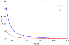
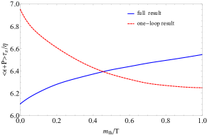
Fig. 1: Left panel: shear relaxation time as a function of $m_{\textrm{th}}/T$. Right panel: the ratio $\langle\epsilon+P\rangle\tau_{\pi}/\eta$ as a function of $m_{\textrm{th}}/T$. Evaluation in the one-loop limit (red dashed curve) and multi-loop resummation (blue curve) are presented.

5 Conclusions

In this article we presented a set of Kubo formulas which enable us to compute the shear and the bulk relaxation times. The main focus was to obtain the Kubo formula to compute the bulk relaxation time and the formula found is consistent with the one obtained via the metric perturbation analysis [22] but it is different from the one obtained from the projection operator method [21].

We also computed the shear relaxation time and the ratio $\langle\epsilon+P\rangle\tau_{\pi}/\eta$ within scalar massless theory and their values are consistent with previous studies. In general the ratio seems to vary between 5 up to 7 across different theories.

References

- [1] C. Gale, S. Jeon and B. Schenke, Int. J. Mod. Phys. A 28, 1340011 (2013)
- [2] U. Heinz and R. Snellings, Ann. Rev. Nucl. Part. Sci. 63, 123 (2013)
- [3] S. Jeon, Phys. Rev. D 47, 4586 (1993)
- [4] S. Jeon, Phys. Rev. D 52, 3591 (1995)
- [5] J. S. Gagnon and S. Jeon, Phys. Rev. D 75, 025014 (2007)
- [6] J. S. Gagnon and S. Jeon, Phys. Rev. D 76, 105019 (2007)
- [7] M. A. Valle Basagoiti, Phys. Rev. D 66, 045005 (2002)
- [8] S. Jeon and L. G. Yaffe, Phys. Rev. D 53, 5799 (1996)
- [9] P. B. Arnold, G. D. Moore and L. G. Yaffe, JHEP 0011, 001 (2000)
- [10] P. B. Arnold, G. D. Moore and L. G. Yaffe, JHEP 0305, 051 (2003)
- [11] P. B. Arnold, G. D. Moore and L. G. Yaffe, JHEP 0301, 030 (2003)
- [12] M. A. York and G. D. Moore, Phys. Rev. D 79, 054011 (2009)
- [13] G. S. Denicol, T. Koide and D. H. Rischke, Phys. Rev. Lett. 105, 162501 (2010)
- [14] G. S. Denicol, H. Niemi, E. Molnar and D. H. Rischke, Phys. Rev. D 85, 114047 (2012) Erratum: [Phys. Rev. D 91, no. 3, 039902 (2015)]
- [15] G. S. Denicol, S. Jeon and C. Gale, Phys. Rev. C 90, no. 2, 024912 (2014)
- [16] G. S. Denicol, J. Noronha, H. Niemi and D. H. Rischke, Phys. Rev. D 83, 074019 (2011)
- [17] G. S. Denicol, J. Noronha, H. Niemi and D. H. Rischke, J. Phys. G 38, 124177 (2011)
- [18] R. Baier, P. Romatschke, D. T. Son, A. O. Starinets and M. A. Stephanov, JHEP 0804, 100 (2008)
- [19] G. D. Moore and K. A. Sohrabi, Phys. Rev. Lett. 106, 122302 (2011)
- [20] T. Koide, E. Nakano and T. Kodama, Phys. Rev. Lett. 103, 052301 (2009)
- [21] X. G. Huang, T. Kodama, T. Koide and D. H. Rischke, Phys. Rev. C 83, 024906 (2011)
- [22] J. Hong and D. Teaney, Phys. Rev. C 82, 044908 (2010)
- [23] A. Czajka and S. Jeon, arXiv:1701.07580 [nucl-th]
- [24] S. Jeon and U. Heinz, Int. J. Mod. Phys. E 24, no. 10, 1530010 (2015)
- [25] S. Deser and D. Boulware, J. Math. Phys. 8, 1468 (1967)
- [26] P. Romatschke and D. T. Son, Phys. Rev. D 80, 065021 (2009)
- [27] G. D. Moore and K. A. Sohrabi, JHEP 1211, 148 (2012)