Consistencies and inconsistencies between model selection and link prediction in networks

Abstract

A principled approach to understand network structures is to formulate generative models. Given a collection of models, however, an outstanding key task is to determine which one provides a more accurate description of the network at hand, discounting statistical fluctuations. This problem can be approached using two principled criteria that at first may seem equivalent: selecting the most plausible model in terms of its posterior probability; or selecting the model with the highest predictive performance in terms of identifying missing links. Here we show that while these two approaches yield consistent results in most of cases, there are also notable instances where they do not, that is, where the most plausible model is not the most predictive. We show that in the latter case the improvement of predictive performance can in fact lead to overfitting both in artificial and empirical settings. Furthermore, we show that, in general, the predictive performance is higher when we average over collections of models that are individually less plausible, than when we consider only the single most plausible model.

I Introduction

Real-world complex systems display nontrivial interaction structures. A principled approach to understand these network structures (and the processes that give rise to them) is to formulate generative models and infer their parameters from data. Unfortunately, for any single empirical network, an unlimited number of models can in principle be formulated. Therefore, we need robust and well-founded approaches to compare models and choose the most appropriate one. Specifically, we need approaches that can identify parsimonious models that avoid both overfitting — when purely stochastic fluctuations are mistakenly incorporated into the structure of overly complicated models — and underfitting — when we mistake statistically significant properties of a network for noise, and wrongly select a model that is too simplistic.

Despite the importance and intricacies of model selection for network data, the problem has not been studied systematically. For years, network models have been compared based on their ability to reproduce certain topological features, such as the clustering coefficient, the degree distribution or the community structure. However, such approaches are not rigorous and are prone to overfitting, since one can always design complicated enough models that reproduce any of these properties with arbitrary precision, but that fail to generalize.

Because of this limitation, it is now becoming common to rely on model-selection approaches that are better suited to strike a balance between over and underfitting. These approaches can be either supervised or unsupervised Murphy (2012). In supervised model selection, we prefer the model with the best capacity to generalize from the data and predict missing observations Clauset et al. (2008); Guimerà and Sales-Pardo (2009); Guimerà et al. (2012). In unsupervised model selection, we prefer the model with the highest probability given the data, which can also be interpreted as the model that most compresses the network Rosvall and Bergstrom (2007); Peixoto (2013); Côme and Latouche (2015); Peixoto (2017).

Both approaches aim to find the most parsimonious model, which captures all the structure in the data without incorporating any of the noise. Because of this, one would intuitively expect these two criteria to agree, especially for asymptotically large networks. Indeed, for much simpler types of (non-network) models, the consistency of both approaches has been rigorously shown in specific asymptotic limits Shao (1993, 1997); Arlot and Celisse (2010). However, their implementations are quite different and, in practice, it is not yet understood in what regimes discrepancies should be expected.

Here, we discuss the probabilistic foundations of supervised and unsupervised model selection, and make a systematic comparison between both approaches using variations of the stochastic block model Holland et al. (1983). We show that the two criteria tend to agree, that is, that the most predictive model tends to be the one that most compresses the data. Crucially, however, we show that it is possible to construct networks where both approaches differ, even in the infinite size limit, and the supervised approach leads to overfitting. In fact, this non-intuitive discrepancy is also observed in some real networks, albeit for a minority of cases.

Moreover, we find that, although in practice the most predictive model is often the one that most compresses the data, the reverse is not true — the most accurate link predictions are not given by the most compressive model but by an average over less compressive ones. Remarkably, for all the networks and models we study, this improvement in predictive power is larger than the improvement obtained using more sophisticated models; or, in other words, averaging over samples of even the simplest models is often more predictive than the single most sophisticated model.

II Probabilistic framework and stochastic block model classes

II.1 Probabilistic framework

Probabilistically, the model selection task consists in finding the model $\mathcal{M}$ that is most likely to have generated a given network with adjacency matrix $\bm{A}$, that is, the model that maximizes $P(\mathcal{M}|\bm{A})$. This probability is the Bayesian posterior

$$P(\mathcal{M}|\bm{A})=\frac{P(\bm{A}|\mathcal{M})P(\mathcal{M})}{P(\bm{A})}\;,$$ (1)

where $P(\bm{A})$ does not depend on the model and thus typically plays no role in model selection, $P(\bm{A}|\mathcal{M})$ is the marginal likelihood, and $P(\mathcal{M})$ is the model prior. Since the model typically has some parameters $\xi$, the marginal likelihood is obtained by marginalizing over them

$$P(\bm{A}|\mathcal{M})=\int P(\bm{A}|\mathcal{M},\xi)P(\xi|\mathcal{M})\,\mathrm{d}\xi\;.$$ (2)

The priors $P(\mathcal{M})$ and $P(\xi|\mathcal{M})$ encode our degree of a priori knowledge about the plausibility of the model (and its parameters), and should be chosen based on previous experience and general expectations about the data. We discuss this issue in more detail below.

II.2 Classes of stochastic block models

Given the general probabilistic framework outlined above, we next specify the models we consider, including the priors. Although our arguments are general, here we focus on the family of stochastic block models (SBM) Holland et al. (1983); Nowicki and Snijders (2001); Guimerà and Sales-Pardo (2009), which are analytically tractable and expressive enough to enable us to investigate the issues we are interested in. In particular, we consider four model classes within the SBM family that are defined by the SBM variation and the choice of priors. We describe these classes below. For simplicity and without loss of generality, in what follows we assume that the networks under consideration are multigraphs where parallel links between nodes are allowed.

We consider two SBM variations: the traditional SBM Holland et al. (1983) and the degree-corrected SBM Karrer and Newman (2011); Reichardt et al. (2011); Mørup and Hansen (2009). The traditional SBM assumes that each node belongs to one (and only one) group, and that the tendency of two nodes $i$ and $j$ to form links depends only on their group memberships, $b_{i}$ and $b_{j}$. In particular, the rate at which $i$ and $j$ form links is $\lambda_{b_{i}b_{j}}$, which gives an overall likelihood

$$P(\bm{A}|\bm{\lambda},\bm{b})=\prod_{i<j}\frac{\lambda_{b_{i}b_{j}}^{A_{ij}}e^{-\lambda_{b_{i}b_{j}}}}{A_{ij}!}\;.$$ (3)

Here $\bm{A}$ is the adjacency matrix of the network, $\bm{b}$ is the vector of group memberships, and $\bm{\lambda}$ is the matrix of group-to-group connectivity rates.

Traditional SBMs generate groups whose nodes have a similar number of links, which is potentially an unrealistic assumption given that node degrees are often broadly distributed in networks. To account for this observation, Karrer and Newman proposed the degree-corrected SBM Karrer and Newman (2011). Specifically, they added to the model a propensity $\theta_{i}$ of each node $i$ to establish links, so that the likelihood reads,

$$P(\bm{A}|\bm{\theta},\bm{\lambda},\bm{b})=\prod_{i<j}\frac{(\theta_{i}\theta_{j}\lambda_{b_{i}b_{j}})^{A_{ij}}e^{-\theta_{i}\theta_{j}\lambda_{b_{i}b_{j}}}}{A_{ij}!}\;.$$ (4)

Within this formulation, $\theta_{i}$ is proportional to $i$’s expected degree and can be different for nodes in the same group, allowing this model to accommodate arbitrary degree sequences within groups.

Given either one of these model likelihoods, the marginal in Eq. 2 is obtained by integrating over their parameters, with the exception of the partition $\bm{b}$, which we leave as part of the model specification $\mathcal{M}$. For the degree-corrected model we have

$$P(\bm{A}|\bm{b})=\int P(\bm{A}|\bm{\theta},\bm{\lambda},\bm{b})P(\bm{\theta}|\bm{b})P(\bm{\lambda}|\bm{b})\,\mathrm{d}\bm{\lambda}\,\mathrm{d}\bm{\theta},$$ (5)

and analogously for the traditional variant. In order to compute the marginal likelihood and the final posterior of Eq. 1, we need to specify the priors $P(\bm{\theta}|\bm{b})$, $P(\bm{\lambda}|\bm{b})$ and $P(\bm{b})$ for the parameters $\bm{\theta}$, $\bm{\lambda}$, and the partitions $\bm{b}$ of the nodes into groups, respectively. In the absence of previous experience, we typically rely on the so-called noninformative priors, which ascribe the same probability to all allowed parameter values. However, for SBMs this assumption imposes a “resolution limit” to the maximum number of groups that can be inferred to scale as $\sqrt{N}$, where $N$ is the number of nodes Peixoto (2013). A solution to this issue is to replace the noninformative prior by a sequence of nested priors that represent the structure of the network at different scales via a nested sequence of SBMs Peixoto (2014). This nested SBM reduces the resolution limit to $N/\log N$ without introducing any bias towards a specific mixing pattern. Since the noninformative version of the model is a special case of the nested one, the latter is expected in general to produce better fits, since it alleviates one source of underfitting.

In this work, we consider the four model classes obtained from combining the two SBM variations (traditional and degree-corrected) with the two choices for model priors (noninformative and nested). We refer to a model $\mathcal{M}=(\bm{b},\mathcal{C})$ as the combination of model class $\mathcal{C}$ and a node partition $\bm{b}$ . Therefore, in what follows, by model selection we mean selection of both the model class and the optimal partition within that model class. We use the parametrization and priors presented in Ref. Peixoto (2017), as well as the inference algorithm described there.

III Supervised and unsupervised model selection

As we mentioned earlier, we are interested in contrasting two approaches for model selection on network data: (i) the unsupervised approach, where models are chosen according to their plausibility given the data; (ii) the supervised approach, where models are chosen according to their capacity to predict missing links in the network. In what follows we describe both approaches in more depth.

III.1 Unsupervised model selection using the posterior probability and minimum description length

The probabilistic framework previously outlined provides a natural criterion to select the best model for any particular network. Indeed, if we wish to compare two specific models $(\bm{b}_{1},\mathcal{C}_{1})$ and $(\bm{b}_{2},\mathcal{C}_{2})$, this can be done by computing the ratio $\Lambda$ between their respective posterior probabilities in the joint model space comprising all models $(\bm{b},\mathcal{C}_{1})$ and $(\bm{b},\mathcal{C}_{2})$

$$\Lambda=\frac{P(\bm{b}_{1},\mathcal{C}_{1}|\bm{A})}{P(\bm{b}_{2},\mathcal{C}_{2}|\bm{A})}=\frac{P(\bm{A}|\bm{b}_{1},\mathcal{C}_{1})P(\bm{b}_{1}|\mathcal{C}_{1})P(\mathcal{C}_{1})}{P(\bm{A}|\bm{b}_{2},\mathcal{C}_{2})P(\bm{b}_{2}|\mathcal{C}_{2})P(\mathcal{C}_{2})}\;,$$ (6)

and when we are a priori agnostic about model classes (that is, $P(\mathcal{C}_{1})=P(\mathcal{C}_{2})=1/2$)

$$\Lambda=\frac{P(\bm{A}|\bm{b}_{1},\mathcal{C}_{1})P(\bm{b}_{1}|\mathcal{C}_{1})}{P(\bm{A}|\bm{b}_{2},\mathcal{C}_{2})P(\bm{b}_{2}|\mathcal{C}_{2})}\;.$$ (7)

Here, the marginal likelihoods $P(\bm{A}|\bm{b}_{i},\mathcal{C}_{i})$ are computed according to Eq. 2 and the priors are set for each model class as described in the previous section. Then, $\Lambda>1$ means that the evidence in the data favors $(\bm{b}_{1},\mathcal{C}_{1})$ over $(\bm{b}_{2},\mathcal{C}_{2})$ (and vice versa), and the magnitude of $\Lambda$ gives the degree of confidence in the decision Jeffreys (1998).

This criterion is entirely equivalent to the so-called minimum description length approach (MDL) Grünwald (2007). This is easily seen by noting that the description length $\Sigma(\bm{A},\bm{b};\mathcal{C})$ is defined as

$$P(\bm{A}|\bm{b},\mathcal{C})P(\bm{b}|\mathcal{C})=2^{-\Sigma(\bm{A},\bm{b};\mathcal{C})},$$ (8)

where

$$\Sigma(\bm{A},\bm{b};\mathcal{C})=-\log_{2}P(\bm{A}|\bm{b},\mathcal{C})-\log_{2}P(\bm{b}|\mathcal{C})$$ (9)

is the asymptotic amount of bits necessary to encode the data (e.g. using Huffmann’s prefix algorithm) in two stages, by first encoding the partitions $\bm{b}$, and then the data $\bm{A}$, constrained by the knowledge of $\bm{b}$. From this we have

$$\log_{2}\Lambda=\Sigma(\bm{A},\bm{b}_{2};\mathcal{C}_{2})-\Sigma(\bm{A},\bm{b}_{1};\mathcal{C}_{1})\;.$$ (10)

Therefore, choosing the model that is most plausible given the data is equivalent to choosing the model with the minimum description length (which can be calculated exactly for the four model classes described in the previous section Peixoto (2017)), that is, the model that most compresses the data. This interpretation also gives an intuitive explanation to why this criterion avoids under- and overfitting — either if noise is incorporated into the model or if it misses any regularity in the data it will result in an increase of the description length.

III.2 Supervised model selection using link/non-link prediction

As discussed above, the quality of a model can also be evaluated based on its predictive power and, in particular, its performance at identifying which of the observed non-links in a network are most likely to actually correspond to links that have been mistakenly left out of the observation (or conversely, which links are in fact non-links that were spuriously introduced). This task is known as link (or non-link) prediction.

To give the problem of link prediction a probabilistic treatment Clauset et al. (2008); Guimerà and Sales-Pardo (2009) consistent with the notation above, we need some extra definitions. We denote as $\bm{A^{O}}$ the adjacency matrix of the observed network (with some entries missing), and the set of missing entries as an additional matrix $\delta\bm{A}$, such that the complete matrix is $\bm{A^{O}}\cup\delta\bm{A}$. Crucially, within this formalism $\bm{A^{O}}$ can either represent a complete matrix, e.g. with the missing edges representing evidence of absence (and therefore being equivalent to non-edges), or an incomplete matrix where the missing edges are unobserved, i.e. represent the absence of evidence and are therefore different from non-edges. The only requirement is that the complete matrix $\bm{A^{O}}\cup\delta\bm{A}$ is indeed complete, i.e. it represents a definite statement on every edge and non-edge, which holds for the two scenarios above.

The central assumptions we make are that the complete network $\bm{A^{O}}\cup\delta\bm{A}$ has been generated using some class $\mathcal{C}$ of the SBM, and that the set of missing entries $\delta\bm{A}$ has been chosen from some uniform distribution among all possibilities. Based only on these two assumptions, and independently of the internal structure of the model used, the probability of missing entries given the observed network and model class can be computed exactly as (Appendix A)

$$P(\delta\bm{A}|\bm{A^{O}},\mathcal{C})\propto\sum_{\bm{b}}\frac{P(\bm{A^{O}}\cup\delta\bm{A}|\bm{b},\mathcal{C})}{P(\bm{A^{O}}|\bm{b},\mathcal{C})}P(\bm{b}|\bm{A^{O}},\mathcal{C})\,,$$ (11)

up to a unimportant normalization constant. In the expression above, $P(\bm{A^{O}}\cup\delta\bm{A}|\bm{b},\mathcal{C})$ and $P(\bm{A^{O}}|\bm{b},\mathcal{C})$ are the marginal likelihoods of the complete and observed networks, respectively, and $P(\bm{b}|\bm{A^{O}},\mathcal{C})$ is the probability of a partition given the observed network $\bm{A^{O}}$ and the model class $\mathcal{C}$. Thus, Eq. 11 can be computed in practice by sampling partitions from this distribution using MCMC, and averaging the ratio of marginal likelihoods. We note that for $P(\bm{A^{O}}|\bm{b},\mathcal{C})$ and $P(\bm{b}|\bm{A^{O}},\mathcal{C})$ we may consider the missing edges (non-edges) either as non-edges (edges) or unobserved, without any change at all to resulting distribution $P(\delta\bm{A}|\bm{A^{O}},\mathcal{C})$, as the different choices only change the auxiliary weights in the importance sampling. We return to this weighted average in Sec. IV.3, but for the purpose of model selection we can use the single-point approximation

$$P(\delta\bm{A}|\bm{A^{O}},\mathcal{C}) \approx\frac{P(\bm{A^{O}}\cup\delta\bm{A}|\bm{b}^{*},\mathcal{C})}{P(\bm{A^{O}}|\bm{b}^{*},\mathcal{C})}P(\bm{b}^{*}|\bm{A^{O}},\mathcal{C}),$$

$$=2^{-\Delta\Sigma(\bm{b}^{*},\mathcal{C})}P(\bm{b}^{*}|\bm{A^{O}},\mathcal{C})$$ (12)

with $\Delta\Sigma(\bm{b},\mathcal{C})={\Sigma(\bm{A^{O}}\cup\delta\bm{A},\bm{b};\mathcal{C})-\Sigma(\bm{A^{O}},\bm{b};\mathcal{C})}$ being the difference in description length between the network with the missing entries added and the network without them, and where

$$\bm{b}^{*}=\underset{\bm{b}}{\operatorname{argmax}}\,P(\bm{b}|\bm{A^{O}},\mathcal{C})$$ (13)

is the partition that most contributes to the posterior distribution, that is, the most plausible partition given the observed network or, equivalently, the partition that most compresses the observation. Note that although Eq. 11 is true in general, Eq. III.2 can only be expected to be a good approximation if the number of entries in $\delta\bm{A}$ is much smaller than in $\bm{A^{O}}$.

Based on this, the predictive power of a model can be quantified by analyzing its ability to identify missing links or non-links. Indeed, for an observed network for which we know that some true links (or non-links) have been removed, we consider each of these false negatives as an instance of $\delta\bm{A}$ and compute their $P(\delta\bm{A}|\bm{A^{O}},\mathcal{C})$. Then, we compare these values with the same quantity obtained for true negative links (non-links) that do not exist in the original network. We measure the AUC (“area under the curve”), that is defined as the frequency with which a false negative (a removed link or non-link) has a predictive probability higher than a true negative (a nonexistent link or non-link); the most predictive model is the one that yields the highest AUC.

IV Comparison of unsupervised and supervised model selection

Having defined our unsupervised and supervised model selection approaches, we next demonstrate that, perhaps counter-intuitively, both approaches do not necessarily yield the same results. In other words, we demonstrate that the most predictive model is not necessarily the most plausible one or, equivalently, the one that most compresses the data, even for infinitely large networks. We illustrate this fact with a set of synthetic networks and then we discuss the results we find for real networks.

IV.1 Inconsistency for some simple synthetic networks

Here, we describe a case in which unsupervised model selection and supervised model selection based on link prediction are not consistent. We focus on the removal of links, instead of non-links, but our arguments are also valid in that case, and also when both links and non-links are removed simultaneously. A more precise discussion of this case, with explicit calculations, is given in Appendix B.

Consider an ensemble of networks with $B$ groups, such that the number of links within each group is exactly $e_{\text{in}}$ and the number of links between any pair of distinct groups is exactly $e_{\text{out}}<e_{\text{in}}$. Other than this, the degrees of individual nodes are not fixed, so networks are drawn from the traditional SBM.

If one removes one inter-group link (between, say, groups $g_{1}$ and $g_{2}$), point-estimate link prediction assuming a traditional SBM will assign a probability proportional to $e_{\text{out}}$ to all pairs of nodes between groups $(g_{i},g_{j})\neq(g_{1},g_{2})$, and a probability proportional to $(e_{\text{out}}-1)$ to all pairs between groups $(g_{1},g_{2})$, including the one we actually removed (see Fig. 1). Therefore, the AUC for this link will be very low (in fact, lower than 0.5) because most non-links in the network will have a higher probability of existing than the removed link. As a matter of fact, one can show that for a large enough number of groups $B$, the AUC obtained for the complete set of leave-one-out experiments (i.e. removing one link at a time) will be lower than 0.5 for a broad range of $e_{\text{in}}$ and $e_{\text{out}}$ (see Eq. 34).

\begin{overpic}[width=106.23808pt]{diagram.pdf} \put(0.0,5.0){(a)} \end{overpic}

\begin{overpic}[width=106.23808pt]{diagram-obs.pdf} \put(0.0,5.0){(b)} \end{overpic}

Figure 1: (a) Number of edges between groups in a synthetic network, before the removal of edges, with $e_{\text{in}}$ edges in the diagonal and $e_{\text{out}}$ in the off-diagonal, represented as squares. (b) The same as in (a), but after a single edge has been removed, in the position shown in red (grey). The modified entry has $e_{\text{out}}-1$ edges, which will cause the predictive likelihood in this position to be lower than for all the other entries.

On the other hand, single point-estimate link prediction using Eq. III.2 with the degree-corrected SBM will “absorb” the missing link into the parameters and assign all non-observed inter-group links the same approximate probability, thus providing higher AUCs (see Figs. 5 and 6). Still, the most parsimonious model in this case is the traditional SBM and, consistently, the description length is shorter for that model (because the extra parameters introduced to model node degrees in the degree-corrected models overfit the data).

Note that the reason why link prediction fails to select the model with lowest description length in this case is not the lack of statistical evidence, but rather that the model itself — and not the data — is sensitive to perturbations: A minimal change to one of the $\lambda_{rs}$ values downgrades the likelihood of the removed edges with respect to all other edges of the same type that would otherwise have the exact same probability. Hence, this example illustrates how in some cases predictive performance (at least when measured by the AUC) can to some extent reflect inherent properties of a model, rather than its ability to fit the data.

We emphasize that this scenario is robust with respect to variations of the types of perturbation done to the network. In particular, if we remove a non-link instead of a link, we have a symmetric version the same problem — the non-link removed will have a lower probability for precisely the same reason as a removed link. If we consider the removed link/non-link as an unobserved “blank” in the adjacency matrix, as opposed to its opposite value, this also yields the exact same result, since our final probabilities only depend on the completed network.

The only situation where one could expect an asymptotic consistency to be observed is when instead of a single entry of $\bm{A}$ we remove a finite fraction of them at random — involving links and non-links indiscriminately. In this situation, we could expect entries between all pairs of groups to be equally affected on average. However, any particular set of perturbations would invariably include fluctuations among group pairs that would yield a similar effect than the one described here, since the most likely completed network would almost never be the fully symmetric one in Fig. 1a.

IV.2 Typical consistency in real networks

\begin{overpic}[width=216.81pt]{{openflights-best-scatter-rel-auc_bayes-mdl-f0.05-subsample10.0-shuffledNone-plantedNone-nalt1}.pdf} \put(0.0,10.0){(a)} \end{overpic}

\begin{overpic}[width=216.81pt]{{ml-100k-best-scatter-rel-auc_bayes-mdl-f0.05-subsample10.0-shuffledNone-plantedNone-nalt1}.pdf} \put(0.0,10.0){(b)} \end{overpic}

Figure 2: Consistency and discrepancy between model selection approaches in empirical networks. Comparison between AUC values and the description length $\Sigma$, after the removal of a fraction of $f=0.05$ of the edges for two empirical networks: (a) Global airports; (b) Movielens movie ratings. We show results obtained by comparing the degree-corrected nested SBM with the three remaining variants, as shown in the legend: traditional SBM with noninformative priors, degree-corrected with noninformative priors, and traditional with nested priors. Each point corresponds to a single instance of the removed edges, and the difference $\Delta\text{AUC}$ in AUC and $\Delta\Sigma$ in description length are with respect to the degree-corrected nested SBM. Points in the grey region represent inconsistent results in which the model with the smallest description length (in both cases, the degree-corrected nested model) has smaller AUCs (lower predictive power).

Given that supervised and unsupervised model selection are not necessarily consistent, the question is then whether they are consistent in practice, that is, in real networks. To answer this question, we have performed a systematic analysis of the predictive performance of the four SBM classes on empirical networks (Table 1), and analyzed it vis a vis their description lengths.

We observe that, often, supervised and unsupervised model selection are consistent, meaning the most plausible and most compressive model is also the most predictive. This is the case, for example, for the air transportation network (Fig. 2a), for which the best model overall is the nested degree-corrected SBM, with all the others displaying both a higher description length (that is, lower plausibility) and lower AUC values (that is, lower predictability). However, we also observe a few situations where the most compressive and most plausible model has an inferior predictive performance than some of the alternatives. For example, in Fig. 2b we show the results for the Movielens network of user-film ratings Kunegis (2013); Godoy-Lorite et al. (2016). For this network, the nested degree-corrected SBM is the most compressive model, but the nested traditional SBM provides more accurate predictions of missing links.

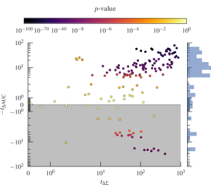
Figure 3: Significance of the discrepancy between model selection approaches. For each pair of model classes and for all of the empirical networks in table 1, we show the t-statistic (Eq. 14) for the difference in AUC and the description length $\Sigma$. Results correspond to 30-150 edge removal experiments of a fraction $f=0.05$ of the edges (we observe similar results for different fractions of removed edges). The number of repetitions for each network is different because for larger networks it takes a longer time to get the results but, at the same time, the fluctuations between results are smaller. In general, we use as many repetitions as necessary to get reasonable error bars in all our estimates. Colors (gray tones) show the associated $p$-value. Points in the top-half of the figure indicate a consistency between both model selection criteria: The model with the smallest description length also yields the largest AUC. For points in the bottom-half (grey), the comparisons are inconsistent. On the right axis, we show a histogram of the $t_{\Delta\text{AUC}}$ values, showing that a majority of comparisons are consistent.

To quantify how frequent such discrepancies are, we systematically compare the compressiveness and the predictive power of all model classes on all networks (Fig. 3). For each network and each model class, we generate a noisy observation $\bm{A^{O}}$ by removing a fraction $f=0.05$ of the links and obtain the optimal partition $\bm{b}=\bm{b}^{*}$ as in Eq. 13. We use this optimal partition to compute the description length $\Sigma(\bm{b}^{*},\mathcal{C})$ and the AUC for the prediction of the missing links. We repeat this operation 30 to 150 times for each real network, and for each set of missing edges and each pair of models we compute the difference in description length and AUC, $\Delta\Sigma$ and $\Delta\text{AUC}$. For each model pair, we have a population of such values, which we use to compute the $t$-statistic for a null model with zero mean, e.g. for $\Delta\Sigma$ we have

$$t_{\Delta\Sigma}=\frac{{\left<\Delta\Sigma\right>}}{\sigma_{\Delta\Sigma}/\sqrt{n}},$$ (14)

where ${\left<\Delta\Sigma\right>}$, $\sigma_{\Delta\Sigma}$ and $n$ are the mean, standard deviation and size of the population; and analogously for $t_{\Delta\text{AUC}}$. With a value of $t_{\Delta\Sigma/\Delta\text{AUC}}$ and the sample size, we can obtain the associated $p$-value, from which the null hypothesis can be rejected if it is sufficiently small.

Figure 3 shows the results from model class comparisons for all datasets in table 1. Note that while the majority of comparisons (81%) are consistent, we observe a non-negligible fraction of significantly inconsistent comparisons (19%). Taking into account the synthetic example from the previous section, the observed fraction of inconsistent comparisons should not come as a surprise. Nevertheless, we do not claim that the reason for the discrepancies observed in the empirical data is precisely the same as the one in the planted partition example.

Dataset	$N$	${\left<k\right>}$
American college football Girvan and Newman (2002)	$115$	$10.7$
Florida food web (dry) Ulanowicz and DeAngelis (2005)	$128$	$33.4$
Residence hall friendships Freeman et al. (1998)	$217$	$24.6$
C. elegans neural network White et al. (1986)	$297$	$15.9$
Scientific coauthorships Newman (2006)	$379$	$4.8$
E-mail Guimerà et al. (2003)	$1,133$	$9.6$
Political blogs Adamic and Glance (2005)	$1,222$	$31.2$
Crimes in St. Louis Kunegis (2013)	$1,380$	$2.13$
Protein iteractions (I) Stelzl et al. (2005)	$1,706$	$7.3$
Bible name co-ocurrences Kunegis (2013)	$1,773$	$10.3$
Hamsterster friendships Kunegis (2013)	$1,858$	$13.5$
Movielens ratings Kunegis (2013)	$2,625$	$75.2$
Adolescent friendships Moody (2001)	$2,539$	$10.2$
Global airport network Peixoto (2014)	$3,286$	$41.6$
Protein iteractions (II) Joshi-Tope et al. (2005)	$6,327$	$46.6$
Internet AS Leskovec et al. (2007)	$6,474$	$4.3$
Advogato user trust Massa et al. (2009)	$6,541$	$15.6$
Cora citations Šubelj and Bajec (2013)	$23,166$	$7.9$
DBLP citations Ley (2002)	$12,591$	$7.9$
Google+ social network Leskovec and Mcauley (2012)	$23,628$	$3.3$
arXiv hep-th citations Leskovec et al. (2007)	$27,770$	$25.4$
Digg online converstations Choudhury et al. (2009)	$30,398$	$5.77$
Linux source dependency Kunegis (2013)	$30,837$	$13.9$
PGP web of trust Richters and Peixoto (2011)	$39,796$	$15.2$
Facebook wall posts Viswanath et al. (2009)	$46,952$	$37.4$

Table 1: Empirical networks used in this work, with their number of nodes $N$ and average degree ${\left<k\right>}=2E/N$.

IV.3 Ensembles of simple models are more predictive than the single most compressive model

We have shown that the model that best performs at link prediction is often the most likely one or, equivalently, the one that best compresses the data. Importantly, even for the cases in which both model selection approaches are consistent, the single most compressive does not necessarily provide optimal link predictions.

Indeed, according to Eq. 11, the best approximation to the probability of a link is given by the average over all partitions in a model class Hoeting et al. (1999). Although this average cannot be calculated exactly because of the combinatorially large number of partitions, one can use Markov chain Monte Carlo (MCMC) to sample over the partitions with the appropriate posterior distribution $P(\bm{b}|\bm{A^{O}},\mathcal{C})$ Guimerà and Sales-Pardo (2009). Then, the average over all partitions is approximated by the average over the sampled partitions, which asymptotically coincides with the exact value.

Note that if the posterior is dominated by a single partition (that is, if the model is a perfect fit to the data) the single-point estimate Eq. III.2 will be an excellent approximation to the average and these two approaches will coincide. However, when the model is not a perfect fit, either due to lack of statistical evidence, or more realistically, due to an imperfect description of the true underlying generative mechanism, they will not.

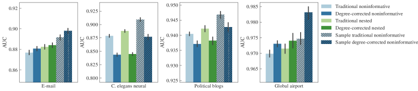
Figure 4: Comparison between single-point and average link prediction for four real networks and the four model classes. Single-point predictions are obtained using Eq. III.2 whereas average predictions are obtained using MCMC sampling to approximate Eq. 11. In all cases, we removed a fraction $f=0.05$ of the true links of the network, and computed the AUC to measure predictive power (see text). Sampling with the simplest model class (the traditional non-informative SBM) always gives more accurate predictions than the single-point prediction with the best model.

For some of the networks in Table I, we have compared the predictive power of single-point estimates with the four model classes, and compared them to the predictive power of averages obtained using MCMC sampling on the model classes with non-informative priors. Fig. 4 shows that averaging over many partitions improves the capacity of predicting missing edges, indicating that the data is not perfectly described by the best partition. Interestingly, the difference in AUC scores is often larger between the best partition and the model average than it is across model classes. This indicates that in-class variability is often more expressive of the data (at least with respect to predictive performance) than the single best fit of the most compressive model class. Nevertheless, we still observe that the most compressive model class also tends to yield higher predictive performance when averaged over partitions.

V Conclusion

We have compared two approaches to model selection, one based on maximum posterior likelihood (or maximum compression), and another based on maximum performance at missing link prediction. We have found that while these criteria tend to agree in practice, they fail to give consistent results in some cases. In particular, we have seen that link prediction can lead to overfitting because, perhaps counter-intuitively, overly complex models sometimes give better predictions.

The fact that data prediction (in particular leave-one-out cross validation) does not yield a consistent estimator of the underlying generative process is well understood for linear models Shao (1993), which is the same problem we have observed for the SBM when only one link is removed. However, it was also shown in Ref. Shao (1993) that cross validation for linear models is consistent if one performs leave-$k$-out, with $k$ scaling proportionally with the number of data points in the training set. However, doing so when the total amount of data is fixed, means we must leave a large amount of data out of the inference procedure, incurring a substantial loss of precision. We are thus left with two competing goals: Increase the training set to maximize inference precision, and increase the validation set to guarantee consistency. Both can be achieved simultaneously only when the data is plentiful, and when the model is well specified — conditions that cannot be always guaranteed in practice. For networks, even under the SBM assumption, there are currently no good recipes to reach the proper balance, or an assurance that such a balance even exists. This problem is particularly exacerbated by the fact that most networks are sparse, and hence there might be insufficient data to confidently identify the correct model even when they are infinitely large. In fact, a removal of a fraction of edges will always make the network sparser, potentially crossing a threshold that makes the latent structure completely undetectable Decelle et al. (2011).

An important ramification of our results is that the potential overfitting that can arise out of seeking the best predictions does not mean that one should avoid doing it altogether. On the contrary, overfitting becomes a non-issue if the main objective is to generalize from previous observations and guess possible errors and omissions in the data, or predict future observations, with the highest precision. In this situation we have shown that the best approach is, in fact, to average over models, rather than use a single model. In any case, one should always be careful not to conclude that the preferred model or models in this situation are closer to the actual underlying generative process.

Appendix A Posterior probability of missing links and non-links

Our goal is to obtain an expression for the posterior likelihood of missing entries $P(\delta\bm{A}|\bm{A^{O}})$, conditioned on the observed network $\bm{A^{O}}$. We will make use of only two simple assumptions about the data-generating process. First, we assume that the complete network $\bm{G}=\bm{A^{O}}\cup\delta\bm{A}$ is sampled from some version of the SBM with a marginal likelihood

$$P_{G}(\bm{G}|\bm{b})=P(\bm{G}|\bm{b},\mathcal{C}).$$

Secondly, given a generated network $\bm{G}$, we then select a portion of the entries $\delta\bm{A}$ from some distribution,

$$P_{\delta A}(\delta\bm{A}|\bm{G}),$$ (15)

which models our source of errors. The observed network is obtained from the above construction by removing $\delta\bm{A}$ from $\bm{G}$,

$$\bm{A^{O}}=\bm{G}\setminus\delta\bm{A},$$ (16)

where the notation above means that the edges and non-edges present in $\delta\bm{A}$ and $\bm{G}$ are left indeterminate in $\bm{A^{O}}$ (although, e.g. considering edges them as non-edges in $\bm{A^{O}}$, i.e. $\bm{A^{O}}=\bm{G}-\delta\bm{A}$ would yield an identical outcome, as we show below). Given the above model, we want to write down the joint likelihood $P(\bm{A^{O}},\delta\bm{A}|\bm{b})$, so that we can obtain the conditional likelihood $P(\delta\bm{A}|\bm{A^{O}},\bm{b})$. We begin by using Eq. 16 to write

$$P(\bm{A^{O}}|\delta\bm{A},\bm{G}) =\delta(\bm{A^{O}}-(\bm{G}\setminus\delta\bm{A})),$$

$$=\delta(\bm{G}-(\bm{A^{O}}\cup\delta\bm{A})),$$

since there is only one possibility which is consistent, where $\delta(\bm{B}-\bm{C})=1$ if $\bm{B}=\bm{C}$ or $0$ otherwise. Thus, if we know the complete graph $\bm{G}$, we can write the joint likelihood as

$$P(\bm{A^{O}},\delta\bm{A}|\bm{G}) =P(\bm{A^{O}}|\delta\bm{A},\bm{G})P_{\delta A}(\delta\bm{A}|\bm{G}),$$

$$=\delta(\bm{G}-(\bm{A^{O}}\cup\delta\bm{A}))P_{\delta A}(\delta\bm{A}|\bm{G}).$$

Finally, for the joint distribution conditioned on the partition, we sum the above over all possible graphs $\bm{G}$, sampled from our original model,

$$P(\bm{A^{O}},\delta\bm{A}|\bm{b}) =\sum_{\bm{G}}P(\bm{A^{O}},\delta\bm{A}|\bm{G})P_{G}(\bm{G}|\bm{b})$$

$$=P_{\delta A}(\delta\bm{A}|\bm{A^{O}}\cup\delta\bm{A})P_{G}(\bm{A^{O}}\cup\delta\bm{A}|\bm{b}).$$

From this, we can write directly our desired posterior of missing entries by averaging over all possible partitions,

$$P(\delta\bm{A}|\bm{A^{O}}) =\frac{\sum_{\bm{b}}P(\bm{A^{O}},\delta\bm{A}|\bm{b})P(\bm{b})}{P(\bm{A^{O}})}$$ (17)

$$=\frac{P_{\delta A}(\delta\bm{A}|\bm{A^{O}}\cup\delta\bm{A})\sum_{\bm{b}}P_{G}(\bm{A^{O}}\cup\delta\bm{A}|\bm{b})P(\bm{b})}{P(\bm{A^{O}})},$$ (18)

with $P(\bm{A^{O}})$ being a normalization constant, independent of $\delta\bm{A}$. Note that the equation above does not depend on whether $\bm{A^{O}}$ includes the missing entries as edges or non-edges, or if they are left indeterminate as we have, as the only relevant quantity in the numerator is the complete graph $\bm{A^{O}}\cup\delta\bm{A}$. Therefore, even though these representations amount to very different interpretations of the data, they result in the same inference outcome, since in the end all that matters is the model we have for the complete network.

Although it is complete, Eq. 18 cannot be used directly to compute posterior likelihood, as it includes a sum over all partitions. It does, however, suggest a simple algorithm: We could compute the average of $P_{G}(\bm{A^{O}}\cup\delta\bm{A}|\bm{b})$ by sampling many partitions $\bm{b}$ from the prior $P(\bm{b})$. However, even though it is correct, this algorithm will typically take an astronomical time to converge to the asymptotic value, since the largest values of $P_{G}(\bm{A^{O}}\cup\delta\bm{A}|\bm{b})$ will be far away from the typical values of $\bm{b}$ sampled from $P(\bm{b})$. Instead, a much better algorithm is obtained by performing importance sampling, i.e. by writing the likelihood as

$$P(\delta\bm{A}|\bm{A^{O}}) \propto P_{\delta A}(\delta\bm{A}|\bm{A^{O}}\cup\delta\bm{A})\sum_{\bm{b}}P_{G}(\bm{A^{O}}\cup\delta\bm{A}|\bm{b})\frac{P_{G}(\bm{A^{O}}|\bm{b})}{P_{G}(\bm{A^{O}}|\bm{b})}P(\bm{b}),$$

$$\propto P_{\delta A}(\delta\bm{A}|\bm{A^{O}}\cup\delta\bm{A})\sum_{\bm{b}}\frac{P_{G}(\bm{A^{O}}\cup\delta\bm{A}|\bm{b})}{P_{G}(\bm{A^{O}}|\bm{b})}P_{G}(\bm{b}|\bm{A^{O}}).$$ (19)

where we have used

$$P_{G}(\bm{b}|\bm{A^{O}})=\frac{P_{G}(\bm{A^{O}}|\bm{b})P(\bm{b})}{P_{G}(\bm{A^{O}})},$$

which is the posterior of $\bm{b}$ pretending that $\bm{A^{O}}$ came directly from the SBM, which we can sample efficiently using MCMC. Naturally, if the number of entries in $\delta\bm{A}$ is much smaller than in $\bm{A^{O}}$, this posterior distribution will be much closer to the region of interest, and the estimation of the likelihood will converge significantly faster. Note, however, that in order to compute $P_{G}(\bm{A^{O}}|\bm{b})$ and sample from $P_{G}(\bm{b}|\bm{A^{O}})$ we must decide whether the missing edges/non-edges in $\bm{A^{O}}$ are really missing or if we replace them with zeros or ones. The choice, however, cannot change the resulting distribution $P(\delta\bm{A}|\bm{A^{O}})$, as it is invariant with respect to the weights we use when doing importance sampling. Hence, the choice we make should done purely on algorithmic grounds. In our experiments we will consider missing edges (non-edges) as non-edges (edges), since it allows MCMC implementations developed for this case to be used without modification.

To complete the estimation, we need to define how the edges and non-edges are removed from the original network. Without loss of generality, focusing on the case of missing edges only, a simple assumption is a uniform distribution conditioned on the fraction of missing edges $f$,

$$P_{\delta A}(\delta\bm{A}|\bm{G},f) =\prod_{i<j}{G_{ij}\choose\delta A_{ij}}f^{\delta A_{ij}}(1-f)^{G_{ij}-\delta A_{ij}}$$

$$=f^{E_{\delta}}(1-f)^{E_{G}-E_{\delta}},$$ (20)

where $E_{\delta}$ and $E_{G}$ are the total number of edges that are removed and in the original network, respectively, and we have assumed a simple graph in the last equation for simplicity. If we are always considering the same number of missing edges, Eq. A is only a constant, resulting in

$$P(\delta\bm{A}|\bm{A^{O}})\propto\sum_{\bm{b}}\frac{P_{G}(\bm{A^{O}}\cup\delta\bm{A}|\bm{b})}{P_{G}(\bm{A^{O}}|\bm{b})}P_{G}(\bm{b}|\bm{A^{O}}).$$ (21)

which is Eq. 11 in the main text. This equation is exact up to a normalization constant that is often unnecessary to compute, as we are mostly interest in relative probabilities of missing edges. We stress that in deriving Eq. 21 we have not made any reference to the internal structure of the network model $P_{G}(\bm{G}|\bm{b})$, and is equally valid not only for all model variants used in this work, but also to a much wider class. This is in contrast to similar frameworks that have been derived with much more specific models in mind Clauset et al. (2008); Guimerà and Sales-Pardo (2009). Furthermore, we note also that although we have assumed in the last steps that $\delta\bm{A}$ is a set of missing edges, the same argument above can be adapted with almost no changes when it represents instead any arbitrary combination of missing and spurious edges, and hence our framework can be used in this more general scenario as well.

We note that the problem of selecting the most appropriate fraction of missing edges with the objective of performing model selection is not a trivial one. In fact, only creating missing edges but not spurious ones is a biased way to proceed, since a more accurate representation of the data would consider edges and non-edges on equal footing. However, choosing the optimal relative fraction would require not only preserving the sparsity of the data (i.e. selecting a larger fraction of missing edges than spurious ones) but also more information about the heterogeneous mixture of edge populations, which would depend on the true model parameters. We leave this open problem for a future work, and concentrate instead of the more typical task of missing edge prediction.

Appendix B Link prediction is not always a good model selection criterion: The planted partition example

\begin{overpic}[width=143.09538pt]{{pp-best-auc_bayes-mdl-nr100-B10-ak20-f0.0}.pdf} \put(0.0,10.0){(a)} \end{overpic}

\begin{overpic}[width=143.09538pt]{{pp-best-auc_bayes-mdl-nr100-B10-ak20-f0.05}.pdf} \put(0.0,10.0){(b)} \end{overpic}

\begin{overpic}[width=143.09538pt]{{pp-best-ddl-mdl-nr100-B10-ak20-f0.0}.pdf} \put(0.0,10.0){(c)} \end{overpic}

Figure 5: (a) Average AUC values obtained by removals of a single edge from a PP with $n_{r}=100$, $B=10$ and ${\left<k\right>}=20$, both for “canonical” (i.e. unconstrained) as well as microcanonical samples, where Eq. 23 holds. The legend indicates which model was used to compute the AUC (i.e. the SBM or the DC-SBM). The solid line corresponds to Eq. 34, and the vertical line the value $c^{*}=1/B+(B-1)/(B\sqrt{{\left<k\right>}})$ corresponding to the detectability threshold. The inset shows the difference of the AUC values obtained with the two model classes, $\text{AUC}_{\text{DC-SBM}}-\text{AUC}_{\text{SBM}}$, with networks sampled from the canonical model. (b) The same as (a), but with a fraction $f=0.05$ of the edges removed. (c) Description length difference between the SBM and DC-SBM, both for the canonical and microcanonical samples, for a fraction $f=0.05$ of the edges removed.

\begin{overpic}[width=106.23808pt]{{pp-best-auc_bayes-mdl-Bfit-canonicalFalse-deg_corrFalse-c0.7923076923076923-nr100-B10-ak20-f0.05}.pdf} \put(0.0,10.0){(a)} \end{overpic}

\begin{overpic}[width=106.23808pt]{{pp-best-dl-mdl-Bfit-canonicalFalse-deg_corrFalse-c0.7923076923076923-nr100-B10-ak20-f0.05}.pdf} \put(0.0,10.0){(b)} \end{overpic}

Figure 6: (a) AUC values obtained by removing a fraction $f=0.05$ of the edges of a PP with $n_{r}=100$, $B=10$, ${\left<k\right>}=20$ and $c=0.8$, for microcanonical samples fulfilling Eq. 23, and forcing $B=B^{\prime}$ during inference. (b) The same as (a), but with the description length $\Sigma$, instead. The MDL criterion pinpoints the correct planted value of $B^{\prime}=10$, whereas AUC overfits.

We consider a simple parametrization of the non-degree-corrected SBM known as the planted-partition model (PP), which is composed of $N$ nodes divided into $B$ equal-sized groups and is generated according to Eq. 3 with

$$\lambda_{rs}=\frac{2{\left<E\right>}}{n_{r}n_{s}}\left[\frac{c\delta_{rs}}{B}+\frac{(1-c)(1-\delta_{rs})}{B(B-1)}\right],$$ (22)

where $n_{r}=N/B$, ${\left<E\right>}$ is the average number of edges, and $c\in[0,1]$ controls the degree of assortativity between groups. For $c>1/B$ the placement of edges is not fully random, and for $c>1/B+(B-1)/(B\sqrt{{\left<k\right>}})$ the planted modular structure is detectable from the data alone Decelle et al. (2011). In the following discussion we assume that $c>1/B$ and that the partition of the nodes is always known a priori.

Specifically, we consider networks which have an observed number of edges between groups that matches exactly the expected value,

$$e_{rs}=\sum_{ij}A_{ij}\delta_{b_{i}r}\delta_{b_{i}s}=\lfloor n_{r}n_{s}\lambda_{rs}\rceil,$$ (23)

where $\lfloor x\rceil$ rounds $x$ to the nearest integer.

When faced with an instance of this model, we want to evaluate the predictiveness of the model by performing leave-one-out cross validation: We remove a single edge from the network, and consider its likelihood according to the observed network. Based on this we compute the AUC, i.e. the probability that the removed edge is ranked above the false positives. Here we show how the result of this experiment can be computed analytically.

We begin by considering a slightly different scenario: Instead of computing the likelihood of the missing edge via the posterior distribution, we use instead the true likelihood of the original model, before we removed the edge. When doing so, because of the symmetries in the model, there will be only two possible values of the likelihood, depending only on whether the removed edge lies between nodes of the same or different groups. If the removed edge connects nodes of the same group, the only false positives that have the same likelihood will be those that also connect nodes of the same group (although they do not need to be the same group of the removed edge), and the remaining edges will have a lower likelihood. With this, and assuming that $N\gg 1$ and sufficiently sparse networks so that $e_{rs}<n_{r}n_{s}$, the computed AUC will be

$$\text{AUC}_{\text{in}} =\frac{1}{N^{2}/2}\left[\frac{1}{2}\frac{Bn_{r}^{2}}{2}+\frac{B(B-1)}{2}n_{r}^{2}\right]$$ (24)

$$=\frac{1}{2B}+\frac{(B-1)}{B},$$ (25)

which means we have $\text{AUC}_{\text{in}}>1/2$ if $B>1$, indicating that we can predict the missing edge better than pure chance. For removed edges between different groups, we have instead,

$$\text{AUC}_{\text{out}} =\frac{1}{N^{2}/2}\frac{1}{2}\frac{B(B-1)}{2}n_{r}^{2}$$ (26)

$$=\frac{(B-1)}{2B},$$ (27)

from which we see that $\text{AUC}_{\text{out}}<1/2$, i.e. edges between groups are predicted with a performance that is inferior to fully random guesses. Overall, the average performance for randomly chosen edges is

AUC $$=c\text{AUC}_{\text{in}}+(1-c)\text{AUC}_{\text{out}}$$ (28)

$$=c\left[\frac{1}{2B}+\frac{(B-1)}{2B}\right]+\frac{B-1}{2B}.$$ (29)

For any $c>1/B$ we have that $\text{AUC}>1/2$, meaning that the generative model on average provides better predictions of randomly missing edges that are better than pure chance. This behavior is fully expected, since the process generating the missing edges is not random, and is described precisely by our model.

However, in the scenario of an actual missing link, we need to infer the model from the observed data, in the absence of the removed edge. If the removed edge connects groups $r$ and $s$, the new edge counts between these two groups will be $(e_{rs}-1-\delta_{rs})$, and hence the posterior likelihood of observing a missing link there will be slightly smaller than in the true model. Since in the original model all other edges of the same kind (inter or intra-group) had exactly the same likelihood, this small difference in the likelihood will be sufficient to make the actual missing edge less likely than all the other ones with the same likelihood originally. Because of this, in this situation we have

$$\text{AUC}_{\text{in}} =\frac{1}{N^{2}/2}\left[\frac{1}{2}\frac{n_{r}^{2}}{2}+\frac{B(B-1)}{2}n_{r}^{2}\right]$$ (30)

$$=\frac{1}{2B^{2}}+\frac{(B-1)}{B},$$ (31)

and

$$\text{AUC}_{\text{out}} =\frac{1}{N^{2}/2}\frac{1}{2}n_{r}^{2}$$ (32)

$$=\frac{1}{2B^{2}},$$ (33)

and thus

AUC $$=c\text{AUC}_{\text{in}}+(1-c)\text{AUC}_{\text{out}}$$ (34)

$$=\frac{1}{2B^{2}}+c\frac{B-1}{B}.$$ (35)

Differently from the case where the true model is known, now if $1/B<c<(B^{2}-1)/[2B(B-1)]$ we have a non-random inferred model that yields $\text{AUC}<1/2$, and thus an inferior predictive performance than pure chance, despite the fact that the model differs from the true one only minimally. The reason for this is that the removal of any single edge decreases its probability — according to the model inferred from the remaining network — below a vast number of false positives (i.e. edges of the same kind), which in fact have the exact same likelihood under the original model.

As mentioned in the main text, if we infer using the wrong model class, for example the DC-SBM, we systematically observe larger AUC values, as can be seen in Fig. 5a. This is because the extra parameters of this model — the degree propensities $\theta_{i}$ — incorporate a large amount of noise from the data and destroy the homogeneity present in the simpler model. Without the homogeneity, the single edge count lost between groups $r$ and $s$ makes little difference overall. As can also be seen in Fig. 5b, this phenomenon persists even if we remove a finite fraction of the edges, instead of a single one.

Despite the improved predictive performance, the DC-SBM is not the most appropriate model for this network. Not only we generated the data explicitly from the simpler SBM, but also its posterior likelihood is smaller, as reflected by its larger description length (see Fig. 5c). Hence, the unsupervised model selection approach is impervious to details of the model such as the fact that the edge probabilities are similar, and correctly identifies the true generative process. We emphasize that even if one would stubbornly prefer the most predictive model in this case, one would have to accept a fully random network over the simpler SBM, when the later yields AUC values smaller than 1/2.

The reason why link prediction fails to select the true underlying model in this case is not the lack of statistical evidence, but rather that the model itself — and not the data — is sensitive to perturbations: A minimal change to one of the $\lambda_{rs}$ values downgrades or upgrades the likelihood of the respective edges with respect to all others of different types that would otherwise have the exact same probability. Hence, this example illustrates how in some cases predictive performance (at least when measured by the AUC) can be to some extent an inherent property of a model, regardless of its quality of fit to the data.

One could argue that although the networks that obey Eq. 23 have the largest probability, they are nevertheless not representative of the whole ensemble: Since the edge counts $e_{rs}$ are sums of Poisson variables, they are also distributed according to a Poisson, and therefore their probabilities of matching exactly the expected values will decrease as $P(e_{rs}=n_{r}n_{s}\lambda_{rs})\approx 1/\sqrt{n_{r}n_{s}\lambda_{rs}}$, for large arguments. For large and sparse networks, this value will decrease as $1/\sqrt{N}$, and hence, despite being the most likely type of network, its absolute probability will be very small asymptotically, and therefore most networks sampled from this model will not possess such an extreme level of homogeneity. Because of this, one could say that this is an “out-of-class” example, and that would perhaps explain the inconsistency. Although this is technically true, it is easy to see that this argument is a red herring: We can easily view the above case as a typical instance of an equivalent microcanonical model Peixoto (2017), where the homogeneity of Eq. 23 is strictly imposed for all sampled networks, and the rest of the analysis would still remain valid. Nevertheless, we can also show that the same problem occurs for typical samples from the original ensemble, which do not necessarily conform to Eq. 23, albeit less prominently. As seen in the inset of Fig. 5b, for a range of the parameter $c$ — in particular when the structure of the model is strongest — we still observe higher AUC values for the DC-SBM, at least when the fraction of removed edges is sufficiently large. The explanation we offer is the same: the fluctuations are not always sufficient to mask the homogeneity in the true model, which thwarts the predictability of missing edges.

The above phenomenon also interferes with the selection of the number of groups. Link prediction has been proposed before as a means of selecting the number of groups Kawamoto and Kabashima (2016), as well as other dimensional aspects De Bacco et al. (2017), but as we show in Fig. 6 it also fails for precisely the same reason: increasing the number of groups incorporates more noise in the model, and breaks its homogeneity. This leads to a clear overfitting, where spurious groups are identified. As before, unsupervised model selection is not susceptible to this, and reliably selects the correct number of groups. Because of this possibility, we admonish against using the supervised approach in favor of the unsupervised for this purpose.