Kinodynamic Planning on Constraint Manifolds

Abstract

This paper presents a motion planner for systems subject to kinematic and dynamic constraints. The former appear when kinematic loops are present in the system, such as in parallel manipulators, in robots that cooperate to achieve a given task, or in situations involving contacts with the environment. The latter are necessary to obtain realistic trajectories, taking into account the forces acting on the system. The kinematic constraints make the state space become an implicitly-defined manifold, which complicates the application of common motion planning techniques. To address this issue, the planner constructs an atlas of the state space manifold incrementally, and uses this atlas both to generate random states and to dynamically simulate the steering of the system towards such states. The resulting tools are then exploited to construct a rapidly-exploring random tree (RRT) over the state space. To the best of our knowledge, this is the first randomized kinodynamic planner for implicitly-defined state spaces. The test cases presented in this paper validate the approach in significantly-complex systems.

I Introduction

The motion planning problem has been a subject of active research since the early days of Robotics [33]. Although it can be formalized in simple terms—find a feasible trajectory to move a robot between two states—and despite the significant advances in the field, it is still an open problem in many respects. The complexity of the problem arises from the multiple constraints that have to be taken into account, such as potential collisions with static or moving objects in the environment, kinematic loop-closure constraints, torque and velocity limits, or energy and time execution bounds, to name a few. All these constraints are relevant in the factory and home environments in which Robotics is called to play a fundamental role in the near future.

The complexity of the problem is typically tackled by first relaxing some of the constraints. For example, while obstacle avoidance is a fundamental issue, the lazy approaches initially disregard it [9]. Other approaches concentrate on geometric [31] and kinematic feasibility [26] from the outset, which constitute already challenging issues by themselves. In these and other approaches [20], dynamic constraints such as speed, acceleration, or torque limits are neglected, with the hope that they will be enforced in a postprocessing stage. Decoupled approaches, however, may not lead to solutions satisfying all the constraints. It is not difficult to find situations in which a kinematically-feasible, collision-free trajectory becomes unusable because it does not account for the system dynamics (Fig. 1).

[width=.8]fig1

Figure 1: A kindoynamic planning problem on a four-bar pendulum modeling a swing boat ride. Top: The start and goal states, both with null velocity. Bottom: The kinematic constraints define an helicoidal manifold. A kinematically-feasible trajectory (red) and a trajectory also fulfilling dynamic constraints (green) may be quite different.

This paper presents a sampling-based planner that simultaneously considers collision avoidance, kinematic, and dynamic constraints. The planner constructs a bidirectional rapidly-exploring random tree (RRT) on the state space manifold implicitly defined by the kinematic constraints. In the literature, the suggested way to define an RRT including such constraints is to differentiate them and add them to the ordinary differential equations (ODE) defined by the dynamic constraints [35]. In such an approach, however, the underlying geometry of the problem would be lost. The random samples used to guide the RRT extension would not be generated on the state space manifold, but in the larger ambient space, which results in inefficiencies [26]. The numerical integration of the resulting ODE system, moreover, would be affected by drift (Fig. 2). In some applications, such a drift might be tolerated, but in others, such as in robots with closed kinematic loops, it would render the simulation unprofitable due to unwanted link penetrations, disassemblies, or contact losses. In this paper, the sampling and drift issues are addressed by preserving the underlying geometry of the problem. To this end, we propose to combine the extension of the RRT with the incremental construction of an atlas of the state space manifold [37]. The atlas is enlarged as the RRT branches reach yet unexplored areas of the manifold. Moreover, it is used to effectively generate random states and to dynamically simulate the steering of the system towards such states.

[width=]torus

Figure 2: Drift caused by numerical integration of an ODE system. Top: A particle moving on a torus under the shown vector field. The trajectory obtained by the forward Euler method (red) increasingly diverges from the exact trajectory (yellow). Bottom: With more accurate procedures, such as the 4th order Runge-Kutta method (blue), the drift may be reduced, but not canceled.

This paper is organized as follows. Section II puts the proposed planner in the context of existing approaches. Section III formalizes the problem and paves the way to Section IV, which describes the fundamental tools to map and explore an implicitly-defined state space. The resulting planner is described in Section V and experimentally validated in Section VI. Finally, Section VII concludes the paper and discusses points deserving further attention.

II Related Work

The problem of planning under dynamic constraints, also known as kinodynamic planning [35], is harder than planning with geometric constraints, which is already known to be PSPACE-hard [48, 13]. Although particular, exact solutions for some systems have been given [19], general solutions do also exist. Dynamic programming approaches, for example, define a grid of cost-to-go values to search for a solution [1, 39, 17], and can compute accurate solutions in lower-dimensional problems. Such an approach, however, does not scale well to problems with many degrees of freedom. In contrast, numerical optimization techniques [29, 46, 49, 54, 5] can be applied to remarkably-complex problems, although they may not converge to feasible solutions. A widely used alternative is to rely on sampling-based approaches [18, 35]. These methods can cope with high-dimensional problems, and guarantee to find a feasible solution, if it exists and enough computing time is available. The RRT method [36] stands out among them, due to its effectiveness and conceptual simplicity. However, it is well known that RRT planners can be inefficient in certain scenarios [14]. Part of the complexity arises from planning in the state space instead of in the lower-dimensional configuration space [42]. Nevertheless, the main issue of RRT approaches is the disagreement of the metric used to measure the distance between two given states, and the actual cost of moving between such states, which must comply with the vector fields defined by the dynamic constraints of the system. Several extensions to the basic RRT planner have been proposed to alleviate this issue [52, 32, 43, 50, 30, 15, 16, 27]. None of these extensions, however, can deal with the implicitly-defined configuration spaces that arise when the problem includes kinematic constraints [51, 4, 44, 26]. When considering both kinematic and dynamic constraints, the planning problem requires the solution of differential algebraic equations (DAE). The algebraic equations derive from the kinematic constraints and the differential ones reflect the system dynamics.

From constrained multibody dynamics it is well known that, when simulating a system’s motion, it is advantageous to directly deal with the DAE of the system, rather than converting it into its ODE form [41]. Several techniques have been used to this end [2, 34]. In the popular Baumgarte method the drift is alleviated with control techniques [3], but the control parameters are problem dependent and there is no general method to tune them. Another way to reduce the drift is to use violation suppression techniques [11, 6], but they do not guarantee a drift-free integration. A better alternative are the methods relying on local parameterizations [47], since they cancel the drift to machine accuracy. To the best of our knowledge, this approach has never been applied in the context of kinodynamic planning. However, it nicely complements an existing planning method for implicitly-defined configuration spaces [44, 26], which also relies on local parameterizations. The planner introduced in this paper can be seen as an extension of the latter method to also deal with dynamics, or an extension of [36] to include kinematic constraints.

III Problem formalization

A robot configuration is described by means of a tuple $q$ of $n_{q}$ generalized coordinates $q_{1},\ldots,q_{n_{q}}$, which determine the positions and orientations of all links at a given instant of time. There is total freedom in choosing the form and dimension of $q$, but it must describe one, and only one, configuration. In this paper we restrict our attention to constrained robots, i.e., those in which $q$ must satisfy a system of $n_{e}$ nonlinear equations

$${\mbox{\bm{$\Phi$}}}({\mbox{\bm{$q$}}})={\mbox{\bm{$0$}}},$$ (1)

which express all joint assembly, geometric, or contact constraints to be taken into account, either inherent to the robot design or necessary for task execution. The configuration space $\mathcal{C}$ of the robot, or C-space for short, is the nonlinear variety

$$\mathcal{C}=\{{\mbox{\bm{$q$}}}:{\mbox{\bm{$\Phi$}}}({\mbox{\bm{$q$}}})={\mbox{\bm{$0$}}}\},$$

which may be quite complex in general. Under mild conditions, however, we can assume that the Jacobian ${\mbox{\bm{$\Phi$}}}_{{\mbox{\bm{$q$}}}}({\mbox{\bm{$q$}}})$ is full rank for all ${\mbox{\bm{$q$}}}\in\mathcal{C}$, so that $\mathcal{C}$ is a smooth manifold of dimension $d_{\mathcal{C}}=n_{q}-n_{e}$. This assumption is common because C-space singularities can be avoided by judicious mechanical design [8], or through the addition of singularity-avoidance constraints into Eq. (1) [7].

By differentiating Eq. (1) with respect to time we obtain

$${\mbox{\bm{$\Phi$}}}_{{\mbox{\bm{$q$}}}}({\mbox{\bm{$q$}}})\;\dot{{\mbox{\bm{$q$}}}}={\mbox{\bm{$0$}}},$$ (2)

which provides, for a given ${\mbox{\bm{$q$}}}\in\mathcal{C}$, the feasible velocity vectors of the robot.

Let ${\mbox{\bm{$F$}}}({\mbox{\bm{$x$}}})={\mbox{\bm{$0$}}}$ denote the system formed by Eqs. (1) and (2), where ${\mbox{\bm{$x$}}}=({\mbox{\bm{$q$}}},\dot{{\mbox{\bm{$q$}}}})\in\mathbb{R}^{2n_{q}}$. Our planning problem will take place in the state space

$$\mathcal{X}=\{{\mbox{\bm{$x$}}}:{\mbox{\bm{$F$}}}({\mbox{\bm{$x$}}})={\mbox{\bm{$0$}}}\},$$ (3)

which encompasses all possible mechanical states of the robot [35]. The fact that ${\mbox{\bm{$\Phi$}}}_{{\mbox{\bm{$q$}}}}({\mbox{\bm{$q$}}})$ is full rank guarantees that $\mathcal{X}$ is also a smooth manifold, but now of dimension $d_{\mathcal{X}}=2\;d_{\mathcal{C}}$. This implies that the tangent space of $\mathcal{X}$ at $x$,

$$\mathcal{T}_{{\mbox{\bm{$x$}}}}\mathcal{X}=\{\dot{{\mbox{\bm{$x$}}}}\in\mathbb{R}^{2n_{q}}:{\mbox{\bm{$F$}}}_{{\mbox{\bm{$x$}}}}\;\dot{{\mbox{\bm{$x$}}}}={\mbox{\bm{$0$}}}\}$$ (4)

is well-defined and $d_{\mathcal{X}}$-dimensional for any ${\mbox{\bm{$x$}}}\in\mathcal{X}$.

We shall encode the forces and torques of the actuators into an action vector $u$ of dimension $n_{u}$. Our main interest will be on fully-actuated robots, i.e., those for which $n_{u}=d_{\mathcal{C}}$, but the developments that follow are also applicable to over- or under-actuated robots.

Given a starting state ${\mbox{\bm{$x$}}}_{s}\in\mathcal{X}$, and the action vector as a function of time, ${\mbox{\bm{$u$}}}={\mbox{\bm{$u$}}}(t)$, it is well-known that the time evolution of the robot is determined by a DAE of the form

$${\mbox{\bm{$F$}}}({\mbox{\bm{$x$}}})={\mbox{\bm{$0$}}}$$ (5)

$$\dot{{\mbox{\bm{$x$}}}}={\mbox{\bm{$g$}}}({\mbox{\bm{$x$}}},{\mbox{\bm{$u$}}})$$ (6)

The first equation forces the states $x$ to lie in $\mathcal{X}$. The second equation models the dynamics of the system [35], which can be formulated, e.g., using the multiplier form of the Euler-Lagrange equations [47]. For each value of $u$, it defines a vector field over $\mathcal{X}$, which can be used to integrate the robot motion forward in time, using proper numerical methods.

Since in practice the actuator forces are limited, $u$ is always constrained to take values in some bounded subset $\mathcal{U}$ of $\mathbb{R}^{n_{u}}$, which limits the range of possible state velocities $\dot{{\mbox{\bm{$x$}}}}={\mbox{\bm{$g$}}}({\mbox{\bm{$x$}}},{\mbox{\bm{$u$}}})$ at each ${\mbox{\bm{$x$}}}\in\mathcal{X}$. During its motion, moreover, the robot cannot incur in collisions with itself or with the environment, constraining the feasible states $x$ to those lying in a subset $\mathcal{X}_{\text{free}}\subseteq\mathcal{X}$ of non-collision states.

With the previous definitions, the planning problem we confront can be phrased as follows. Given two states of $\mathcal{X}_{\text{free}}$, ${\mbox{\bm{$x$}}}_{s}$ and ${\mbox{\bm{$x$}}}_{g}$, find an action trajectory ${\mbox{\bm{$u$}}}={\mbox{\bm{$u$}}}(t)\in\mathcal{U}$ such that the trajectory ${\mbox{\bm{$x$}}}={\mbox{\bm{$x$}}}(t)$ with ${\mbox{\bm{$x$}}}(0)={\mbox{\bm{$x$}}}_{s}$ of the system determined by Eqs. (5) and (6), fulfills ${\mbox{\bm{$x$}}}(t_{f})={\mbox{\bm{$x$}}}_{g}$ for some time $t_{f}>0$, and ${\mbox{\bm{$x$}}}(t)\in\mathcal{X}_{\text{free}}$ for all $t\in[0,t_{f}]$.

IV Mapping and Exploring the State Space

The fact that $\mathcal{X}$ is an implicitly defined manifold complicates the design of an RRT planner able to solve the previous problem. In general, $\mathcal{X}$ does not admit a global parameterization and there is no straightforward way to sample $\mathcal{X}$ uniformly. The integration of Eq. (6), moreover, will yield robot trajectories drifting away from $\mathcal{X}$ if numerical methods for plain ODE systems are used. Even so, we next see that both issues can be circumvented by using an atlas of $\mathcal{X}$. If built up incrementally, such an atlas will lead to an efficient means of extending an RRT over the state space.

IV-A Atlas construction

Formally, an atlas of $\mathcal{X}$ is a collection of charts mapping $\mathcal{X}$ entirely, where each chart $c$ is a local diffeomorphism ${\mbox{\bm{$\varphi$}}}_{c}$ from an open set $V_{c}\subset\mathcal{X}$ to an open set $P_{c}\subseteq\mathbb{R}^{d_{\mathcal{X}}}$ [Fig. 3(a)]. The $V_{c}$ sets can be thought of as partially-overlapping tiles covering $\mathcal{X}$, in such a way that every ${\mbox{\bm{$x$}}}\in\mathcal{X}$ lies in at least one $V_{c}$. The point ${\mbox{\bm{$y$}}}={\mbox{\bm{$\varphi$}}}_{c}({\mbox{\bm{$x$}}})$ provides the local coordinates, or parameters, of $x$ in chart $c$. Since each ${\mbox{\bm{$\varphi$}}}_{c}$ is a diffeomorphism, its inverse map ${{\mbox{\bm{$\psi$}}}_{c}}={\mbox{\bm{$\varphi$}}}_{c}^{-1}$ exists and gives a local parameterization of $V_{c}$.

To construct ${\mbox{\bm{$\varphi$}}}_{c}$ and ${\mbox{\bm{$\psi$}}}_{c}$ we shall use the so-called tangent space parameterization [47]. In this approach, the map ${\mbox{\bm{$y$}}}={\mbox{\bm{$\varphi$}}}_{c}({\mbox{\bm{$x$}}})$ around a given ${\mbox{\bm{$x$}}}_{c}\in\mathcal{X}$ is obtained by projecting $x$ orthogonally to $\mathcal{T}_{{\mbox{\bm{$x$}}}_{c}}\mathcal{X}$ [Fig. 3(b)]. Thus ${\mbox{\bm{$\varphi$}}}_{c}$ becomes

$${\mbox{\bm{$y$}}}={\mbox{\bm{$U$}}}_{c}^{\!\top}\;({\mbox{\bm{$x$}}}-{\mbox{\bm{$x$}}}_{c}),$$ (7)

where ${\mbox{\bm{$U$}}}_{c}$ is a $2n_{q}\times d_{\mathcal{X}}$ matrix whose columns provide an orthonormal basis of $\mathcal{T}_{{\mbox{\bm{$x$}}}_{c}}\mathcal{X}$. ${\mbox{\bm{$U$}}}_{c}$ can be computed efficiently using the QR decomposition of ${\mbox{\bm{$F$}}}_{{\mbox{\bm{$x$}}}_{c}}$. The inverse map ${\mbox{\bm{$x$}}}={\mbox{\bm{$\psi$}}}_{c}({\mbox{\bm{$y$}}})$ is implicitly determined by the system of nonlinear equations

$$\begin{array}[]{c}{\mbox{\bm{$F$}}}({\mbox{\bm{$x$}}})={\mbox{\bm{$0$}}},\\ {\mbox{\bm{$U$}}}_{c}^{\!\top}({\mbox{\bm{$x$}}}-{\mbox{\bm{$x$}}}_{c})-{\mbox{\bm{$y$}}}={\mbox{\bm{$0$}}}.\end{array}$$ (8)

For a given $y$, these equations can be solved for $x$ by means of the Newton-Raphson method.

[width=0.9]param2manifold2

Figure 3: (a) An atlas is a collection of maps $\varphi$ providing local coordinates to all points of $\mathcal{X}$. The inverse maps $\psi$ convert the vector fields on $\mathcal{X}$ to vector fields on $\mathbb{R}^{d_{\mathcal{X}}}$. (b) The projection of the points ${\mbox{\bm{$x$}}}\in\mathcal{X}$ to $\mathcal{T}_{{\mbox{\bm{$x$}}}_{c}}\mathcal{X}$ leads to specific instances of ${\mbox{\bm{$\varphi$}}}_{c}$ and ${\mbox{\bm{$\psi$}}}_{c}$.

Assuming that an atlas has been created, the problem of sampling $\mathcal{X}$ boils down to sampling the $P_{c}$ sets, since the $y$ values can always be projected to $\mathcal{X}$ using the corresponding map ${\mbox{\bm{$x$}}}={\mbox{\bm{$\psi$}}}_{c}({\mbox{\bm{$y$}}})$. Also, the atlas allows the conversion of the vector field defined by Eq. (6) into one in the coordinate spaces $P_{c}$. The time derivative of Eq. (7), $\dot{{\mbox{\bm{$y$}}}}={\mbox{\bm{$U$}}}_{c}^{\!\top}\dot{{\mbox{\bm{$x$}}}}$, gives the relationship between the two vector fields, and allows writing

$$\dot{{\mbox{\bm{$y$}}}}={\mbox{\bm{$U$}}}_{c}^{\!\top}\>{\mbox{\bm{$g$}}}({\mbox{\bm{$\psi$}}}_{c}({\mbox{\bm{$y$}}}),{\mbox{\bm{$u$}}}),$$ (9)

which is Eq. (6) but expressed in local coordinates. This equation forms the basis of the so-called tangent-space parameterization methods for the integration of DAE systems [22, 23]. Given a state ${\mbox{\bm{$x$}}}_{k}$ and an action $u$, ${\mbox{\bm{$x$}}}_{k+1}$ is estimated by obtaining ${\mbox{\bm{$y$}}}_{k}={\mbox{\bm{$\varphi$}}}_{c}({\mbox{\bm{$x$}}}_{k})$, then computing ${\mbox{\bm{$y$}}}_{k+1}$ using a discrete form of Eq. (9), and finally getting ${\mbox{\bm{$x$}}}_{k+1}={\mbox{\bm{$\psi$}}}_{c}({{\mbox{\bm{$y$}}}_{k+1}})$. The procedure guarantees that ${\mbox{\bm{$x$}}}_{k+1}$ will lie on $\mathcal{X}$, which makes the integration compliant with all kinematic constraints in Eq. (5).

IV-B Incremental atlas and RRT expansion

One could build a full atlas of the implicitly-defined state space [25] and then use its local parameterizations to define a kinodynamic RRT. However, the construction of a complete atlas is only feasible for low-dimensional state spaces. Moreover, only part of the atlas is necessary to solve a given motion planning problem. Thus, a better alternative is to combine the construction of the atlas and the expansion of the RRT [26]. In this approach, a partial atlas is used to generate random states and to add branches to the RRT. Also, as described next, new charts are created as the RRT branches reach unexplored areas of the state space.

Suppose that ${\mbox{\bm{$x$}}}_{k}$ and ${\mbox{\bm{$x$}}}_{k+1}$ are two consecutive steps along an RRT branch whose parameters in the chart defined at ${\mbox{\bm{$x$}}}_{c}$ are ${\mbox{\bm{$y$}}}_{k}$ and ${\mbox{\bm{$y$}}}_{k+1}$, respectively. Then, a new chart at ${\mbox{\bm{$x$}}}_{k}$ is generated if any of the following conditions holds

$$\|{\mbox{\bm{$x$}}}_{k+1}-({\mbox{\bm{$x$}}}_{c}+{\mbox{\bm{$U$}}}_{c}\>{\mbox{\bm{$y$}}}_{k+1})\| >\epsilon,$$ (10)

$$\frac{\|{\mbox{\bm{$y$}}}_{k+1}-{\mbox{\bm{$y$}}}_{k}\|}{\|{\mbox{\bm{$x$}}}_{k+1}-{\mbox{\bm{$x$}}}_{k}\|} <cos(\alpha),$$ (11)

$$\|{\mbox{\bm{$y$}}}_{k+1}\| >\rho,$$ (12)

where $\epsilon$, $\alpha$, and $\rho$ are user-defined parameters. The three conditions are introduced to ensure that the chart domains $P_{c}$ capture the overall shape of $\mathcal{X}$ with sufficient detail. The first condition limits the maximal distance between the tangent space and the manifold. The second condition ensures a bounded curvature in the part of the manifold covered by a local parameterization, as well as a smooth transition between charts. Finally, the third condition is introduced to ensure the generation of new charts as the RRT grows, even for (almost) flat manifolds.

[width=0.9]bounding_box

Figure 4: Bounding of the parameter sets $P_{c}$ and $P_{k}$ of the two neighboring charts in Fig. 3. Note that ${\mbox{\bm{$y$}}}_{c}={\mbox{\bm{$\varphi$}}}_{k}({\mbox{\bm{$x$}}}_{c})$ and ${\mbox{\bm{$y$}}}_{k}={\mbox{\bm{$\varphi$}}}_{c}({\mbox{\bm{$x$}}}_{k})$.

1 Planner(${\mbox{\bm{$x$}}}_{s},{\mbox{\bm{$x$}}}_{g}$)

input : The query states, ${\mbox{\bm{$x$}}}_{s}$ and ${\mbox{\bm{$x$}}}_{g}$.

output : A trajectory connecting ${\mbox{\bm{$x$}}}_{s}$ and ${\mbox{\bm{$x$}}}_{g}$.

2 $T_{s}\leftarrow\textsc{InitRRT}({\mbox{\bm{$x$}}}_{s})$

3 $T_{g}\leftarrow\textsc{InitRRT}({\mbox{\bm{$x$}}}_{g})$

4 $A\leftarrow\textsc{InitAtlas}({\mbox{\bm{$x$}}}_{s},{\mbox{\bm{$x$}}}_{g})$

5 repeat

6       ${\mbox{\bm{$x$}}}_{r}\leftarrow\textsc{Sample}(A,T_{s})$

7       ${\mbox{\bm{$x$}}}_{n}\leftarrow\textsc{NearestState}(T_{s},{\mbox{\bm{$x$}}}_{r})$

8       ${\mbox{\bm{$x$}}}_{l}\leftarrow\textsc{ExtendRRT}(A,T_{s},{\mbox{\bm{$x$}}}_{n},{\mbox{\bm{$x$}}}_{r})$

9       ${\mbox{\bm{$x$}}}_{n}^{\prime}\leftarrow\textsc{NearestState}(T_{g},{\mbox{\bm{$x$}}}_{l})$

10       ${\mbox{\bm{$x$}}}_{l}^{\prime}\leftarrow\textsc{ExtendRRT}(A,T_{g},{\mbox{\bm{$x$}}}_{n}^{\prime},{\mbox{\bm{$x$}}}_{l})$

11       Swap$(T_{s},T_{g})$

12      

13until $\|{\mbox{\bm{$x$}}}_{l}-{\mbox{\bm{$x$}}}_{l}^{\prime}\|<\beta$

Return(Trajectory($T_{s},{\mbox{\bm{$x$}}}_{l},T_{g},{\mbox{\bm{$x$}}}_{l}^{\prime}$))

Algorithm 1 The main procedure of the planner

IV-C Chart coordination

Since the charts will be used to sample the state space uniformly, it is important to reduce the overlap between new charts and those already in the atlas. Otherwise, the areas of $\mathcal{X}$ covered by several charts would be oversampled. To this end, the set of valid parameters for each chart $c$, $P_{c}$, is represented as the intersection of a ball of radius $\rho_{s}$ and a number of half-planes, all defined in $\mathcal{T}_{{\mbox{\bm{$x$}}}_{c}}\mathcal{X}$. The set $P_{c}$ is progressively bounded as new neighboring charts are created around chart $c$. If, while growing an RRT branch using the local parameterization provided by $\mathcal{T}_{{\mbox{\bm{$x$}}}_{c}}\mathcal{X}$, a chart is created on a point ${\mbox{\bm{$x$}}}_{k}$ with parameter vector ${\mbox{\bm{$y$}}}_{k}$ in $P_{c}$, then the following inequality

$${\mbox{\bm{$y$}}}^{\!\top}{\mbox{\bm{$y$}}}_{k}-\frac{\|{\mbox{\bm{$y$}}}_{k}\|^{2}}{2}\leq 0$$ (13)

with ${\mbox{\bm{$y$}}}\in\mathbb{R}^{d_{\mathcal{X}}}$, is added to the definition of $P_{c}$ (Fig. 4). A similar inequality is added to $P_{k}$, the chart at ${\mbox{\bm{$x$}}}_{k}$, by projecting ${\mbox{\bm{$x$}}}_{c}$ to $\mathcal{T}_{{\mbox{\bm{$x$}}}_{k}}\mathcal{X}$. The parameter $\rho_{s}$ must be larger than $\rho$ to guarantee that the RRT branches in chart $c$ will eventually trigger the generation of new charts, i.e., to guarantee that Eq. (12) eventually holds.

1 ExtendRRT($A,T,{\mbox{\bm{$x$}}}_{n},{\mbox{\bm{$x$}}}_{r}$)

input : An atlas, $A$, a tree, $T$, the state from where to extend the tree, ${\mbox{\bm{$x$}}}_{n}$, and the random sample to be reached, ${\mbox{\bm{$x$}}}_{r}$.

output : The updated tree.

2 $d_{b}\leftarrow\infty$

3 foreach ${\mbox{\bm{$u$}}}\in\mathcal{U}$  do

4       ${\mbox{\bm{$x$}}}\leftarrow\textsc{SimulateAction}(A,T,{\mbox{\bm{$x$}}}_{n},{\mbox{\bm{$x$}}}_{r},{\mbox{\bm{$u$}}})$

5       $d\leftarrow\|{\mbox{\bm{$x$}}}-{\mbox{\bm{$x$}}}_{r}\|$

6       if $d<d_{b}$ then

7             ${\mbox{\bm{$x$}}}_{b}\leftarrow{\mbox{\bm{$x$}}}$

8             ${\mbox{\bm{$u$}}}_{b}\leftarrow{\mbox{\bm{$u$}}}$

9             $d_{b}\leftarrow d$

10            

11      

12 if ${\mbox{\bm{$x$}}}_{b}\notin T$ then

13       $T\leftarrow\textsc{AddActionState}(T,{\mbox{\bm{$x$}}}_{n},{\mbox{\bm{$u$}}}_{b},{\mbox{\bm{$x$}}}_{b})$

Algorithm 2 Extend an RRT.

V The Planner

V-A Higher-level structure

Algorithm 1 gives the high level pseudocode of the planner. It implements a bidirectional RRT where one tree is extended (line 1) towards a random sample (generated in line 1) and then the other tree is extended (line 1) towards the state just added to the first tree. The process is repeated until the trees become connected with a given user-specified accuracy (parameter $\beta$ in line 1). Otherwise, the trees are swapped (line 1) and the process is repeated. Tree extensions are always initiated at the state in the tree closer to the target state (lines 1 and 1). Different metrics can be used without affecting the overall structure of the planner. For simplicity, the Euclidean distance in state space is used in the approach presented here. The main difference of this algorithm with respect to the standard bidirectional RRT is that here we use an atlas (initialized in line 1) to parameterize the state space manifold.

Algorithm 2 provides the pseudocode of the procedure to extend an RRT from a given state ${\mbox{\bm{$x$}}}_{n}$ towards a goal state ${\mbox{\bm{$x$}}}_{r}$. The procedure simulates the motion of the system (line 2) for a set of actions, which can be selected at random or taken from a predefined set (line 2). The action that yields a new state closer to ${\mbox{\bm{$x$}}}_{r}$ is added to the RRT with an edge connecting it to ${\mbox{\bm{$x$}}}_{n}$ (line 2). The action generating the transition from ${\mbox{\bm{$x$}}}_{n}$ to the new state is also stored in the tree so that action trajectory can be returned after planning.

1 Sample($A,T$)

input : The atlas, $A$, the tree currently extended, $T$.

output : A sample on the atlas.

2 repeat

3       $r\leftarrow\textsc{RandomChartIndex}(A,T)$

4       ${\mbox{\bm{$y$}}}_{r}\leftarrow\textsc{RandomOnBall}(\rho_{s})$

5      

6until ${\mbox{\bm{$y$}}}_{r}\in P_{r}$

Return(${\mbox{\bm{$x$}}}_{r}+{\mbox{\bm{$U$}}}_{r}\>{\mbox{\bm{$y$}}}_{r}$)

Algorithm 3 Sample a state.

V-B Sampling

Algorithm 3 describes the procedure to generate random states. First, one of the charts covering the tree to be expanded is selected at random (line 3) and then a vector of parameters is generated randomly in a ball of radius $\rho_{s}$ (line 3). The sampling process is repeated until the parameters are inside the set $P_{c}$ for the selected chart. Finally, the sampling procedure returns the ambient space coordinates corresponding to the randomly generated parameters (line 3).

V-C Dynamic simulation

In order to simulate the system evolution from a given state ${\mbox{\bm{$x$}}}_{k}$, the DAE system is treated as an ODE on the manifold $\mathcal{X}$, as described in Section IV. Any numerical integration method, either explicit or implicit, could be used to obtain a solution to Eq. (9) in the parameter space, and then solve Eq. (8) to transform back to the manifold. However, in this planner an implicit integrator, the trapezoidal rule, is used, as its computational cost (integration and projection to the manifold) is similar to the cost of using an explicit method of the same order [47]. Moreover, it gives more stable and accurate solutions over long time intervals. Using this rule, Eq. (9) is discretized as

$${\mbox{\bm{$y$}}}_{k+1}={\mbox{\bm{$y$}}}_{k}+\frac{h}{2}{\mbox{\bm{$U$}}}_{c}^{\!\top}\>({\mbox{\bm{$g$}}}({\mbox{\bm{$x$}}}_{k},{\mbox{\bm{$u$}}})+{\mbox{\bm{$g$}}}({\mbox{\bm{$x$}}}_{k+1},{\mbox{\bm{$u$}}})),$$ (14)

where $h$ is the integration time step. Notice that this rule is symmetric and, thus, it can be used to obtain time reversible solutions [22, 23]. This property is specially useful in our planner, since the tree with root at ${\mbox{\bm{$x$}}}_{g}$ is built backwards in time. The value ${\mbox{\bm{$x$}}}_{k+1}$ in Eq. (14) is still unknown, but it can be obtained by using Eq. (8) as

$$\begin{array}[]{c}{\mbox{\bm{$F$}}}({\mbox{\bm{$x$}}}_{k+1})={\mbox{\bm{$0$}}},\\ {\mbox{\bm{$U$}}}_{c}^{\!\top}({\mbox{\bm{$x$}}}_{k+1}-{\mbox{\bm{$x$}}}_{c})-{\mbox{\bm{$y$}}}_{k+1}={\mbox{\bm{$0$}}}.\end{array}$$ (15)

Now, both Eq. (14) and Eq. (15) are combined to form the following system of equations

$$\small\begin{array}[]{c}{\mbox{\bm{$F$}}}({\mbox{\bm{$x$}}}_{k+1})={\mbox{\bm{$0$}}},\\ {\mbox{\bm{$U$}}}_{c}^{\!\top}({\mbox{\bm{$x$}}}_{k+1}-\frac{h}{2}({\mbox{\bm{$g$}}}({\mbox{\bm{$x$}}}_{k},{\mbox{\bm{$u$}}})+{\mbox{\bm{$g$}}}({\mbox{\bm{$x$}}}_{k+1},{\mbox{\bm{$u$}}}))-{\mbox{\bm{$x$}}}_{c})-{\mbox{\bm{$y$}}}_{k}={\mbox{\bm{$0$}}},\end{array}$$ (16)

where ${\mbox{\bm{$x$}}}_{k}$, ${\mbox{\bm{$y$}}}_{k}$, and ${\mbox{\bm{$x$}}}_{c}$ are known and ${\mbox{\bm{$x$}}}_{k+1}$ is the unknown to determine. Any Newton method can be used to solve this system, but the Broyden method is particularly adequate since it avoids the computation of the Jacobian of the system at each step. Potra and Yen [47] gave an approximation of this Jacobian, that allowed ${\mbox{\bm{$x$}}}_{k+1}$ to be found in few iterations.

1 SimulateAction($A,T,{\mbox{\bm{$x$}}}_{k},{\mbox{\bm{$x$}}}_{g},{\mbox{\bm{$u$}}}$)

input : An atlas, $A$, a tree, $T$, the state from where to start the simulation, ${\mbox{\bm{$x$}}}_{k}$, the state to approach ${\mbox{\bm{$x$}}}_{g}$, and the action to simulate, $u$.

output : The last state in the simulation.

2

3$c\leftarrow\textsc{ChartIndex}({\mbox{\bm{$x$}}}_{k})$

4 $\textsc{Feasible}\leftarrow\textsc{True}$

5 $t\leftarrow 0$

6 while Feasible and $\|{\mbox{\bm{$x$}}}_{k}-{\mbox{\bm{$x$}}}_{g}\|>\delta$ and $|t|\leq t_{m}$  do

7       ${\mbox{\bm{$y$}}}_{k}\leftarrow{\mbox{\bm{$\varphi$}}}_{c}({\mbox{\bm{$x$}}}_{k})$

8       $({\mbox{\bm{$x$}}}_{k+1},{\mbox{\bm{$y$}}}_{k+1},h)\leftarrow\textsc{NextState}({\mbox{\bm{$x$}}}_{k},{\mbox{\bm{$y$}}}_{k},{\mbox{\bm{$u$}}},{\mbox{\bm{$F$}}},{\mbox{\bm{$U$}}}_{c},\delta)$

9       if Collision$({\mbox{\bm{$x$}}}_{k+1})$ or OutOfWorkspace$({\mbox{\bm{$x$}}}_{k+1})$  then

10             $\textsc{Feasible}\leftarrow\textsc{False}$

11      else

12             if $\|{\mbox{\bm{$x$}}}_{k+1}-({\mbox{\bm{$x$}}}_{c}+{\mbox{\bm{$U$}}}_{c}\>{\mbox{\bm{$y$}}}_{k+1})\|>\epsilon$ or $\|{\mbox{\bm{$y$}}}_{k+1}-{\mbox{\bm{$y$}}}_{k}\|/\|{\mbox{\bm{$x$}}}_{k+1}-{\mbox{\bm{$x$}}}_{k}\|<\cos(\alpha)$ or $\|{\mbox{\bm{$y$}}}_{k+1}\|>\rho$  then

13                   $c\leftarrow\textsc{AddChartToAtlas}(A,{\mbox{\bm{$x$}}}_{k})$

14                  

15            else

16                   if ${\mbox{\bm{$y$}}}_{k+1}\notin P_{c}$  then

17                         $c\leftarrow\textsc{NeighborChart}(A,c,{\mbox{\bm{$y$}}}_{k+1})$

18                        

19                  $t\leftarrow t+h$

20                   ${\mbox{\bm{$x$}}}_{k}\leftarrow{\mbox{\bm{$x$}}}_{k+1}$

21                  

22            

23      

Return(${\mbox{\bm{$x$}}}_{k}$)

Algorithm 4 Simulate an action.

Algorithm 4 summarizes the procedure to simulate a given action, $u$ from a particular state, ${\mbox{\bm{$x$}}}_{k}$. The simulation is carried on while the path is not blocked by an obstacle or by a workspace limit (line 4), while the goal state is not reached (with accuracy $\delta$), or for a maximum time span, $t_{m}$ (line 4). At each simulation step, the key procedure is the solution of Eq. (16) (line 4), which provides the next state, ${\mbox{\bm{$x$}}}_{k+1}$, given the current one, ${\mbox{\bm{$x$}}}_{k}$, the corresponding vector of parameters ${\mbox{\bm{$y$}}}_{k}$, the action to simulate, $u$, the orthonormal basis of $\mathcal{T}_{{\mbox{\bm{$x$}}}_{c}}\mathcal{X}$ for the chart including ${\mbox{\bm{$x$}}}_{k}$, ${\mbox{\bm{$U$}}}_{c}$, and the desired step size in tangent space, $\delta$. For backward integration, i.e., when extending the RRT with root at ${\mbox{\bm{$x$}}}_{g}$, the time step $h$ in Eq. (16) is negative. In any case, $h$ is adjusted so that the change in parameter space, $\|{\mbox{\bm{$y$}}}_{k+1}-{\mbox{\bm{$y$}}}_{k}\|$, is bounded by $\delta$, with $\delta\ll\rho$. This is necessary to detect the transitions between charts which can occur either because the next state triggers the creation of a new chart (line 4) or because it is not in the part of the manifold covered by the current chart (line 4) and, thus, it is in the part covered by a neighboring chart (line 4).

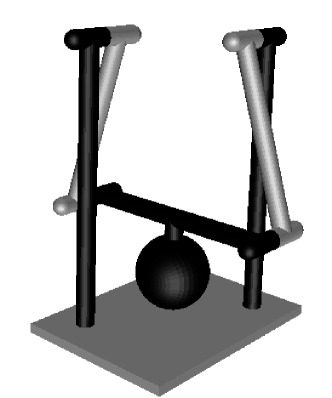
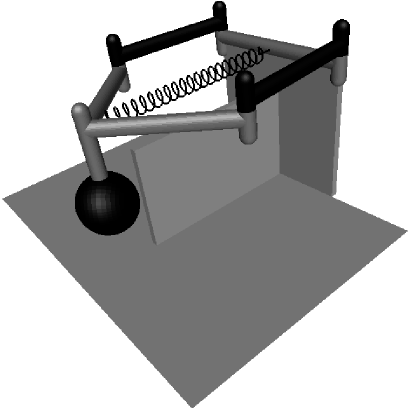
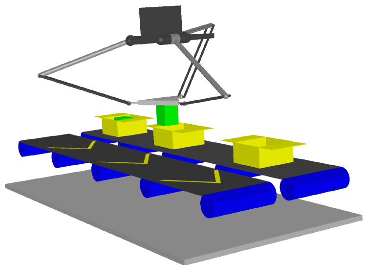
Figure 5: Test cases used to validate the planner: a four-bar pendulum (top-left), a five-bar robot (top-right), and a Delta robot (bottom).

VI Test Cases

The planner has been implemented in C and integrated in the CUIK Suite [45]. We next illustrate its performance in three test cases of increasing complexity (Fig. 5). The first case was already mentioned in the introduction. It consists of a planar four-bar pendulum with limited motor torque that has to move a load. The robot may need to oscillate several times to move between the two states shown in Fig. 1. The second test case involves a planar five-bar robot equivalent to the Dextar prototype [10], but with an added spring to enhance its compliance. The goal here is to move the load from one side to the other of a wall, with null initial and final velocities. Unlike in the first case, collisions may occur here, and thus they should be avoided. In the third case, a Delta robot moves a heavy load in a pick-and-place scenario. It picks up the load from a conveyor belt moving at constant velocity, and places it at rest inside a box on a second belt. In contrast to typical Delta robot applications, here the weight of the load is considerable, which increases dynamics effects substantially. Table I summarizes the problem dimensions, parameters, and performance statistics of all test cases. The full set of geometric and dynamic parameters will be made available online in the final version of the paper.

TABLE I: Test case dimensions, parameters, and performance statistics.

Robot	$n_{q}$	$n_{e}$	$d_{\mathcal{C}}$	$d_{\mathcal{X}}$	No. of actions	$\tau_{max}$ [Nm]	$\beta$	No. of samples	No. of charts	Exec. Time [s]
Four-Bars	4	3	1	2	3	16	0.1	452	122	2.7
	4	3	1	2	3	12	0.1	569	145	3.4
	4	3	1	2	3	8	0.1	1063	195	6.3
	4	3	1	2	3	4	0.1	2383	248	14.2
Five-Bars	5	3	2	4	5	0.1	0.25	15980	101	124
Delta	15	12	3	6	7	1	0.5	1654	58	183

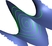
Figure 6: From left to right, the state manifold (in blue), and the trajectory obtained (green) for a maximum torque $\tau_{max}$ of 16, 12, 8, and 4 [Nm].

In this paper, relative joint angles are used to formulate Eq. (1). As the three robots involve $n_{q}=4$, $5$, and $15$ joints, and each independent kinematic loop introduces $3$ or $6$ constraints (depending on whether the robot is planar or spatial), the dimensions of the C-space are $d_{\mathcal{C}}=1$, $2$, and $3$, respectively. For the formulation of the dynamic equations, the Euler-Lagrange equations with multipliers are used. Friction forces can be easily introduced in this formulation, but we have neglected them.

The robots respectively have $n_{u}=1$, $2$, and $3$ of their base joints actuated, while the remaining joints are passive. Following LaValle and Kuffner [36], the set $\mathcal{U}$ is discretized in a way reminiscent of bang-bang control schemes. Specifically, $\mathcal{U}$ will contain all possible actions $u$ in which only one actuator is active at a time, with a torque that can be -$\tau_{max}$ or $\tau_{max}$. Additionally, $\mathcal{U}$ also includes the action where no control is applied and the system simply drifts. As shown in Table I, this results in sets $\mathcal{U}$ of $3$, $5$, and $7$ actions, respectively. The table also gives the $\tau_{max}$ values for each case.

In all test cases the parameters are set to $t_{m}=0.1$, $\delta=0.05$, $\rho_{s}=d_{\mathcal{C}}$, $\rho=\rho_{s}/2$, $\cos(\alpha)=0.1$, and $\epsilon=0.1$. The value $\beta$ is problem-specific and given in Table I. The table also shows the performance statistics on an iMac with a Intel i7 processor at 2.93 Ghz with 8 CPU cores, which are exploited to run lines 2 to 2 of Algorithm 2 in parallel. The statistics include the number of samples and charts, as well as the execution times in seconds, all averaged over ten runs. The planner successfully connected the start and goal states in all runs.

In the case of the four-bar mechanism, results are included for decreasing values of $\tau_{max}$. As reflected in Table I, the lower the torque, the harder the planning problem. The solution trajectory on the state-space manifold (projected in one position and two velocity variables) can be seen in Fig. 6 for the different values. Clearly, the number of oscillations needed to reach the goal is successively higher. The trajectory obtained for the most restricted case is shown in Fig. 7, top.

In the five-bars robot, although it only has one more link than the previous robot, the planning problem is significantly more complex. This is due to the narrow corridor created by the obstacle to overcome. Moreover, the motors have a severely limited torque taking into account the spring constant. In order to move the weight in such conditions, the planner is forced to increase the momentum of the payload before overpassing the obstacle, and to decrease it once it is passed so as to reach the goal configuration with zero velocity (Fig. 7, middle). This increased complexity is reflected in the number of samples and the execution time needed to solve the problem. However, the number of charts is low, which shows that the planner is not exploring new regions of the state space, but trying to find a way through the narrow corridor.

Finally, the table gives the same statistics for the problem on the Delta robot. The execution time is higher due to the increased complexity of the problem. The robot is spatial, it has a state space of dimension $6$ in an ambient space of dimension $30$, and involves more kinematic constraints than in the previous cases. Moreover, given the velocity of the belt, the planner is forced to reduce the initial momentum of the load before it can place it inside the box (Fig. 7, bottom).

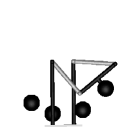
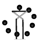
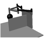
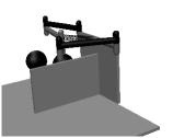
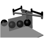
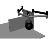
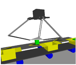
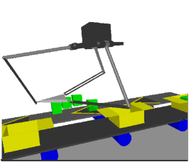
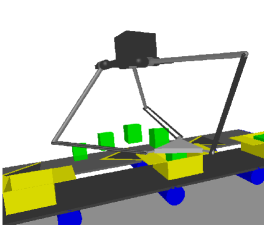
Figure 7: Snapshots of the trajectories obtained by the planner for the three test cases. Video animations can be seen in the multimedia files of this paper.

VII Conclusions

This paper has proposed an RRT planner for dynamical systems with implicitly defined state spaces. Dealing with such spaces presents two major hurdles: the generation of random samples in the state space and the driftless simulation over such space. We have seen that both issues can be properly addressed by relying on local parameterizations. The result is a planner that navigates the state space manifold following the vector fields defined by the dynamic constraints on such manifold. The presented experiments show that the proposed method can successfully solve significantly complex problems. In the current implementation, however, most of the time is used in computing dynamics-related quantities. The use of specialized dynamical simulation libraries may alleviate this issue [53, 21].

To scale to even more complex problems, several aspects of the proposed RRT planner need to be improved. Probably the main issue is the metric used to measure the distance between states. This is a general issue of all sampling-based kinodynamic planners, but in our context it is harder since the metric should not only consider the vector fields defined by the dynamic constraints, but also the curvature of the state space manifold defined by the kinematic equations. Using a metric derived from geometric insights provided by the kinodynamic constraints may result in significant performance improvements. In a broader context, another aspect deserving attention is the analysis of the proposed algorithm, in particular its completeness and the optimality of the resulting trajectory. The former should derive from the properties of the underlying planners. With respect to the latter, locally optimal trajectories could be obtained using the output of the planner to feed optimization approaches [46, 12], or globally optimal ones considering the trajectory cost into the planner [24, 38]. Finally, the relation of the proposed approach with variational integration methods [40, 28] should also be examined.

References

- Barraquand and Latombe [1991] J. Barraquand and J. C. Latombe. Nonholonomic multibody mobile robots: controllability and motion planning in the presence of obstacles. In IEEE International Conference on Robotics and Automation, volume 3, pages 2328–2335, 1991.
- Bauchau and Laulusa [2008] O. A. Bauchau and A. Laulusa. Review of contemporary approaches for constraint enforcement in multibody systems. Journal of Computational and Nonlinear Dynamics, 3(1):011005, 2008.
- Baumgarte [1972] J. Baumgarte. Stabilization of constraints and integrals of motion in dynamical systems. Computer Methods in Applied Mechanics and Engineering, 1(1):1–16, 1972.
- Berenson et al. [2011] D. Berenson, S. Srinivasa, and J. J. Kuffner. Task space regions: A framework for pose-constrained manipulation planning. International Journal of Robotics Research, 30(12):1435–1460, 2011.
- Betts [2010] J. T. Betts. Practical Methods for Optimal Control and Estimation Using Nonlinear Programming. SIAM Publications, 2010.
- Blajer [2002] W. Blajer. Elimination of constraint violation and accuracy aspects in numerical simulation of multibody systems. Multibody System Dynamics, 7(3):265–284, 2002.
- Bohigas et al. [2013] O. Bohigas, M. E. Henderson, L. Ros, M. Manubens, and J. M. Porta. Planning singularity-free paths on closed-chain manipulators. IEEE Transactions on Robotics, 29(4):888–898, 2013.
- Bohigas et al. [2016] O. Bohigas, M. Manubens, and L. Ros. Singularities of robot mechanisms: numerical computation and avoidance path planning, volume 41 of Mechanisms and Machine Science. Springer, 2016.
- Bohlin and Kavraki [2000] R. Bohlin and L. E. Kavraki. Path planning using lazy PRM. In IEEE International Conference on Robotics and Automation, volume 1, pages 521–528, 2000.
- Bourbonnais et al. [2015] F. Bourbonnais, P. Bigras, and I. A. Bonev. Minimum-time trajectory planning and control of a pick-and-place five-bar parallel robot. IEEE/ASME Transactions on Mechatronics, 20(2):740–749, 2015.
- Braun and Goldfarb [2009] D. J. Braun and M. Goldfarb. Eliminating constraint drift in the numerical simulation of constrained dynamical systems. Computer Methods in Applied Mechanics and Engineering, 198(37–40):3151–3160, 2009.
- Butler et al. [2016] S. D. Butler, M. Moll, and L. E. Kavraki. A general algorithm for time-optimal trajectory generation subject to minimum and maximum constraints. In Workshop on the Algorithmic Foundations of Robotics, 2016.
- Canny [1988] J. Canny. Some algebraic and geometric computations in PSPACE. In ACM Symposium on Theory of Computing, pages 460–467, 1988.
- Cheng [2005] P. Cheng. Sampling-based motion planning with differential constraints. Phd dissertation, Department of Computer Science, University of Illinois, 2005.
- Cheng and LaValle [2001] P. Cheng and S. M. LaValle. Reducing metric sensitivity in randomized trajectory design. In IEEE/RSJ International Conference on Intelligent Robots and Systems, volume 1, pages 43–48, 2001.
- Cheng and LaValle [2002] P. Cheng and S. M. LaValle. Resolution complete rapidly-exploring random trees. In IEEE International Conference on Robotics and Automation, volume 1, pages 267–272, 2002.
- Cherif [1999] M. Cherif. Kinodynamic motion planning for all-terrain wheeled vehicles. In IEEE International Conference on Robotics and Automation, volume 1, pages 317–322, 1999.
- Choset et al. [2005] H. Choset, K. M. Lynch, S. Hutchinson, G. A. Kantor, W. Burgard, L. E. Kavraki, and S. Thrun. Principles of Robot Motion: Theory, Algorithms, and Implementations. Intelligent Robotics and Autonomous Agents. MIT Press, 2005.
- Donald et al. [1993] B. Donald, P. Xavier, J. Canny, and J. Reif. Kinodynamic motion planning. Journal of the ACM, 40(5):1048––1066, 1993.
- Dubowsky and Shiller [1985] S. Dubowsky and Z. Shiller. Optimal dynamic trajectories for robotic manipulators. In IFToMM Symposium on Robot Design, Dynamics and Control, pages 133–143, 1985.
- Georgia Tech and Carnegie Mellon University [2017] Georgia Tech and Carnegie Mellon University. DART: Dynamic animation and robotics toolkit. https://dartsim.github.io, 2017.
- Hairer [2001] E. Hairer. Geometric integration of ordinary differential equations on manifolds. BIT Numerical Mathematics, 41(5):996–1007, 2001.
- Hairer et al. [2006] E. Hairer, C. Lubich, and G. Wanner. Geometric numerical integration: structure-preserving algorithms for ordinary differential equations, 2006.
- Hauser and Zhou [2016] K. Hauser and Y. Zhou. Asymptotically optimal planning by feasible kinodynamic planning in a state-cost space. IEEE Transactions on Robotics, 32(6):1431–1443, 2016.
- Henderson [2002] M. E. Henderson. Multiple parameter continuation: computing implicitly defined k-manifolds. International Journal of Bifurcation and Chaos, 12(3):451–476, 2002.
- Jaillet and Porta [2013] L. Jaillet and J. M. Porta. Path planning under kinematic constraints by rapidly exploring manifolds. IEEE Transactions on Robotics, 29(1):105–117, 2013.
- Jaillet et al. [2011] L. Jaillet, J. Hoffman, J. van den Berg, P. Abbeel, J. M. Porta, and K. Goldberg. EG-RRT: Environment-guided random trees for kinodynamic motion planning with uncertainty and obstacles. In IEEE/RSJ International Conference on Intelligent Robots and Systems, pages 2646–2652, 2011.
- Johnson and Murphey [2009] E. R. Johnson and T. D. Murphey. Scalable variational integrators for constrained mechanical systems in generalized coordinates. IEEE Transactions on Robotics, 25(6):1249–1261, 2009.
- Kalakrishnan et al. [2011] M. Kalakrishnan, S. Chitta, E. Theodorou, P. Pastor, and S. Schaal. STOMP: Stochastic trajectory optimization for motion planning. In 2011 IEEE International Conference on Robotics and Automation, pages 4569–4574, 2011.
- Kalisiak [2008] M. Kalisiak. Toward more efficient motion planning with differential constraints. PhD thesis, Computer Science,University of Toronto, 2008.
- Kavraki et al. [1996] L. E. Kavraki, P. Svestka, J.-C. Latombe, and M. H. Overmars. Probabilistic roadmaps for path planning in high-dimensional configuration spaces. IEEE Transactions on Robotics and Automation, 12(4):566–580, 1996.
- Ladd and Kavraki [2005] A. M. Ladd and L. E. Kavraki. Fast tree-based exploration of state space for robots with dynamics. In Algorithmic Foundations of Robotics VI, pages 297–312, 2005.
- Latombe [1991] J.-C. Latombe. Robot Motion Planning. Engineering and Computer Science. Springer, 1991.
- Laulusa and Bauchau [2008] A. Laulusa and O. A. Bauchau. Review of classical approaches for constraint enforcement in multibody systems. Journal of Computational and Nonlinear Dynamics, 3(1):011004, 2008.
- LaValle [2006] S. M. LaValle. Planning Algorithms. Cambridge University Press, New York, 2006.
- LaValle and Kuffner [2001] S. M. LaValle and J. J. Kuffner. Randomized kinodynamic planning. International Journal of Robotics Research, 20(5):378–400, 2001.
- Lee [2001] J. M. Lee. Introduction to Smooth Manifolds. Springer, 2001.
- Li et al. [2016] Y. Li, Z. Littlefield, and K. E. Bekris. Asymptotically optimal sampling-based kinodynamic planning. The International Journal of Robotics Research, 35(5):528–564, 2016.
- Lynch and Mason [1996] K. M. Lynch and M. T. Mason. Stable pushing: mechanics, controllability, and planning. The International Journal of Robotics Research, 15(6):533–556, 1996.
- Marsden and West [2001] J. E. Marsden and M. West. Discrete mechanics and variational integrators. Acta Numerica 2001, 10:357–514, 2001.
- Petzold [1992] L. R. Petzold. Numerical solution of differential-algebraic equations in mechanical systems simulation. Physica D: Nonlinear Phenomena, 60(1–4):269–279, 1992.
- Pham et al. [2017] Q.-C. Pham, S. Caron, P. Lertkultanon, and Y. Nakamura. Admissible velocity propagation: Beyond quasi-static path planning for high-dimensional robots. The International Journal of Robotics Research, 36(1):44–67, 2017.
- Plaku et al. [2007] E. Plaku, L. Kavraki, and M. Vardi. Discrete search leading continuous exploration for kinodynamic motion planning. In Proceedings of Robotics: Science and Systems, 2007.
- Porta et al. [2012] J. M. Porta, L. Jaillet, and O. Bohigas. Randomized path planning on manifolds based on higher-dimensional continuation. The International Journal of Robotics Research, 31(2):201–215, 2012.
- Porta et al. [2014] J. M. Porta, L. Ros, O. Bohigas, M. Manubens, C. Rosales, and L. Jaillet. The Cuik Suite: Analyzing the motion closed-chain multibody systems. IEEE Robotics and Automation Magazine, 21(3):105–114, 2014.
- Posa et al. [2016] M. Posa, S. Kuindersma, and R. Tedrake. Optimization and stabilization of trajectories for constrained dynamical systems. In IEEE International Conference on Robotics and Automation, pages 1366–1373, 2016.
- Potra and Yen [1991] F. A. Potra and J. Yen. Implicit numerical integration for Euler-Lagrange equations via tangent space parametrization. Journal of Structural Mechanics, 19(1):77–98, 1991.
- Reif [1979] J. H. Reif. Complexity of the mover’s problem and generalizations. In Annual Symposium on Foundations of Computer Science, pages 421–427, 1979.
- Schulman et al. [2014] J. Schulman, Duan Y, J. Ho, A. Lee, I. Awwal, H. Bradlow, J. Pan, S. Patil, K. Goldberg, and P. Abbeel. Motion planning with sequential convex optimization and convex collision checking. The International Journal of Robotics Research, 33(9):1251–1270, 2014.
- Shkolnik et al. [2009] A. Shkolnik, M. Walter, and R. Tedrake. Reachability-guided sampling for planning under differential constraints. In IEEE International Conference on Robotics and Automation, pages 2859–2865, 2009.
- Stilman [2007] M. Stilman. Task constrained motion planning in robot joint space. In IEEE/RSJ International Conference on Intelligent Robots and Systems, pages 3074–3081, 2007.
- Şucan and Kavraki [2012] I. A. Şucan and L. E. Kavraki. A sampling-based tree planner for systems with complex dynamics. IEEE Transactions on Robotics, 28(1):116–131, 2012.
- The Neuroscience and Robotics Lab, Northwestern University [2016] The Neuroscience and Robotics Lab, Northwestern University. Trep: Mechanical simulation and optimal control. http://murpheylab.github.io/trep, 2016.
- Zucker et al. [2013] M. Zucker, N. Ratliff, A. D. Dragan, M. Pivtoraiko, M. Klingensmith, C. M. Dellin, J. A. Bagnell, and S. S. Srinivasa. CHOMP: Covariant Hamiltonian optimization for motion planning. The International Journal of Robotics Research, 32(9-10):1164–1193, 2013.