The grasshopper problem
Abstract
We introduce and physically motivate the following problem in geometric combinatorics, originally inspired by analysing Bell inequalities. A grasshopper lands at a random point on a planar lawn of area one. It then jumps once, a fixed distance , in a random direction. What shape should the lawn be to maximise the chance that the grasshopper remains on the lawn after jumping? We show that, perhaps surprisingly, a disc shaped lawn is not optimal for any . We investigate further by introducing a spin model whose ground state corresponds to the solution of a discrete version of the grasshopper problem. Simulated annealing and parallel tempering searches are consistent with the hypothesis that for the optimal lawn resembles a cogwheel with cogs, where the integer is close to . We find transitions to other shapes for .
I Introduction
I.1 Relation to Bell inequalities
As Bell’s celebrated theorem Bell (1964) showed, quantum theory is not locally causal. The correlations predicted by quantum theory for the results of spacelike separated measurements on two or more entangled systems cannot be reproduced by any locally causal model. Bell inequalities are constraints on correlations, for some set of measurements, that must be satisfied by any locally causal model but are violated when those measurements are carried out on some quantum states. Simple Bell inequalities, such as the Clauser-Horne-Shimony-Holt inequality Clauser et al. (1969), demonstrate the gap between the predictions of quantum theory and locally causal theories in a form that can be experimentally verified, even after allowing for detector inefficiencies and errors.
However, the full class of Bell inequalities remains poorly understood, even for the simplest case of spin measurements on two spin particles. Understanding more general Bell inequalities is intrinsically interesting, shedding light as it does on the structure and properties of quantum theory. There is also some practical motivation, since many quantum cryptographic protocols and tests depend on Bell inequalities to verify that a shared quantum state yields quantum correlations of the right type. This is necessary in many scenarios since such a state may have been supplied by an untrustworthy party or interfered with by an eavesdropper. Optimizing protocols requires considering the full class of Bell inequalities. One might expect that inequalities that involve completely random measurement choices are good options, since they give adversaries minimal information.
With these motivations, Ref. Kent and Pitalúa-García (2014) introduced and analysed Bell inequalities for the case where two parties carry out spin measurements about randomly chosen axes and obtain the spin correlations for pairs of axes separated by angle , for each in the range . It was shown that the correlations of locally causal models satisfy bounds violated by quantum theory for in the range . Although the bounds obtained were shown to be optimal for an infinite set of values of converging to zero, they were not shown to be optimal for general , and indeed we expect that they are not. It was noted Kent and Pitalúa-García (2014) that obtaining tight bounds would be equivalent to solving a geometric combinatorics problem on the Bloch sphere. In its simplest form (which assumes an additional ansatz about the solution) this problem can be pictured as follows. Half the area of a sphere is covered by a lawn, with the property that exactly one of every pair of antipodal points belongs to the lawn. A grasshopper lands at a random point on the lawn, and then jumps in a random direction through spherical angle . What lawn shape maximises the probability that the grasshopper remains on the lawn after jumping, and what is this maximum probability (as a function of )?
The problem seems harder to solve than to pose. Intuitions and sketchy ideas for proofs come readily to mind, but these may well be incorrect.111The lion and man problem, which asks whether a lion can always catch a man in a bounded region if they have equal maximum speeds and the man wishes to avoid capture, gives a well known cautionary example of the pitfalls of intuitive reasoning: see pp. 114-117 of Ref. Littlewood and Bollobás (1986). One common initial intuition is that the problem has an isoperimetric flavour. It appears at first glance that minimizing the length of the lawn boundary might also minimize the probability of jumping outside the lawn, at least for small . If so, a hemispherical lawn would be optimal for small . However, this proof idea neglects the possibility that a jump could cross the boundary twice or more.
I.2 The planar grasshopper problem
Another intuition is that the problem may be simpler to solve if translated to the plane. This means dropping the antipodal condition, which has no simple analogue for the planar version of the problem. Investigating the planar problem thus also tests the relevance of the antipodal condition. A related intuition is that the disc should be provably optimal for small jumps in the plane, whether or not there is an isoperimetric argument for this.
However, as far as we have been able to establish, not only is the answer to the planar grasshopper problem not known, but the question does not seem to have ever been studied. This seems surprising, given that the question could have been posed by Euclid and might plausibly have interested him and contemporaries.222There is perhaps some question as to how precisely Euclid understood the notion of randomness, although he certainly used the term; vide Proposition II.4 of Ref. Euclid . An interesting discussion can be found at https://rjlipton.wordpress.com/2016/01/12/did-euclid-really-mean-random/ . Remarkably, no even vaguely similar question appears in Croft et al.’s survey Croft et al. (1991) of unsolved problems in geometry. The closest results of which we are aware are those of Bukh Bukh (2008), which describe the properties of sets in that have no pair of points separated by any of some finite list of distances.
From the perspective of geometric combinatorics, the planar version of the grasshopper problem seems the most natural starting point. It is intriguing in its own right, and as we will see, has an unexpectedly rich structure. It also tests out intuitions that could be formed about the spherical problem, without the extra conditions relevant to Bell inequalities. For example, if a pure isoperimetric argument could somehow be run in the spherical case, without appealing to the extra conditions, intuition suggests a similar argument should work in the planar case. In particular, if it were possible to show by a purely isoperimetric argument that a hemisphere is optimal on a sphere (of area ) for small jump angles , then one would also expect the disc to be optimal in the plane for small jump distances . However, as we will see, the disc is not optimal in the plane for any . So, any proof idea for the spherical problem needs either to identify non-hemispherical optimal solutions and explain why they are optimal, or to go beyond isoperimetric intuitions, or to explain why the spherical case is different, or to explain why the extra conditions matter.
The planar problem is also the simplest and most natural setting for exploring experimental approaches to the problem based on discretizing it and reformulating the discretization in terms of statistical physical spin models, which we describe below. These spin models are interesting in their own right, as they represent an unusual class of systems with fixed-range interactions, where the range can be large. Discretizing the problem also raises theoretical and computational issues, which are best explored in the simplest setting. In this paper, we thus focus on the planar problem. We explain the numerical techniques used, and the various consistency checks that allow reasonable confidence that our results are at least qualitatively broadly correct. We then describe and analyse these results. We leave the application of the techniques developed here to the spherical and other cases for future work.
II Statement of the main problem
Informal statement: You are given a bag of grass seed from which you can grow a lawn of any shape (not necessarily connected) with unit area on a planar surface. A grasshopper lands at a random point on your lawn, then jumps a given distance in a random direction. What lawn shape should you choose to maximise the probability that the grasshopper remains on your lawn after jumping?
The lawn may also be allowed to be of variable density, between zero and one, with the condition that the integrated density over the plane is one. In this case, we take the probability density for the grasshopper to land at a specific point on the lawn to be the lawn density at this point. Likewise we take the probability that the grasshopper remains on the lawn after jumping to be the lawn density at its landing point.
Formal statement: Consider a probability density on the plane satisfying for all and
| (1) |
The functional is defined by
with the unit vector . What is the supremum of over all such density functions , for each value of ? Which , if any, attain the supremum? Or if none, which sequences approach the supremum value?
For most of this paper we focus on the case where the lawn density takes only the values or , i.e. the lawn is a shape of area and uniform density. This is a natural version of the problem. Moreover, as we explain below, investigating it also gives a great deal of insight into the general case.
Formulation in Fourier space: It is illuminating to recast the functional defined in Eq. (II) in terms of the Fourier transform of the density function , defined via and . The normalisation condition (1) then implies . In this representation the functional is
| (3) |
where is the Bessel function of the first kind. Note that if is an even function, then is real and even and if is radially symmetric then is real and radially symmetric also.
Success probability for the unit disc lawn: The success probability for lawns in the shape of the unit disc (with density one inside the disc and zero outside) can be calculated exactly by analytically solving the integral (II) for , or equivalently the integral (3) for ,
| (4) |
assuming . Its Taylor expansion for small is
| (5) |
The success probability approaches one as and decreases monotonically with increasing .
III Analytic results
Lemma 1: The disc of area (radius ) is not optimal for any .
Proof: Suppose and suppose that the lawn is the disc of area centred at the origin. If the grasshopper lands within the disc of radius centred at the origin, then its jump will take it outside with probability . Removing from and redistributing its area to some shape outside thus cannot lower the overall success probability. Moreover, it is easy to find shapes that increase the overall success probability. For (a far from optimal) example, one could take to be a rectangle, lying anywhere outside , of width and height , where is chosen so that .
Comment: This argument clearly fails for , suggesting that we might expect different types of solution in the regimes and . The construction also suggests that solutions for might fail to be simply connected, since it begins by creating a hole in the centre of the disc. In fact, we show below that the disc is not optimal even for , so that the construction does not directly apply and does not necessarily imply a transition at precisely . However, our results also suggest that for above and close to the optimal solution is not simply connected, or even connected.
Lemma 2: There exists an infinite sequence of jumps , with for all positive integer and , such that for each the disc of area is not optimal.
Comment: The intuition that the disc should be optimal for sufficiently small is thus incorrect.
Proof: Let for . This gives for , so Lemma already shows the disc is not optimal for these cases. Note that for , is the edge length of a polygon with edges inscribed in the unit disc. For , choose parameters such that and , so that the perimeter of the unit disc is . Take to be small.
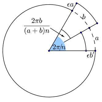
A shape of area can be constructed as follows, see Fig. 1. In polar coordinates , is defined by the disc segments
| (6) | |||||
for integer in the range . Here is determined by the area condition, which gives us
| (7) |
Fix and then fix satisfying the conditions above. Now, since is small, we can consider as a close approximation to , and calculate the difference in their success probabilities to lowest non-zero order in ; it turns out we do not need the higher order terms in .
Calculating the difference in the relevant integrals gives that the difference in success probabilities is
| (8) |
For and sufficiently small this is positive. Hence the disc is also not optimal for when .
Comment: We see that perturbing the disc by alternating thin protrusions and thicker indentations, producing a shape with -fold rotational symmetry, gives a higher success probability when
| (9) |
and so for large . In fact, our numerical results from statistical modelling are consistent with the hypothesis that the optimal shape has -fold symmetry, approximately related to as above, for all . We describe these results in Sec. VI.1.
Theorem 3: The disc of area is not optimal for any .
Proof: For this is already established by Lemma and for it is established by Lemma . To prove that the disc is not optimal for in the range we consider for positive integers with no common divisor such that and . In this construction, is the edge length of an regular stellated polygon, where is the number of vertices and is the winding number around the centre. Hence there are vertices between each two vertices separated by the edge of length .
As before, choose parameters such that and , so that the perimeter of the unit disc is , and take to be small. A shape of area can be constructed as in the proof of Lemma 2. Fix and then fix satisfying the conditions above. As in the proof of Lemma 2, we take small, so that is a close approximation to . The difference in their success probabilities to lowest non-zero order in is also given by expression (8), as before.
For and sufficiently small the probability difference (8) is positive and hence the disc is not optimal for . By continuity, there is a neighbourhood of each for which the disc is also not optimal. But the form a dense subset of the interval . Hence the disc is not optimal for any .
Comment: Lawn shapes with protrusions and indentations can be constructed as described above, where approximately solve
| (10) |
We can thus approximate a given value of either by (9) or (generally more closely) by (10) with . Our argument implies that, for that value of and some approximation (10), there is a shape with the symmetries of the stellated polygon that has higher probability than the disc. However, it does not imply that any such shape is necessarily optimal. Numerically the best shapes found have a -fold degree of symmetry, where the integer is close to the solution of (9) and hence smaller than the obtained from the stellated construction (10). This was seen numerically even in the cases where the solution of (9) was close to a half-integer. In such cases both the next-highest and the next-lowest integer approximations give a higher success probability than the solution from (10). We describe these results in Sec. VI.1; see in particular Fig. 5.
Comment: Suppose that the optimal solution for jump is given by a density one lawn whose shape has a smooth boundary. Consider two points on the boundary of and the circles of radius centred at . Let , and let be the sum of the lengths of the arcs comprising , for .
We now give an unrigorous argument that . Suppose this is not the case, and without loss of generality that . Then, by continuity, analogous inequalities hold for points (inside or outside ) in small neighbourhoods of and . Subtracting a small area from that includes and adding the same area to the exterior of the boundary of around then should increase the success probability, which would contradict the optimality of .
This observation suggests what we will call the equal arc length hypothesis Lentner : for any given , the sum of the arc lengths for is identical for all points on the boundary of the optimal shape . Of course, the disc satisfies the equal arc length hypothesis for all . The best shapes found numerically also appear approximately consistent with the hypothesis, although the current numerical resolution is not high enough to give compelling evidence. We leave further investigation for future work.
IV Spin model for the discrete grasshopper problem
We define a discrete version of the grasshopper problem by dividing the plane into grid cells and assigning a spin variable to the centre of each cell , where and correspond to the cell being unoccupied or occupied by the lawn, respectively. Here we only consider regular lattices, for which all cells have the same area . The area one condition for the lawn then corresponds to a fixed number of spins having value , so that we have .
If we treat a discretized lawn as simply a restricted case of the general problem, its success probability is defined by Eq. (II). However, we aim to identify approximate solutions to the grasshopper problem by using simple statistical physics models that involve quantities that can be computed more quickly. To do this, we discretize the functional in Eq. (II), such that in the continuum limit ( and , keeping the total area fixed) the discrete functional approaches the exact continuous expression. We have the following correspondence between continuous and lattice quantities:
| (11) | |||||
| (12) | |||||
| (13) |
Here are the positions of the sites of the lattice and is the lattice spacing, which scales like (for a square lattice ). The discretization involves a smoothed approximation to the (one-dimensional) -function, which appears in (II). We can construct through a continuous function with finite support and unit integral in the following manner,
| (14) |
With this definition as . The function must fulfill certain additional conditions, which are introduced and motivated in Ref. Peskin (2002), to compensate as much as possible for the inaccuracy associated with the presence of the discrete grid. Here we use two alternative definitions of , given by Eqs. (16, 17), extensive tests of which can be found in Ref. Yang et al. (2009).
The discrete version of the functional then becomes
| (15) |
In the continuum limit, . To resolve the jump distance we require . We look for spin configurations that maximise , which represent solutions to the discrete grasshopper problem considered.
This problem is equivalent to finding the ground state of a spin system with Hamiltonian . The range of the interactions for this Hamiltonian is fixed, but not nearest neighbour. It is thus an Ising model with fixed total spin Newman and Barkema (1999) and with fixed-range attractive interactions. The interaction range is approximately the grasshopper jump distance , modulo small variations introduced by the discretization of the delta function. To the best of our knowledge, systems with interactions that have a fixed range significantly larger than the lattice spacing have not been studied before. Our results suggest this class of statistical models have some interesting and unusual properties.
V Numerical Setup
Our discretization involves theoretical choices: the type of lattice, the number of occupied sites, and the precise form of the -function approximation . The default setup is a square grid with fixed total spin and grid cell size (lattice spacing) determined by the area one condition: . We varied the lattice spacing by performing simulations for several different between 5000 and 90000, corresponding to between approximately 0.015 and 0.003. As the default, we use the following approximation to the -function Peskin (2002),
| (16) |
This means that two occupied lattice sites contribute to if the absolute difference between their distance and is at most lattice spacings. The contribution is larger the closer the distance is to . To assess the effect of the -function discretization we also performed calculations with a different choice for , discussed in Yang et al. (2009),
| (17) |
To check whether the structure of the lattice affects the optimal lawn shape, we also simulated the model on a hexagonal grid. In this case the area of a grid cell is , where the lattice spacing is the distance between the centres of the hexagonal cells.
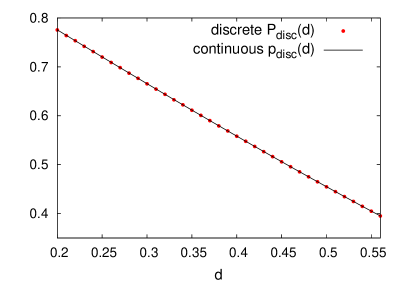
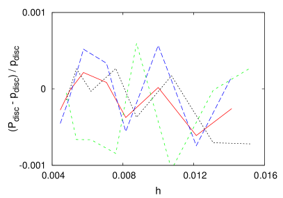
To illustrate the effects of discretization and the specific setup, Fig. 2 shows the dependence of for the unit disc on the discretization parameters, in comparison to the exact continuous model probability (4). For all setups considered the results agree well with each other and the deviation from the continuous solution is of order or less. Discretization effects for the best configurations found numerically are discussed in Sec. VI.1.
We use simulated annealing Kirkpatrick et al. (1983) and parallel tempering Hukushima and Nemoto (1996) to find configurations that maximise for different values of . For this we introduce an additional simulation parameter , which is the analogue of a temperature. At fixed temperature, in each simulation step the spin configuration is updated as follows Newman and Barkema (1999). We select a random lattice site with and a random lattice site with . We then attempt to exchange the spin values such that and . The exchange is accepted with the Metropolis acceptance probability and rejected with probability . Here is the difference between the values of the new and the old configuration. If the update is deterministically accepted, otherwise it can still be accepted with a probability that exponentially decreases as a function of . The higher the temperature, the likelier are we to accept an update that decreases . At low temperatures, when the acceptance rate is low, it can be advantageous to use continuous time Monte Carlo updates instead. In this case the pair of lattice sites is selected according to their pre-calculated exchange probability, rather than uniformly, and the exchange is then deterministically accepted Newman and Barkema (1999). Since here we are only interested in the final zero temperature state, we do not need to keep track of the Monte Carlo time.
For a simple simulated annealing search, we start the simulation with a random spin configuration at high temperature and then gradually decrease the temperature until a minimal temperature is reached. We use an exponential cooling schedule: at each annealing round the temperature is multiplied by a constant factor . The number of simulation steps between the annealing rounds must be large enough to allow the system to reach a stationary state. Several animations showing examples of the annealing process can be found in the Supplemental Material. While simulated annealing is effective at identifying global extrema for many systems, it can fail, particularly for rugged energy landscapes.
In parallel tempering, also known as replica exchange Monte Carlo, several copies of the system are simulated in parallel, each at a different fixed temperature. After some number of steps, exchange updates attempting to swap configurations at neighboring temperatures are suggested. The acceptance probability for the swap updates is min, where is the inverse temperature. This method is generally more successful in probing complex energy landscapes, since through exchanging configurations with those at higher temperatures the system can escape from local extrema. Nevertheless, no statistical method is guaranteed to find a global extremum.
We performed extensive tests to find optimal annealing and parallel tempering schedules and performed several independent simulations for each set of parameters. To establish the best shape for values of for which our results were ambiguous, for instance near a transition between two different types of shape with similar values of , we performed additional checks: each potentially optimal solution was set as the initial configuration, and the annealing process was then run with a sufficiently low starting temperature to ensure that the rough shape was preserved, while attempting to further optimize .
VI Numerical results
All results presented in this section were obtained with a square grid, and the -function approximation given by Eq. (16), unless stated otherwise. Checks were also performed with alternative setups (hexagonal grid, , different values of up to ) and produced consistent results.
VI.1 Cogwheel regime


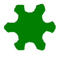
We first consider . Figure 3 shows the best configurations found for between and . These configurations have dihedral symmetry with a shape resembling a cogwheel. In particular, the cogwheel was always found superior to the disc shape and was produced even if the starting configuration was initialized in the shape of a unit disc (at sufficiently low temperature) rather than a random distribution at high temperature. This is consistent with our analytical results presented in Sec. III.


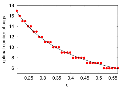
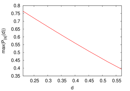
The optimal number of cogs, , was found to decrease with increasing and is well-described by the relation (9). However, the number of cogs is discrete while can take any real value. The optimal closely corresponds to the nearest integer satisfying (9). If the solution of (9) is close to a half-integer, the optimal number of cogs is difficult to identify precisely from the simulations: the best cogwheels found with either of the two closest integer solutions to (9) yield very similar values of . An example of two configurations with nearly the same but with different numbers of cogs is shown in Fig. 4 for . The exact solution of (9) is in this case, and hence and are almost equally good approximations. Figure 5 shows the optimal number of cogs in the simulations as a function of , and the highest found.
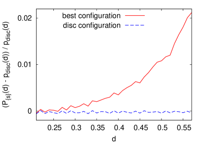
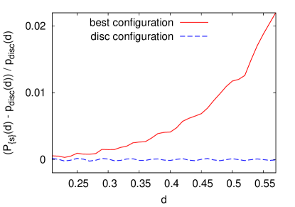
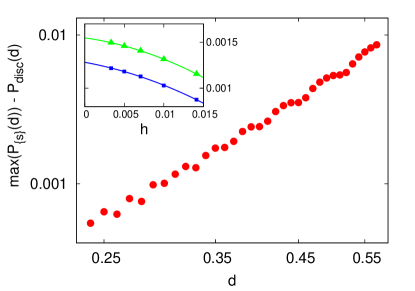
The results remained consistent for all setups and parameter values studied. Moreover, the orientation of the cogwheel configurations with respect to the grid was different for independent simulation runs and appeared uncorrelated with the symmetry axes of the grid. This was the case also for the configurations at higher discussed in the following sections. At low , the difference in the values of for the best cogwheel configurations found and the disc shaped configurations was very small. In particular, it was sometimes found to be smaller than the fluctuations due to the discretization that are shown in Fig. 2. These fluctuations, however, appear to be strongly correlated for the two types of configuration, and the cogwheel was found to be consistently superior to the disc for all and in all discretization setups considered, see Fig. 6. At larger fluctuations become milder and the difference between the cogwheel and the disc configurations becomes more pronounced. Figure 7 shows the difference between the values of for the best cogwheel and the disc configurations, plotted as a function of on a double-logarithmic scale. This difference was calculated independently for several lattice spacings and then extrapolated to the continuum limit . It is always positive and appears to be roughly a straight line on large scale, modulated on smaller scales by fluctuations associated with the relationship of to the number of cogs. The approximate linearity suggests a possible power law. The continuum limit was taken by quadratically extrapolating in the lattice spacing, which is given by for a square lattice. Examples of such continuum extrapolations are shown in the inset of Fig. 7.
A cogwheel was also the best configuration found for , slightly above . In this case, shown in Fig. 8, a slight symmetry breaking from to dihedral symmetry in the shapes of the cogs appears to develop. As we argued in Sec III, there is some reason to expect that the optimal lawn shape may fail to be simply connected for . Our simulations suggest this is indeed the case. Indeed, the best configurations found for are all not only not simply connected but disconnected. They will be discussed in the following sections. It is interesting to observe this abrupt transition from connected optimal lawns to disconnected ones, which our results suggest occurs for between and . Finer scale discretizations should allow a closer exploration of the transition regime and its (dis)analogies with other transitions in statistical models.
VI.2 Critical regime
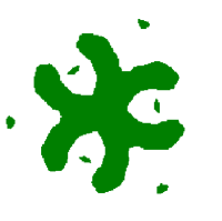
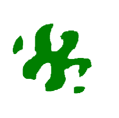
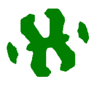
For the best configurations found by the simulations exhibit unexpectedly complex disconnected shapes. In the interval we found three distinct types of shape, which are shown in Fig. 9. Each shape appears optimal for only a small range of within this interval. The simulations also frequently generated suboptimal configurations corresponding to local maxima (such configurations will be discussed in Sec. VI.5).
For the best shape found has three-fold rotational and mirror symmetries (see left panel of Fig. 9), corresponding to the dihedral group . Despite being superior to other types of configuration generated in this range of , the three-fold shape was only infrequently found by the simulations, suggesting that it is located at a maximum that is difficult to reach. The best shape found for appears to lack any symmetry. It is shown in the middle panel of Fig. 9. Close to a transition to a roughly “H”-shaped solution with additional disconnected patches was observed. This shape, shown in the right panel of Fig. 9 is mirror symmetric around two orthogonal axes, corresponding to the dihedral group . Configurations of this type were the best found for . At the generated H-shaped configurations had nearly the same as the asymmetric ones, suggesting that the transition between the asymmetric and the H-shaped regimes occurs close to . H-shaped configurations were also occasionally generated as (apparently) nearly optimal configurations for values of between 0.59 and 0.66, while the asymmetric configurations were frequently generated for between 0.58 and 0.61. As opposed to the three-fold shape, these two types of configuration appear to be located in maxima of the model that are easier to reach. The abundance of different shapes generated in this regime and the rapid transitions between them as is varied suggest that this regime has a particularly interesting and complex landscape. It also makes it more plausible that not all maxima in this regime have been explored in the present setup and better configurations might yet be discovered.
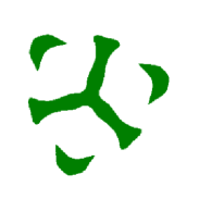
VI.3 Three-bladed fan regime
For the best configurations found are shaped like a three-bladed “fan” with additional patches between the blades, as shown in Fig. 10. These configurations have three-fold rotational and mirror symmetries, corresponding to the dihedral group . Starting from approximately a hole starts to develop in the centre of the fan. The hole becomes larger with increasing . The three-bladed fan was also occasionally generated as an (apparently) nearly optimal configuration at larger values of .


VI.4 Stripes regime
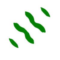
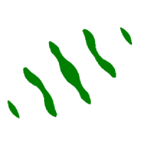
As is further increased, the best configurations found by the simulations comprise four roughly parallel “stripes” of finite length. The transition occurs close to where the values of for the fan and the stripes configurations are comparable. Configurations with five stripes were also sometimes generated, but had lower . The distance between the stripes roughly corresponds to and their boundaries consist of several curved segments. Stripes that are further away from the centre are thinner and shorter than the central ones. The configuration with four stripes appears related to the H-shaped configuration, with the connecting part missing and the disconnected patches further apart. Like the H-shaped configuration, the stripes configurations is mirror symmetric around two orthogonal axes, corresponding to the dihedral group .
For the range considered in this work, no configuration with more than five stripes was found. We do not know whether configurations with more stripes will emerge for larger . Figure 11 shows an example of a four striped configuration found to be the best for and a five striped configuration found to be nearly as good.
VI.5 Summary of numerical results
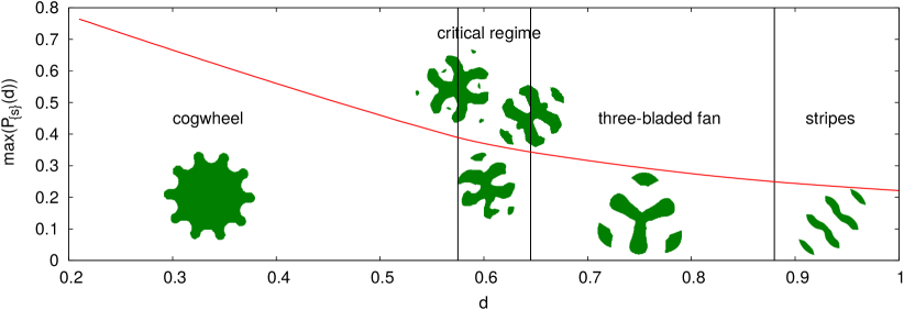
Figure 12 summarises the “phase diagram” of the different regimes with corresponding highest values of obtained in the default setup.


As discussed in the previous sections, the system occasionally annealed to suboptimal configurations, corresponding to local maxima of . Usually these configurations were of a shape type that was the best found for other values of , but sometimes new shapes were also generated. Examples of such shapes are shown in Fig. 13. Of course, it is possible that other near-optimal (or even optimal) shapes exist which were not found by the present simulations. In particular, shapes with very fine structures that cannot be resolved with the present discretization would require larger values of .
VII Discussion and outlook
In summary, we take our numerical results as strongly suggesting a qualitative description of the broad features of solutions to the grasshopper problem for the ranges of investigated. This description remains consistent under various non-trivial consistency checks, and is also consistent with our analytic results. We hope that further refining our discretization may allow a sufficiently precise description of the apparently optimal configurations to allow the possibility of conjectures amenable to analytical proof. It should also allow a more precise characterisation of the values of defining transitions between regimes that characterise qualitatively different shapes, particularly those around the range , where the solution space appears to have a particularly complex structure.
Further numerical and analytic investigations are thus definitely merited. It would also be worthwhile to study the behaviour of the spin model itself in greater detail. The focus of this work is on finding the ground state of the system. Other interesting questions include the behaviour of the system at finite temperatures (and possible associated transitions), as well as transitions associated with varying lattice size and number of spins, thermalization times, the calculation of thermodynamic observables, and so on.
We would not necessarily expect our results for large to extrapolate well to the grasshopper problem on the sphere when the lawn has the area of the hemisphere. Because the sphere is compact, a large jump from what appears to be an outer edge of a lawn, in any direction, could return the grasshopper to the lawn. For small , however, the construction of Lemma suggests that the hemisphere is not optimal, and it seems plausible that cogwheel-type solutions will again emerge. This does not, however, give any definitive insight into the solutions of versions of the problem relevant to Bell inequalities, since these require (at least) the antipodal condition as an additional constraint. The construction of Lemma does not generalise to a construction of an antipodal lawn on the sphere, at least in any straightforward way, and our numerical cogwheel solutions do not generally appear to either. It thus remains plausible that the antipodal condition is significantly relevant and that the hemisphere is optimal for small among antipodal lawns. Now that our numerical techniques are well tested in the planar case, it should be simple to transfer them to the spherical case and thus resolve this question.
There are many other questions related to and generalizations of the grasshopper problem that it would be interesting to address. We list some of these here.
Restrictions on the lawn: Interesting restrictions include requiring that the shapes be connected, or simply connected, or convex. Our results suggest that each of the last three is a genuine restriction.333Note that, if the optimal shape is disconnected, there will exist sequences of connected shapes with success probability tending to the optimal probability. Such shapes can be constructed from the optimal shape by subtracting small areas from the optimal lawn and then connecting all its disconnected parts by suitably thin strips. The optimal shape appears to be non-convex for any value of , and not connected for large .
Variable density lawns: It seems natural to allow lawns of less than unit density, but unclear whether such lawns might actually be optimal for any value of . That is, does there exist a jump distance with an optimal probability density such that the set has measure less than one? Our results to date are consistent with the optimal density always being an identity function: that is, with the density of the optimal lawn always being one or zero.
The spin models, which give numerical evidence about the form of optimal lawn configurations, also effectively assume unit density lawns at their finest scale of resolution. There are alternatives to this discretization scheme. One could, for instance, allow intermediate spin values between 0 and 1. This may not be necessary, since it seems plausible that a simulation of the regular discretized model could effectively produce such a density function without allowing intermediate spin values. For example, a checkerboard lawn region is a simple discretized model of a lawn region with . Alternatively, if the small-scale checkerboard regularities turn out to have a significant effect, a continuum lawn region with could be modelled by a discretized region in which the grid cells are independently randomly and equiprobably filled () or empty (). More generally, a continuum lawn region with density could be modelled by a discretized lawn region in which a proportion of the cells are randomly filled. One might thus hope that the existing discretized model would identify optimal lawns with non-uniform density, if any exist. Our numerical results so far do not suggest any optimal lawns of this type. Finer scale discretizations would allow further investigation of this question.
Generalisations to other dimensions: The problem generalises to for any positive integer . The case is easy to solve. Consider the lawn defined by the segments , , , . This has total length and gives a probability of the grasshopper remaining on the lawn. The sequence of such lawns for positive integer thus gives us the supremum value for the probability. This class of solutions, whose members are periodic over increasingly large ranges and have success probabilities increasingly close to , appears to have no analogy in higher dimensions, where the problem seems much harder. Intuitively, this appears to be because of a mismatch between the dimensionality of the jump and the space in which it takes place.
Generalisations to other spaces: The grasshopper problem also seems interesting and natural on other Riemannian manifolds. One example is the surface of the sphere – and indeed the problem was originally motivated by the case of . The grasshopper problem seems particularly natural on the sphere, as on the plane, since jumps of fixed distance in any direction are related by the sphere’s rotational symmetry. Another interesting example is the torus , obtained by identifying the edges of a hypercube in the usual way. While this has a lower degree of symmetry than the sphere, it lends itself naturally to discretization by lattices with periodic boundary conditions. For both the sphere and torus the solution must in general depend on the ratio of the lawn volume to the manifold volume. So, if we keep the convention that the lawn has volume one then we should consider the manifold volume (or equivalently the sphere radius or the hypercube edge length) as a second variable in the problem along with .
Generalisations to other metrics: Rather than using Euclidean distance (the norm) we can consider a different metric, for instance the Manhattan metric defined by the norm. The latter is particularly interesting for the discrete version of the grasshopper problem on a square grid, which can be studied with a spin model. In this case there is no error in the distance measurement associated with the discretization of the system. Alternative grids, for instance hexagonal, can also be studied with the appropriate definitions of Manhattan distance.
Extensions of the problem: The grasshopper problem can be naturally extended in a number of ways. One variation, which is motivated by our original Bell inequality problem Kent and Pitalúa-García (2014), is to allow two independently defined lawns, using two different species of lawn seed that can coexist in the same region, with each independently allowed any density between zero and one inclusive. In this version of the problem the grasshopper lands randomly on the first lawn and jumps as above. The aim is to find a pair of lawn configurations that maximises the probability that it ends up on the second lawn.
Other variations of the single lawn grasshopper problem allow independent random jumps of distance , either simply requiring that the grasshopper is on the lawn after the -th jump, or else imposing the condition that it must also be on the lawn after each jump. One could also allow a variable random jump distance, for example Poisson distributed with mean .
Another interesting variant is the ant problem, which is defined for lawns of unit density. Like the grasshopper, the flying ant arrives at a random point on the lawn. It then sets out to walk a distance in a random direction. Alas, however, if at any point it leaves the lawn, it dies. It seems clear that disconnected lawn shapes will not be optimal for any in this case. Moreover, it is not evident that the shapes optimal for the grasshopper problem are optimal for the ant problem for any .
A further alternative is to model the grasshopper (or the ant) when external forces influence its trajectory. For example, we can define a simple model of the grasshopper in a breeze by supposing that a fixed vector is added to the random length vector defining its regular jump.444The breeze could be modelled more realistically by modelling an actual jump trajectory with fixed initial angle of elevation and speed, taking into account the breeze force and gravity. Another interesting variation along these lines is to model the grasshopper’s trajectory under gravity (not necessarily with any breeze) when jumping on an inclined plane or other embedded manifold. It would also be interesting to understand the properties of the corresponding spin models, which describe an anisotropic interaction whose range is fixed in any given direction but varies with the direction.
Applications to catalytic reactions: One source of motivation for several of the variations above is that the grasshopper problem defines a simple model of catalytic reactions that give significant impetus to the catalyst. For example, consider a chain reaction in which a randomly selected nucleus of an atom of element is impacted by a high energy particle and undergoes fission. Suppose that the fission process produces a further particle of fixed energy, independent of the energy of the original particle , which travels a distance before becoming near stationary. At this point, if surrounded by atoms of the same type , it will be absorbed by another nucleus, again causing fission, and so on. Suppose that there are a finite number of atoms of type contained in a region . Suppose also that the region is surrounded by atoms of element that slow the particles at the same rate as those of element , so that the particles travel the same distance whether they remain in or not. However, if they come to rest surrounded by type atoms, they undergo no further reactions. A reaction of this type can be modelled by the grasshopper problem in the relevant number of dimensions (three if the region is unconstrained, two if it is constrained to be a thin solid, with fixed height and constant cross-section). The maximum initial reaction rate arises when the region solves the grasshopper problem.
Applications to morphogenesis: Our numerical solutions strikingly illustrate the emergence of structures with discrete symmetries from an isotropic problem with continuous rotational symmetry. They also bear at least a passing resemblance to patterns seen elsewhere in nature, including the contours of flowers, the patterns seen on some seashells and the stripes on some animals.
Turing’s well-known theory of morphogenesis Turing (1952) hypothesises that many such natural patterns arise as solutions to reaction-diffusion equations. This possibility has been demonstrated experimentally Tompkins et al. (2014). Our results suggest that a rich variety of pattern formation can also arise in systems with effectively fixed-range interactions, including interactions associated with the sort of catalytic reaction described above. It may be worth looking for explanations of this type in any context where highly regular patterns naturally arise and are not otherwise easily explained.
Further applications to quantum information theory: Our investigation was motivated by analysing specific Bell inequalities that distinguish the predictions of quantum theory for a two qubit singlet state from those of local hidden variable theories. These particular inequalities have an especially simple geometric interpretation which generalises to the plane and other surfaces.
Spin models amenable to simulated annealing and parallel tempering could also be used to investigate other types of Bell inequality for pairs of qubits and higher dimensional entangled states. It would be very interesting, for example, to apply them to the problem of finding the full ranges of Werner states Hirsch et al. (2017) that can be simulated by local hidden variable models, and to explore similar questions for other interesting entangled states, including multipartite states.
Nor are our techniques restricted to analysing Bell inequalities. A local hidden variable model is effectively a classical algorithm for simulating quantum theory, and our motivating goal is to find the best such classical algorithm according to a natural metric. Simulated annealing and parallel tempering methods can also be applied to search for more general classical algorithms that optimize a quantity of interest. In particular, they could be applied to other problems of interest in quantum information theory, including problems of quantum communication complexity. One relatively simple example is the problem of finding algorithms that simulate quantum correlations with shared randomness and finite one-way classical communication Toner and Bacon (2003). For projective measurements on pairs of qubits, such algorithms can be thought of as generalised grasshopper models, in which Alice has a single lawn, Bob has a set of available lawns, and Alice chooses which of Bob’s lawns is used in each given run.
Acknowledgements
We are grateful to Chris Amey, Simon Lentner, Jonathan Machta and Mykhaylo Tyomkyn for interesting and helpful discussions. This work was supported by an FQXi grant and by Perimeter Institute for Theoretical Physics. Research at Perimeter Institute is supported by the Government of Canada through Industry Canada and by the Province of Ontario through the Ministry of Research and Innovation. OG is funded by the NSF under the Grant No. PHY-1314735.
References
References
- Bell [1964] John Stuart Bell. On the Einstein-Podolsky-Rosen paradox. Physics, 1:195–200, 1964. Reprinted in John Stuart Bell, Speakable and Unspeakable in Quantum Mechanics, Cambridge University Press, 1987.
- Clauser et al. [1969] John F Clauser, Michael A Horne, Abner Shimony, and Richard A Holt. Proposed experiment to test local hidden-variable theories. Phys. Rev. Lett., 23(15):880–884, 1969. doi: 10.1103/PhysRevLett.23.880.
- Kent and Pitalúa-García [2014] Adrian Kent and Damián Pitalúa-García. Bloch-sphere colorings and Bell inequalities. Phys. Rev. A, 90(6):062124, 2014. doi: 10.1103/PhysRevA.90.062124.
- Littlewood and Bollobás [1986] John Edensor Littlewood and Béla Bollobás. Littlewood’s miscellany. Cambridge University Press, 1986.
- [5] Euclid. Elements.
- Croft et al. [1991] Hallard Croft, Kenneth Falconer, and Richard Guy. Unsolved problems in geometry. Springer, 1991.
- Bukh [2008] Boris Bukh. Measurable sets with excluded distances. Geometric and Functional Analysis, 18(3):668–697, 2008.
- [8] S. Lentner. Private communication.
- Peskin [2002] C. S. Peskin. The immersed boundary method. Acta Numerica, 11:479–517, 2002. doi: 10.1017/S0962492902000077.
- Yang et al. [2009] Xiaolei Yang, Xing Zhang, Zhilin Li, and Guo-Wei He. A smoothing technique for discrete delta functions with application to immersed boundary method in moving boundary simulations. J. Comput. Phys., 228(20):7821–7836, 2009. doi: 10.1016/j.jcp.2009.07.023.
- Newman and Barkema [1999] M. E. J. Newman and G. T. Barkema. Monte Carlo Methods in Statistical Physics. Oxford University Press, 1999.
- Kirkpatrick et al. [1983] S. Kirkpatrick, C. D. Gelatt, and M. P. Vecchi. Optimization by simulated annealing. Science, 220:671–680, 1983. doi: 10.1126/science.220.4598.671.
- Hukushima and Nemoto [1996] K. Hukushima and K. Nemoto. Exchange Monte Carlo Method and Application to Spin Glass Simulations. Journal of the Physical Society of Japan, 65:1604, June 1996. doi: 10.1143/JPSJ.65.1604.
- Turing [1952] Alan Mathison Turing. The chemical basis of morphogenesis. Bulletin of Mathematical Biology, 52(1):153–197, 1952.
- Tompkins et al. [2014] Nathan Tompkins, Ning Li, Camille Girabawe, Michael Heymann, G Bard Ermentrout, Irving R Epstein, and Seth Fraden. Testing Turing’s theory of morphogenesis in chemical cells. Proceedings of the National Academy of Sciences, 111(12):4397–4402, 2014. doi: 10.1073/pnas.1322005111.
- Hirsch et al. [2017] Flavien Hirsch, Marco Túlio Quintino, Tamás Vértesi, Miguel Navascués, and Nicolas Brunner. Better local hidden variable models for two-qubit Werner states and an upper bound on the Grothendieck constant . Quantum, 1:3, April 2017. ISSN 2521-327X. doi: 10.22331/q-2017-04-25-3.
- Toner and Bacon [2003] B. F. Toner and D. Bacon. Communication cost of simulating Bell correlations. Phys. Rev. Lett., 91:187904, Oct 2003. doi: 10.1103/PhysRevLett.91.187904.